
Discrete-Time Pole-Region Robust Controller for Magnetic Levitation Plant


Institute of Automotive Mechatronics, Slovak University of Technology in Bratislava, UAMT FEI, 812 19 Bratislava, Slovakia
*
Authors to whom correspondence should be addressed.
†
Current address: FEI STU, Ilkovičova 3, 812 19 Bratislava, Slovakia.
‡
These authors contributed equally to this work.
Symmetry 2021, 13(1), 142; https://0-doi-org.brum.beds.ac.uk/10.3390/sym13010142
Submission received: 7 December 2020
/
Revised: 11 January 2021
/
Accepted: 13 January 2021
/
Published: 16 January 2021
(This article belongs to the Special Issue PID Control and Symmetry)
Abstract
:Robust pole-placement based on convex -regions belongs to the efficient control design techniques for real systems, providing computationally tractable pole-placement design algorithms. The problem arises in the discrete-time domain when the relative damping is prescribed since the corresponding discrete-time domain is non-convex, having a “cardioid” shape. In this paper, we further develop our recent results on the inner convex approximations of the cardioid, present systematical analysis of its design parameters and their influence on the corresponding closed loop performance (measured by standard integral of absolute error (IAE) and Total Variance criteria). The application of a robust controller designed with the proposed convex approximation of the discrete-time pole region is illustrated and evaluated on a real laboratory magnetic levitation plant.
1. Introduction
Robust control belongs to widely used control strategies implemented in real applications, since the real world plants always include uncertainties due to modeling errors, nonlinearities and other influences. Real plants are mostly nonlinear; however, to simplify the analysis and control, often the linearized model is used together with robust, adaptive or other control design techniques appropriate for uncertain linear systems; an excellent survey of various robust control approaches can be found in [1]. The important type of uncertain system model is a polytopic one, which can be advantageously used to formulate the robust control problem in the computationally tractable Linear Matrix Inequality (LMI) form [2]; related recent results based on the so-called S-variable approach are presented in [3]. Besides stability for all uncertain parameter values, a closed loop performance is an important factor in successful robust control design. Various approaches exist to consider performance both in state space and frequency domains; pole-placement belongs to efficient techniques for achieving the prescribed closed-loop dynamics, [4,5,6,7,8] and others.
In real plant control design, it is often desirable to place the closed-loop poles into the prescribed region of the complex plane instead of prescribing their exact position, for example, to achieve the determined stability degree or relative damping. The pole region approach is also appropriate for robust control of uncertain systems, where the exact pole placement is impossible. Significant results have been obtained in this field during the past two decades when the so-called LMI, or more generally, the region approaches have been established and used for robust control design in state space [3,4,9]. When used in robust control, regions are formulated as convex domains in the complex plane, symmetric about the real axis, corresponding to the specific subset of the stable domain defined to achieve the determined performance (closed-loop dynamics). The LMI formulation of generalized stability condition enables efficient computation of the corresponding feedback controller gains [2,3,4,10]. There is a tight connection between closed-loop poles and other performance indices, such as settling time and stability margin [5,6,7]. A major part of the published results on LMI based pole-placement; however, considers the continuous-time case, where standard pole regions for prescribed stability degree and relative damping are convex and can be directly applied to the developed robust state feedback control design schemes, [3,7,8,11]. For the discrete-time systems, however, the pole region for the prescribed relative damping is no longer convex, which causes a specific problem and can be sensed as a kind of asymmetry with the continuous-time counterpart. To simplify the controller design, some variants of a convex approximation of the non-convex cardioid pole-region have been presented [12,13,14,15,16]. In [12], an inner circle is proposed, which in [15] is enlarged to an inner ellipse. These approximations are relatively simple, however, they do not include the neighborhood of point [1, 0], which can cause problems in some real system applications, as will be demonstrated in this paper. Other inner approximations of the non-convex discrete-time pole region are developed in [13,16]. In [13], a cross-section of two cones is proposed, and in our recent paper [16], several inner approximation possibilities are presented together with the corresponding matrices defining the respective region. In this paper, the above results on discrete-time pole-regions are further developed and thoroughly studied on the laboratory magnetic levitation plant.
Magnetic levitation belongs to challenging plants to control, due to its nonlinearity, instability and fast dynamics, with broad application area. Many authors devoted their research to modeling and control of a magnetic levitation system, [17,18,19,20,21,22,23,24]. In [17,21], a linearized model of magnetic levitation is derived based on first principles, the former uses Jacobian linearization, while the latter applies a general linearization technique. Various continuous-time control schemes for magnetic levitation can be found, for example, feedback linearization approach in [18], CDM based design in [19], adaptive state feedback [20]; in all these papers, the results were verified by simulation. To the authors’ best knowledge, there are no papers on discrete-time pole-placement for magnetic levitation, besides our recent results [16,23,24]. In [23,24], we designed a discrete-time pole-placement controller for prescribed relative damping using inner approximation of the non-convex pole domain by an ellipse in the former and by angle-ellipse domain in the latter case. In [16], the computations of the matrices defining the regions appropriate for discrete-time pole-placement are presented.
In this paper we further extend our previous results. A comprehensive study of discrete-time robust controller design for magnetic levitation laboratory plant is presented. The main contribution is a thorough systematic analysis of design parameters, their influence on achieved closed-loop pole position and closed-loop performance measured by standard performance criteria: integral of absolute error (IAE) and Total Variances for input and output variables. In addition, the relationship between pole-placement design parameters and the above performance criteria is studied. The proposed discrete-time pole-placement approach is systematically evaluated for changing design parameters on a real laboratory plant. Comparison of the received results with standard robust controller design using a D-partition method is provided as well. The results obtained from the real plant show the efficiency of the presented discrete-time pole-placement robust controller design.
2. Preliminaries and Problem Formulation
As a model of a controlled system, we will consider an uncertain dynamic system described in state space by its linearized discrete-time model
where is the state vector, is the control input, denotes the vector of uncertainty parameters corresponding to polytopic uncertainties. Polytopic uncertainties of state model matrices are described as
where are constant matrices of corresponding dimensions. We assume that all state variables are at disposal for a state feedback control
The resulting closed-loop system is then given by
The aim of a controller design is to modify the dynamics of the controlled uncertain system (1), (2) so that the corresponding closed-loop system (CLS) (4) is stable and meets the prescribed performance requirements.
Various performance specifications can be used to determine appropriate CLS (4) behavior. The CLS dynamics is basically determined by the CLS poles. Basic performance measures, such as overshoot, settling time, relative damping, decay rate, strongly depends on CLS poles. When an uncertain system is considered, the system model belongs to the whole set of system models and the poles cannot be placed into certain points for the whole uncertainty domain, therefore in this case the required pole region is defined where the CLS poles should lie. The convex region approaches for pole placement using LMI or ones, have been developed in past decades to simplify the computation load, [4,9]. The basic definition of a general region is in the next subsection.
2.1. Regions
A region of the complex plain is defined, [9], as
With the assumption that is positive definite (semidefinite), the region is convex and can be equivalently described by LMI. Matrix is said to be stable if and only if all its eigenvalues lie in the region defined by (5).
Lemma 1
([9]). Closed-loop matrix is stable if and only if there exists a positive definite matrix such that
Remark 1.
It should be noted that (6) can be for an uncertain polytopic system (1), (2) with a state feedback control (3) reformulated as a linear matrix inequality and then solved by some LMI solver, [2,3,4,9] and others. Since solving LMIs is a numerically tractable problem, using regions provide a computationally attractive approach for robust control design.
Standard domains for stable poles and matrices defining the corresponding regions (5) can be listed as:
- Open left-half plane of the complex plane, (continuous-time systems),
- Interior of the unit circle, (discrete-time systems),
- Shifted left-half plane of the complex plane corresponding to stability degree ,(continuous-time systems),
- Interior of the circle centered in [0,0] with radius corresponding to stability degree , (discrete-time systems),
- Interior of the convex cone with vertex angle , corresponding to the relative damping (given by a ratio of the imaginary and real part of the complex pole in continuous-time systems)
Below, for better readability, we use for angle denotation .
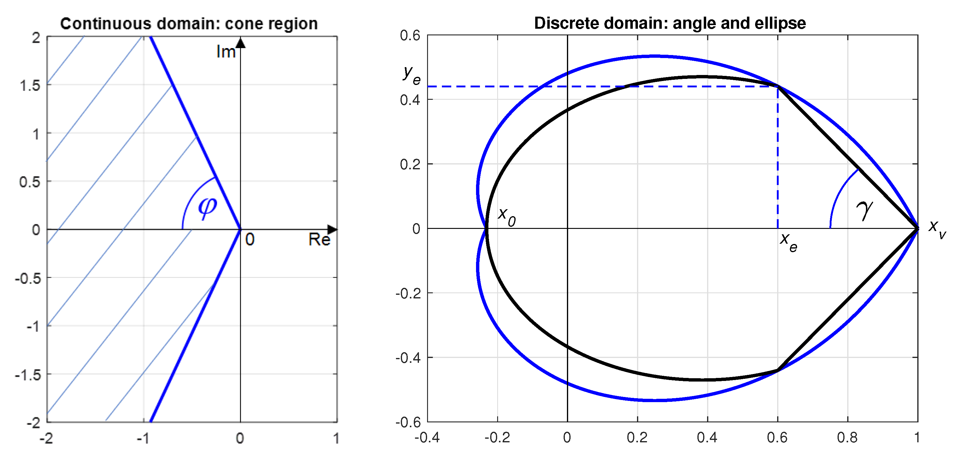
Though the relative damping belongs to basic closed-loop (CL) performance requirements, in this case, the corresponding discrete-time region is no longer convex, and has a cardioid shape as depicted in Figure 1. Recently, we developed a new convex inner approximation of the non-convex cardioid domain [16]. This approximation is referred to as angle-ellipse (AE) and is defined as an intersection of the cone end ellipse, see the right hand part of Figure 1. The cone is defined by its vertex [1, 0] and the intersection point with cardioid ; the ellipse is centered in the middle of the cardioid x-axis, with the y-semi-axis derived so that the ellipse intersects the cardioid in . The corresponding region matrices for AE inner approximation are
where Z is zero matrix; matrices correspond to the ellipse centred in with semiaxes given as
matrices correspond to the cone (shifted angle) given as
2.2. Performance Evaluation
To assess closed loop step responses, the appropriate performance measures are inevitable to quantify the CL system qualities. An important place among standard, frequently used performance measures belongs to Integrated Absolute Error (IAE), [26].
The shapes of transient responses can be quantified concerning deviations from their ideal shapes—a piece-wise monotonicity—in terms of a modified total variation TV (see e.g., [27]). TV performance measures can be applied to evaluate both the input (control) and output variables. Total Variance (TV) can be defined as
Consider now the setpoint step response, and two monotonic intervals as a corresponding ideal input (control) variable shape, with representing an extreme control value, which separates two nearly monotonic input intervals and . Then the control variable performance can be evaluated by a deviation of real control input from two monotonic intervals and quantified by
In Section 4, IAE together with TV performance indices are used to evaluate and compare several designed robust pole-placement controllers. These performance measures will also serve to analyze the control design parameter influences on the closed-loop performance.
3. Magnetic Levitation Plant
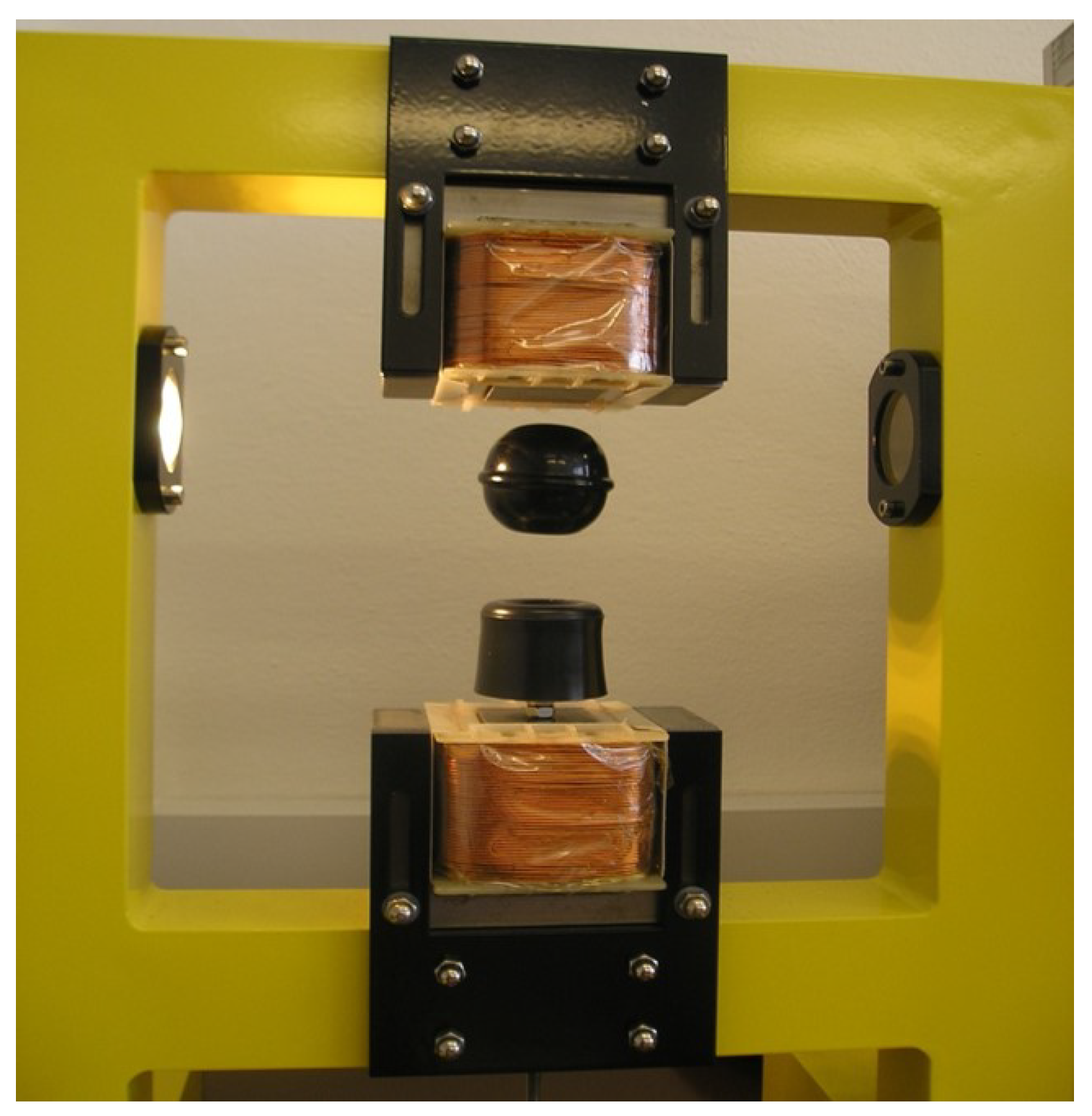
The magnetic levitation laboratory plant (ML), Figure 2, serves as a challenging physical model, which is unstable and has rather fast dynamics [28]. The control aim is to position the levitating ferromagnetic ball within the air-space between two electromagnets. In this paper, we consider the upper electromagnet as an actuator, which compensates the ball (sphere) gravity and determines the ball vertical position.
The nonlinear mathematical model of the laboratory ML can be formulated in state space using three state variables: —position of the ball, —velocity of the ball, —current in the upper electromagnet coil. ML input is the voltage on the upper coil, output is the position of the ball measured from the upper coil.
The corresponding nonlinear model below can be derived using a Lagrange function, see [21]; we omit argument t to improve readability.
where
values for are inherent plant parameters, m is a ball mass, g is acceleration of gravity. All ML parameters are summarized in Table 1.
The ML plant has a discrete-time embedded controller, therefore the robust pole-placement controller is designed from the discretized plant model. The nonlinear continuous-time model (13) can be linearized around the determined working points and then discretized with appropriate sampling period s. The resulting discretized model is described by (1), where matrices have the following form
Elements vary with position of the ball, in Table 2. In the next Section, the following three working points, denoted as WP1, WP2, WP3, and the corresponding discrete-time linearized models are considered for robust pole-placement controller design as the polytope vertices in system model (1) and (2).
4. Robust Controller Design for Magnetic Levitation
In this section we further develop our recent results on discrete-time robust pole-placement controller design, evaluate the design parameters of the proposed approach and compare the results with several other robust controllers. We also analyze the relationship between closed-loop pole position and closed-loop performance measured by IAE and TV defined in Section 2.2.
The robust pole-placement controller is designed for the magnetic levitation described in Section 3, considering linearized uncertain models (1) and (2) for the polytopic domain defined by three working points, as shown in Table 2. The results for the prescribed damping and stability degree based on the inner convex AE approximation of the non-convex domain introduced in Section 2.1 are presented and compared with other results from the literature. The main results can be summarized as follows.
- The influence of AE domain design parameters: , , and r (defining the stability degree), is systematically analyzed and evaluated on a real laboratory magnetic levitation plant. For each parameter, we design several controllers, measure their step responses for three working points (Table 2) and assess their closed-loop performance using performance measures IAE, TV0 a TV1 (described in Section 2.2), the corresponding analysis of design parameters influence on CL performance is presented. Based on the above performance measures, the best controller is chosen.
- Superior controllers received for the AE region are then compared with robust controllers received by alternative approaches: simple robust stability controller placing the poles into a unit circle (UC), [29]; ellipse approximation for the prescribed damping , [23] and with robust continuous-time controllers based on the D-partition approach, [22]; three representative controllers with the smallest overshoot were chosen from the latter approach.
- The last subsection is devoted to analysis of the closed-loop pole position. The prescribed poles are confronted with the obtained closed-loop poles for linearized system; to enable comparison with the continuous-time controller (based on D-partition method), the continuous-time closed-loop poles are recalculated to the corresponding discrete-time ones.
It should be noted that the Magnetic Levitation Plant is a challenging unstable system with fast dynamics. Its dynamics inherently include fast parts corresponding to electrical processes and relatively slower parts corresponding to the ball movement. It is important to consider these characteristics and great care must be taken in determining a realistic required closed-loop pole region. The neighborhood of the stability border, in the discrete-time domain namely vicinity of point [1, 0], must be included otherwise the control variable can trespass feasible intervals; more details are in Section 4.2.1.
4.1. Discrete-Time Robust Pole-Placement State Feedback Controller Design Based on LMI Solution
Robust pole-placement controller for the uncertain polytopic systems (1) and (2) and the region defined by (5) can be directly computed from the LMI corresponding to the respective stability condition (6); see for example, [23]. A corresponding state feedback matrix defining the control law (3) is obtained by a solution to the following LMI
where
are positive definite matrices and , are any matrices. If is zero matrix, to keep the positive definiteness of matrix we consider , where is a small positive number. The resulting state feedback controller matrix is then
The above state feedback controller design scheme can be directly used also for a PI controller design, the state space plant model is then augmented by the PI controller dynamics. The augmented system is then in the form:
where matrix C corresponds to the outputs that should be integrated. The resulting state feedback gain matrix K is then structured as follows
matrices and corresponds to proportional and integral gain of the PI controller. More details can be found in [23].
The main aim of the integration part is to eliminate steady state control error. In magnetic levitation, the ball position should follow the reference value, therefore the state enters the integration term and .
4.2. Discrete-Time Robust Pole-Placement Controller Design Using AE Approximation
In this section we design the state feedback robust controller by solving LMI (15) and (17) for the AE region defined by matrices (7)–(9), adding the stability degree requirement. We systematically changed the AE design parameters:
The evaluation of the corresponding closed-loop performance of the real plant for changing design parameters is presented and the respective step responses are compared.
4.2.1. Design Results for Damping Angle Parameter Changes
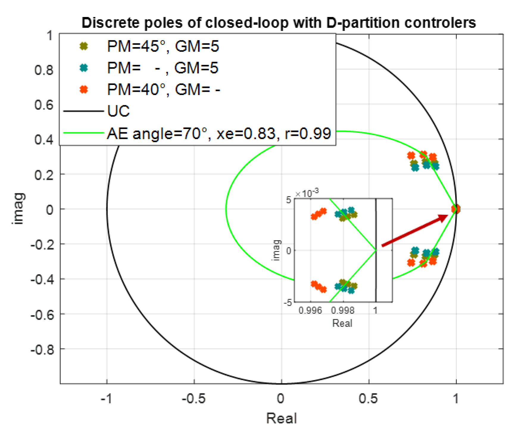
The first studied parameter was , defining the relative damping. Parameters and r were chosen considering the closed-loop pole position from our recent results on robust controller design for magnetic levitation: D-partition based design (continuous-time case) [22] and initial controller from ML system documentation [28]. The closed-loop poles for existing controllers implemented also for a real plant are in the neighborhood of stability border—point [1, 0]. Their maximum modulus is about 0.9985, is above , see Figure 3, however, the closed-loop performance is too oscillating, which is caused by insufficient damping. Our design aim was to improve performance by improving the stability degree and damping to reduce the oscillations. Since the realizable control variable has limited value and the experiments provided sensitivity of the original plant to performance demands that were too strong, we shifted the stability degree and damping only slightly.
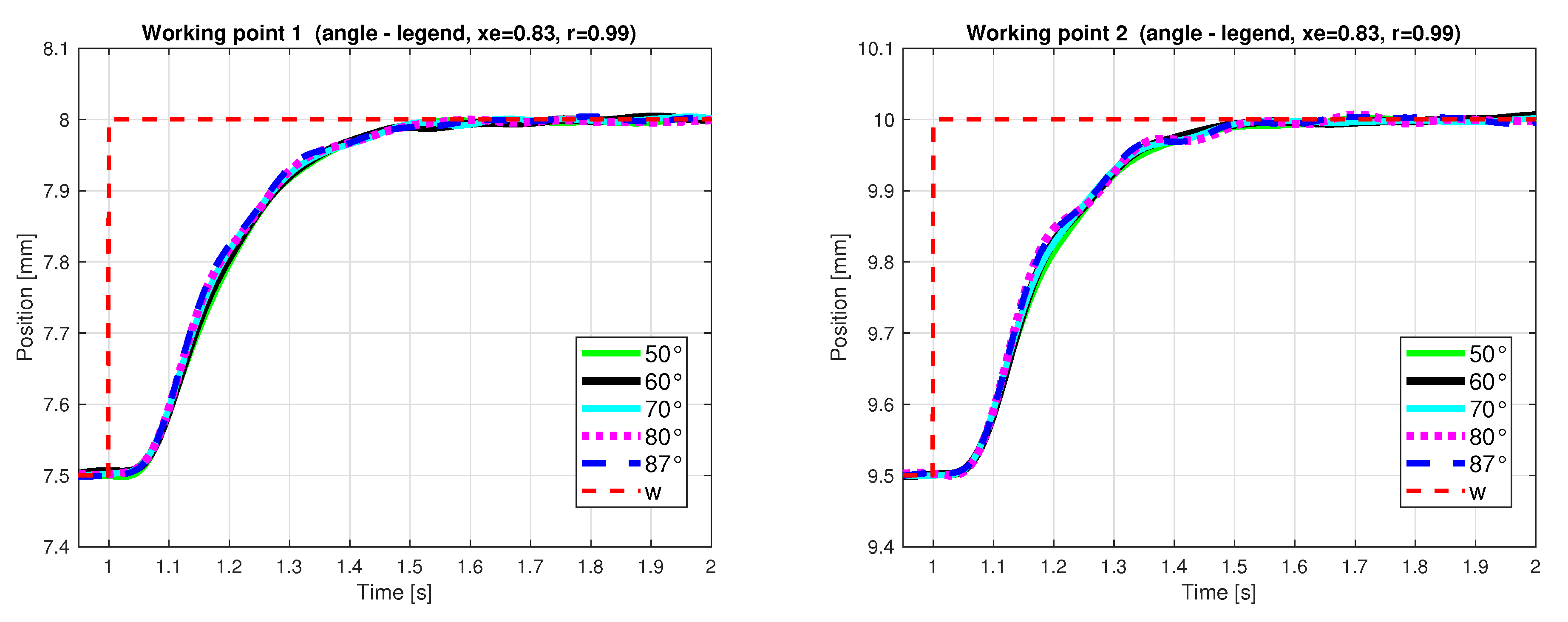
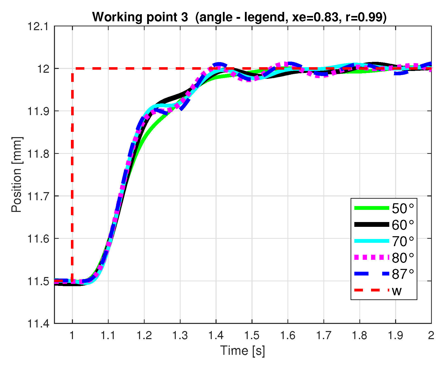
Based on this experience, values and were chosen. In Figure 4 and Figure 5, comparison of real plant step responses is shown for different angles for three considered working points. The closed-loop performance was evaluated for all three WPs, and the results are summarized in Table 3. We also included the mean values and standard deviations of performance measures for all three WP for each parameter configuration, denoted by mean(WP) and stdev(WP), respectively. The best (lowest) values of individual performance measures are marked in green, the best values of mean(WP) are marked in yellow. Standard deviations indicate that the differences between mean values for different angles are statistically significant. Based on the obtained results—step responses and performance measures, the best controllers were chosen for and . Performance criterion TV for output variable clearly indicates that higher damping (lower ) evidently improves output variable step response monotonicity (the damping is physically limited, therefore the best value of yTV0 was received for ).
4.2.2. Design Results for Intersection Parameter Changes
This subsection studies the influence of changing parameter for the fixed values of other design parameters: and .
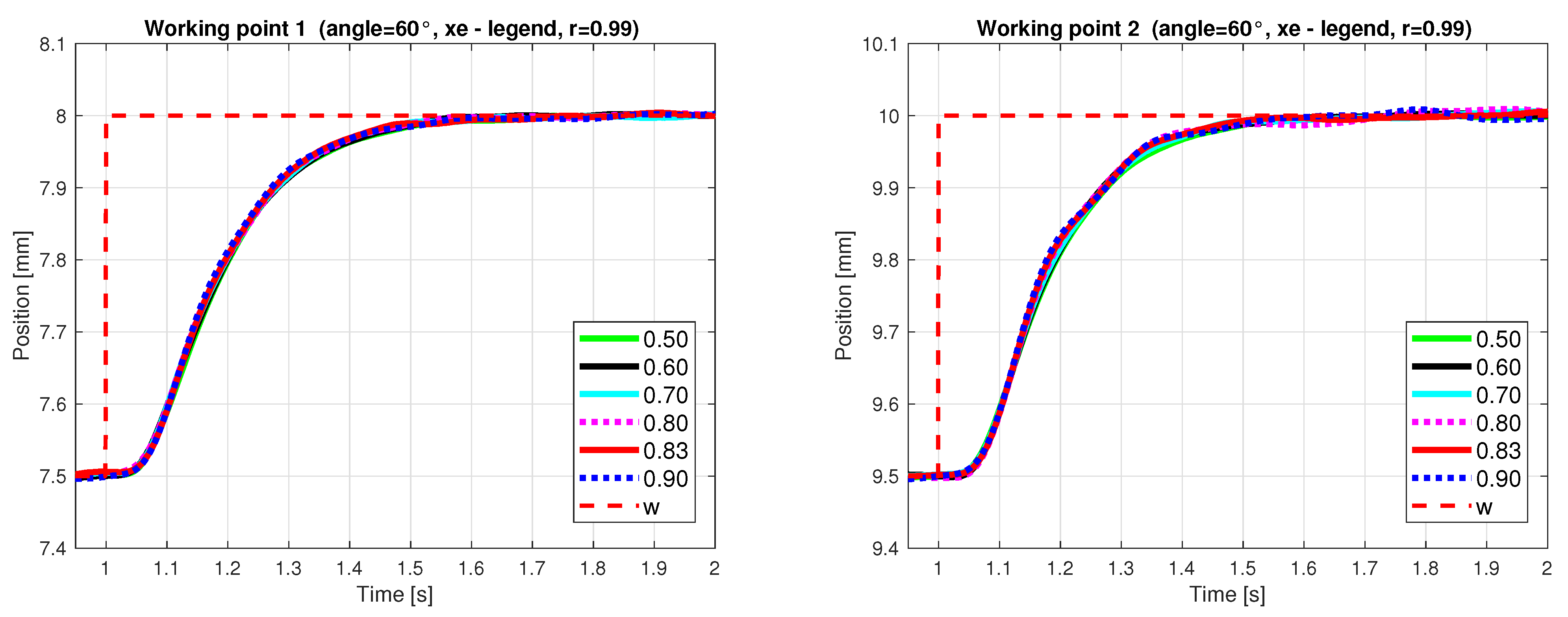
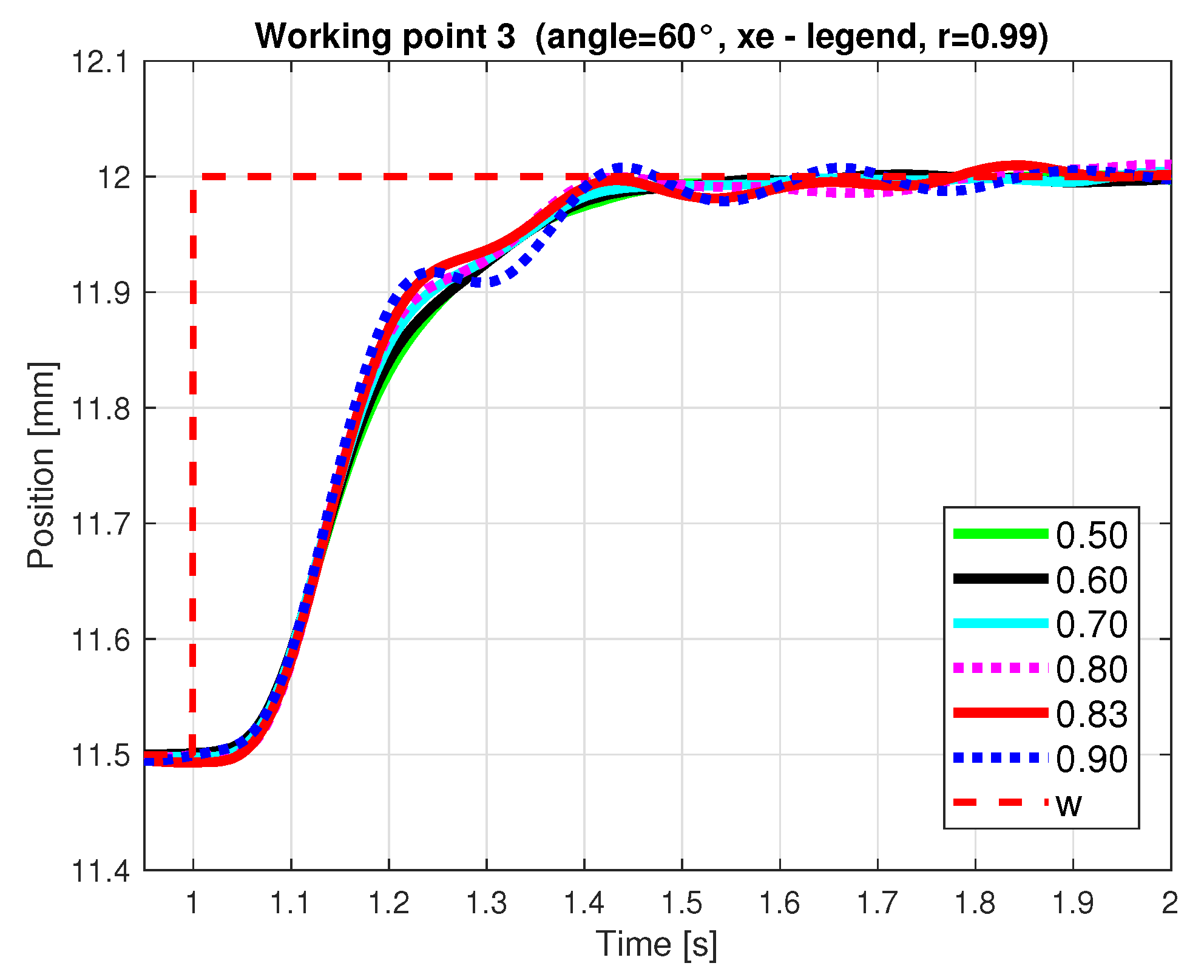
Figure 6 and Figure 7 show step responses of the real plant for the considered three working points. Analogically to the previous subsection, the closed-loop performance was evaluated for all three WPs, and the results are summarized in Table 4. We also included the mean values and standard deviations of performance measures for all three WP for each parameter configuration, denoted by mean(WP) and stdev(WP), respectively. The best (lowest) values of individual performance measures are marked in green, the best values of mean(WP) are marked in yellow. Based on the obtained results—step responses and performance measures for 3 WP, the best controllers were chosen for and . Note that the relatively small standard deviations indicate that there are statistically significant differences between mean values for the considered . The corresponding real plant responses in Figure 6 and Figure 7 confirm superiority of the chosen controller.
4.2.3. Design Results for Changing Stability Degree Radius r
This subsection studies possibilities and influences of changing parameter r for the fixed values of other design parameters: and .
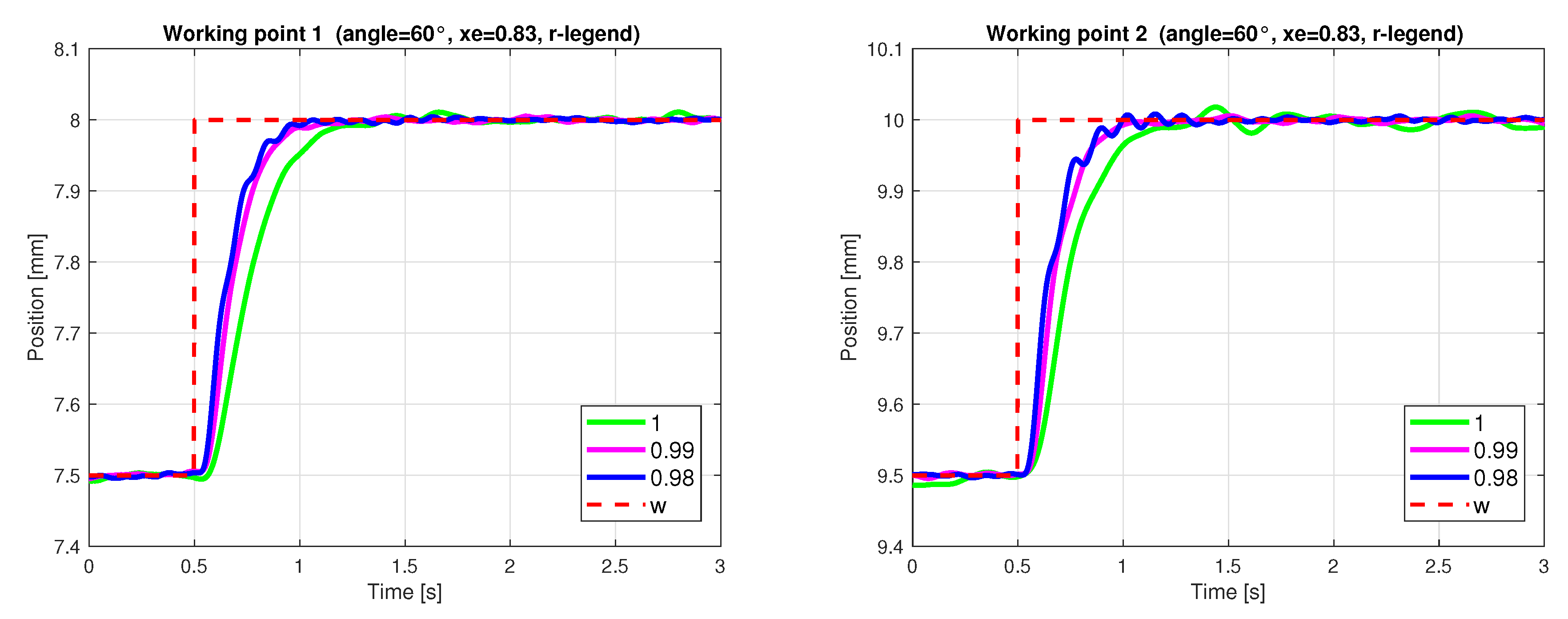
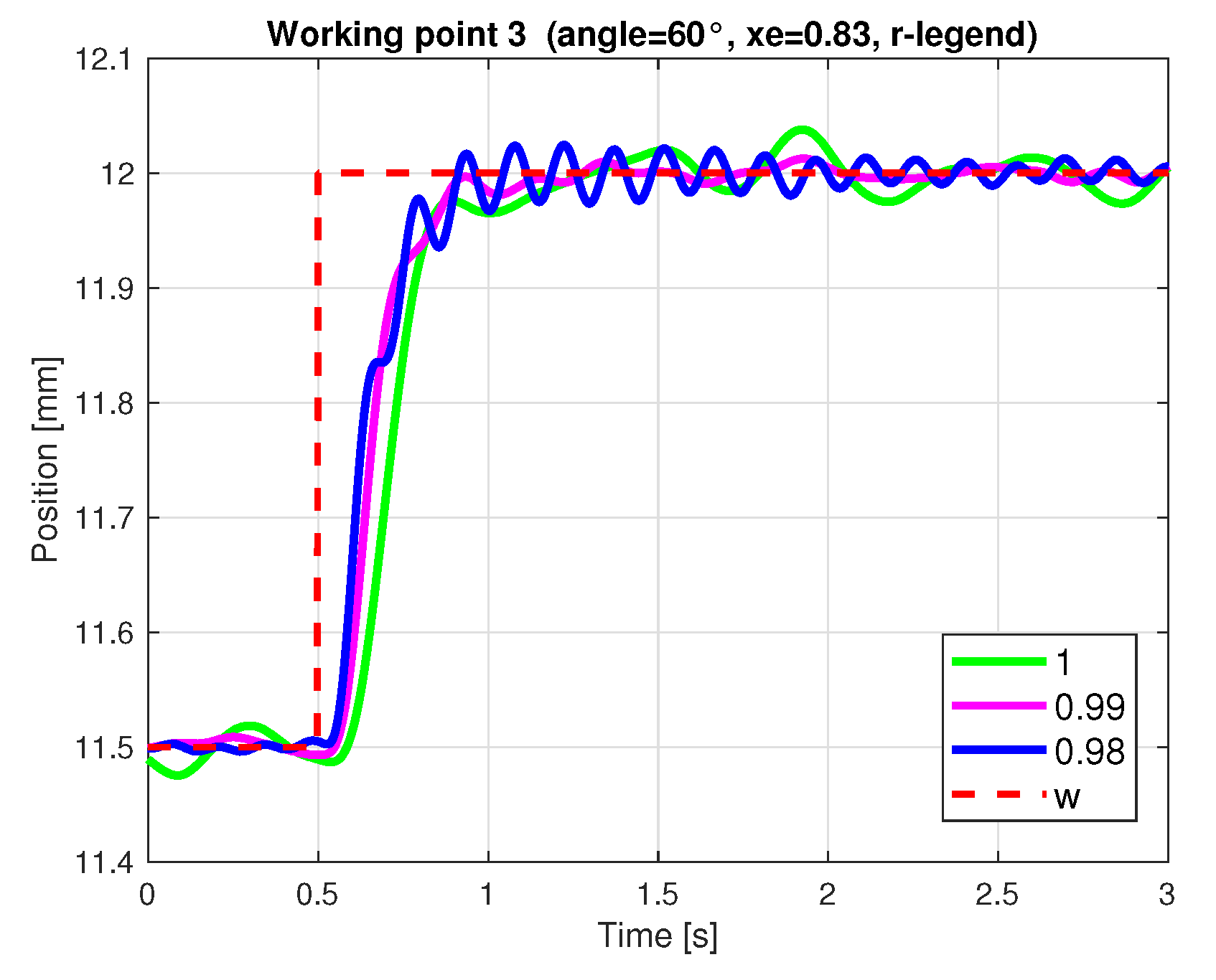
Figure 8 and Figure 9 show step responses of real plants for the considered three working points for varying r. Analogically to the previous subsection, the closed-loop performance was evaluated for all three WPs, the results are summarized in Table 5, and the mean values and standard deviations of performance measures for all three WP for each parameter configuration are denoted by mean(WP) and stdev(WP), respectively. The best (lowest) values of individual performance measures are marked in green, the best values of mean(WP) are marked in yellow. Based on the obtained results—step responses and performance measures for 3 WP, the best controllers were chosen for . Note that the relatively small standard deviations indicate that there are statistically significant differences between mean values for the considered r. The results show that the ML system is very sensitive to the stability degree. Slightly decreased r leads to oscillations since the physical limit of the plant (control variable) is hit. This quality indicates that to improve performance, it is important to engage other design parameters. AE approximation provides relative damping defined by and also the intersection limiting the imaginary parts of the CL poles in the neighborhood of point [1, 0].
4.3. Comparison of Robust Controllers: AE with Other Convex Approximations and Continuous-Time Controllers
In this section, we compare the best robust discrete-time pole-placement controllers designed in the previous subsection using the AE region, with robust controllers designed for magnetic levitation by other approaches
- Stabilizing controllers (closed-loop poles in unit circle), [29]
- Pole-placement controllers for the prescribed relative damping, based on ellipse inner approximation of the non-convex cardioid domain, [23]
- Continuous-time robust controllers based on D-partition, [22].
Parameters of all considered discrete- and continuous-time controllers are listed in Table 6 and Table 7.
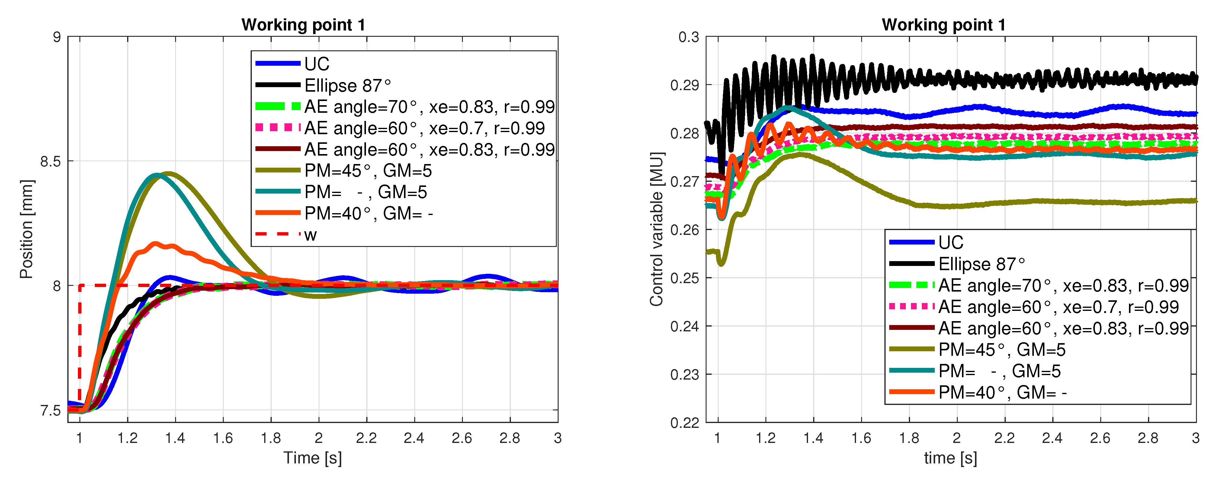
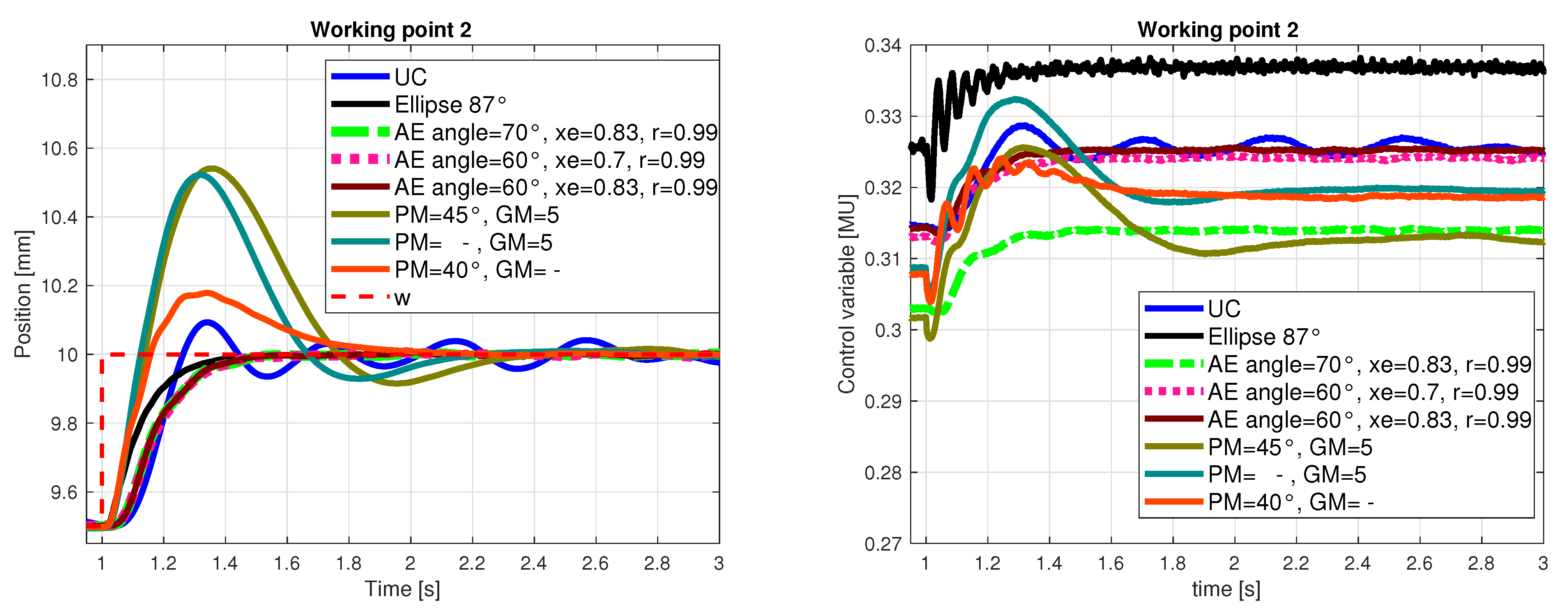
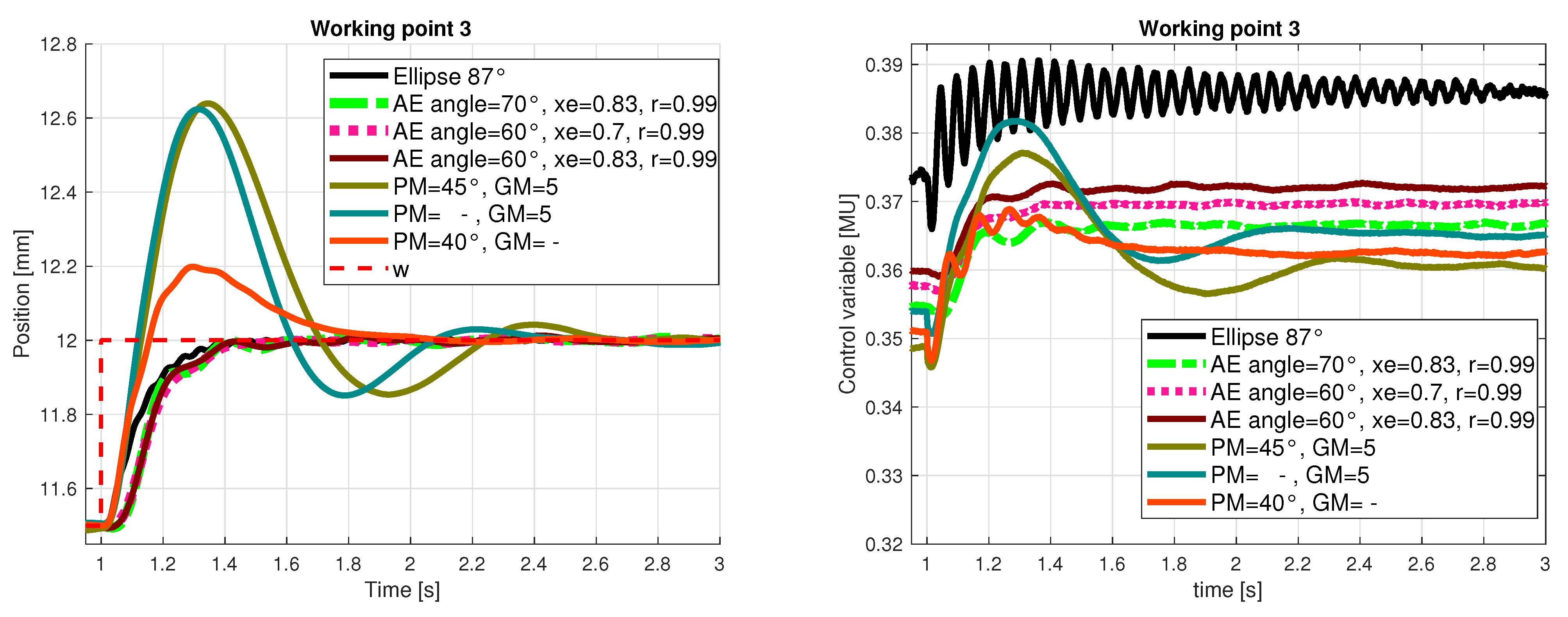
The corresponding real plant step responses in all three WP are shown in Figure 10, Figure 11 and Figure 12 both for output and control variables. Overall performance evaluation is summarized in Table 8. The performance evaluation is calculated for individual WP and the mean value for all three WP (mean(WP)) is included in the fourth row for each designed controller. The best performance for individual WP is marked in green, the best value of mean(WP) is marked in yellow.
The obtained results illustrate the performance superiority of the proposed AE based controllers.
4.4. Closed-Loop Pole Analysis
This section analyzes and compares the closed-loop pole position for the controllers presented in Section 4.3. In all cases, the closed-loop poles (CLP) are shown for all three considered working points.
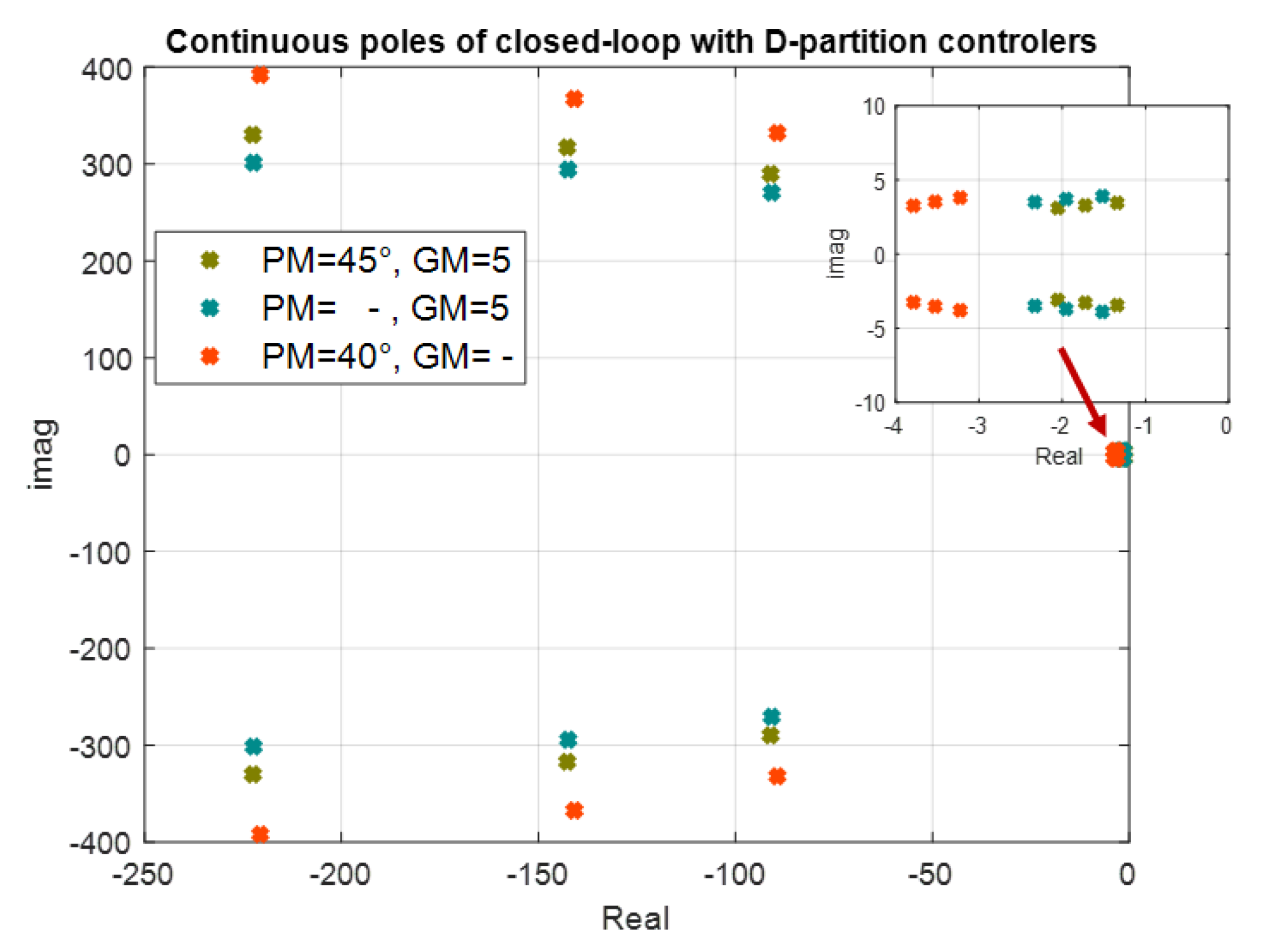
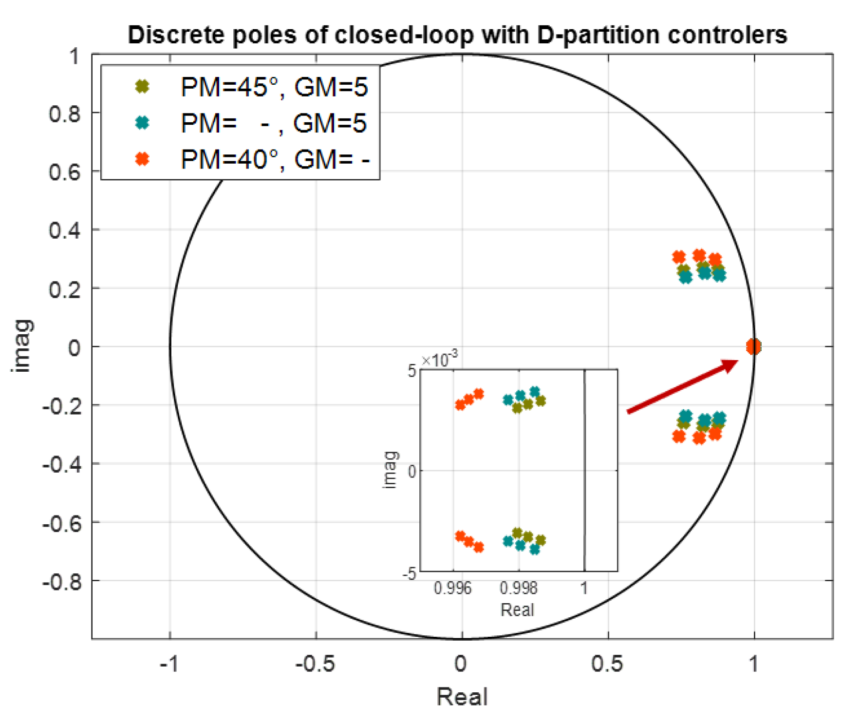
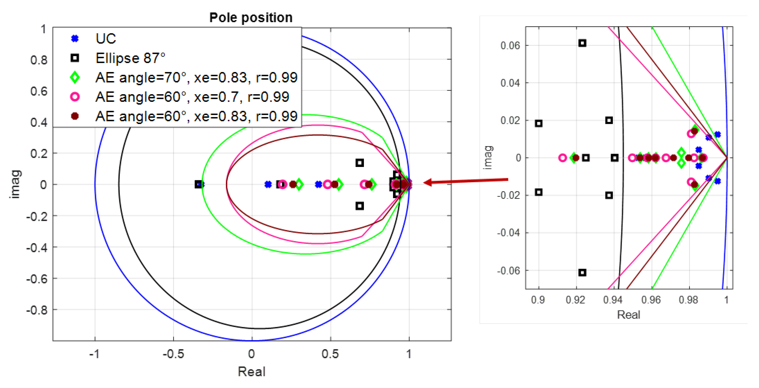
We start with the CLP for the continuous-time robust controller. In Figure 13, CLP are depicted corresponding to controllers designed by the D-partition with various phase and gain margins, [22]. We transformed the CLP for the continuous-time system into a discrete-time domain for the above defined sampling time s, these recalculated discrete-time CLP are shown in Figure 14. The neighborhood of boundary point [1, 0] is shown in detail, notice that there are poles rather close to stability boundary. Figure 15 displays CLP obtained for the discrete-time robust controllers, the pole regions considered in design are depicted as well. Again, the neighborhood of [1, 0] is shown in detail. It can be seen that the obtained CLP are inside the prescribed domains, therefore in Table 9 we summarize the achieved stability degree and —the angle of the discrete-time region (see the right hand side picture in Figure 1). For comparison, in Table 10 we summarize the achieved stability degree and maximal angle (see the left hand side picture in Figure 1), for CLP corresponding to the continuous-time D-partition controllers. For comparison with the discrete-time robust controllers, we also include the parameters for CLP recalculated into the discrete-time domain.
The obtained results show the importance of including the relative damping into consideration when the required CLP region is defined. Comparison of the received CLP position and Tables evaluating the performance measures IAE and TV demonstrate that poles with less relative damping deteriorate the closed-loop performance. On the other hand, the studied magnetic levitation system shows that real plants can in principle demand CLP location in the neighborhood of the stability border, in our case, point [1, 0]. In such case, the proposed AE region provides an efficient tool for the adequate robust discrete-time controller design.
The advantages of using the AE region for a robust pole-placement can be summarized as
- Tunable parameters: corresponding to relative damping, intersection of inner AE approximation and cardioid , stability degree represented by radius r—as shown in Section 4.2.1, Section 4.2.2 and Section 4.2.3;
- AE region basically includes the neigbourhood of the stability border, namely critical point [1, 0] and simultaneously provides the prescribed relative damping, which prevents oscillations; this feature appears as rather advantageous in magnetic levitation control as can be seen from the results presented in this section, where the corresponding closed-loop performance is quantified by IAE and Total Variance measures; as can be seen from Figure 14 and Figure 15 some of the closed-loop poles for magnetic levitation are inherently in the neighbourhood of stability border—point [1, 0]; since the realizable control variable has a limited value, the stability degree and damping can be shifted only slightly (not too far from stability border);
- The application on a real inherently nonlinear and unstable magnetic levitation plant shows the great application potential of the proposed AE region for discrete-time pole-placement controller design;
- The AE region is described by LMIs, which significantly simplifies the robust controller design for systems described in state space by an uncertain linear polytopic system and converts it to an LMI solution.
The results presented in this section favor the proposed AE approximation approach, which provides significantly better real plant performance than the other considered design methods and illustrate the efficiency of the AE based discrete-time robust pole-placement controller design.
5. Conclusions
The main aim of this paper was to present and demonstrate the efficiency and application potential of the discrete-time robust pole-placement state feedback design based on the recently introduced AE convex pole region. The AE region guarantees the prescribed relative damping and provides a relatively simple controller design technique with tuning possibilities through the design parameters. A comprehensive study of the influence of design tunable parameters— corresponding to relative damping; intersection of inner AE approximation and cardioid ; stability degree represented by radius r—is presented to illustrate possibilities of their tuning to improve the closed-loop performance. The major advantages of the proposed approach are computational tractability due to LMI formulation, and flexibility, since through tuning parameters, the real limits of the considered plant can be taken into consideration. The latter issue is illustrated by the provided magnetic levitation application, where the closed loop poles cannot be shifted far from the stability border due to the plants physical limitations, still the performance can be apparently improved by tuning AE parameters corresponding to relative damping. In this case, the advantage of AE is that it includes the neighbourhood of stability border point [1, 0]. This feature enables to place the poles close to [1, 0], keeping the relative damping limit, which reduces oscillations. It can be concluded that the AE region reduces the conservatism of the previous inner convex approximations (circle, ellipse) for the discrete-time pole region with a limited relative damping. The results obtained by AE outperform the other considered controllers, as shown by closed-loop responses as well as IAE and TV performance criteria.
The application of this approach to a real magnetic levitation plant resulted in a high quality performance and indicated the application potential of the presented approach to real system control. The proposed AE region approach can also be used for applications, even outside robust control, where the performance limits that are required can be described by stability degree and relative damping, without the necessity to specify exact pole positions. This can contribute to provide space to also consider other requirements such as control or other variable limitations. Further applications of pole-placement using the AE region for gain-scheduling and decentralized control are currently being researched.
Author Contributions
Conceptualization, M.H. and D.R.; methodology, M.H. and D.R.; software, M.H.; validation, M.H.; formal analysis, D.R.; resources, D.R.; data curation, M.H.; writing—original draft preparation, M.H. and D.R.; writing—review and editing, M.H. and D.R.; visualization, M.H. All authors have read and agreed to the published version of the manuscript.
Funding
This research received no external funding.
Institutional Review Board Statement
Not applicable.
Informed Consent Statement
Not applicable.
Data Availability Statement
Not applicable.
Acknowledgments
The work has been supported by the Slovak Scientific Grant Agency, grant No. 1/0745/19, and Slovak Research and Development Agency, grant APVV-17-0190.
Conflicts of Interest
The authors declare no conflict of interest.
References
- Petersen, I.R.; Tempo, R. Robust control of uncertain systems: Classical results and recent developments. Automatica 2014, 50, 1315–1335. [Google Scholar] [CrossRef]
- Boyd, S.; El Ghaoui, L.; Feron, E.; Balakrishnan, V. Linear Matrix Inequalities in System and Control Theory; 0-89871-334-X; SIAM: Philadelphia, PA, USA, 1994. [Google Scholar]
- Ebihara, Y.; Peaucelle, D.; Arzelier, D. S-Variable Approach to LMI-Based Robust Control; Communications and Control Engineering; Springer: London, UK, 2015. [Google Scholar]
- Chilali, M.; Gahinet, P.; Apkarian, P. Robust pole placement in LMI regions. IEEE Trans. Autom. Control 1999, 44, 2257–2270. [Google Scholar] [CrossRef] [Green Version]
- Chestnov, V.N.; Alexandrov, V.A.; Rezkov, I.G. Discrete-Time Control Based on Pole Placement by Engineering Performance Indices for SISO systems. In Proceedings of the 2019 27th Mediterranean Conference on Control and Automation (MED), Akko, Israel, 1–4 July 2019; pp. 362–367. [Google Scholar] [CrossRef]
- Voßwinkel, R.; Pyta, L.; Schrödel, F.; Mutlu, İ.; Mihailescu-Stoica, D.; Bajcinca, N. Performance boundary mapping for continuous and discrete time linear systems. Automatica 2019, 107, 272–280. [Google Scholar] [CrossRef]
- Sahoo, P.; Goyal, J.; Ghosh, S.; Naskar, A. New results on restricted static output feedback H∞ controller design with regional pole placement. IET Control Theory Appl. 2019, 13, 1095–1104. [Google Scholar] [CrossRef]
- Behrouz, H.; Mohammadzaman, I.; Mohammadi, A. Robust static output feedback design with pole placement constraints for linear systems with polytopic uncertainties. Trans. Inst. Meas. Control 2019. [Google Scholar] [CrossRef]
- Peaucelle, D.; Arzelier, D.; Bachelier, O.; Bernussou, J. A new robust D-stability condition for real convex polytopic uncertainty. Syst. Control Lett. 2000, 40, 21–30. [Google Scholar] [CrossRef]
- Oliveira, R.C.L.F.; de Oliveira, M.C.; Peres, P.L.D. Robust state feedback LMI methods for continuous-time linear systems: Discussions, extensions and numerical comparisons. In Proceedings of the IEEE International Symposium on Computer-Aided Control System Design (CACSD), Denver, CO, USA, 28–30 September 2011; pp. 1038–1043. [Google Scholar] [CrossRef]
- Khatibi, H.; Karimi, A.; Longchamp, R. Robust pole placement of systems with polytopic uncertainty via convex optimization. In Proceedings of the 2007 European Control Conference (ECC), Kos, Greece, 2–5 July 2007; pp. 204–210. [Google Scholar] [CrossRef]
- Botto, M.A.; Babuška, R.; da Costa, J.S. Discrete-time robust pole-placement design through global optimization. In Proceedings of the 15th IFAC World Congress, Barcelona, Spain, 21–26 August 2002. [Google Scholar]
- Wisniewski, V.L.; Yoshimura, V.L.; Assunção, E.; Teixeira, M.M.C. Regional pole placement for discrete-time systems using convex approximations. In Proceedings of the 2017 25th Mediterranean Conference on Control and Automation (MED), Valletta, Malta, 3–6 July 2017; pp. 655–659. [Google Scholar] [CrossRef]
- Krokavec, D.; Filasová, A. A new D-stability area for linear discrete-time systems. Arch. Control Sci. 2019, 29, 5–23. [Google Scholar]
- Rosinová, D.; Holič, I. LMI approximation of pole-region for discrete-time linear dynamic system. In Proceedings of the 15th International Carpathian Control Conference: ICCC 2014, Velké Karlovice, Czech Republic, 28–30 May 2014; pp. 497–502. [Google Scholar]
- Rosinová, D.; Hypiusová, M. LMI pole regions for a robust discrete-time pole placement controller design. Algorithms 2019, 12, 167. [Google Scholar] [CrossRef] [Green Version]
- Wang, D.; Meng, F.; Meng, S. Linearization Method of Nonlinear Magnetic Levitation System. Math. Probl. Eng. 2020, 2020. [Google Scholar] [CrossRef]
- Mahapatro, K.; Rane, M.; Suryawanshi, P. Robust uncertainty compensation in MagLev by using extended state observer. In Proceedings of the 2016 International Conference on Computing Communication Control and automation (ICCUBEA), Pune, India, 12–13 August 2016; pp. 1–6. [Google Scholar] [CrossRef]
- Ma’arif, A.; Cahyadi, A.; Wahyunggoro, O. CDM Based Servo State Feedback Controller with Feedback Linearization for Magnetic Levitation Ball System. Int. J. Adv. Sci. Eng. Inf. Technol. 2018, 8, 930–937. [Google Scholar] [CrossRef]
- Abdulwahhab, O.W. Design of an adaptive state feedback controller for a magnetic levitation systems. Int. J. Electr. Comput. Eng. 2020, 10, 4782–4788. [Google Scholar] [CrossRef]
- Balko, P.; Rosinová, D. Modeling of magnetic levitation system. In Proceedings of the 21st International Conference on Process Control, Štrbské Pleso, Slovakia, 6–9 June 2017. [Google Scholar]
- Hypiusová, M.; Kozáková, A. Robust PID Controller Design for the Magnetic Levitation System: Frequency Domain. In Proceedings of the 21st International Conference on Process Control, Štrbské Pleso, Slovakia, 6–9 June 2017. [Google Scholar]
- Hypiusová, M.; Rosinová, D. Discrete-time Robust LMI Pole Placement for Magnetic Levitation. In Proceedings of the Cybernetics and Informatics, Lazy pod Makytou, Slovakia, 31 January–3 February 2018. [Google Scholar]
- Rosinová, D.; Hypiusová, M. Robust Pole Placement DR—Regions for Discrete-time Systems. In Proceedings of the 22nd International Conference on Process Control, Štrbské Pleso, Slovakia, 11–14 June 2019. [Google Scholar]
- Available online: https://www.researchgate.net/project/Robust-pole-placement-in-discrete-time-D-R-regions (accessed on 14 January 2021).
- Shinskey, F.G. How good are Our Controllers in Absolute Performance and Robustness. Meas. Control 1990, 23, 114–121. [Google Scholar] [CrossRef]
- Huba, M. Performance measures, performance limits and optimal PI control for the IPDT plant. J. Process. Control 2013, 23, 500–515. [Google Scholar] [CrossRef]
- Magnetic Levitation System 2EM—User’s Manual; Inteco Ltd.: Krakow, Poland, 2008.
- deOliveira, M.; Bernussou, J.; Geromel, J. A new discrete-time robust stability condition. Syst. Control Lett. 1999, 37, 261–265. [Google Scholar] [CrossRef]
Figure 1.
Continuous-time domain for the relative damping given by angle (left hand) and its discrete-time counterpart (right hand) approximated by the intersection of the angle and ellipse for and with extreme points of a logarithmic spiral with negative real axis and with the vertex in [1, 0] and the crossing point []—intersection of angle and ellipse on a cardioid.

Figure 2.
Magnetic Levitation Plant from INTECO, [28] with two electromagnets (coils) and a levitating sphere ball in the air-space between them.
Figure 2.
Magnetic Levitation Plant from INTECO, [28] with two electromagnets (coils) and a levitating sphere ball in the air-space between them.

Figure 3.
Closed loop discrete poles position recalculated with sampling period = 0.001 s for all working points for controllers designed by D-partition with various phase margin () and and with unit circle (UC) and angle-ellipse (AE) regions where , and .
Figure 3.
Closed loop discrete poles position recalculated with sampling period = 0.001 s for all working points for controllers designed by D-partition with various phase margin () and and with unit circle (UC) and angle-ellipse (AE) regions where , and .

Figure 4.
Step responses of real plant with the proposed pole-placement controller (AE) in WP1—(left hand) and WP2—(right hand) where is in the legend, and .
Figure 4.
Step responses of real plant with the proposed pole-placement controller (AE) in WP1—(left hand) and WP2—(right hand) where is in the legend, and .

Figure 5.
Step responses of real plant with the proposed pole-placement controller (AE) in WP3, where is in the legend, and .
Figure 5.
Step responses of real plant with the proposed pole-placement controller (AE) in WP3, where is in the legend, and .

Figure 6.
Step responses of real plant with the proposed pole-placement controller (AE) in WP1—(left hand) and WP2—(right hand) where , is in the legend and .
Figure 6.
Step responses of real plant with the proposed pole-placement controller (AE) in WP1—(left hand) and WP2—(right hand) where , is in the legend and .

Figure 7.
Step responses of real plant with the proposed pole-placement controller (AE) in WP3, where , is in the legend and .
Figure 7.
Step responses of real plant with the proposed pole-placement controller (AE) in WP3, where , is in the legend and .

Figure 8.
Step responses of real plant with the proposed pole-placement controller (AE) in WP1—(left hand) and WP2—(right hand) where , and r is in the legend.
Figure 8.
Step responses of real plant with the proposed pole-placement controller (AE) in WP1—(left hand) and WP2—(right hand) where , and r is in the legend.

Figure 9.
Step responses of real plant with the proposed pole-placement controller (AE) in WP3, where , and r is in the legend.
Figure 9.
Step responses of real plant with the proposed pole-placement controller (AE) in WP3, where , and r is in the legend.

Figure 10.
Step responses of real plant with the proposed robust controllers (left hand) and manipulated variables (right hand) in WP1.
Figure 10.
Step responses of real plant with the proposed robust controllers (left hand) and manipulated variables (right hand) in WP1.

Figure 11.
Step responses of real plant with the proposed robust controllers (left hand) and manipulated variables (right hand) in WP2.
Figure 11.
Step responses of real plant with the proposed robust controllers (left hand) and manipulated variables (right hand) in WP2.

Figure 12.
Step responses of real plant with the proposed robust controllers (left hand) and manipulated variables (right hand) in WP3.
Figure 12.
Step responses of real plant with the proposed robust controllers (left hand) and manipulated variables (right hand) in WP3.

Figure 13.
Closed loop continuous poles position for all working points for controllers designed by D-partition with various and .
Figure 13.
Closed loop continuous poles position for all working points for controllers designed by D-partition with various and .

Figure 14.
Closed loop discrete poles position recalculated with sampling period = 0.001 s for all working points for controllers designed by D-partition with various and .
Figure 14.
Closed loop discrete poles position recalculated with sampling period = 0.001 s for all working points for controllers designed by D-partition with various and .

Figure 15.
Prescribed pole regions and corresponding closed loop poles for tested variants: The overall regions (left) and the detail on pole location near the right-hand side border of regions (right).
Figure 15.
Prescribed pole regions and corresponding closed loop poles for tested variants: The overall regions (left) and the detail on pole location near the right-hand side border of regions (right).


Table 1.
Magnetic levitation (ML) laboratory plant parameters used in the nonlinear state model.
| Parameters | Values | Units |
|---|---|---|
| m | 0.023 | kg |
| g | 9.81 | m/s |
| 0.017521 | H | |
| 0.0058231 | m | |
| 1.4142 × 10 | ms | |
| 4.5626 × 10 | m | |
| −0.4 | A | |
| 4.4 | A | |
| 0.03884 | A | |
| 0.00498 | MU |
Table 2.
Parameters of discrete-time model matrices (14) for three working points.
Table 2.
Parameters of discrete-time model matrices (14) for three working points.
| WP | ||||||
|---|---|---|---|---|---|---|
| WP1 | 0.008 | 0.7697 | −0.0233 | 0.8300 | −0.0098 | 0.7479 |
| WP2 | 0.010 | 0.9139 | −0.0187 | 0.7492 | −0.0124 | 1.1036 |
| WP3 | 0.012 | 1.0852 | −0.0146 | 0.6391 | −0.0154 | 1.5878 |
Table 3.
Evaluated performance measures for changed parameter angle, where: stands for IAE value (10) of the system output for the setpoint step; represents the deviation of the control signal from the ideal shape (12) for the setpoint step; represents the deviation of the system output (11) from the ideal monotonic transient of system output for the setpoint step.
| AE Angle-Legend, xe = 0.83, r = 0.99 | WP | yIAE | uTV1 | yTV0 |
|---|---|---|---|---|
| angle = 50° | 1 | 0.2183 | 0.4413 | 1.4318 |
| 2 | 0.2130 | 0.2937 | 1.3766 | |
| 3 | 0.2161 | 0.3528 | 1.4955 | |
| mean(WP) | 0.2158 | 0.3626 | 1.4346 | |
| stdev(WP) | 0.0027 | 0.0743 | 0.0595 | |
| angle = 60° | 1 | 0.2171 | 0.4512 | 1.3684 |
| 2 | 0.2205 | 0.3479 | 1.4046 | |
| 3 | 0.2084 | 0.3942 | 1.3992 | |
| mean(WP) | 0.2153 | 0.3978 | 1.3907 | |
| stdev(WP) | 0.0063 | 0.0517 | 0.0195 | |
| angle = 70° | 1 | 0.2090 | 0.3321 | 1.4828 |
| 2 | 0.2048 | 0.2607 | 1.3848 | |
| 3 | 0.2070 | 0.2798 | 1.6814 | |
| mean(WP) | 0.2069 | 0.2909 | 1.5164 | |
| stdev(WP) | 0.0021 | 0.0370 | 0.1511 | |
| angle = 80° | 1 | 0.2069 | 0.2842 | 1.4586 |
| 2 | 0.2048 | 0.2206 | 1.5102 | |
| 3 | 0.2192 | 0.5039 | 2.3119 | |
| mean(WP) | 0.2103 | 0.3363 | 1.7602 | |
| stdev(WP) | 0.0077 | 0.1487 | 0.4785 | |
| angle = 87° | 1 | 0.2063 | 0.2839 | 1.4710 |
| 2 | 0.2075 | 0.2365 | 1.5319 | |
| 3 | 0.2102 | 0.2742 | 1.8276 | |
| mean(WP) | 0.2080 | 0.2649 | 1.6102 | |
| stdev(WP) | 0.0020 | 0.0250 | 0.1907 |
Table 4.
Evaluated performance measures for changed parameter xe, where: stands for IAE value (10) of system output for the setpoint step; represents the deviation of the control signal from ideal shape (12) for the setpoint step; represents the deviation of the system output (11) from the ideal monotonic transient of system output for the setpoint step.
| AE Angle = 60°, xe-Legend, r = 0.99 | WP | yIAE | uTV1 | yTV0 |
|---|---|---|---|---|
| xe = 0.5 | 1 | 0.2171 | 0.4512 | 1.3684 |
| 2 | 0.2205 | 0.3479 | 1.4046 | |
| 3 | 0.2084 | 0.3942 | 1.3992 | |
| mean(WP) | 0.2153 | 0.3978 | 1.3907 | |
| stdev(WP) | 0.0063 | 0.0517 | 0.0195 | |
| xe = 0.6 | 1 | 0.2172 | 0.4154 | 1.3803 |
| 2 | 0.2066 | 0.3369 | 1.3082 | |
| 3 | 0.2026 | 0.3795 | 1.3976 | |
| mean(WP) | 0.2088 | 0.3773 | 1.3620 | |
| stdev(WP) | 0.0075 | 0.0393 | 0.0474 | |
| xe = 0.7 | 1 | 0.2119 | 0.3719 | 1.3759 |
| 2 | 0.2090 | 0.2802 | 1.3482 | |
| 3 | 0.2013 | 0.3230 | 1.4352 | |
| mean(WP) | 0.2074 | 0.3250 | 1.3864 | |
| stdev(WP) | 0.0055 | 0.0459 | 0.0444 | |
| xe = 0.8 | 1 | 0.2114 | 0.3137 | 1.4014 |
| 2 | 0.2292 | 0.2743 | 1.5324 | |
| 3 | 0.2221 | 0.2924 | 1.6088 | |
| mean(WP) | 0.2209 | 0.2935 | 1.5142 | |
| stdev(WP) | 0.0090 | 0.0197 | 0.1049 | |
| xe = 0.83 | 1 | 0.2139 | 0.3092 | 1.4245 |
| 2 | 0.2073 | 0.2491 | 1.3739 | |
| 3 | 0.2169 | 0.3049 | 1.6605 | |
| mean(WP) | 0.2127 | 0.2877 | 1.4863 | |
| stdev(WP) | 0.0049 | 0.0335 | 0.1530 | |
| xe = 0.9 | 1 | 0.2124 | 0.2964 | 1.4170 |
| 2 | 0.2108 | 0.2485 | 1.4673 | |
| 3 | 0.2099 | 0.2781 | 1.7917 | |
| mean(WP) | 0.2110 | 0.2743 | 1.5587 | |
| stdev(WP) | 0.0013 | 0.0242 | 0.2034 |
Table 5.
Evaluated performance measures for changed parameter r, where: stands for the IAE value (10) of the system output for the setpoint step; represents the deviation of the control signal from ideal shape (12) for the setpoint step; represents the deviation of the system output (11) from the ideal monotonic transient of system output for the setpoint step.
| AE Angle = 60°, xe = 0.83, r-Legend | WP | yIAE | uTV1 | yTV0 |
|---|---|---|---|---|
| r = 1 | 1 | 0.3115 | 0.2214 | 1.5068 |
| 2 | 0.3141 | 0.1801 | 1.6399 | |
| 3 | 0.3371 | 0.2035 | 2.2280 | |
| mean(WP) | 0.3209 | 0.2017 | 1.7916 | |
| stdev(WP) | 0.0141 | 0.0207 | 0.3838 | |
| r = 0.99 | 1 | 0.2139 | 0.3092 | 1.4245 |
| 2 | 0.2073 | 0.2491 | 1.3739 | |
| 3 | 0.2169 | 0.3049 | 1.6605 | |
| mean(WP) | 0.2127 | 0.2877 | 1.4863 | |
| stdev(WP) | 0.0049 | 0.0335 | 0.1530 | |
| r = 0.98 | 1 | 0.1818 | 0.4030 | 1.5000 |
| 2 | 0.1815 | 0.3205 | 1.6506 | |
| 3 | 0.2090 | 0.4176 | 3.0320 | |
| mean(WP) | 0.1907 | 0.3803 | 2.0608 | |
| stdev(WP) | 0.0158 | 0.0523 | 0.8444 |
Table 6.
Discrete state feedback PI controller parameters for the considered regions.
| Discrete Controller | ||||
|---|---|---|---|---|
| UC | 106.7382 | 2.4693 | −0.6172 | 0.3527 |
| Ellipse: angle = 87° | 952.3722 | 9.7547 | −0.6533 | 26.8816 |
| AE: angle = 70°, xe = 0.83, r = 0.99 | 91.5534 | 1.9303 | −0.2448 | 0.5237 |
| AE: angle = 60°, xe = 0.7, r = 0.99 | 110.4822 | 2.3323 | −0.3093 | 0.6308 |
| AE: angle = 60°, xe = 0.83, r = 0.99 | 96.5089 | 2.0400 | −0.2677 | 0.5406 |
Table 7.
Continuous PID controller parameters designed by the D-partition method for various desired gain margins (GM) and phase margins (PM).
Table 7.
Continuous PID controller parameters designed by the D-partition method for various desired gain margins (GM) and phase margins (PM).
| Continuous Controller | P | I | D |
|---|---|---|---|
| D-partition: PM = 45°, GM = 5 | 33.2660 | 61.0400 | 4.5320 |
| D-partition: PM = -, GM = 5 | 33.3380 | 69.0000 | 4.0220 |
| D-partition: PM = 40°, GM = - | 58.1155 | 141.3250 | 5.8074 |
Table 8.
Evaluated performance measures for changed parameter r, where: stands for IAE value (10) of the system output for the setpoint step; represents the deviation of the control signal from the ideal shape (12) for the setpoint step; represents the deviation of the system output (11) from the ideal monotonic transient of system output for the setpoint step.
| Controller | WP | yIAE | uTV1 | yTV0 |
|---|---|---|---|---|
| UC | 1 | 0.3333 | 0.4767 | 2.6340 |
| 2 | 0.3922 | 0.3602 | 3.8896 | |
| 3 | 11.9563 | 5.0270 | 166.3964 | |
| mean(WP) | 4.2272 | 1.9546 | 57.6400 | |
| Ellipse: angle = 87° | 1 | 0.1380 | 3.0493 | 2.0134 |
| 2 | 0.1343 | 1.6811 | 1.3212 | |
| 3 | 0.1364 | 1.9510 | 1.6248 | |
| mean(WP) | 0.1362 | 2.2271 | 1.6532 | |
| AE angle = 70°, xe = 0.83, r = 0.99 | 1 | 0.2090 | 0.3321 | 1.4828 |
| 2 | 0.2048 | 0.2607 | 1.3848 | |
| 3 | 0.2070 | 0.2798 | 1.6814 | |
| mean(WP) | 0.2069 | 0.2909 | 1.5164 | |
| AE angle = 60°, xe = 0.7, r = 0.99 | 1 | 0.2119 | 0.3719 | 1.3759 |
| 2 | 0.2090 | 0.2802 | 1.3482 | |
| 3 | 0.2013 | 0.3230 | 1.4352 | |
| mean(WP) | 0.2074 | 0.3250 | 1.3864 | |
| AE angle = 60°, xe = 0.83, r = 0.99 | 1 | 0.2139 | 0.3092 | 1.4245 |
| 2 | 0.2073 | 0.2491 | 1.3739 | |
| 3 | 0.2169 | 0.3049 | 1.6605 | |
| mean(WP) | 0.2127 | 0.2877 | 1.4863 | |
| D-partition: PM = 45°, GM = 5 | 1 | 0.4940 | 0.4158 | 3.3857 |
| 2 | 0.5453 | 0.3323 | 3.6695 | |
| 3 | 0.6657 | 0.3684 | 4.7647 | |
| mean(WP) | 0.5684 | 0.3722 | 3.9400 | |
| D-partition: PM = - , GM = 5 | 1 | 0.4349 | 0.3978 | 3.3848 |
| 2 | 0.4557 | 0.2932 | 3.5281 | |
| 3 | 0.5505 | 0.3223 | 4.3085 | |
| mean(WP) | 0.4804 | 0.3377 | 3.7405 | |
| D-partition: PM = 40°, GM = - | 1 | 0.2251 | 0.6747 | 2.0834 |
| 2 | 0.2278 | 0.4505 | 1.9199 | |
| 3 | 0.2450 | 0.4846 | 2.0367 | |
| mean(WP) | 0.2326 | 0.5366 | 2.0133 |
Table 9.
The real stability degree of the closed-loop control with the individual discrete controllers () and the real relative damping corresponding to a ration of the imaginary and real part of the pole ().
Table 9.
The real stability degree of the closed-loop control with the individual discrete controllers () and the real relative damping corresponding to a ration of the imaginary and real part of the pole ().
| Discrete Contholler | [°] | |
| UC | 0.9950 | 68 |
| Ellipse: angle = 87° | 0.9403 | 39 |
| AE: angle = 70°, xe = 0.83, r = 0.99 | 0.9864 | 41 |
| AE: angle = 60°, xe = 0.7, r = 0.99 | 0.9873 | 34 |
| AE: angle = 60°, xe = 0.83, r = 0.99 | 0.9869 | 39 |
Table 10.
The real stability degree of the closed-loop control with the individual continuous controllers in the continuous domain and in the recalculated discrete domain and the real relative damping corresponding to a ration of the imaginary and real part of the pole in the continuous domain and in the recalculated discrete domain.
| Continuous Controller | Continuous Domain | [°] | Discrete Domain | [°] |
|---|---|---|---|---|
| Real Stability Degree | Real Stability Degree | |||
| D-partition: PM = 45°, GM = 5 | 1.3388 | 73 | 0.9987 | 69 |
| D-partition: PM = -, GM = 5 | 1.5169 | 71 | 0.9985 | 69 |
| D-partition: PM = 40°, GM = - | 3.2248 | 75 | 0.9968 | 66 |
Publisher’s Note: MDPI stays neutral with regard to jurisdictional claims in published maps and institutional affiliations. |
© 2021 by the authors. Licensee MDPI, Basel, Switzerland. This article is an open access article distributed under the terms and conditions of the Creative Commons Attribution (CC BY) license (http://creativecommons.org/licenses/by/4.0/).
Share and Cite
MDPI and ACS Style
Hypiusová, M.; Rosinová, D. Discrete-Time Pole-Region Robust Controller for Magnetic Levitation Plant. Symmetry 2021, 13, 142. https://0-doi-org.brum.beds.ac.uk/10.3390/sym13010142
AMA Style
Hypiusová M, Rosinová D. Discrete-Time Pole-Region Robust Controller for Magnetic Levitation Plant. Symmetry. 2021; 13(1):142. https://0-doi-org.brum.beds.ac.uk/10.3390/sym13010142
Chicago/Turabian StyleHypiusová, Mária, and Danica Rosinová. 2021. "Discrete-Time Pole-Region Robust Controller for Magnetic Levitation Plant" Symmetry 13, no. 1: 142. https://0-doi-org.brum.beds.ac.uk/10.3390/sym13010142
Note that from the first issue of 2016, this journal uses article numbers instead of page numbers. See further details here.