Trajectory Tracking Control for Underactuated USV with Prescribed Performance and Input Quantization

Abstract

This paper is devoted to the problem of prescribed performance trajectory tracking control for symmetrical underactuated unmanned surface vessels (USVs) in the presence of model uncertainties and input quantization. By combining backstepping filter mechanisms and adaptive algorithms, two robust control architectures are investigated for surge motion and yaw motion. To guarantee the prespecified performance requirements for position tracking control, the constrained error dynamics are transformed to unconstrained ones by virtue of a tangent-type nonlinear mapping function. On the other hand, the inaccurate model can be identified through radial basis neural networks (RBFNNs), where the minimum learning parameter (MLP) algorithm is employed with a low computational complexity. Furthermore, quantization errors can be effectively reduced even when the parameters of the quantizer remain unavailable to designers. Finally, the effectiveness of the proposed controllers is verified via theoretical analyses and numerical simulations.

1. Introduction

At present, USVs are expected to play an increasingly important role in both military and civilian domains, such as reconnaissance and surveillance, marine surveying and mapping, marine resources exploration and development, etc. [1,2,3,4]. As one of the most significant components of USVs, trajectory tracking control systems determine the success of various missions and hence have received tremendous interest from the field of ocean engineering. However, the controller design for the trajectory tracking of USVs still poses enormous challenges owing to unexpected marine disturbances and the complex system involved, which features coupling and nonlinearity. On the other hand, the usage scenarios and mission objectives also mean that there are high requirements for the performance of the controllers, the prescribed behavioral metrics, and a constrained communication bandwidth.

For an underactuated vessel, the unique feature is that the control torque provided by actuators only acts in surge and yaw motions and is less than the three degrees of freedom (DOF) used in conventional surface vessel dynamics [5]. To fulfill this practical demand in engineering, numerous control algorithms, including sliding mode control (SMC) [6,7,8,9], backstepping control [10,11,12,13], model predictive control [14,15], and observer-based control [16,17], enable USVs to accomplish trajectory tracking control. In particular, as SMC is capable of realizing fast responses, is insensitive to interference, and can help to improve robustness, fruitful results have been obtained in many fields (spacecraft rendezvous [7], underwater vehicles [8], and surface vessels [9]) from utilizing newly developed sliding mode methods. In [9], with the aid of a line-of-sight-based integral sliding-mode technique, high-accuracy paths following USVs are achieved even in the presence of unknown dynamics and external disturbances. On the other hand, backstepping strategies always offer superior performances in robust control and adaptive control when a system suffers from uncertain nonlinear dynamics [16]. Though effective, the problem of expansive calculations has caused considerable trouble in traditional backstepping designs. To address this obstruction, the dynamic surface control (DSC) scheme is introduced to facilitate the realization of control for the trajectory tracking problem [1] and leader–follower cooperative formation problem [17] of USVs.

Without a loss of generality, control signals are usually updated through time sampling and are accompanied by ubiquitous redundant data transmission to many practical systems, leading to severe onboard resource occupation. Thus, it is reasonable to consider the issue of realizing trajectory tracking control under the constrained communication bandwidth of the USV. For this purpose, the quantized control method [18,19,20] and event-triggered algorithm [21,22,23] have been intensively studied in various agent systems integrated with a set of independent functional modules. In quantization control, the original signal output from the control module is first converted into the discrete sequence by a quantizer and then transmitted to the actuator. In this case, a finite amount of information is directly stored in actuators so that the change in control signals can be executed by transmitting a spot of the code. Therefore, the burden of communication will be significantly reduced by virtue of the quantization mechanisms. In the last decade, quantized control in connection with robust approaches has attracted increasing amounts of attention from researchers and has been studied in the fields of spacecraft formation [24,25], unmanned aerial vehicles [26,27], and underwater vehicles [28]. However, to the best of the author’s knowledge, developing controllers for USVs with quantized transmitted information remains an open problem.

In addition to input quantization, another important issue that deserves further investigation is the state constraint control of USVs, which has been ignored in numerous studies [7,8,11,16,17,25,26,27,28]. In practical applications, it is realistic and of great significance to consider that the USV position error should be limited strictly by both sides of the feasible channel to ensure the navigation safety of the vessel [6]. With this problem in mind, efforts have been made by researchers to satisfy the output constraint of the system, and there appears to be a variety of control schemes, such as the barrier Lyapunov function (BLF) [29,30,31,32], nonlinear mapping (NM) control [13,29], and prescribed performance (PP) control [30,31,32]. To restrain tracking error variables, the use of logarithmic BLF [33] and tan-type BLF [34], in conjunction with an adaptive algorithm, was proposed for the trajectory control of single and multiple underactuated surface vessels, respectively. However, it must be mentioned that the accompanying problems, such as the complexity and heavy workload of BLF-based procedures, restrict its application. As a superior method, NM-based control, which is dedicated to mapping the constrained output onto the real number set, has been proven to be effective in handling the constraint problem [29]. Different from the above maneuvers, the PP strategy described in [30] is capable of ensuring that the tracking errors of underactuated USVs converge to a predesigned region; more extensions of this method can be found in [31,32].

Inspired by the above observations, this paper mainly concentrates on providing a solution to the problem of the trajectory tracking control of USVs subject to prescribed performance, uncertain dynamics, and communication constraints. The control signal is discretized by a hysteresis logarithmic quantizer (HLQ), which reduces the communication load significantly. A backstepping-based adaptive algorithm combining DSC and RBFNNs is proposed for tackling the negative effects of model uncertainties, unavailable disturbances, and quantization errors on control performance. The main contributions of the proposed controller are as follows:

(i) Compared with the quantized control described in [18,19,20], the HLQ-based adaptive algorithm is employed in this paper to transform the traditional continuous signal to the discrete one so that a high superiority is ensured in reducing the communication load and improving the control accuracy. Moreover, the application of this technique is further extended to a case where quantizer parameters are unavailable.

(ii) In contrast to the numerous existing control strategies for USV trajectory tracking [11,12,13], in this paper the state constraint problem of the position tracking error is taken into consideration. For this purpose, a novel error transformation mechanism is developed on the basis of a tangent function, such that the security of marine navigation can be guaranteed.

The remainder of this paper is organized as follows. The preliminaries and mathematic models of the USV are given in Section 2. Subsequently, Section 3 elaborates on the design of the quantized adaptive control strategy. In Section 4, numerical simulations are presented to authenticate the effectiveness of the proposed algorithm. Finally, conclusions are drawn in Section 5.

2. Preliminaries and Problem Formulation

2.1. Mathematical Model of Underactuated USV

With no consideration of heave, roll, and pitch motion, the three degrees of freedom (DOF) kinematics model of underactuated USV is expressed as:

$$\left\{\begin{array}{l}\dot{x}=u\cos \left(\psi \right)-v\sin \left(\psi \right)\\ \dot{y}=u\sin \left(\psi \right)+v\cos \left(\psi \right)\\ \dot{\psi }=r\end{array}\right.$$

(1)

where the vector $\eta ={[x,y,\psi ]}^{\mathrm{{\rm T}}}$ denotes the position and heading angle in the earth-fixed frame (EF) and the vector $v={[u,v,r]}^{\mathrm{{\rm T}}}$ denotes the linear velocity and angular velocity in the body-fixed frame (BF).

The dynamics model of underactuated vessels is formulated as [5]:

$$\left\{\begin{array}{l}\dot{u}=\frac{m_{22}}{m_{11}}vr-f_u\left(u\right)+\frac{1}{m_{11}}Q\left({\tau }_u\right)+\frac{1}{m_{11}}{\tau }_{wu}\\ \dot{v}=-\frac{m_{11}}{m_{22}}ur-f_v\left(v\right)+\frac{1}{m_{22}}{\tau }_{wv}\\ \dot{r}=\frac{m_{11}-m_{22}}{m_{33}}uv-f_r\left(r\right)+\frac{1}{m_{33}}Q\left({\tau }_r\right)+\frac{1}{m_{33}}{\tau }_{wr}\end{array}\right.$$

(2)

where $m_{ii}(i=1,2,3)$ represents the added mass and combined inertia of the vessel; ${\tau }_u$ and ${\tau }_r$ stand for the control input of surge propulsion force and yaw moment with $Q(\tau )$ as the quantization conversion function; ${\tau }_{wu}$, ${\tau }_{wv}$, and ${\tau }_{wr}$ are defined as the various external disturbances resulting from winds, currents, and waves. In addition, the hydrodynamic damping terms $f_u(u)$, $f_v(v)$, and $f_r(r)$ are described as:

$$\left\{\begin{array}{l}{f}_u\left(u\right)=\frac{d_u}{m_{11}}u+{\displaystyle \sum _{i=2}^3\frac{d_{ui}}{m_{11}}{\left|u\right|}^{i-1}u}\\ f_v\left(v\right)=\frac{d_v}{m_{22}}v+{\displaystyle \sum _{i=2}^3\frac{d_{vi}}{m_{22}}{\left|v\right|}^{i-1}v}\\ f_r\left(r\right)=\frac{d_r}{m_{33}}r+{\displaystyle \sum _{i=2}^3\frac{d_{ri}}{m_{133}}{\left|r\right|}^{i-1}r}\end{array}\right.$$

(3)

where the hydrodynamic damping coefficients $d_u$, $d_v$, $d_r$, $d_{ui}$, $d_{vi}$, and $d_{ri}$ can be obtained by parameter identification using experimental data. Nevertheless, taking into account the complicated and volatile maritime environment, the precise values of the above damping terms are difficult to measure in real time. Therefore, it is assumed that all of the hydrodynamic parameters are bounded and unavailable.

2.2. Formulation of HLQ

In terms of the trajectory tracking control system of USVs, constrained communication bandwidth usually exists between the controller and the actuators. As a novel technology for wireless interaction, the quantifier plays a major role in alleviating the pressure of data transmission; refer to the existing results shown in [21]. The HLQ is introduced here to replace the traditional continuous time signals:

$$Q\left(\tau \right)=\left\{\begin{array}{ll}{\tau }_i\mathrm{sgn}\left(\tau \right),\hfill & \begin{array}{c}\frac{{\tau }_i}{1+\delta }<\left|\tau \right|\le {\tau }_i,\dot{\tau }<0\hfill \\ {\tau }_i<\left|\tau \right|\le \frac{{\tau }_i}{1-\delta },\dot{\tau }>0\hfill \end{array}\hfill \\ {\tau }_i\left(1+\delta \right)\mathrm{sgn}\left(\tau \right),\hfill & \begin{array}{c}{\tau }_i<\left|\tau \right|\le \frac{{\tau }_i}{1-\delta },\dot{\tau }<0\hfill \\ \frac{{\tau }_i}{1-\delta }<\left|\tau \right|\le \frac{{\tau }_i\left(1+\delta \right)}{1-\delta },\dot{\tau }>0\hfill \end{array}\hfill \\ 0,\hfill & 0\le \left|\tau \right|<\frac{{\tau }_{min}}{1+\delta },\dot{\tau }<0\hfill \\ Q\left(\tau \left(t^{-}\right)\right),\hfill & \begin{array}{c}\frac{{\tau }_{min}}{1+\delta }<\tau \le {\tau }_{min},\dot{\tau }>0\hfill \\ \dot{\tau }=0\hfill \end{array}\hfill \end{array}\right.$$

(4)

where ${\tau }_i={\rho }^{1-i}{\tau }_{\min }\left(i=1,2,\cdots \right)$ with ${\tau }_{\min }>0$ denotes the range of the hysteresis zone for $Q\left(\tau \right)$. The parameter $\delta$ determines the transmitting rate of the communication channel and satisfies $\delta = \left(1-\rho \right)/\left(1+\rho \right)$ with $0<\rho <1$. Obviously, $Q\left(\tau \right)$ is in the set $U=\left\{0,\pm {\tau }_i,\pm {\tau }_i\left(1+\delta \right)\right\}$.

Remark 1.

Generally, we consider the USV as symmetric about the longitudinal section of the hull. Introducing this assumption can remarkably simplify the complexity of the mathematical model. Considering HLQ, on the one hand, the HLQ adopted in this paper possesses some common features with conventional quantizers. For instance, a limited number of quantization levels can be directly stored in the actuator, meaning that the output torque can be changed with only small information codes being received. On the other hand, the unique advantage of HLQ lies in the inherent hysteresis property, which has relevance for the reduction in interaction frequency and the anti-chattering performance.

Inevitably, the introduction of the HLQ results in considerable quantization errors. To eliminate the adverse impact on the control system, the quantized signal can be decomposed into a continuous part and a discontinuous part as follows [35]:

$$Q\left(\tau \right) = \kappa \left(\tau \right)\tau -E\left(\tau \right)$$

(5)

where $\kappa \left(\tau \right) = \left\{\begin{array}{l}\frac{Q\left(\tau \right)}{\tau },Q\left(\tau \right) \ne 0\\ 1,\hspace{1em}\hspace{1em}Q\left(\tau \right) = 0\end{array}\right.$ and $E\left(\tau \right) = \left\{\begin{array}{l}0,Q\left(\tau \right) \ne 0\\ \tau ,Q\left(\tau \right) = 0\end{array}\right.$.

Lemma 1.

[35]: Considering Equation (5), it is easy to find that $\kappa \left(\tau \right)$ is continuous and $E\left(\tau \right)$ is discontinuous; thus, the following inequality holds:

$$\left\{\begin{array}{l}1-\delta \le \kappa \left(\tau \right)\le 1+\delta \\ E\left(\tau \right)\le {\tau }_{\min }\end{array}\right.$$

(6)

where $\delta$ and ${\tau }_{\min }$ are the design parameters of HLQ.

Remark 2.

Observing the output characteristics of the HLQ, there is no doubt that the quantization error will increase as the control input increases. Practically, the selection of $\delta$is capable of affecting the difference between signals before and after the quantizer [35,36]. Nevertheless, as the upper bound of the estimation error is assumed to rely on the size of the control input, it is difficult to obtain the boundness in advance of the control design. To solve this problem, a novel quantization decomposition was proposed in (5), such that the quantization error only depends on the information of the HLQ.

2.3. Function Approximation Based on RBFNNs

As an effective technology for the nonlinear approximation of uncertain systems, RBFNNs have been extensively used in dynamic analysis and advanced controller design. In this paper, the model uncertainties caused by unmeasurable hydrodynamic damping will be surmounted by RBFNNs.

Lemma 2.

[4]: Any unknown smooth function $f(x):{ℝ}^n\to ℝ$ can be expressed by the following formula:

$$f\left(x\right)=W^{\mathrm{T}}h\left(X\right)+o$$

(7)

where $o$ is the additional approximation error; $W={[w_1,w_2,\cdots ,w_m]}^{\mathrm{{\rm T}}}$ is the weight vector; $w_i,i=1,2,\dots ,m$ denotes the gain coefficient of the corresponding hidden layer node, with $m$ standing for the node number; $X={[X_1,X_2,\dots ,X_m]}^{\mathrm{{\rm T}}}$ is the input vector; $h(X)={[h_1(X),h_2(X),\dots ,h_m(X)]}^{\mathrm{{\rm T}}}$ denotes the Gaussian function vector formed as shown in (8), with $C_{n\times m}=[c_1,c_2,\dots ,c_m]$ being the center matrix and $\sigma ={[{\sigma }_1,{\sigma }_2,\dots ,{\sigma }_m]}^{\mathrm{{\rm T}}}$ being the width vector.

$$h_i\left(X\right)=\exp \left(-\frac{{‖X-c_i‖}^2}{2{\sigma }_i^2}\right),\hspace{1em}i=1,2,\dots ,m$$

(8)

Though effective, it is still costly to identify the network’s parameters online with the increasing amount in hidden layer nodes. Consequently, in order to alleviate the problem of the huge computational resources required without deteriorating the performance, the MLP technology is implemented during the backstepping design. In this way, only one scalar instead of the whole weight matrix is estimated adaptively, meaning that the computational burden for nonlinear approximation is significantly decreased.

2.4. Problem Statement

For the purpose of describing the trajectory tracking of USVs, the reference information, including the position and heading angle, is given by the virtual target, whose dynamics are expressed as:

$$\left\{\begin{array}{l}{\dot{x}}_d=u_d\cos \left(\psi \right)-v_d\sin \left(\psi \right)\\ {\dot{y}}_d=u_d\sin \left(\psi \right)+v_d\cos \left(\psi \right)\\ {\dot{\psi }}_d=r_d\end{array}\right.$$

(9)

where ${\eta }_d={\left[x_d,y_d,{\psi }_d\right]}^{\mathrm{T}}$ denotes the desired position and heading angle and $v_d={\left[u_d,v_d,r_d\right]}^{\mathrm{T}}$ represents the desired velocities of the virtual vessel.

Comparing the reference and actual trajectories, the tracking errors are defined as:

$$\begin{array}{l}{x}_e=x_d-x,y_e=y_d-y,\\ {\psi }_e={\psi }_r-\psi ,R_e=\sqrt{x_e^2+y_e^2}\end{array}$$

(10)

where $R_e$ is the relative distance between the pursuer and the target. The azimuth of the vessel is defined as ${\psi }_r$, which is determined by the position of the reference trajectory. Thus, ${\psi }_r$ is calculated as:

$${\psi }_r=\frac{1}{2}\pi \left[1-\mathrm{sgn}\left(x_e\right)\right]\mathrm{sgn}\left(y_e\right)+\arctan \left(\frac{y_e}{x_e}\right)$$

(11)

Remark 3.

It can be derived from (11) that ${\psi }_r\in \left(-\pi ,\pi \right]$. In addition, in the cases of $x_e=0$and $y_e\ne 0$, it can be concluded that $\arctan \left(\frac{y_e}{x_e}\right)\to \pm \frac{\pi }{2}$. Meanwhile, if the position error satisfies $R_e=0$, $\arctan \left(\frac{y_e}{x_e}\right)$will be not defined. Therefore, it is specified that ${\psi }_r={\psi }_d$when$R_e=0$.

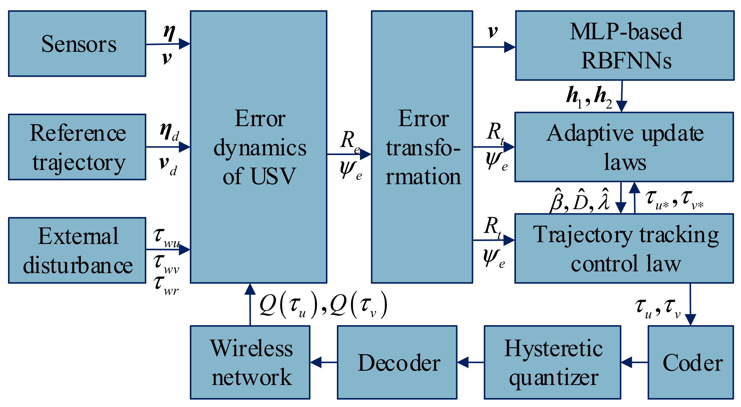
The structure of the trajectory tracking control system of USV is shown as Figure 1. To promote the controller design, several assumptions and the relevant lemma are given as:

Assumption 1.

The reference trajectories in (9) should be smooth—that is, $x_d$, $y_d$, ${\psi }_d$, ${\dot{x}}_d$, ${\dot{y}}_d$, and ${\dot{\psi }}_d$are all bounded.

Assumption 2.

The external disturbance, ${\tau }_{wu}$, ${\tau }_{wv}$, and ${\tau }_{wr}$, are unknown but bounded—that is, ${\tau }_{wu}\le d_u$, ${\tau }_{wv}\le d_v$, and ${\tau }_{wr}\le d_r$hold with $d_u,d_v,d_r$in being unknown positive constants.

Lemma 3.

[35]: For any $\epsilon >0$ and $x\in ℝ$, the following inequality holds:

$$0\le \left|x\right|-\frac{{\left|x\right|}^2}{\sqrt{x^2+{\epsilon }^2}}\le \left|x\right|-\frac{{\left|x\right|}^2}{\left|x\right|+\epsilon }<\epsilon$$

(12)

The control objective of this study can be summarized as follows. The backstepping filtering algorithm is constructed for the trajectory tracking control of underactuated USVs. On the basis of Assumptions 1 and 2, the constrained communication bandwidth and system uncertainties are taken into consideration. Consequently, the position and attitude tracking errors are stabilized, while the predefined transient performance is guaranteed.

3. Adaptive Backstepping Design Based on Quantized Input

In this section, a quantized prescribed performance control strategy is provided for the trajectory tracking of an underactuated USV. Aiming at stabilizing the position and attitude tracking errors, the backstepping-based dynamic filtering method is developed with compensation for EOC. In particular, the accurate approximation for unmeasured parameters is implemented via MLP algorithm-based RBFNNs, which have a low burden of computational resources. Meanwhile, with the consideration of the constrained communication bandwidth between controllers and actuators, the HLQ is introduced to provide the quantized control signal and the resulting quantization errors are eliminated by resorting to the adaptive estimation.

3.1. Position Controller Design

When reviewing the tracking errors defined in (10), it follows that:

$$x_e=R_e\cos \left({\psi }_r\right),y_e=R_e\sin \left({\psi }_r\right)$$

(13)

Taking into account (1) and (9), the time derivative of $R_e$ can be obtained as:

$$\begin{array}{cc}{\dot{R}}_e\hfill & = \left(x_e{\dot{x}}_e+y_e{\dot{y}}_e\right)/R_e\hfill \\ & = \left({\dot{x}}_d-\dot{x}\right)\cos \left({\psi }_r\right)+\left({\dot{y}}_d-\dot{y}\right)\sin \left({\psi }_r\right)\hfill \\ & = \left({\dot{x}}_d-u\cos \left(\psi \right)+v\sin \left(\psi \right)\right)\cos \left({\psi }_r\right)+\left({\dot{y}}_d-u\sin \left(\psi \right)-v\cos \left(\psi \right)\right)\sin \left({\psi }_r\right)\hfill \\ & = {\dot{x}}_d\cos \left({\psi }_r\right)+{\dot{y}}_d\sin \left({\psi }_r\right)-u\cos \left({\psi }_e\right)-v\sin \left({\psi }_e\right)\hfill \end{array}$$

(14)

To ensure that the tracking error dynamics satisfy the designer-specified behavioral metrics, the error transformation is executed [37] so that an equivalent “state-constrained” model is established for the subsequent controller design. First off, a positive continue function, $b_1(t)$, is introduced as the upper bound of $R_e$, which means:

$$\left|R_e\right| \le b_1\left(t\right)$$

(15)

with the performance function (PF) $b_1\left(t\right)$ satisfying $b_1\left(0\right) > R_e\left(0\right)$. Furthermore, the normalized tracking error (NTE) is expressed as:

$$R_n=\frac{R_e}{b_1}$$

(16)

By resorting to the tangent function, the error transformation equation is defined as:

$$R_t=\tan \left(\frac{\pi R_n}{2}\right)$$

(17)

Remark 4.

Mathematically, if $\left|R_e\right|\to b_1\left(t\right)$, it has $R_n\to 1$(or $R_n\to -1$); thus, $R_t\to \infty$(or $R_t\to -\infty$) holds and vice versa. In other words, the performance constraint (15) can be satisfied through bounding the variable $R_t$. Consequently, the control objective of position tracking designs an algorithm to guarantee the boundedness and convergence of $R_t$.

According to (14), the derivative of $R_n$ and $R_t$ can be obtained as:

$${\dot{R}}_n=\frac{{\dot{R}}_e{b}_1-R_e{\dot{b}}_1}{b_1^2}=\frac{1}{b_1}\left(-R_n{\dot{b}}_1+{\dot{x}}_d\cos \left({\psi }_r\right)+{\dot{y}}_d\sin \left({\psi }_r\right)-u\cos \left({\psi }_e\right)-v\sin \left({\psi }_e\right)\right)$$

(18)

$${\dot{R}}_t={\mathsf{\Gamma }}_R\left(-R_n{\dot{b}}_1+{\dot{x}}_d\cos \left({\psi }_r\right)+{\dot{y}}_d\sin \left({\psi }_r\right)-u\cos \left({\psi }_e\right)-v\sin \left({\psi }_e\right)\right)$$

(19)

where ${\mathsf{\Gamma }}_R=\frac{\pi \left(1+R_t^2\right)}{2b_1}$ is a positive definite variable.

Step 1. With the definition of the velocity tracking error $u_e=u_d-u$, the Lyapunov function candidate (LFC) is selected as:

$$V_1=\frac{1}{2}{R}_t^2$$

(20)

Taking the time derivative of $V_1$ and substituting (19) yields:

$$\begin{array}{cc}{\dot{V}}_1\hfill & =R_t{\dot{R}}_t\hfill \\ & ={\mathsf{\Gamma }}_R{R}_t\left(-R_n{\dot{b}}_1+{\dot{x}}_d\cos \left({\psi }_r\right)+{\dot{y}}_d\sin \left({\psi }_r\right)-u\cos \left({\psi }_e\right)-v\sin \left({\psi }_e\right)\right)\hfill \\ & ={\mathsf{\Gamma }}_R{R}_t\left[-R_n{\dot{b}}_1+{\dot{x}}_d\cos \left({\psi }_r\right)+{\dot{y}}_d\sin \left({\psi }_r\right)-u_d\cos \left({\psi }_e\right)+u_e\cos \left({\psi }_e\right)-v\sin \left({\psi }_e\right)\right]\hfill \end{array}$$

(21)

To stabilize the transformed position tracking error $R_t$, the virtual control law $u_d$ is proposed as:

$$u_d=\frac{1}{\cos \left({\psi }_e\right)}\left(k_1{R}_t-R_n{\dot{b}}_1+{\dot{x}}_d\cos \left({\psi }_r\right)+{\dot{y}}_d\sin \left({\psi }_r\right)-v\sin \left({\psi }_e\right)\right)$$

(22)

with the design parameter $k_1$ being a positive constant.

Substituting it into (21), ${\dot{V}}_1$ becomes:

$${\dot{V}}_1={\mathsf{\Gamma }}_R{R}_t\left(-k_1{R}_t+u_e\cos \left({\psi }_e\right)\right)$$

(23)

Step 2. To remedy the problem of the EOC, a first-order low-pass filter is introduced to process the virtual command $u_d$. The output characteristic of the filter is given as:

$$\begin{array}{l}{l}_1{\dot{u}}_c+u_c=u_d,u_c\left(0\right)=u_d\left(0\right)\\ {\dot{u}}_c=\left(u_d-u_c\right)/{\iota }_1\end{array}$$

(24)

where $u_c$ is the output signal and the constant ${\iota }_1$ is the filter parameter. Thus, in the following design ${\dot{u}}_d$ is replaced by ${\dot{u}}_c$. The second LFC is chosen as:

$$V_2=V_1+\frac{1}{2}{u}_e^2$$

(25)

According to the dynamic (2) and the result (23), the derivative of $V_2$ is written as:

$$\begin{array}{cc}{\dot{V}}_2\hfill & ={\dot{V}}_1+u_e{\dot{u}}_e\hfill \\ & ={\mathsf{\Gamma }}_R{R}_t\left(-k_1{R}_t+u_e\cos \left({\psi }_e\right)\right)+u_e\left({\dot{u}}_c-\dot{u}\right)\hfill \\ & ={\mathsf{\Gamma }}_R{R}_t\left(-k_1{R}_t+u_e\cos \left({\psi }_e\right)\right)\hfill \\ & +u_e\left({\dot{u}}_c-\frac{m_{22}}{m_{11}}v\omega -\frac{1}{m_{11}}Q\left({\tau }_u\right)+f_u\left(u\right)-\frac{1}{m_{11}}{\tau }_{wu}\right)\hfill \end{array}$$

(26)

In particular, the hydrodynamic damping term $f_u\left(u\right)$ is regarded as an unknown continuous function that can be approximated by RBFNN. Learning from Lemma 2, one finds:

$$f_u\left(u\right)=W_1^{\mathrm{T}}{h}_1\left(v\right)+o_1$$

(27)

where the approximation error $o_1$ satisfies $0<o_1\le O_1$.

In order to remove the need for the excessive calculations caused by estimating the entire weight matrix, the upper bound ${\beta }_1$ is introduced as ${\beta }_1\ge ‖W_1‖$ and the parameter $h_1$ is defined as $h_1=‖h_1\left(v\right)‖$. Hence, ${\dot{V}}_2$ can be further derived as:

$$\begin{array}{cc}{\dot{V}}_2\hfill & ={\mathsf{\Gamma }}_R{R}_t\left(-k_1{R}_t+u_e\cos \left({\psi }_e\right)\right)+u_e\left({\dot{u}}_c-\frac{m_{22}}{m_{11}}v\omega -\frac{1}{m_{11}}Q\left({\tau }_u\right)\right)\hfill \\ & +u_e\left(W_1^{\mathrm{T}}{h}_1\left(v\right)+o_1-\frac{1}{m_{11}}{\tau }_{wu}\right)\hfill \\ & \le {\mathsf{\Gamma }}_R{R}_t\left(-k_1{R}_t+u_e\cos \left({\psi }_e\right)\right)+u_e\left({\dot{u}}_c-\frac{m_{22}}{m_{11}}v\omega -\frac{1}{m_{11}}Q\left({\tau }_u\right)\right)\hfill \\ & +\left|u_e\right|\left({\beta }_1{h}_1+O_1+\frac{1}{m_{11}}{d}_u\right)\hfill \end{array}$$

(28)

Referring to the discussion in (11, 12), the quantized signal of the control input ${\tau }_u$ can be obtained as:

$$Q\left({\tau }_u\right)={\kappa }_1\left({\tau }_u\right){\tau }_u-E_1\left({\tau }_u\right)$$

(29)

with $1-{\delta }_1\le {\kappa }_1\left({\tau }_u\right) \le 1+{\delta }_1$ and $E_1\left({\tau }_u\right) \le {\tau }_{\mathrm{umin}}$.

To facilitate the adaptive estimation, it is defined that ${\lambda }_1=\frac{1}{1-{\delta }_1}$ and $D_1=O_1+\frac{1}{m_{11}}{d}_u+\frac{1}{m_{11}}{\tau }_{\mathrm{umin}}$. Moreover, the variables ${\widehat{\beta }}_1$, ${\widehat{D}}_1$, and ${\widehat{\lambda }}_1$ are introduced as estimate values, while the estimate errors are represented as ${\tilde{\beta }}_1$, ${\tilde{D}}_1$, and ${\tilde{\lambda }}_1$.

$${\tilde{\beta }}_1={\beta }_1-{\widehat{\beta }}_1,{\tilde{D}}_1=D_1-{\widehat{D}}_1,{\tilde{\lambda }}_1={\lambda }_1-{\widehat{\lambda }}_1$$

(30)

Subsequently, the control signal is constructed as:

$${\tau }_u=m_{11}{\widehat{\lambda }}_1{\tau }_{u\ast }$$

(31)

$${\tau }_{u\ast }=\frac{{\eta }_t^2{u}_e}{\sqrt{{\eta }_t^2{u}_{\mathrm{e}}^2+{\epsilon }_1}}+\left(k_2+k_u\right)u_e$$

(32)

$$k_u=\frac{{\widehat{\beta }}_1^2{h}_1^2}{\sqrt{{\widehat{\beta }}_1^2{h}_1^2{u}_e^2+{\epsilon }_1}}+\frac{{\widehat{D}}_1^2}{\sqrt{{\widehat{D}}_1^2{u}_{\mathrm{e}}^2+{\epsilon }_1}}$$

(33)

where ${\eta }_t=\left({\dot{u}}_c-\frac{m_{22}}{m_{11}}vr+{\mathsf{\Gamma }}_R{R}_t\cos \left({\psi }_e\right)\right)$ and the controller parameter $k_2$ is a positive constant. Furthermore, the adaptive update laws are given as:

$${\dot{\widehat{\beta }}}_1=c_1\left(h_1\left|u_e\right|-c_2{\widehat{\beta }}_1\right)$$

(34)

$${\dot{\widehat{D}}}_1=c_3\left(\left|u_e\right|-c_4{\widehat{D}}_1\right)$$

(35)

$${\dot{\widehat{\lambda }}}_1=c_5\left(u_e{\tau }_{u\ast }-c_6{\widehat{\lambda }}_1\right)$$

(36)

where $c_i\left(i=1,2,3,4,5,6\right)$ are all positive parameters.

Remark 5.

Considering the ingeniously designed controller (31–34), there exist three highlights that deserve some attention. (i) Different from the conservative quantized control, the algorithm introduced in this paper is developed under the unavailable quantizer parameter${\delta }_1$. For this reason, the constant${\lambda }_1$is introduced for adaptive estimation and procedure (31) is constructed to compensate the resulting concussion. (ii) The unknown constant$D_1$is defined as the lumped additive uncertainties, which is constituted by the approximation error of NN, the environmental disturbance, and the hysteresis zone of the quantizer. On the other hand, the scalar${\beta }_1$is utilized for estimating the weight matrix of RBFNN, which emphatically reflects the superiority of MLP in terms of the computation burden. (iii) The first term in${\tau }_{u\ast }$stands for system dynamics compensation, and the remainder suppresses the phenomenon of chattering, while the convergence of tracking errors and estimate errors can be ensured.

For the sake of convenience, ${\kappa }_1\left({\tau }_u\right)$ and $E_1\left({\tau }_u\right)$ are abbreviated as ${\kappa }_1$ and $E_1$, respectively. Thus, with the substitution of (29), (28) can be further written as:

$$\begin{array}{cc}{\dot{V}}_2\hfill & \le {\mathsf{\Gamma }}_R{R}_t\left(-k_1{R}_t+u_e\cos \left({\psi }_e\right)\right)+u_e\left[{\dot{u}}_c-\frac{m_{22}}{m_{11}}vr-\frac{1}{m_{11}}\left({\kappa }_1{\tau }_u-E_1\right)\right]\hfill \\ & +\left|u_e\right|\left({\beta }_1{h}_1+O_1+\frac{1}{m_{11}}{d}_u\right)\hfill \end{array}$$

(37)

According to the property of ${\kappa }_1$, ${\lambda }_1$ and substituting (31), the term $-\frac{1}{m_{11}}\left({\kappa }_1{\tau }_u-E_1\right)$ can be calculated as:

$$\begin{array}{cc}-\frac{1}{m_{11}}\left({\kappa }_1{\tau }_u-E_1\right)u_e\hfill & =-\frac{1}{m_{11}}\left({\kappa }_1{m}_{11}\widehat{\lambda }{\tau }_{u\ast }-E_1\right)u_e\hfill \\ & =-{\kappa }_1\left({\lambda }_1-{\tilde{\lambda }}_1\right)u_e{\tau }_{u\ast }+\frac{1}{m_{11}}{E}_1{u}_e\hfill \\ & \le -\left(1-{\delta }_1\right)\left({\lambda }_1-{\tilde{\lambda }}_1\right)u_e{\tau }_{u\ast }+\frac{1}{m_{11}}{E}_1{u}_e\hfill \\ & =-u_e{\tau }_{u\ast }+\left(1-{\delta }_1\right){\tilde{\lambda }}_1{u}_e{\tau }_{u\ast }+\frac{1}{m_{11}}{\tau }_{\mathrm{umin}}\left|u_e\right|\hfill \end{array}$$

(38)

By recalling the control signal in (32) and utilizing Lemma 3, one finds:

$$\begin{array}{cc}-\frac{1}{m_{11}}\left({\kappa }_1{\tau }_u-E_1\right)u_e\hfill & \le \left(1-{\delta }_1\right){\tilde{\lambda }}_1{u}_e{\tau }_{u\ast }+\frac{1}{m_{11}}{E}_1{u}_e-u_e\left(\frac{{\eta }_t^2{u}_e}{\sqrt{{\eta }_t^2{u}_{\mathrm{e}}^2+{\epsilon }_1}}+\left(k_2+k_u\right)u_e\right)\hfill \\ & \le -\left|{\eta }_t{u}_e\right|-\left(k_2+k_u\right)u_e^2+\left(1-{\delta }_1\right){\tilde{\lambda }}_1{u}_e{\tau }_{u\ast }+\frac{1}{m_{11}}{\tau }_{\mathrm{umin}}\left|u_e\right|+{\epsilon }_1\hfill \end{array}$$

(39)

Substituting the result into (37), ${\dot{V}}_2$ can be scaled as:

$$\begin{array}{cc}{\dot{V}}_2\hfill & \le {\mathsf{\Gamma }}_R{R}_t\left(-k_1{R}_t+u_e\cos \left({\psi }_e\right)\right)+u_e\left({\dot{u}}_c-\frac{m_{22}}{m_{11}}v\omega \right)\hfill \\ & -\left|\left({\dot{u}}_c-\frac{m_{22}}{m_{11}}vr+{\mathsf{\Gamma }}_R{R}_t\cos \left({\psi }_e\right)\right)u_e\right|-\left(k_2+k_u\right)u_e^2\hfill \\ & +\left(1-{\delta }_1\right){\tilde{\lambda }}_1{u}_e{\tau }_{u\ast }+\left|u_e\right|{\beta }_1{h}_1+\left|u_e\right|\left(O_1+\frac{1}{m_{11}}{d}_u+\frac{1}{m_{11}}{\tau }_{\mathrm{umin}}\right)+{\epsilon }_1\hfill \\ & \le -k_1{\mathsf{\Gamma }}_R{R}_t^2-\left(k_2+k_u\right)u_e^2+\left(1-{\delta }_1\right){\tilde{\lambda }}_1{u}_e{\tau }_{u\ast }+\left|u_e\right|{\beta }_1{h}_1+\left|u_e\right|D_1+{\epsilon }_1\hfill \end{array}$$

(40)

Consequently, taking into account (33), a concise result can be obtained:

$$\begin{array}{cc}{\dot{V}}_2\hfill & \le -k_1{\Gamma }_R{R}_t^2-k_2{u}_e^2-u_e^2\left(\frac{{\widehat{\beta }}_1^2{h}_1^2}{\sqrt{{\widehat{\beta }}_1^2{h}_1^2{u}_{\mathrm{e}}^2+{\epsilon }_1}}+\frac{{\widehat{D}}_1^2}{\sqrt{{\widehat{D}}_1^2{u}_{\mathrm{e}}^2+{\epsilon }_1}}\right)\hfill \\ & +\left(1-{\delta }_1\right){\tilde{\lambda }}_1{u}_e{\tau }_{u\ast }+\left|u_e\right|{\beta }_1{h}_1+\left|u_e\right|D_1+{\epsilon }_1\hfill \\ & \le -k_1{\Gamma }_R{R}_t^2-k_2{u}_e^2-\left|u_e\right|{\widehat{\beta }}_1{h}_1-\left|u_e\right|{\widehat{D}}_1+\left(1-{\delta }_1\right){\tilde{\lambda }}_1{u}_e{\tau }_{u\ast }+\left|u_e\right|{\beta }_1{h}_1+\left|u_e\right|D_1+2{\epsilon }_1\hfill \\ & =-k_1{\Gamma }_R{R}_t^2-k_2{u}_e^2+\left|u_e\right|{\tilde{\beta }}_1{h}_1+\left|u_e\right|{\tilde{D}}_1+\left(1-{\delta }_1\right){\tilde{\lambda }}_1{u}_e{\tau }_{u\ast }+2{\epsilon }_1\hfill \end{array}$$

(41)

3.2. Attitude Controller Design

According to (10), the derivative of ${\psi }_e$ is expressed as:

$${\dot{\psi }}_e={\dot{\psi }}_r-r$$

(42)

Step 1. To stabilize the attitude of the pursuer, the LFC is selected as:

$$V_3=\frac{1}{2}{\psi }_e^2$$

(43)

With the definition of the angular velocity tracking error being $r_e=r_d-r$, the time derivative of (44) is deduced as:

$$\begin{array}{cc}{\dot{V}}_3\hfill & ={\psi }_e{\dot{\psi }}_e\hfill \\ & ={\psi }_e\left({\dot{\psi }}_r-r\right)\hfill \\ & ={\psi }_e\left({\dot{\psi }}_r+r_e-r_d\right)\hfill \end{array}$$

(44)

Specially, the virtual control law $r_d$ is designed as:

$$r_d=k_3{\psi }_e+{\dot{\psi }}_r$$

(45)

with $k_3$ being a positive constant. Hence, ${\dot{V}}_3$ becomes:

$${\dot{V}}_3={\psi }_e\left(r_e-k_3{\psi }_e\right)$$

(46)

Step 2. Referring to (24), let the virtual control law $r_d$ pass through a first-order filter:

$$\begin{array}{l}{\iota }_2{\dot{r}}_c+r_c=r_d,r_c\left(0\right)=r_d\left(0\right)\\ {\dot{r}}_c=\left(r_d-r_c\right)/{\iota }_2\end{array}$$

(47)

where $r_c$ is the filtered signal and ${\iota }_2$ is the filter parameter. In this step, ${\dot{r}}_d$ is substituted by ${\dot{r}}_c$.

$$V_4=V_3+\frac{1}{2}{r}_e^2$$

(48)

Differentiating $V_4$ with respect to time and substituting (10), one obtains:

$$\begin{array}{cc}{\dot{V}}_4\hfill & ={\dot{V}}_3+r_e{\dot{r}}_e\hfill \\ & ={\psi }_e\left(r_e-k_3{\psi }_e\right)+r_e\left({\dot{r}}_c-\dot{r}\right)\hfill \\ & ={\psi }_e\left(r_e-k_3{\psi }_e\right)+r_e\left({\dot{r}}_c-\frac{m_{11}-m_{22}}{m_{33}}uv-\frac{1}{m_{33}}Q\left({\tau }_r\right)+f_r\left(r\right)-\frac{1}{m_{33}}{\tau }_{wr}\right)\hfill \end{array}$$

(49)

One caveat here is that the nonlinear function $f_r\left(r\right)$ cannot be observed accurately. Therefore, the MLP-based RBFNN is applied to approximate the time-varying dynamics. According to Lemma 2, the following equation is valid.

$$f_r\left(r\right)=W_2^{\mathrm{T}}{h}_2\left(v\right)+o_2$$

(50)

where the approximation error satisfies $0<o_2\le O_2$. Moreover, two parameters are defined as ${\beta }_2\ge ‖W_2‖$ and $h_2=‖h_2\left(v\right)‖$, meaning that only one scalar needs to be adaptively estimated, which reduces the computational burden. In this way, (50) can be derived as:

$$\begin{array}{cc}{\dot{V}}_4\hfill & ={\psi }_e\left(r_e-k_3{\psi }_e\right)+r_e\left({\dot{r}}_c-\frac{m_{11}-m_{22}}{m_{33}}uv-\frac{1}{m_{33}}Q\left({\tau }_R\right)+W_2^{\mathrm{T}}{h}_2\left(v\right)+o_2-\frac{1}{m_{33}}{\tau }_{wr}\right)\hfill \\ & \le {\psi }_e\left(r_e-k_3{\psi }_e\right)+r_e\left({\dot{r}}_c-\frac{m_{11}-m_{22}}{m_{33}}uv-\frac{1}{m_{33}}Q\left({\tau }_R\right)\right)+\left|r_e\right|\left({\beta }_2{h}_2+O_2+\frac{1}{m_{33}}{d}_r\right)\hfill \end{array}$$

(51)

Learning from Lemma 1, the quantized signal for control input ${\tau }_r$ can be written as:

$$Q\left({\tau }_r\right)={\kappa }_2\left({\tau }_r\right){\tau }_r-E_2\left({\tau }_r\right)$$

(52)

with $1-{\delta }_2\le {\kappa }_2\left({\tau }_r\right)\le 1+{\delta }_2$ and $E_2\left({\tau }_r\right)\le {\tau }_{\mathrm{rmin}}$.

Before giving the control algorithm, it is necessary to define the parameter ${\lambda }_2=\frac{1}{1-{\delta }_2}$ and the lumped unknown term $D_2=O_2+\frac{1}{m_{33}}{d}_r+\frac{1}{m_{33}}{\tau }_{\mathrm{rmin}}$. Meanwhile, the adaptive estimate values are introduced as ${\widehat{D}}_2$, ${\widehat{\beta }}_2$, and ${\widehat{\lambda }}_2$, meaning that the estimate errors can be expressed as:

$${\tilde{D}}_2=D_2-{\widehat{D}}_2,{\tilde{\beta }}_2={\beta }_2-{\widehat{\beta }}_2,{\tilde{\lambda }}_2={\lambda }_2-{\widehat{\lambda }}_2$$

(53)

Consequently, the control input is elaborated as:

$${\tau }_r=m_{33}{\widehat{\lambda }}_2{\tau }_{r\ast }$$

(54)

$${\tau }_{r\ast }=\frac{{\eta }_r^2{r}_e}{\sqrt{{\eta }_r^2{r}_{\mathrm{e}}^2+{\epsilon }_2}}+\left(k_4+k_r\right)r_e$$

(55)

$$k_r=\frac{{\widehat{\beta }}_2^2{h}_2^2}{\sqrt{{\widehat{\beta }}_2^2{h}_2^2{r}_{\mathrm{e}}^2+{\epsilon }_2}}+\frac{{\widehat{D}}_2^2}{\sqrt{{\widehat{D}}_2^2{r}_{\mathrm{e}}^2+{\epsilon }_2}}$$

(56)

where ${\eta }_r=\left({\dot{r}}_c-\frac{m_{11}-m_{22}}{m_{33}}uv+{\psi }_e\right)$; $k_4$ is a positive controller parameter. The adaptive learning laws are given as:

$${\dot{\widehat{\beta }}}_2=c_7\left(h_2\left|r_e\right|-c_8{\widehat{\beta }}_2\right)$$

(57)

$${\dot{\widehat{D}}}_2=c_9\left(\left|r_e\right|-c_{10}{\widehat{D}}_2\right)$$

(58)

$${\dot{\widehat{\lambda }}}_2=c_{11}\left(r_e{\tau }_{r\ast }-c_{12}{\widehat{\lambda }}_2\right)$$

(59)

where $c_i\left(i=7,8,9,10,11,12\right)$ are all positive constants.

According to the definitions of ${\kappa }_2$ and ${\lambda }_2$, the term $-\frac{1}{m_{33}}\left({\kappa }_2{\epsilon }_{\omega }-E_2\right)$ can be calculated as:

$$\begin{array}{cc}-\frac{1}{m_{33}}\left({\kappa }_2{\tau }_r-E_2\right)r_e\hfill & =-\frac{1}{m_{33}}\left({\kappa }_2{m}_{33}{\widehat{\lambda }}_2{\tau }_r-E_2\right)r_e\hfill \\ & =-{\kappa }_2{\widehat{\lambda }}_2{r}_e{\tau }_r+\frac{1}{m_{33}}{E}_2{r}_e\hfill \\ & \le -\left(1-{\delta }_2\right)\left({\lambda }_2-{\tilde{\lambda }}_2\right)r_e{\tau }_r+\frac{1}{m_{33}}{E}_2{r}_e\hfill \\ & =-{\epsilon }_r{r}_e+\left(1-{\delta }_2\right){\tilde{\lambda }}_2{r}_e{\tau }_r+\frac{1}{m_{33}}{\tau }_{\mathrm{rmin}}{r}_e\hfill \end{array}$$

(60)

Substituting the control signal in (55) leads to:

$$\begin{array}{cc}-\frac{1}{m_{33}}\left({\kappa }_2{\tau }_r-E_2\right)r_e\hfill & \le -\frac{{\eta }_r^2{r}_{\mathrm{e}}^2}{\sqrt{{\eta }_r^2{r}_{\mathrm{e}}^2+{\epsilon }_2}}-\left(k_4+k_{\omega }\right)r_{\mathrm{e}}^2+\left(1-{\delta }_2\right){\tilde{\lambda }}_2{r}_e{\tau }_r+\frac{1}{m_{33}}{\tau }_{\mathrm{rmin}}{r}_e\hfill \\ & \le -\left|{\eta }_r{r}_e\right|-\left(k_4+k_r\right)r_{\mathrm{e}}^2+\left(1-{\delta }_2\right){\tilde{\lambda }}_2{r}_e{\tau }_r+\frac{1}{m_{33}}{\tau }_{\mathrm{rmin}}{r}_e+{\epsilon }_2\hfill \end{array}$$

(61)

Taking the results into consideration, (52) follows:

$$\begin{array}{cc}{\dot{V}}_4\hfill & \le {\psi }_e\left(r_e-k_3{\psi }_e\right)+r_e\left({\dot{r}}_c-\frac{m_{11}-m_{22}}{m_{33}}uv\right)-\left|\left({\dot{r}}_c-\frac{m_{11}-m_{22}}{m_{33}}uv+{\psi }_e\right)r_e\right|\hfill \\ & -\left(k_4+k_r\right)r_{\mathrm{e}}^2+\left(1-{\delta }_2\right){\tilde{\lambda }}_2{r}_e{\tau }_r+\left|r_e\right|{\beta }_2{h}_2+\left|r_e\right|\left(O_2+\frac{1}{m_{33}}{d}_r+\frac{1}{m_{33}}{\tau }_{\mathrm{rmin}}\right)\hfill \\ & \le -k_3{\psi }_e^2-\left(k_4+k_r\right)r_{\mathrm{e}}^2+\left(1-{\delta }_2\right){\tilde{\lambda }}_2{r}_e{\tau }_r+\left|r_e\right|{\beta }_2{h}_2+\left|r_e\right|D_2\hfill \end{array}$$

(62)

Finally, with the substitution of (57), a concise result is obtained:

$$\begin{array}{cc}{\dot{V}}_4\hfill & \le -k_3{\psi }_e^2-k_4{r}_{\mathrm{e}}^2-r_{\mathrm{e}}^2\left(\frac{{\widehat{\beta }}_2^2{h}_2^2}{\sqrt{{\widehat{\beta }}_2^2{h}_2^2{r}_{\mathrm{e}}^2+{\epsilon }_2}}+\frac{{\widehat{D}}_2^2}{\sqrt{{\widehat{D}}_2^2{r}_{\mathrm{e}}^2+{\epsilon }_2}}\right)\hfill \\ & +\left(1-{\delta }_2\right){\tilde{\lambda }}_2{r}_e{\tau }_r+\left|r_e\right|{\beta }_2{h}_2+\left|r_e\right|D_2\hfill \\ & \le -k_3{\psi }_e^2-k_4{r}_{\mathrm{e}}^2-\left|r_e\right|{\widehat{\beta }}_2{h}_2-\left|r_e\right|{\widehat{D}}_2+\left(1-{\delta }_2\right){\tilde{\lambda }}_2{r}_e{\tau }_r+\left|r_e\right|{\beta }_2{h}_2+\left|r_e\right|D_2+2{\epsilon }_2\hfill \\ & =-k_3{\psi }_e^2-k_4{r}_{\mathrm{e}}^2+\left|r_e\right|{\tilde{\beta }}_2{h}_2+\left|r_e\right|{\tilde{D}}_2+\left(1-{\delta }_2\right){\tilde{\lambda }}_2{r}_e{\tau }_r+2{\epsilon }_2\hfill \end{array}$$

(63)

3.3. Stability Analysis

In this section, the stability analysis proceeds using the Lyapunov theory. First off, the theorem is given as follows.

Theorem 1.

Consider the underactuated AUV model described in (1) and (2) and the tracking error dynamics (14) under Assumptions 1 and 2. On basis of the quantizer (4), the error transformation (21), the filters (24) and (48), and the controllers (31)–(36) and (55)–(60) are capable of ensuring that all signals in the closed-loop system are bounded and that the position tracking error$R_e$satisfies the predefined behavioral metrics.

Proof. 

In order to prevent the adverse effects caused by the introduction of filters, the filter errors are defined and the validation will be provided to guarantee their convergence.

$${\tilde{\alpha }}_u=u_c-u_d,{\tilde{\alpha }}_r=r_c-r_d$$

(64)

Associated with the descriptions of (24) and (48), their time derivatives satisfy the relation:

$$\begin{array}{l}{\dot{\tilde{\alpha }}}_u={\dot{u}}_c-{\dot{u}}_d=-\frac{{\tilde{\alpha }}_u}{{\iota }_1}+{\dot{u}}_d\le -\frac{{\tilde{\alpha }}_u}{{\iota }_1}+B_1,\\ {\dot{\tilde{\alpha }}}_r={\dot{r}}_c-{\dot{r}}_d=-\frac{{\tilde{\alpha }}_r}{{\iota }_2}+{\dot{r}}_d\le -\frac{{\tilde{\alpha }}_r}{{\iota }_2}+B_2.\end{array}$$

(65)

where the continuous function $B_i\left(i=1,2\right)$ possesses an unknown certain maximum—i.e., $\left|B_i\right|\le {\vartheta }_i$.

Subsequently, the overall LFC is defined as:

$$\begin{array}{l}V=V_2+\frac{1}{2c_1}{\tilde{\beta }}_1^2+\frac{1}{2c_3}{\tilde{D}}_1^2+\frac{1-{\delta }_1}{2c_5}{\tilde{\lambda }}_1^2+\frac{1}{2}{\tilde{\alpha }}_u^2\\ \hspace{0.33em}\hspace{0.33em}\hspace{0.33em}\hspace{0.33em}+V_4+\frac{1}{2c_7}{\tilde{\beta }}_2^2+\frac{1}{2c_9}{\tilde{D}}_2^2+\frac{1-{\delta }_2}{2{\gamma }_{11}}{\tilde{\lambda }}_2^2+\frac{1}{2}{\tilde{\alpha }}_r^2\end{array}$$

(66)

With the aid of (41) and (63), differentiating $V$ with respect to time yields:

$$\begin{array}{cc}\dot{V}\hfill & ={\dot{V}}_1+\frac{1}{c_1}{\tilde{\beta }}_1{\dot{\tilde{\beta }}}_1+\frac{1}{c_3}{\tilde{D}}_1{\dot{\tilde{D}}}_1+\frac{1-{\delta }_1}{{\gamma }_2}{\tilde{\lambda }}_1{\dot{\tilde{\lambda }}}_1+{\tilde{\alpha }}_u{\dot{\tilde{\alpha }}}_u\hfill \\ & +{\dot{V}}_2+\frac{1}{c_5}{\tilde{\beta }}_2{\dot{\tilde{\beta }}}_2+\frac{1}{c_7}{\tilde{D}}_2{\dot{\tilde{D}}}_2+\frac{1-{\delta }_2}{{\gamma }_6}{\tilde{\lambda }}_2{\dot{\tilde{\lambda }}}_2+{\tilde{\alpha }}_r{\dot{\tilde{\alpha }}}_r\hfill \\ & =-k_1{\Gamma }_R{R}_t^2-k_2{u}_e^2+\left|u_e\right|{\tilde{\beta }}_1{h}_1+\left|u_e\right|{\tilde{D}}_1+\left(1-{\delta }_1\right){\tilde{\lambda }}_1{u}_e{\tau }_{u\ast }+2{\epsilon }_1\hfill \\ & -{\tilde{\beta }}_1\left(h_1\left|u_e\right|-c_2{\widehat{\beta }}_1\right)-{\tilde{D}}_1\left(\left|u_e\right|-c_4{\widehat{D}}_1\right)-\left(1-{\delta }_1\right){\tilde{\lambda }}_1\left(u_e{\tau }_{u\ast }-c_6{\widehat{\lambda }}_1\right)+{\tilde{\alpha }}_u{\dot{\tilde{\alpha }}}_u\hfill \\ & -k_3{\psi }_e^2-k_4{r}_{\mathrm{e}}^2+\left|r_e\right|{\tilde{\beta }}_2{h}_2+\left|r_e\right|{\tilde{D}}_2+\left(1-{\delta }_2\right){\tilde{\lambda }}_2{r}_e{\tau }_r+2{\epsilon }_2\hfill \\ & -{\tilde{\beta }}_2\left(h_2\left|r_e\right|-c_8{\widehat{\beta }}_2\right)-{\tilde{D}}_2\left(\left|r_e\right|-c_{10}{\widehat{D}}_2\right)-\left(1-{\delta }_2\right){\tilde{\lambda }}_2\left(r_e{\tau }_{r\ast }-c_{12}{\widehat{\lambda }}_2\right)+{\tilde{\alpha }}_r{\dot{\tilde{\alpha }}}_r\hfill \\ & =-k_1{\Gamma }_R{R}_t^2-k_2{u}_e^2+c_2{\widehat{\beta }}_1{\tilde{\beta }}_1+c_4{\widehat{D}}_1{\tilde{D}}_1+c_6\left(1-{\delta }_1\right){\widehat{\lambda }}_1{\tilde{\lambda }}_1+{\tilde{\alpha }}_u{\dot{\tilde{\alpha }}}_u+2{\epsilon }_1\hfill \\ & -k_3{\psi }_e^2-k_4{r}_{\mathrm{e}}^2+c_8{\widehat{\beta }}_2{\tilde{\beta }}_2+c_{10}{\widehat{D}}_2{\tilde{D}}_2+c_{12}\left(1-{\delta }_2\right){\widehat{\lambda }}_2{\tilde{\lambda }}_2+{\tilde{\alpha }}_r{\dot{\tilde{\alpha }}}_r+2{\epsilon }_2\hfill \end{array}$$

(67)

By resorting to Young’s inequality, one of the above terms can be scaled as:

$$\begin{array}{cc}{c}_2{\widehat{\beta }}_1{\tilde{\beta }}_1\hfill & =c_2\left(-{\tilde{\beta }}_1^2+{\beta }_1{\tilde{\beta }}_1\right)\hfill \\ & \le c_2\left(-{\tilde{\beta }}_1^2+\frac{1}{2{\sigma }_1}{\tilde{\beta }}_1^2+\frac{{\sigma }_1}{2}{\beta }_1^2\right)\hfill \\ & \le -\frac{c_2\left(2{\sigma }_1-1\right)}{2{\sigma }_1}{\tilde{\beta }}_1^2+\frac{c_2{\sigma }_1}{2}{\beta }_1^2\hfill \end{array}$$

(68)

where ${\sigma }_1>0.5$. Then, a similar calculation can be implemented for $c_4{\widehat{D}}_1{\tilde{D}}_1$, $c_6\left(1-{\delta }_1\right){\widehat{\lambda }}_1{\tilde{\lambda }}_1$, $c_8{\widehat{\beta }}_2{\tilde{\beta }}_2$, $c_{10}{\widehat{D}}_2{\tilde{D}}_2$, and $c_{12}\left(1-{\delta }_2\right){\widehat{\lambda }}_2{\tilde{\lambda }}_2$, whose results are shown as:

$$\begin{array}{c}{c}_4{\widehat{D}}_1{\tilde{D}}_1\le -\frac{c_4\left(2{\sigma }_2-1\right)}{2{\sigma }_2}{\tilde{D}}_1^2+\frac{c_4{\sigma }_2}{2}{D}_1^2\\ c_6\left(1-{\delta }_1\right){\widehat{\lambda }}_1{\tilde{\lambda }}_1\le -\frac{c_6\left(1-{\delta }_1\right)\left(2{\sigma }_3-1\right)}{2{\sigma }_3}{\tilde{\lambda }}_1^2+\frac{c_6\left(1-{\delta }_1\right){\sigma }_3}{2}{\lambda }_1^2\\ c_8{\widehat{\beta }}_2{\tilde{\beta }}_2\le -\frac{c_8\left(2{\sigma }_4-1\right)}{2{\sigma }_4}{\tilde{\beta }}_2^2+\frac{c_8{\sigma }_4}{2}{\beta }_2^2\\ c_{10}{\widehat{D}}_2{\tilde{D}}_2\le -\frac{c_{10}\left(2{\sigma }_5-1\right)}{2{\sigma }_5}{\tilde{D}}_2^2+\frac{c_{10}{\sigma }_5}{2}{D}_2^2\\ c_{12}\left(1-{\delta }_2\right){\widehat{\lambda }}_2{\tilde{\lambda }}_2\le -\frac{c_{12}\left(1-{\delta }_2\right)\left(2{\sigma }_6-1\right)}{2{\sigma }_6}{\tilde{\lambda }}_2^2+\frac{c_{12}\left(1-{\delta }_2\right){\sigma }_6}{2}{\lambda }_2^2\end{array}$$

(69)

with ${\sigma }_i>0.5\left(i=2,3,4,5,6\right)$.

On the other hand, with the consideration of (65), the terms for the filter error lead to:

$$\begin{array}{c}{\tilde{\alpha }}_u{\dot{\tilde{\alpha }}}_u=-\frac{{\tilde{\alpha }}_u^2}{{\iota }_1}+{\tilde{\alpha }}_u{\dot{u}}_d\le -\frac{{\tilde{\alpha }}_u^2}{{\iota }_1}+\left|{\tilde{\alpha }}_u\right|{\vartheta }_1\le -\frac{{\tilde{\alpha }}_u^2}{{\iota }_1}+{\tilde{\alpha }}_u^2+\frac{{\vartheta }_1^2}{4},\\ {\tilde{\alpha }}_r{\dot{\tilde{\alpha }}}_r=-\frac{{\tilde{\alpha }}_r^2}{{\iota }_2}+{\tilde{\alpha }}_r{\dot{r}}_d\le -\frac{{\tilde{\alpha }}_r^2}{{\iota }_2}+\left|{\tilde{\alpha }}_r\right|{\vartheta }_2\le -\frac{{\tilde{\alpha }}_r^2}{{\iota }_2}+{\tilde{\alpha }}_r^2+\frac{{\vartheta }_2^2}{4}.\end{array}$$

(70)

Substituting the results of (68)–(70), $\dot{V}$ is finally obtained as:

$$\begin{array}{cc}\dot{V}\hfill & \le -k_1{\mathsf{\Gamma }}_R{R}_t^2-k_2{u}_e^2-\frac{c_2\left(2{\sigma }_1-1\right)}{2{\sigma }_1}{\tilde{\beta }}_1^2-\frac{c_4\left(2{\sigma }_2-1\right)}{2{\sigma }_2}{\tilde{D}}_1^2-\frac{c_6\left(1-{\delta }_1\right)\left(2{\sigma }_3-1\right)}{2{\sigma }_3}{\tilde{\lambda }}_1^2-\left(\frac{1}{{\gamma }_1}-1\right){\tilde{\alpha }}_u^2\hfill \\ & -k_3{\psi }_e^2-k_4{r}_{\mathrm{e}}^2-\frac{c_8\left(2{\sigma }_4-1\right)}{2{\sigma }_4}{\tilde{\beta }}_2^2-\frac{c_{10}\left(2{\sigma }_5-1\right)}{2{\sigma }_5}{\tilde{D}}_2^2-\frac{c_{12}\left(1-{\delta }_2\right)\left(2{\sigma }_6-1\right)}{2{\sigma }_6}{\tilde{\lambda }}_2^2-\left(\frac{1}{{\gamma }_2}-1\right){\tilde{\alpha }}_r^2\hfill \\ & +\frac{c_2{\sigma }_1}{2}{\beta }_1^2+\frac{c_4{\sigma }_2}{2}{D}_1^2+\frac{c_6\left(1-{\delta }_1\right){\sigma }_3}{2}{\lambda }_1^2+\frac{{\vartheta }_1^2}{4}+2{\epsilon }_1\hfill \\ & +\frac{c_8{\sigma }_4}{2}{\beta }_2^2+\frac{c_{10}{\sigma }_5}{2}{D}_2^2+\frac{c_{12}\left(1-{\delta }_2\right){\sigma }_6}{2}{\lambda }_2^2+\frac{{\vartheta }_2^2}{4}+2{\epsilon }_2\hfill \\ & \le -𝜌V+\Delta \hfill \end{array}$$

(71)

with

$$\begin{array}{c}\rho =\min \left\{\begin{array}{l}2k_1{\Gamma }_R,2k_2,\frac{c_1{c}_2\left(2{\sigma }_1-1\right)}{{\sigma }_1},\frac{c_3{c}_4\left(2{\sigma }_2-1\right)}{{\sigma }_2},\frac{c_5{c}_6\left(2{\sigma }_3-1\right)}{{\sigma }_3},2\left(\frac{1}{{\gamma }_1}-1\right)\\ 2k_3,2k_4,\frac{c_7{c}_8\left(2{\sigma }_4-1\right)}{{\sigma }_4},\frac{c_9{c}_{10}\left(2{\sigma }_5-1\right)}{{\sigma }_5},\frac{c_{11}{c}_{12}\left(2{\sigma }_6-1\right)}{{\sigma }_6},2\left(\frac{1}{{\gamma }_2}-1\right)\end{array}\right\}\\ \Delta =\frac{c_2{\sigma }_1}{2}{\beta }_1^2+\frac{c_4{\sigma }_2}{2}{D}_1^2+\frac{c_6\left(1-{\delta }_1\right){\sigma }_3}{2}{\lambda }_1^2+\frac{{\vartheta }_1^2}{4}+2{\epsilon }_1\hfill \\ +\frac{c_8{\sigma }_4}{2}{\beta }_2^2+\frac{c_{10}{\sigma }_5}{2}{D}_2^2+\frac{c_{12}\left(1-{\delta }_2\right){\sigma }_6}{2}{\lambda }_2^2+\frac{{\vartheta }_2^2}{4}+2{\epsilon }_2\hfill \end{array}$$

(72)

Thus far, this indicates that the transformed tracking errors, the estimate errors, and the filter errors tend to converge exponentially into a tiny neighborhood around zero. Hence, as illustrated in Remark 4, the predefined performance for the position tracking errors is guaranteed all the while.

Ultimately, the validity of Theorem 1 has been illustrated. □

4. Simulation

In this section, four simulation examples are conducted to validate the stability and exhibit the superiority of the proposed controller. First, a digital model is built on the basis of the USV’s motion dynamics and the specific parameters are set reasonably. Subsequently, the simulation results will be displayed in the form of figures, which are capable of demonstrating the detailed performance of the developed algorithm. Furthermore, the experiments under different environments and the comparison with a conservative controller provide to highlight the advantages of this work.

4.1. Parameter Setting

The vessel model parameters from [5] are adopted for numerical simulation, which are presented in

Table 1. Main parameters.

Parameter	Value	Unit	Parameter	Value	Unit
m11	1.1274	kg	dv	0.1183	kg/s
m22	1.8902	kg	dv2	0.05915	kg/m
m23	0.1278	kg/m2	dv3	0.029575	kg/m2
du	0.0358	kg/s	dr	0.0308	kg/s
du2	0.0179	kg/s	dr2	0.0154	kg/m
du3	0.00895	kg/m2	dr3	0.0077	kg/m2

. For the reference trajectory, we have $u_d=0.5\mathrm{m}/\mathrm{s},v_d=0\mathrm{m}/\mathrm{s},r_d=0.5\ast \pi /180\mathrm{rad}/\mathrm{s}$, and the initial states are chosen as ${\eta }_d\left(0\right)={\left[0.5\mathrm{m},0\mathrm{m},3\ast \pi /180\mathrm{rad}\right]}^{\mathrm{T}}$ and $v_d\left(0\right)={\left[0\mathrm{m}/\mathrm{s},0\mathrm{m}/\mathrm{s},0\mathrm{rad}/\mathrm{s}\right]}^{\mathrm{T}}$. The external disturbances are given as (73).

$$\left[\begin{array}{c}{\tau }_{wu}\left(t\right)\\ {\tau }_{wv}\left(t\right)\\ {\tau }_{wr}\left(t\right)\end{array}\right]=k_d\left[\begin{array}{c}\sin \left(0.01\ast t\right)\\ \cos \left(0.01\ast t\right)\\ \sin \left(0.01\ast t\right)\end{array}\right]$$

(73)

where $k_d$ is the amplitude parameter of the disturbances.

Simulations are conducted in four sets, which are distinguished by different initial states and disturbances. The configurations of the Scenarios are given as follows:

• Scenario I: $\eta \left(0\right)={\left[-5\mathrm{m},-5\mathrm{m},0.45\mathrm{rad}\right]}^{\mathrm{T}}$, $v\left(0\right)={\left[0\mathrm{m}/\mathrm{s},0\mathrm{m}/\mathrm{s},0\mathrm{rad}/\mathrm{s}\right]}^{\mathrm{T}}$, $k_d=0.01$
• Scenario II: $\eta \left(0\right)={\left[-5\mathrm{m},-5\mathrm{m},0.45\mathrm{rad}\right]}^{\mathrm{T}}$, $v\left(0\right)={\left[0\mathrm{m}/\mathrm{s},0\mathrm{m}/\mathrm{s},0\mathrm{rad}/\mathrm{s}\right]}^{\mathrm{T}}$, $k_d=0.04$
• Scenario III: $\eta \left(0\right)={\left[-10\mathrm{m},-10\mathrm{m},0.45\mathrm{rad}\right]}^{\mathrm{T}}$, $v\left(0\right)={\left[0\mathrm{m}/\mathrm{s},0\mathrm{m}/\mathrm{s},0\mathrm{rad}/\mathrm{s}\right]}^{\mathrm{T}}$, $k_d=0.01$
• Scenario IV: $\eta \left(0\right)={\left[-10\mathrm{m},-10\mathrm{m},0.45\mathrm{rad}\right]}^{\mathrm{T}}$, $v\left(0\right)={\left[0\mathrm{m}/\mathrm{s},0\mathrm{m}/\mathrm{s},0\mathrm{rad}/\mathrm{s}\right]}^{\mathrm{T}}$, $k_d=0.04$

In this case, the performance function for $R_e$ is selected as $b_1\left(t\right)=(30-0.05)\ast \exp (-0.1\ast t)+0.05$. The parameters of the quantizer are chosen as: ${\delta }_1=0.01,{\tau }_{\mathrm{umin}}=0.005,{\delta }_2=0.01,{\tau }_{\mathrm{rmin}}=0.005$. The parameters of the position tracking controller (31)–(36) are set as: $k_1=0.01,k_2=20,c_1=1,c_2=10,c_3=1,c_4=10,c_5=0.1,c_6=5,{\epsilon }_1=0.001.$ On the other hand, the parameters of the attitude tracking controller (55)–(60) are set as: $k_3=5,k_4=20,c_7=1,c_8=5,c_9=1,c_{10}=5,c_{11}=0.001,c_{12}=5,{\epsilon }_2=0.001$. The time constant of the filter is chosen as ${\iota }_1=0.01,{\iota }_2=0.01$.

4.2. Robustness Test under Different Intensity of Disturbance

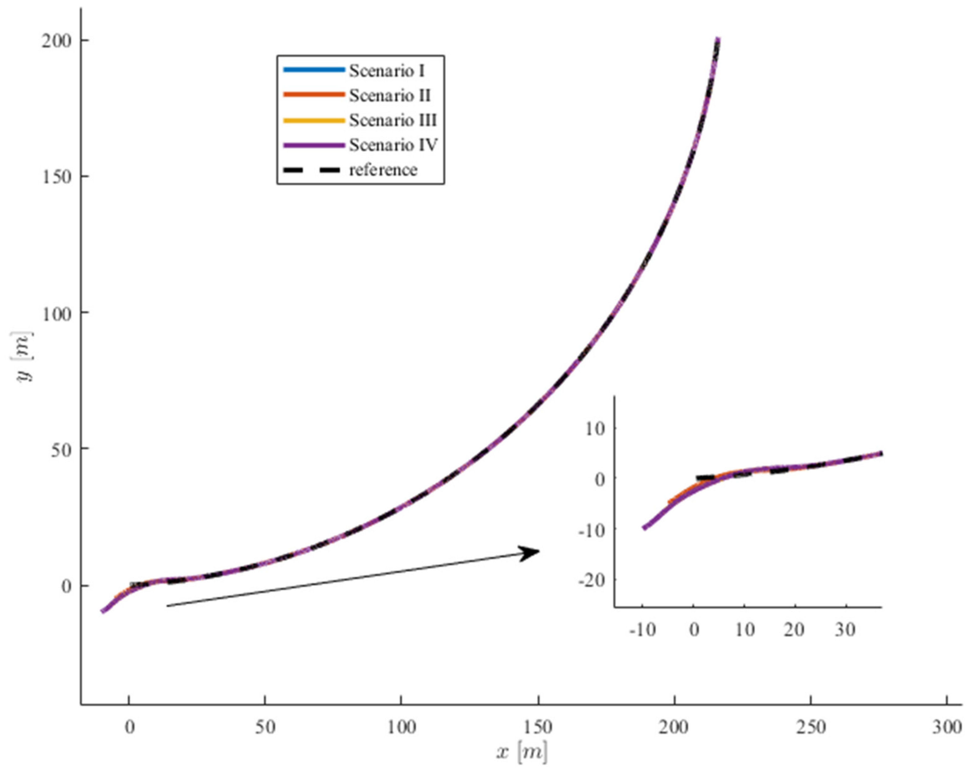
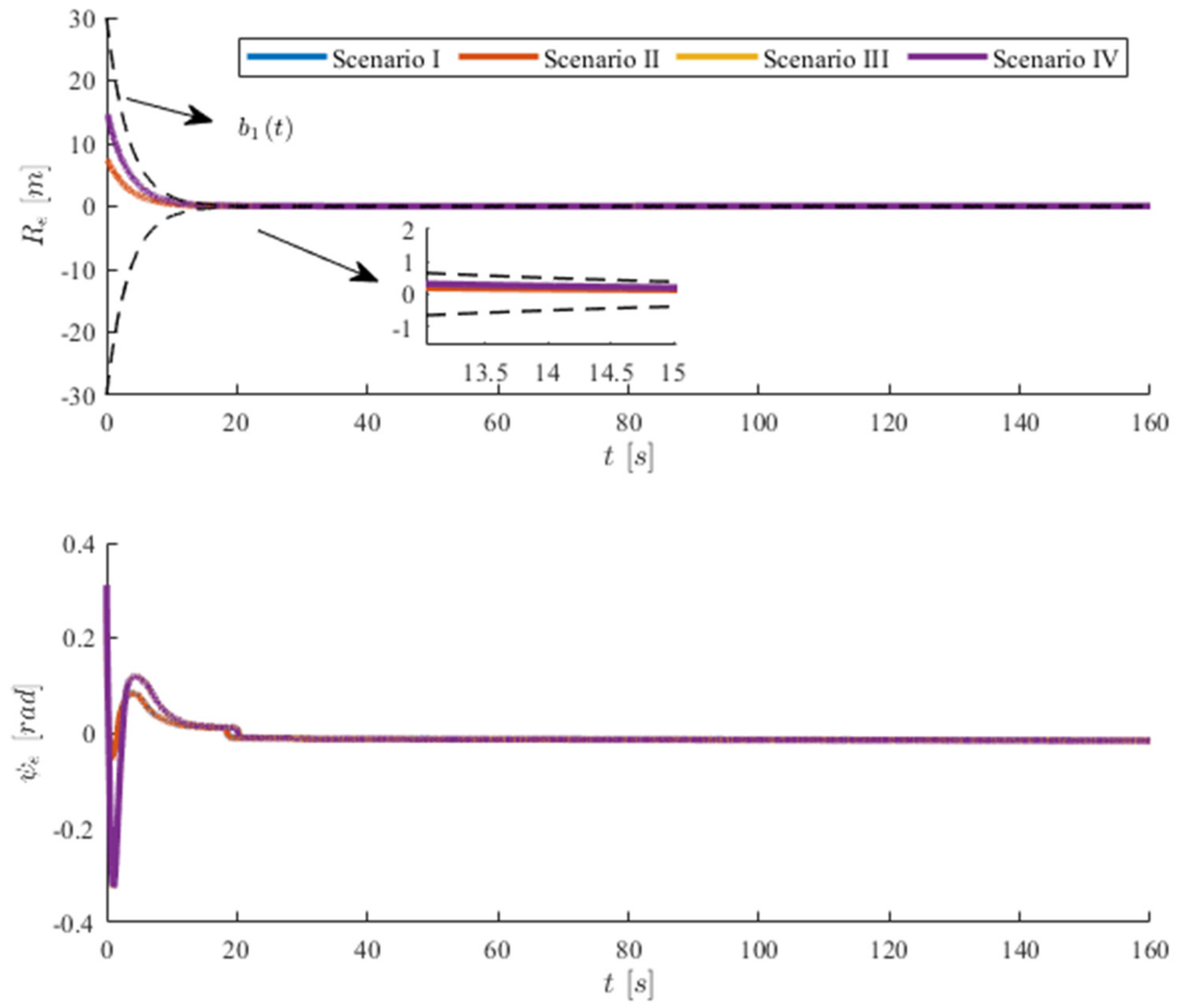
Trajectory tracking in the $x-y$ plane is depicted in Figure 2. Specifically speaking, the position tracking error and the heading tracking error are plotted in Figure 3, respectively. From these results, it is observed that the virtual USV can follow the desired trajectory with a fast convergence speed and satisfactory accuracy. Figure 3 shows that position tracking with a prescribed performance and high stability can be achieved by the proposed controllers. The output constraint of the position is guaranteed with the help of the tangent-type error transformations, thereby meeting the requirements of the science objectives for the given mission.

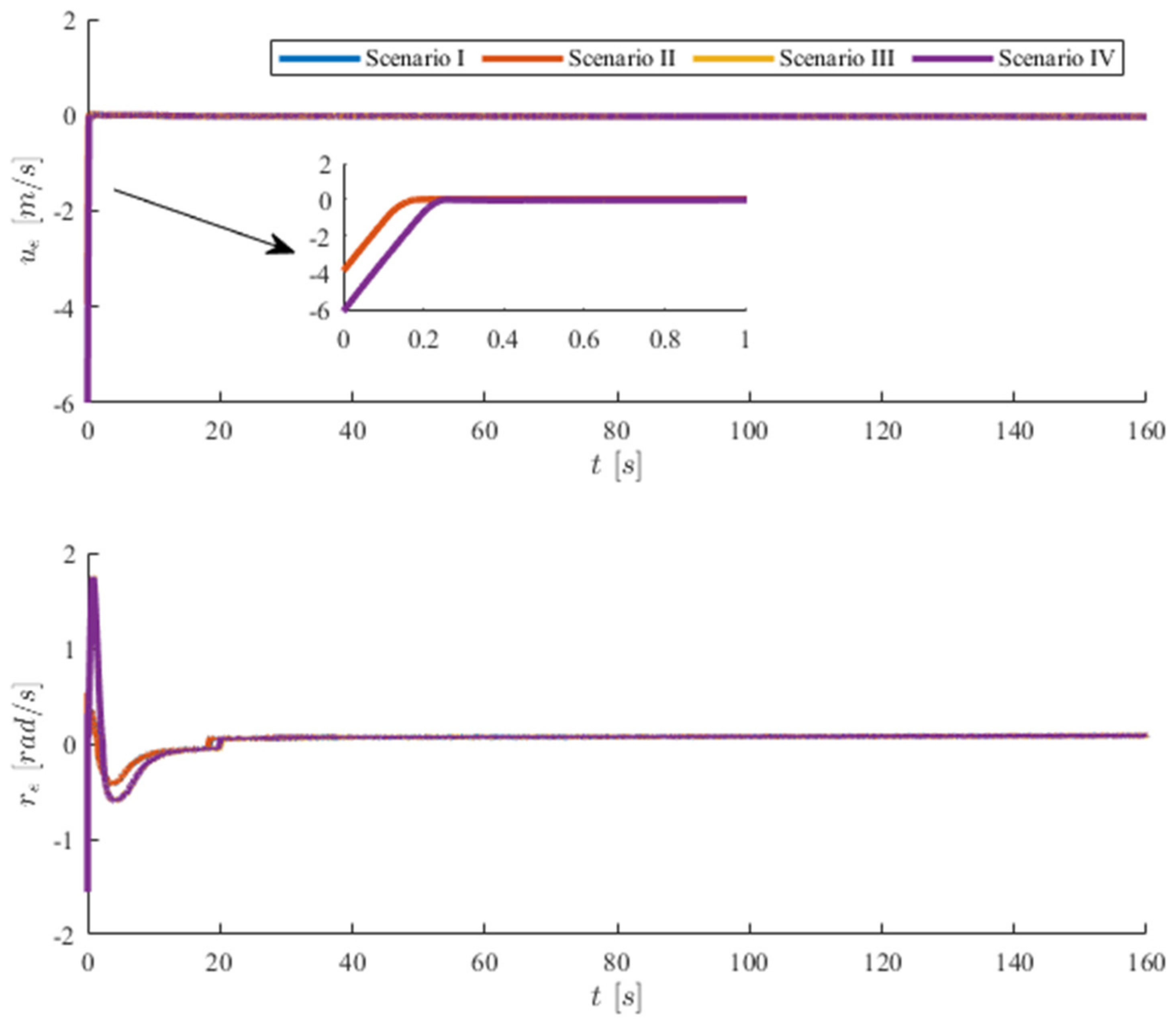
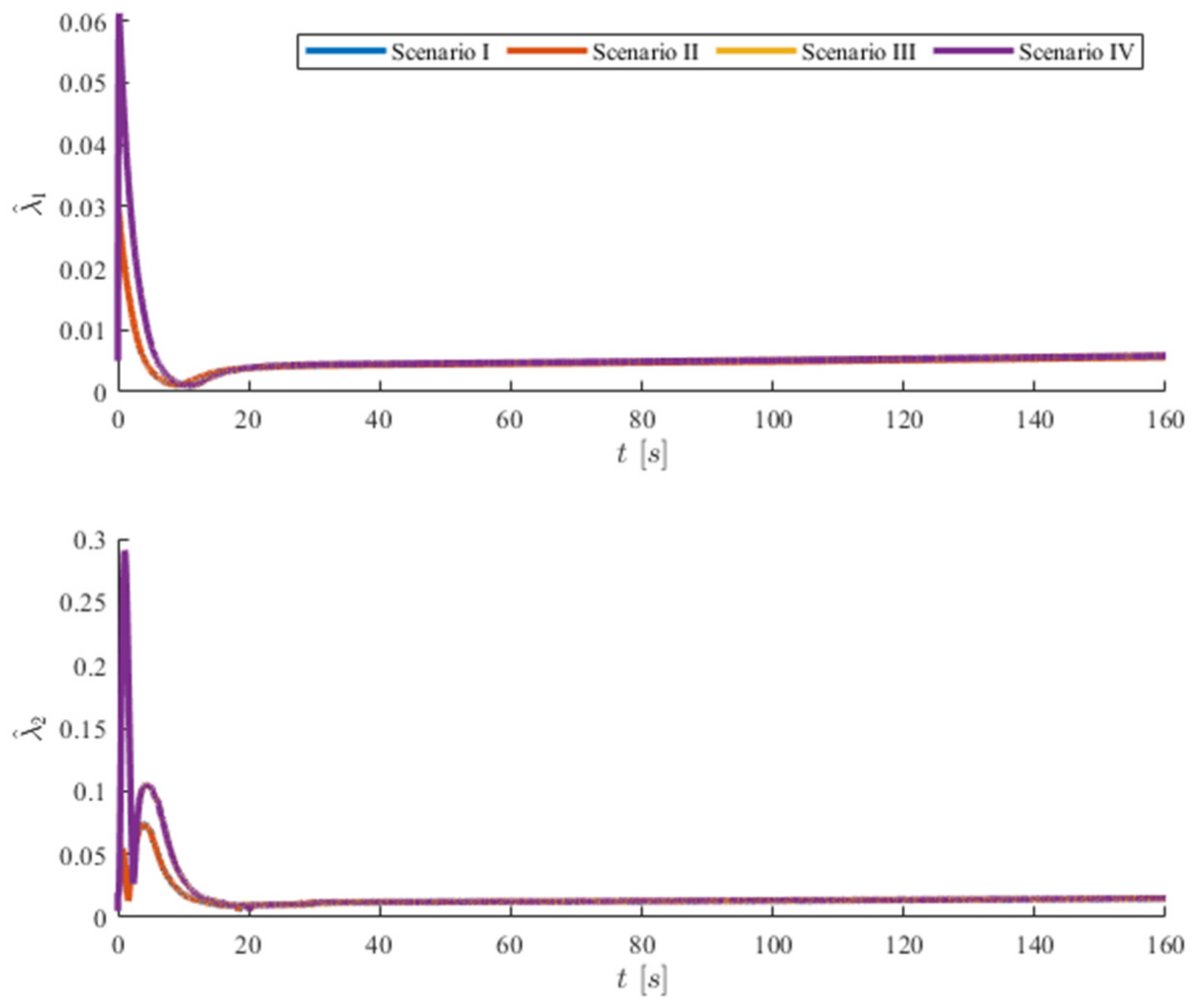
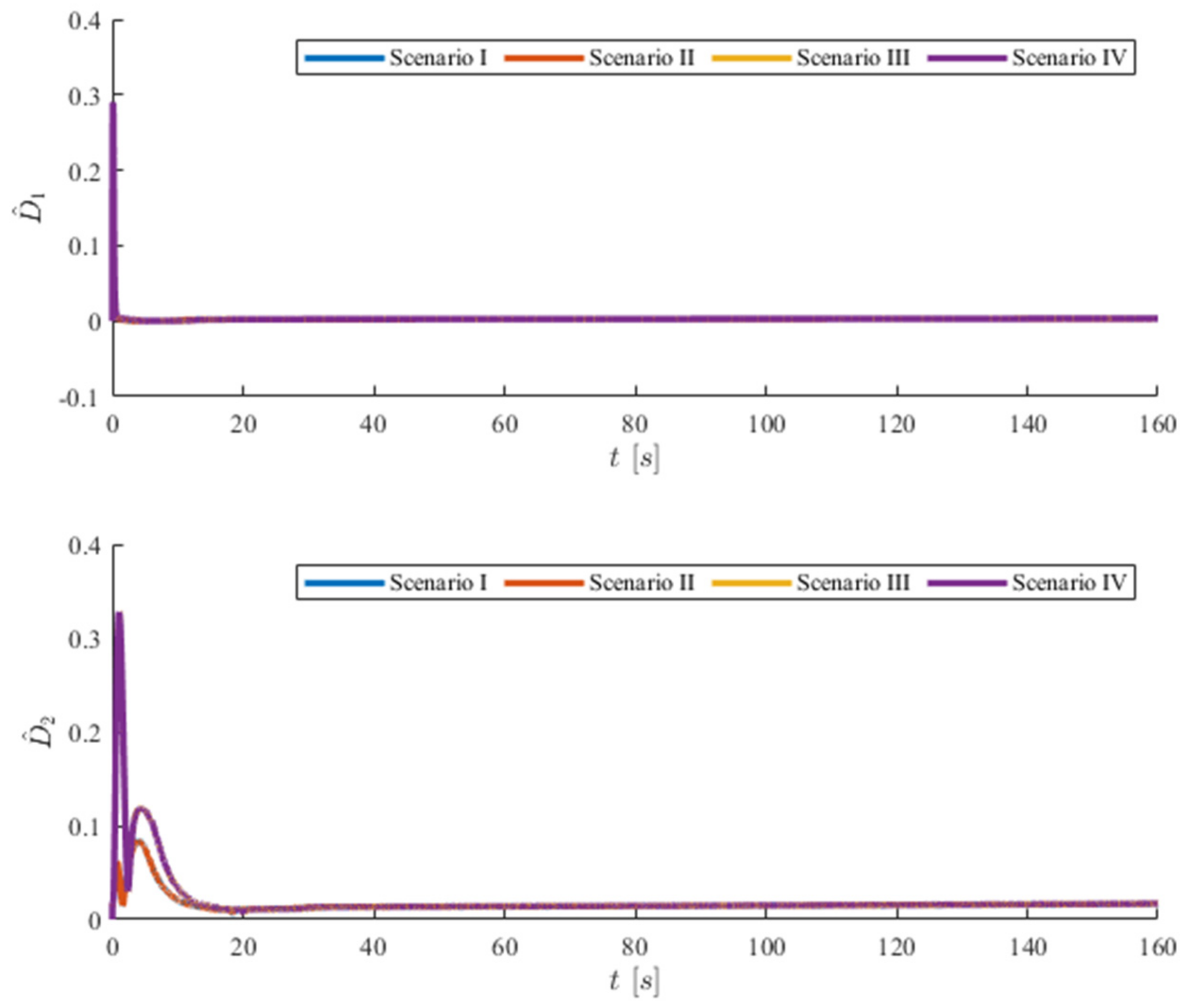
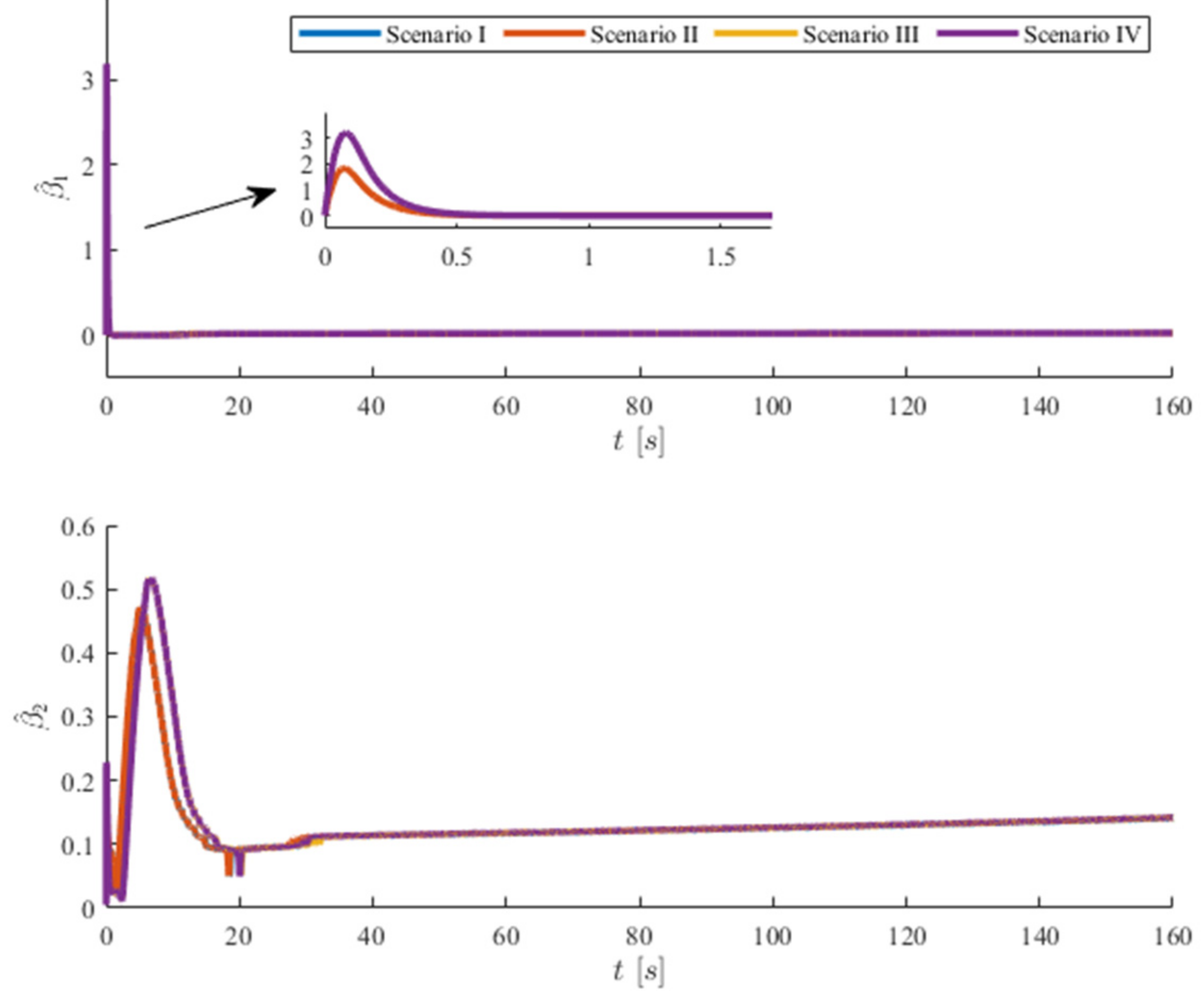
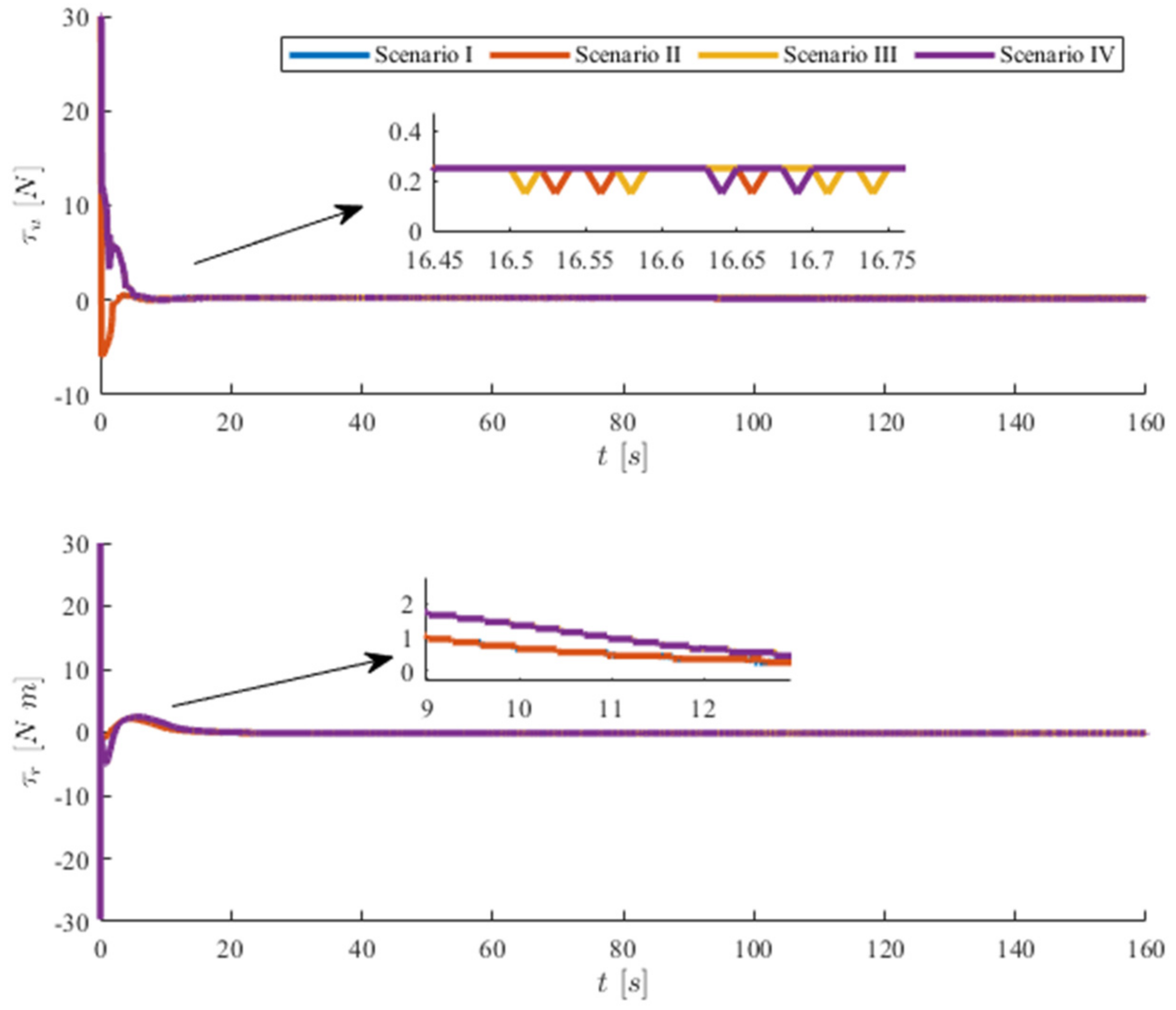
Figure 4 gives the velocity tracking errors of the surge and yaw motions, which can converge to a compact set around the origin quickly and maintain a stable state thereafter. The estimations of the adaptive parameters in surge motion and yaw motion are plotted in Figure 5, Figure 6 and Figure 7. This indicates that all of the adaptive parameters are bounded, which conforms to Theorem 1. Quantized control signals that take values in a finite set are presented in Figure 8. With the consideration of input quantization constraints, it is clear that the control inputs are discrete and keep a constant value within a time interval, meaning that the data transmission will be considerably improved.

From these figures, the boundedness of all of the closed loop signals can be easily verified. That is to say that accurate trajectory tracking and attitude tracking are achieved in this simulation, even in the presence of the quantized inter-vessel transmitted state information, model uncertainties, and external disturbances. Furthermore, by comparing all of the results under different scenarios, the proposed scheme enjoys a high robustness and control performance under different initial tracking errors and disturbances. The above-mentioned simulation analysis is in accordance with Theorem 1.

5. Conclusions

In this paper, a quantized prescribed performance control mechanism that considers uncertain model dynamics and quantizer parameters is proposed for the trajectory tracking of USVs. By combining the adaptive algorithm and the MLP-based NN technique, the global boundedness and asymptotical stability of the closed-loop system are guaranteed. Furthermore, the position tracking error has been constrained to the predefined region with the aid of a tangent-type error transformation. Compared with the exiting quantized framework, the significant advantage of the presented controller is that the information of the HLQ does not need to be accurately known by the designer, while the data transmission burden can be effectively alleviated. Numerical simulations have exhibited the effectiveness and advantages of the control strategy developed.

References

- Zheng, Z.; Ruan, L.; Zhu, M. Output-constrained tracking control of an underactuated autonomous underwater vehicle with uncertainties. Ocean. Eng. 2019, 175, 241–250. [Google Scholar] [CrossRef]
- Zheng, Z.; Huang, Y.; Xie, L.; Zhu, B. Adaptive Trajectory Tracking Control of a Fully Actuated Surface Vessel with Asymmetrically Constrained Input and Output. IEEE Trans. Control. Syst. Technol. 2018, 26, 1851–1859. [Google Scholar] [CrossRef]
- Qin, H.; Li, C.; Sun, Y.; Li, X.; Du, Y.; Deng, Z. Finite-time trajectory tracking control of unmanned surface vessel with error constraints and input saturations. J. Frankl. Inst. 2019, 357, 11472–11495. [Google Scholar] [CrossRef]
- Shen, Z.; Bi, Y.; Wang, Y.; Guo, C. MLP Neural Network-based Recursive Sliding Mode Dynamic Surface Control for Trajectory Tracking of Fully Actuated Surface Vessel Subject to Unknown Dynamics and Input Saturation. Neurocomputing 2020, 377, 103–112. [Google Scholar] [CrossRef]
- Fu, M.; Wang, T.; Wang, C. Adaptive Neural-Based Finite-Time Trajectory Tracking Control for Underactuated Marine Surface Vessels with Position Error Constraint. IEEE Access 2019, 7, 16309–16322. [Google Scholar] [CrossRef]
- Guo, Y.; Huang, B.; Li, A.; Wang, C. Integral sliding mode control for Euler-Lagrange systems with input saturation. Int. J. Robust Nonlinear Control. 2018, 29, 1088–1100. [Google Scholar] [CrossRef]
- Shi, Z.; Deng, C.; Zhang, S.; Xie, Y.; Cui, H.; Hao, Y. Hyperbolic Tangent Function-Based Finite-Time Sliding Mode Control for Spacecraft Rendezvous Maneuver without Chattering. IEEE Access 2020, 8, 60838–60849. [Google Scholar] [CrossRef]
- Zhang, M.; Liu, X.; Yin, B.; Liu, W. Adaptive terminal sliding mode based thruster fault tolerant control for underwater vehicle in time-varying ocean currents. J. Frankl. Inst. 2015, 352, 4935–4961. [Google Scholar] [CrossRef]
- Yu, Y.; Guo, C.; Yu, H. Finite-Time PLOS-Based Integral Sliding-Mode Adaptive Neural Path Following for Unmanned Surface Vessels with Unknown Dynamics and Disturbances. IEEE Trans. Autom. Sci. Eng. 2019, 16, 1500–1511. [Google Scholar] [CrossRef]
- Liao, Y.-L.; Wan, L.; Zhuang, J.-Y. Backstepping Dynamical Sliding Mode Control Method for the Path Following of the Underactuated Surface Vessel. Procedia Eng. 2011, 15, 256–263. [Google Scholar] [CrossRef] [Green Version]
- Wen, G.; Ge, S.S.; Chen, C.L.P.; Tu, F.; Wang, S. Adaptive Tracking Control of Surface Vessel Using Optimized Backstepping Technique. IEEE Trans. Syst. Man Cybern. 2019, 49, 3420–3431. [Google Scholar] [CrossRef]
- Xie, T.; Li, Y.; Jiang, Y.; An, L.; Wu, H. Backstepping active disturbance rejection control for trajectory tracking of underactuated autonomous underwater vehicles with position error constraint. Int. J. Adv. Robot. Syst. 2020, 17, 1729881420909633. [Google Scholar] [CrossRef] [Green Version]
- Zhang, T.; Xia, M.; Zhu, J. Adaptive backstepping neural control of state-delayed nonlinear systems with full-state constraints and unmodeled dynamics. Int. J. Adapt. Control. Signal Process. 2017, 31, 1704–1722. [Google Scholar] [CrossRef]
- Zheng, H.; Wu, J.; Wu, W.; Zhang, Y. Robust dynamic positioning of autonomous surface vessels with tube-based model predictive control. Ocean. Eng. 2020, 199, 106820. [Google Scholar] [CrossRef]
- Zhang, J.; Sun, T.; Liu, Z. Robust model predictive control for path-following of underactuated surface vessels with roll constraints. Ocean. Eng. 2017, 143, 125–132. [Google Scholar] [CrossRef]
- Yu, J.; Shi, P.; Zhao, L. Finite-time command filtered backstepping control for a class of nonlinear systems. Automatica 2018, 92, 173–180. [Google Scholar] [CrossRef]
- Lu, Y.; Zhang, G.; Sun, Z.; Zhang, W. Adaptive cooperative formation control of autonomous surface vessels with uncertain dynamics and external disturbances. Ocean. Eng. 2018, 167, 36–44. [Google Scholar] [CrossRef]
- Xing, L.; Wen, C.; Zhu, Y.; Su, H.; Liu, Z. Output feedback control for uncertain nonlinear systems with input quantization. Automatica 2016, 65, 191–202. [Google Scholar] [CrossRef]
- Xing, L.; Wen, C.; Wang, L.; Liu, Z.; Su, H. Adaptive output feedback regulation for a class of nonlinear systems subject to input and output quantization. J. Frankl. Inst. 2017, 354, 6536–6549. [Google Scholar] [CrossRef]
- Zhou, J.; Wen, C.; Wang, W. Adaptive control of uncertain nonlinear systems with quantized input signal. Automatica 2018, 95, 152–162. [Google Scholar] [CrossRef] [Green Version]
- Zhang, C.H.; Yang, G.H. Event-Triggered Adaptive Output Feedback Control for a Class of Uncertain Nonlinear Systems with Actuator Failures. IEEE Trans. Syst. Man Cybern. 2020, 50, 201–210. [Google Scholar] [CrossRef] [PubMed]
- Wang, A.; Liu, L.; Qiu, J.; Feng, G. Event-Triggered Robust Adaptive Fuzzy Control for a Class of Nonlinear Systems. IEEE Trans. Fuzzy Syst. 2019, 27, 1648–1658. [Google Scholar] [CrossRef]
- Li, T.; Wen, C.; Yang, J.; Li, S.; Guo, L. Event-triggered tracking control for nonlinear systems subject to time-varying external disturbances. Automatica 2020, 119, 109070. [Google Scholar] [CrossRef]
- Wu, B.; Xu, C.; Zhang, Y. Decentralized adaptive control for attitude synchronization of multiple spacecraft via quantized information exchange. Acta Astronaut. 2020, 175, 57–65. [Google Scholar] [CrossRef]
- Liu, R.; Cao, X.; Liu, M.; Zhu, Y. 6-DOF fixed-time adaptive tracking control for spacecraft formation flying with input quantization. Inf. Sci. 2019, 475, 82–99. [Google Scholar] [CrossRef]
- Hu, J.; Sun, X.; Liu, S.; He, L. Adaptive finite-time formation tracking control for multiple nonholonomic UAV system with uncertainties and quantized input. Int. J. Adapt. Control. Signal Process. 2019, 33, 114–129. [Google Scholar] [CrossRef] [Green Version]
- Wang, Y.; He, L.; Huang, C. Adaptive time-varying formation tracking control of unmanned aerial vehicles with quantized input. ISA Trans. 2019, 85, 76–83. [Google Scholar] [CrossRef] [PubMed]
- Yan, Y.; Yu, S. Sliding mode tracking control of autonomous underwater vehicles with the effect of quantization. Ocean. Eng. 2018, 151, 322–328. [Google Scholar] [CrossRef]
- Guo, T.; Wu, X. Backstepping control for output-constrained nonlinear systems based on nonlinear mapping. Neural Comput. Appl. 2014, 25, 1665–1674. [Google Scholar] [CrossRef]
- Jia, Z.; Hu, Z.; Zhang, W. Adaptive output-feedback control with prescribed performance for trajectory tracking of underactuated surface vessels. ISA Trans. 2019, 95, 18–26. [Google Scholar] [CrossRef] [PubMed]
- Dai, S.-L.; He, S.; Wang, M.; Yuan, C. Adaptive Neural Control of Underactuated Surface Vessels with Prescribed Performance Guarantees. IEEE Trans. Neural Netw. 2019, 30, 3686–3698. [Google Scholar] [CrossRef]
- Park, B.S.; Yoo, S.J. Robust fault–tolerant tracking with predefined performance for underactuated surface vessels. Ocean. Eng. 2016, 115, 159–167. [Google Scholar] [CrossRef]
- He, W.; Yin, Z.; Sun, C. Adaptive Neural Network Control of a Marine Vessel with Constraints Using the Asymmetric Barrier Lyapunov Function. IEEE Trans Cybern. 2017, 47, 1641–1651. [Google Scholar] [CrossRef] [PubMed]
- Jin, X. Fault tolerant finite-time leader–follower formation control for autonomous surface vessels with LOS range and angle constraints. Automatica 2016, 68, 228–236. [Google Scholar] [CrossRef]
- Shao, X.; Shi, Y. Neural adaptive control for MEMS gyroscope with full-state constraints and quantized input. IEEE Trans. Ind. Inform. 2020, 16, 6444–6454. [Google Scholar] [CrossRef]
- Chen, Z.; Zhang, Y.; Zhang, Y.; Nie, Y.; Tang, J.; Zhu, S. Disturbance-Observer-Based Sliding Mode Control Design for Nonlinear Unmanned Surface Vessel with Uncertainties. IEEE Access 2019, 7, 148522–148530. [Google Scholar] [CrossRef]
- An, H.; Wu, Q.; Wang, G.; Guo, Z.; Wang, C. Simplified longitudinal control of air-breathing hypersonic vehicles with hybrid actuators. Aerosp. Sci. Technol. 2020, 104, 105936. [Google Scholar] [CrossRef]
Figure 1.
Structure of the trajectory tracking control system of USV.
Figure 2.
Trajectories of the USV in the 2D plane.
Figure 3.
Time responses of position tracking errors and heading tracking errors.
Figure 4.
Time responses of velocity tracking errors.
Figure 5.
Time responses of adaptive parameter estimations and .
Figure 6.
Figure 7.
Figure 8.
Time responses of quantized control forces.