Stability Analysis of a Diffusive Three-Species Ecological System with Time Delays

Abstract

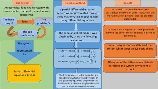
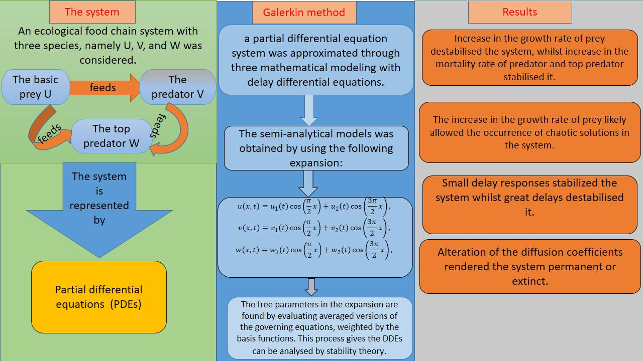
In this study, the dynamics of a diffusive Lotka–Volterra three-species system with delays were explored. By employing the Galerkin Method, which generates semi-analytical solutions, a partial differential equation system was approximated through mathematical modeling with delay differential equations. Steady-state curves and Hopf bifurcation maps were created and discussed in detail. The effects of the growth rate of prey and the mortality rate of the predator and top predator on the system’s stability were demonstrated. Increase in the growth rate of prey destabilised the system, whilst increase in the mortality rate of predator and top predator stabilised it. The increase in the growth rate of prey likely allowed the occurrence of chaotic solutions in the system. Additionally, the effects of hunting and maturation delays of the species were examined. Small delay responses stabilised the system, whilst great delays destabilised it. Moreover, the effects of the diffusion coefficients of the species were investigated. Alteration of the diffusion coefficients rendered the system permanent or extinct.

1. Introduction

Recently, the population dynamics of various biological and ecological systems have garnered much attention, promoting the emergence of mathematical models describing population dynamics and species interactions. These mathematical models must incorporate both spatial diffusion and time delays to mirror the dynamic nature of biological systems and the tendency of the species to move to the least densely populated areas. Reaction–diffusion models with time delays, which show oscillatory phenomena, can describe the delayed response to past conduct and the spatial structure of chemical, biological, and ecological systems [1,2,3,4]. In particular, the delay-diffusive logistic equation describes the growth dynamics of a single species, whilst the delay-diffusive Lotka–Volterra predator-prey model describes the dynamics of multiple species [5,6,7].

In recent years, the predator-prey relationship represents the most studied of environmental dynamics. In the 1920s, Alfred Lotka and Vito Volterra [8] proposed a mathematical model for a predator-prey system, which described the fish catch in the Atlantic. This model can also be utilised to study physical systems and chemical reactions, such as the dynamics of resonantly coupled lasers [8,9]. Several studies have examined the stability of the Lotka–Volterra predator-prey model. For instance, Faria [10] investigated the predator-prey system with one or two time delays and a unique positive equilibrium. They examined the dynamics of this system based on the local stability of the equilibrium and the region of the Hopf bifurcation map that has been proven to occur when one of the delays is assumed to be a bifurcation parameter. Yan and Chu [11] explored the stability of the Lotka–Volterra predator-prey model and found conditions for the occurrence of oscillating solutions. The authors also studied the stability of the oscillating solutions. Chen et al. [12] analysed the diffusive Lotka–Volterra predator–prey model with two delays. The authors explored the stability of Hopf bifurcations and the equilibrium of coexistence by analysing the characteristic equations and found that through a Hopf bifurcation, the positive equilibrium point of the system could be destabilised with an increase in the magnitude of delay. Tahara et al. [13] studied the dynamics of Lotka–Volterra systems and showed that the predator–prey populations could be stabilised by including small immigration into the prey or predator population. Al Noufaey [14] considered a diffusive Lotka–Volterra predator–prey system with multiple delays in one and two-dimensional domains. The authors obtained simple approximate linear expressions describing the steady-state solutions and the Hopf bifurcation regions and also found that the delays either stabilise or destabilise the system. Shenghu [15] analysed the stability of a diffusive Lotka–Volterra system with a prey-stage structure. The author demonstrated the effects of high diffusion rates on the presence of positive steady states. A high diffusion rate of the prey species could destroy the spatial pattern, whereas a high diffusion rate of the predator species could conserve the spatial pattern.

Meanwhile, the food webs and food chains, including three or more species, comprise all components for the occurrence of chaos. This has encouraged several researchers to study the chaotic dynamics of an ecosystem [5,16,17,18,19,20]. Naji and Balasim [21] considered a three-species food chain with the Beddington–DeAngelis response and obtained different stability conditions of the system. The authors also illustrated diverse chaotic behaviours in the system under realistic feasible parameter values. Pao [22] studied a three species time-delayed Lotka–Volterra reaction–diffusion system and obtained certain conditions of the existence and global asymptotic stability of a positive steady-state solution. They also showed that the three-species could coexist and that all trivial and semi-trivial solutions were unstable. Liao [23] investigated a competitive Lotka–Volterra system with three delays without diffusion and found that the system was destabilised when the delay parameter exceeded the critical value. In the real world, the applications of three-species systems have been studied widely [24,25]. Example of these applications include the study of crops as prey, aphids as a predator, and lady beetles as a top predator [26].

Semi-analytical solutions based on the Galerkin method [27] were highly efficient and extremely accurate in terms of describing a reaction–diffusion system represented by partial differential equations (PDEs). Marchant [28] applied the Galerkin method to the Gray Scott model. Accordingly, mathematical models based on PDEs could be formulated through the simplest approximations of a system of ordinary differential equations (ODEs). Subsequently, the author used the combustion theory to analyse the stability of the model and observed a great match between the numerical results of the PDEs and the semi-analytical method. Furthermore, many studies have proven the efficiency of this method in analysing the dynamics of chemical reactions and biological systems [28,29,30,31,32,33,34,35,36,37,38,39,40,41].

In reality, population dynamic issues are tied to both space and time, which implies that the state change will be impacted by both the present state and also the past. To this end, the present study aimed to analyse a three-species predator-prey Lotka–Volterra reaction–diffusion model by taking the effects of both diffusion and time delay into account. The organisation of this research article is as follows. Section 2 presents the diffusive Lotka–Volterra three-species system with delays and describes the semi-analytical solutions obtained using the Galerkin method based on the PDE system approximated through mathematical modeling with delay differential equations (DDEs). Section 3 describes steady-state analyses and profiles. Section 4 discusses the methods for determining the stability and Hopf bifurcation points of the DDE system and presents the Hopf bifurcation maps and limit cycles. Section 5 presents bifurcation diagrams showing the occurrence of chaos in the system. The final section presents concluding remarks.

2. Mathematical Model and Methods

2.1. Mathematical Model

An ecological food chain with three species, namely U, V, and W was considered. U indicates the basic prey, V indicates the predator which consumes U, and W is the top predator which consumes both U and V. Through the Lotka–Volterra type of interactions and the effects of diffusion and time delays for each species, this system can be modelled by the following delay reaction–diffusion equations:

$$\begin{array}{ccc}& & u_t=D_1{u}_{xx}+u(\alpha -{\delta }_{1}u-{\mu }_{1}v(t-{\tau }_1)-{\kappa }_{1}w(t-{\tau }_2)),\hfill \\ & & v_t=D_2{v}_{xx}+v(-\beta +{\delta }_{2}u(t-{\tau }_3)-{\mu }_{2}v-{\kappa }_{2}w(t-{\tau }_2)),\hfill \\ & & w_t=D_3{w}_{xx}+w(-\gamma +{\delta }_{3}u(t-{\tau }_3)+{\mu }_{3}v(t-{\tau }_1)-{\kappa }_{3}w),\hfill \end{array}$$

(1)

$$\begin{array}{ccc}& & u_x=v_x=w_x=0\mathrm{at}x=0\mathrm{and}u=vs.=w=0\mathrm{at}x=\pm 1\hfill \\ & & u=u_{\varphi }\mathrm{at}-{\tau }_3<t\le 0,vs.=v_{\varphi }\mathrm{at}-{\tau }_1<t\le 0,\hfill \\ & & \mathrm{and}w=w_{\varphi }\mathrm{at}-{\tau }_2<t\le 0.\hfill \end{array}$$

(2)

In the equations above, u, v, and w are the corresponding scaled concentrations of the population densities of the prey, predator, and top predator, respectively. At $x=0$, zero-flux boundary conditions are applied; thus, it is an impermeable boundary as it indicates that there is no population flux across the boundary. At $x=\pm 1$, the Dirichlet boundary conditions are applied, which indicate that the population is fixed [14,42]. So the solution is symmetric about the center of the domain $x=0$. Thus, system (1) and (2) is open and allows for the occurrence of steady-state solutions, periodic oscillations, and chaotic behaviours. Here, the intrinsic growth rate of the prey species is denoted by the parameter $\alpha$, whilst the mortality rates of the predator and top predator species are represented by the parameters $\beta$ and $\gamma$, respectively. The carrying capacities of the populations of the three species, namely the prey u, predator v, and top predator w, are represented by the parameters ${\delta }_1$, ${\mu }_2$, and ${\kappa }_3$, respectively. ${\mu }_1$ and ${\kappa }_1$ indicate the reduction in the prey population as a result of the presence of the predator and top predator, respectively. ${\delta }_2$ indicates the increase in the predator population as a result of the presence of prey, whilst ${\kappa }_2$ represents the decrease in the predator population as a result of the presence of the top predator. The parameters ${\delta }_3$ and ${\mu }_3$ indicate the increase in the top predator population as a result of the presence of the prey and predator, respectively. ${\tau }_i$$(i=1\dots 3)$ refers to hunting and maturation delays. The parameters $D_i$$(i=1\dots 3)$ indicate the diffusion coefficients of the three species u, v, and w. For physically realistic population models, all parameters are positive. On the other hand, if the top predator population (w) is zero, (where $D_3=\gamma ={\mu }_3={\kappa }_i=0$; $i=1\dots 3$), then the system (1) reduces to the two-species prey–predator model, which has been investigated in [14].

2.2. Galerkin Method

By applying the Galerkin method, the semi-analytical model (1) was obtained and developed in a one dimensional $(1-D)$ spatial domain. This method is based on the approximation of the spatial structure of the population density profile using a set of basis functions, converting the governing PDE (1) and boundary conditions (2) for formulation with the simplest possible laws of the fundamental equations of the DDE system. Here, we use the expansion function to represent the two-term semi-analytical method as follows:

$$\begin{array}{ccc}\hfill u(x,t)& =& u_1\left(t\right)cos\left(\frac{\pi x}{2}\right)+u_2\left(t\right)cos\left(\frac{3\pi x}{2}\right),\hfill \\ \hfill v(x,t)& =& v_1\left(t\right)cos\left(\frac{\pi x}{2}\right)+v_2\left(t\right)cos\left(\frac{3\pi x}{2}\right),\hfill \\ \hfill w(x,t)& =& w_1\left(t\right)cos\left(\frac{\pi x}{2}\right)+w_2\left(t\right)cos\left(\frac{3\pi x}{2}\right).\hfill \end{array}$$

(3)

This expansion function (3) fulfills the given boundary conditions (2) and also has the property that the concentrations of the population densities at the impermeable boundary $x=0$ are $u=\Sigma u_i$, $v=\Sigma v_i$ and $w=\Sigma w_i$, $i=1,2$. The averaged versions of the governing PDEs, weighted using the basis functions, must be evaluated to find the free parameters that exist in (3). This technique yields the DDEs, see (A1) in the Appendix A.

The DDEs (A1) are obtained by truncating series (3) using a two-term combination. The use of the two-term method is preferred due to its accuracy without the need to lengthen the expression [14,28]. Moreover, the one-term solution (when $u_2=v_2=w_2=0$) was calculated to ensure accuracy in comparison.

The numerical simulation results of the DDEs (A1) is obtained using a fourth-order Runge–Kutta method, while the numerical solutions of the PDEs model (1) and (2) are found using a Crank–Nicholson finite-difference scheme. The percentage error, which is the absolute value of the difference between the approximate (one- or two- terms) and exact (numerical of PDEs) values divided by the exact value multiplied by 100, is used to calculate the difference between the one- and two-term solutions and the numerical solution of (1) and (2).

3. Positive Steady-State Analysis and Profiles

This section discusses the steady-state solutions of the system. All time derivative terms in (A1) are zero at the steady-state, yielding a set of six transcendental equations. Additionally, we let $u_i\left(t\right)=u_i(t-{\tau }_3)=u_{is}$, $v_i\left(t\right)=v_i(t-{\tau }_1)=v_{is}$, and $w_i\left(t\right)=w_i(t-{\tau }_2)=w_{is}$, $i=1,2$ and inserted these terms back into the Equation (A1). As a result, we obtained six transcendental equations, $f_i=0,i=1,\dots ,6$, which can be solved numerically and also make use of (3). For the one-term semi-analytical model case ($u_{is}=v_{is}=w_{is}=0$), we obtained three transcendental equations. The system yielded five non-negative steady-state solutions ($s{s}_i$). For the one-term semi-analytical model, the steady-state solutions at the origin steady-state point $s{s}_1=(u_1,v_1,w_1)=(0,0,0)$ always exist and the axial steady-state point $s{s}_2=(\frac{3\pi (4\alpha -D_1{\pi }^2)}{32{\delta }_1},0,0)$ exists only if $\alpha >\frac{D_1{\pi }^2}{4}$; the two boundary steady-state points $s{s}_3=(\frac{3\pi (D_3{\pi }^2{\kappa }_1+4\gamma {\kappa }_1+4\alpha {\kappa }_3-D_1{\pi }^2{\kappa }_3)}{32({\delta }_1{\kappa }_3+{\delta }_3{\kappa }_1)},0,\frac{3\pi (4\alpha {\delta }_3-D_1{\pi }^2{\delta }_3-D_3{\pi }^2{\delta }_1-4\gamma {\delta }_1)}{32({\delta }_1{\kappa }_3+{\delta }_3{\kappa }_1)})$ and $s{s}_4=(\frac{3\pi (D_2{\pi }^2{\mu }_1+4\beta {\mu }_1+4\alpha {\mu }_2-D_1{\pi }^2{\mu }_2)}{32({\delta }_1{\mu }_2+{\delta }_2{\mu }_1)},\frac{3\pi (4\alpha {\delta }_2-D_1{\pi }^2{\delta }_2-D_2{\pi }^2{\delta }_1-4\beta {\delta }_1)}{32({\delta }_1{\mu }_2+{\delta }_2{\mu }_1)},0)$ and one interior steady-state point $s{s}_5=(u_1^{*},v_1^{*},w_1^{*})$ are given by:

$$\begin{array}{c}\hfill u_1^{*}=\frac{-3\pi (D_1{\pi }^2{\kappa }_2{\mu }_3+D_1{\pi }^2{\kappa }_3{\mu }_2-D_2{\pi }^2{\kappa }_1{\mu }_3-D_2{\pi }^2{\kappa }_3{\mu }_1-D_3{\pi }^2{\kappa }_1{\mu }_2)}{32({\delta }_1{\kappa }_2{\mu }_3+{\delta }_1{\kappa }_3{\mu }_2+{\delta }_2{\kappa }_1{\mu }_3+{\delta }_2{\kappa }_3{\mu }_1+{\delta }_3{\kappa }_1{\mu }_2-{\delta }_3{\kappa }_2{\mu }_1)}\\ \hfill -\frac{3\pi (D_3{\pi }^2{\kappa }_2{\mu }_1-4(\gamma {\kappa }_1{\mu }_2+\gamma {\kappa }_2{\mu }_1-\beta {\kappa }_1{\mu }_3-\beta {\kappa }_3{\mu }_1-\alpha {\kappa }_2{\mu }_3-\alpha {\kappa }_3{\mu }_2))}{32({\delta }_1{\kappa }_2{\mu }_3+{\delta }_1{\kappa }_3{\mu }_2+{\delta }_2{\kappa }_1{\mu }_3+{\delta }_2{\kappa }_3{\mu }_1+{\delta }_3{\kappa }_1{\mu }_2-{\delta }_3{\kappa }_2{\mu }_1)},\\ \hfill v_1^{*}=\frac{-3\pi (D_1{\pi }^2{\delta }_2{\kappa }_3-D_1{\pi }^2{\delta }_3{\kappa }_2+D_2{\pi }^2{\delta }_1{\kappa }_3+D_2{\pi }^2{\delta }_3{\kappa }_1-D_3{\pi }^2{\delta }_1{\kappa }_2)}{32({\delta }_1{\kappa }_2{\mu }_3+{\delta }_1{\kappa }_3{\mu }_2+{\delta }_2{\kappa }_1{\mu }_3+{\delta }_2{\kappa }_3{\mu }_1+{\delta }_3{\kappa }_1{\mu }_2-{\delta }_3{\kappa }_2{\mu }_1)}\\ \hfill -\frac{3\pi (-D_3{\pi }^2{\delta }_2{\kappa }_1-4\gamma {\delta }_1{\kappa }_2+4(\gamma {\delta }_2{\kappa }_1+\beta {\delta }_1{\kappa }_3+\beta {\delta }_3{\kappa }_1-\alpha {\delta }_2{\kappa }_3+\alpha {\delta }_3{\kappa }_2))}{32({\delta }_1{\kappa }_2{\mu }_3+{\delta }_1{\kappa }_3{\mu }_2+{\delta }_2{\kappa }_1{\mu }_3+{\delta }_2{\kappa }_3{\mu }_1+{\delta }_3{\kappa }_1{\mu }_2-{\delta }_3{\kappa }_2{\mu }_1)},\\ \hfill w_1^{*}=-\frac{3\pi (D_1{\pi }^2{\delta }_2{\mu }_3+D_1{\pi }^2{\delta }_3{\mu }_2+D_2{\pi }^2{\delta }_1{\mu }_3-D_2{\pi }^2{\delta }_3{\mu }_1+D_3{\pi }^2{\delta }_1{\mu }_2}{32({\delta }_1{\kappa }_2{\mu }_3+{\delta }_1{\kappa }_3{\mu }_2+{\delta }_2{\kappa }_1{\mu }_3+{\delta }_2{\kappa }_3{\mu }_1+3{\delta }_3{\kappa }_1{\mu }_2-{\delta }_3{\kappa }_2{\mu }_1)}\\ \hfill -\frac{3\pi (D_3{\pi }^2{\delta }_2{\mu }_1+4(\gamma {\delta }_1{\mu }_2+\gamma {\delta }_2{\mu }_1+\beta {\delta }_1{\mu }_3-\beta {\delta }_3{\mu }_1-\alpha {\delta }_2{\mu }_3-\alpha {\delta }_3{\mu }_2))}{32({\delta }_1{\kappa }_2{\mu }_3+{\delta }_1{\kappa }_3{\mu }_2+{\delta }_2{\kappa }_1{\mu }_3+{\delta }_2{\kappa }_3{\mu }_1+3{\delta }_3{\kappa }_1{\mu }_2-{\delta }_3{\kappa }_2{\mu }_1)}.\end{array}$$

(4)

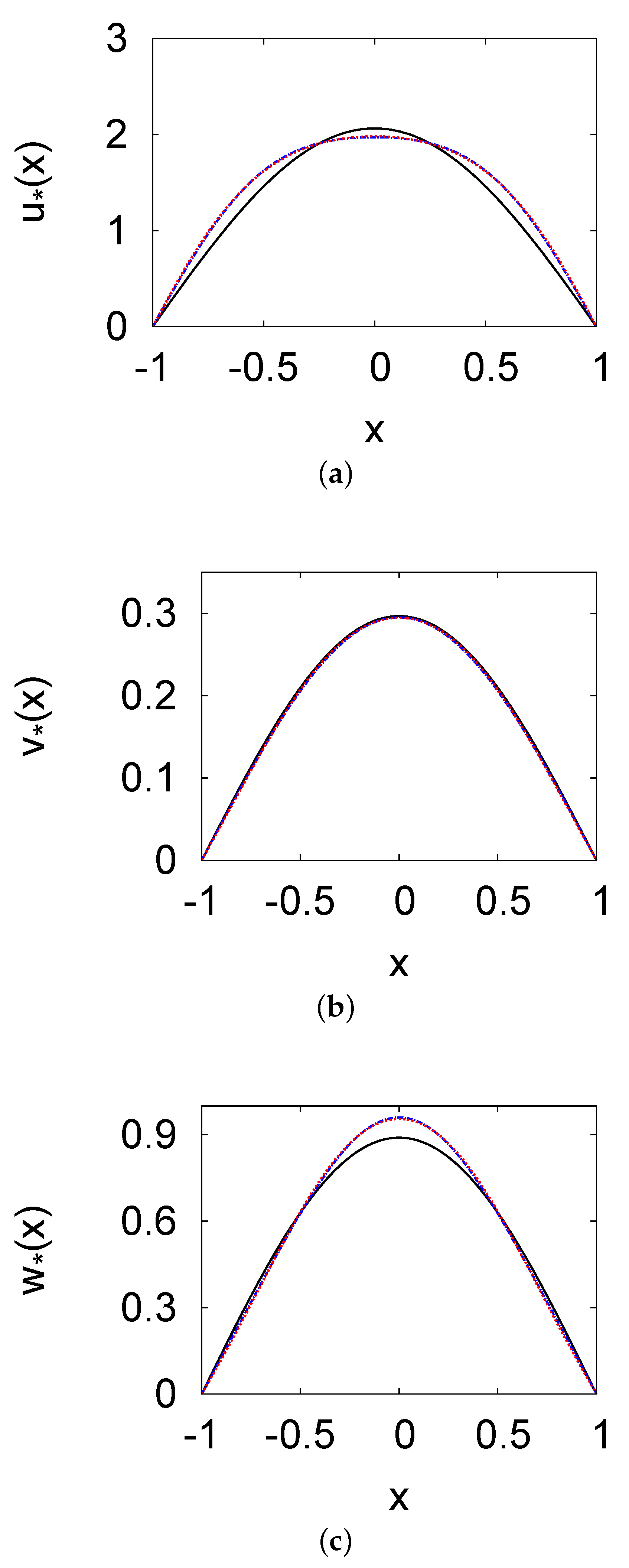
In Figure 1a–c, the steady-state population density profiles of the prey u, the predator v, and the top predator w versus x are shown, respectively. These profiles illustrate the numerical solution of systems (1) and (2) and the solutions of the one and two terms method with the parameters $\alpha =0.5$, $\beta =0.1$, $\gamma =0.4$, $D_1=D_2=D_3=0.05$, ${\mu }_1={\delta }_3={\kappa }_3=0.5$, ${\mu }_2={\delta }_2={\kappa }_2=0.3$, and ${\mu }_3={\delta }_1={\kappa }_1=0.1$. The prey, predator, and top predator densities are highest at the domain centre, where all species migrate across the domain boundaries to maintain a constant population density at zero. The population density peaks are $(u,v,w)=(2.063,0.297,0.890)$ (for the one-term method), $(u,v,w)=(1.971,0.295,0.960)$ (for the two-term method), and $(u,v,w)=(1.982,0.295,0.955)$ (for the numerical solution) at $x=0$. Compared with the numerical solution of PDEs (1), the two-term method yielded an excellent approximation. For the prey, predator, and top predator population density, the errors were <0.6%. The errors were marginally higher for the one-term method, but did not exceed $7\%$. The two-term method was superior to the one-term profile, because it more effectively modelled flat u, v, and w population density profiles.

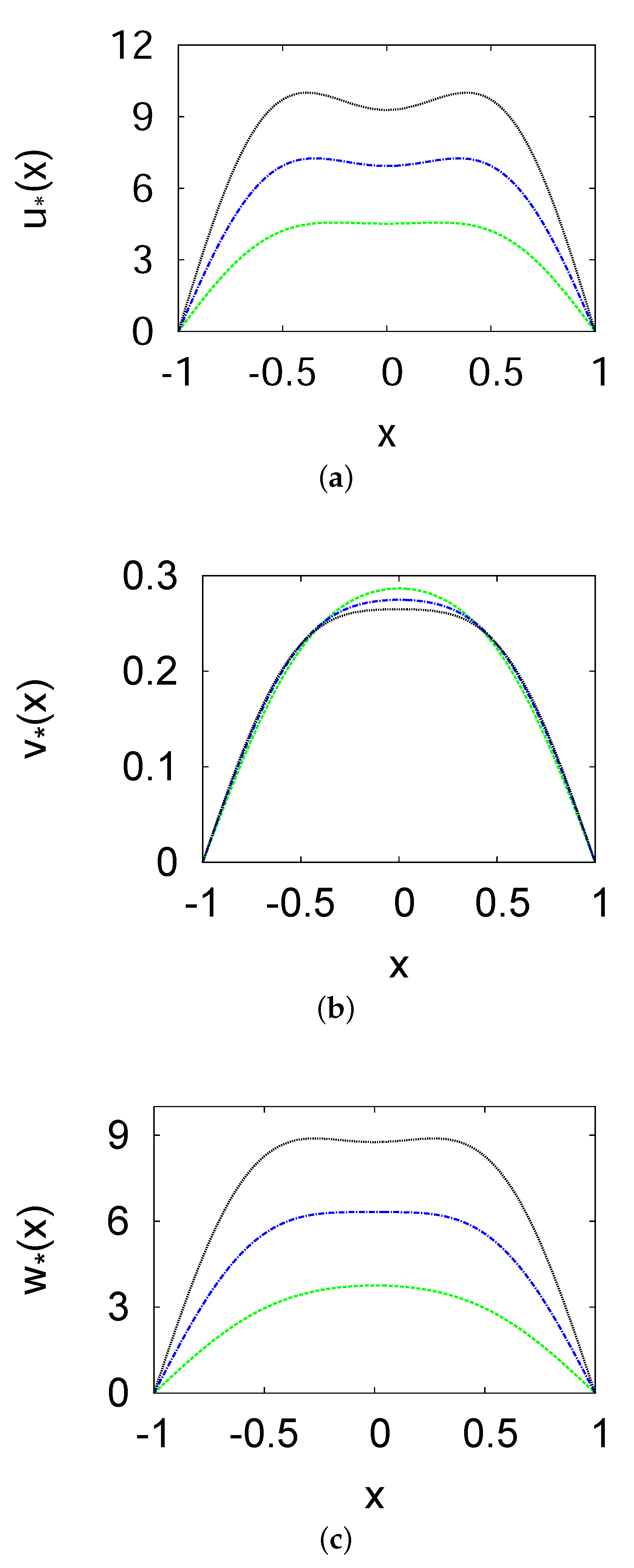
In Figure 2, the effects of different growth rates ($\alpha$) of the prey on the population density profiles of the species are presented. The figure shows the results of the two-term method at different values of $\alpha$ (1, $1.5$, and 2); the other parameters are the same as those in Figure 1. These results suggest that an increase in the prey growth rate $\alpha$ is consistent with increase in the population density of the prey u and top predator w and decrease in the population density of the predator v. In other words, the top predator consumes the predator. At $x=0$, the peaks of the population density of the species reach the following values: $(u,v,w)=(4.517,0.287,3.757)$ when $\alpha =1$, $(u,v,w)=(6.933,0.275,6.320)$ when $\alpha =1.5$, and $(u,v,w)=(9.280,0.265,8.761)$ when $\alpha =2$. Furthermore, as the growth rate of prey increases, the population density of prey migrates from the center and moves to the boundary of the domain.

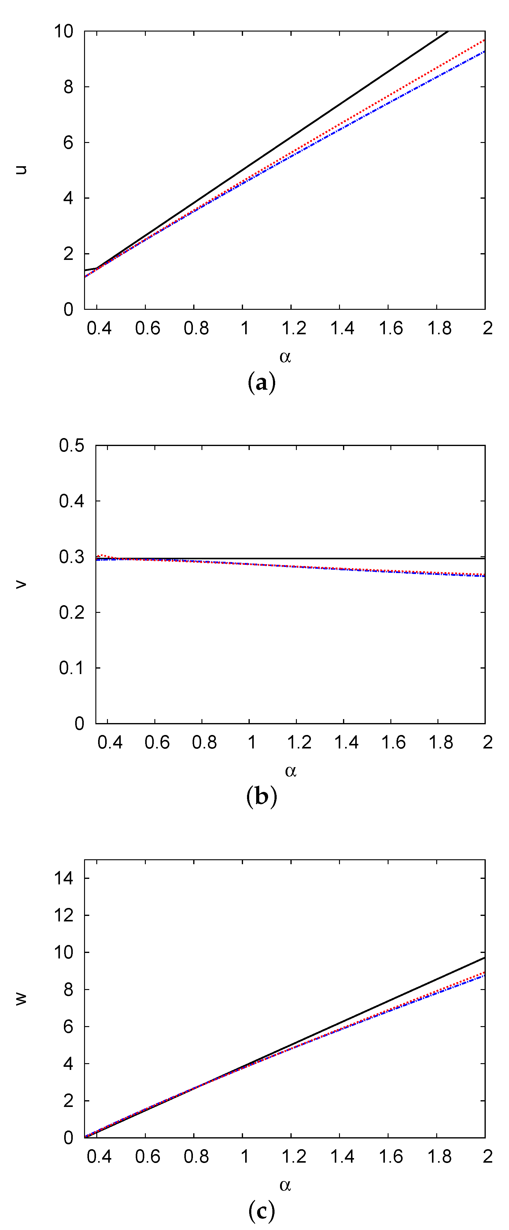
Figure 3 presents the steady-state population densities of the species u, v, and w versus the prey growth rate $\alpha$. It demonstrates the solutions of both the one- and two-term methods, as well as the numerical solution with a group of other feasible parameter values shown in Figure 1. As $\alpha$ increases, the steady-state population densities of the prey u and top predator w increase linearly whereas the steady-state population density of the predator v decreases. The steady-state solutions of the two-term method can be calculated as $u=5.439\alpha -0.74$, $v=0.014\alpha -0.289$, and $w=6.1163\alpha -2.087$. The solution for w turns positive at $\alpha =0.35$, indicating that physically feasible solutions exist at $\alpha \ge 0.35$. The figure shows a significant concordance between the results of the two-term method and the numerical solutions of the PDEs, with an error of <2.6%. At $\alpha =1.2$, the solutions of the one- and two-term methods are $(u,v,w)=(6.187,0.297,5.013)$ and $(u,v,w)=(5.495,0.283,4.802)$, respectively, whilst the numerical solutions of the PDEs are $(u,v,w)=(5.639,0.282,4.812)$.

4. Hopf Bifurcations and Stability Analysis

4.1. Theoretical Framework

This section explains the methods for determining the stability and Hopf bifurcation points of the DDEs system (A1). A common phenomenon in biological, chemical, and physical models is Hopf bifurcation, which arises when periodic solutions occur through a local change in the stability of a steady state as a result of crossing a conjugated pair of eigenvalues over an imaginary axis. The standard literature on bifurcation theory and dynamical systems [43,44,45,46] has clarified the Hopf bifurcation theory. Moreover, many researchers discussed the techniques to find the Jacobian matrix, the conditions for stability, and stability switching for prey–predator models [47,48,49,50,51]. The stability of the semi-analytical model was studied here, and the findings were used to investigate the effects of the three time delays of the species on the stability of the system (1) and (2).

The Hopf bifurcation points can be obtained by expanding a Taylor series around the steady-state solution, as follows:

$$\begin{array}{ccc}\hfill u_j& =& u_{js}+ϵm_j{e}^{-\lambda t},v_j=v_{js}+ϵn_j{e}^{-\lambda t},w_j=w_{js}+ϵp_j{e}^{-\lambda t},\hfill \\ \hfill u_{j\tau }& =& u_{js}+ϵm_j{e}^{-\lambda t}{e}^{\lambda {\tau }_3},v_{j\tau }=v_{js}+ϵn_j{e}^{-\lambda t}{e}^{\lambda {\tau }_1},w_{j\tau }=w_{js}+ϵp_j{e}^{-\lambda t}{e}^{\lambda {\tau }_2};j=1,2.\hfill \end{array}$$

(5)

In addition to being linearised around the steady state, Equation (6) can be inserted into the DDE system (A1). Here, Equation (6) was inserted in the DDE system (A1) and linearised around the steady state. The Jacobian matrix eigenvalues distinguish the perturbations in the system. Therefore, a characteristic equation can be obtained for $\lambda$. In this characteristic equation, when $\lambda =i\omega$, the real (${\Re }_e$) and imaginary ($I_m$) parts can be separated. At points where $\lambda$ is strictly imaginary, the Hopf bifurcation points occur. Hence, the following conditions must be fulfilled to obtain the Hopf bifurcation points:

$$f_j={\Re }_e=I_m=0,j=1,\dots ,6.$$

(6)

4.2. Hopf Bifurcation Maps and Limit Cycle

Here, semi-analytical maps including Hopf bifurcation points were created. In addition, the effects of both time delays and diffusion coefficients were investigated.

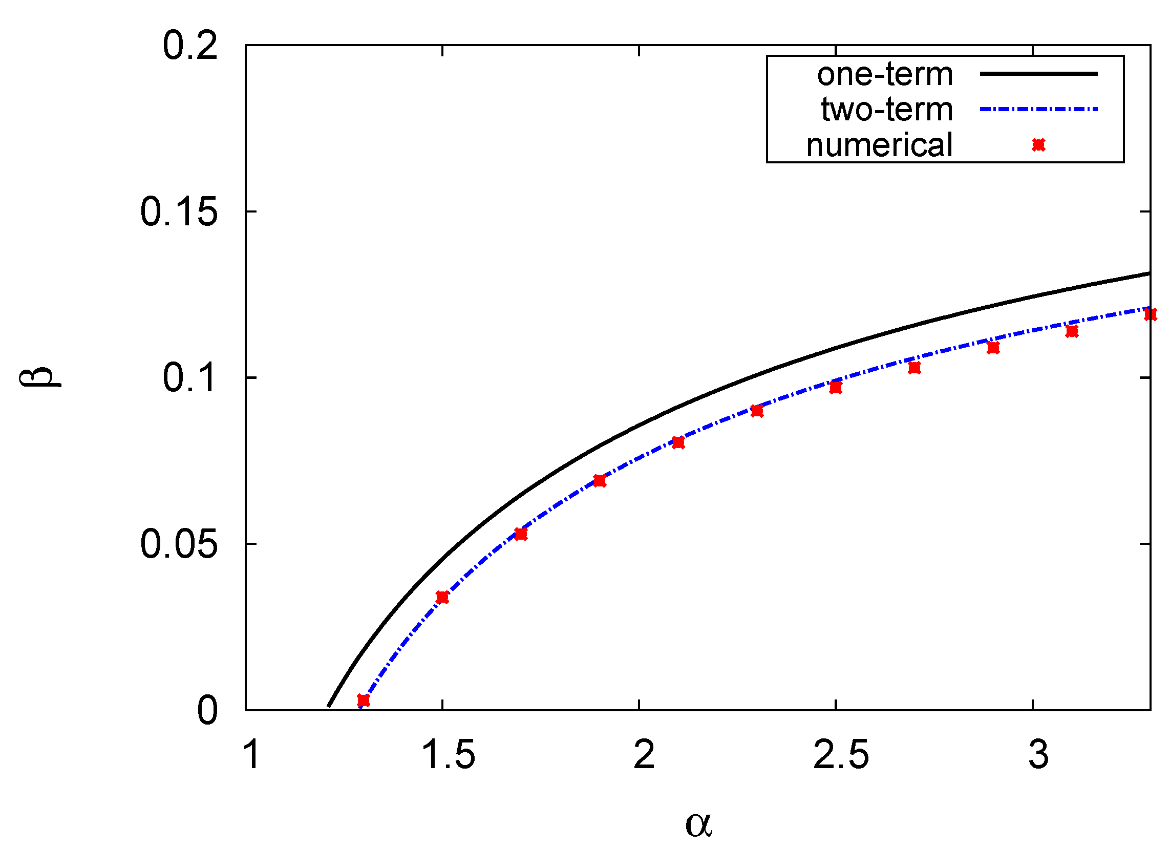
Figure 4 depicts the Hopf bifurcation curve map of the prey growth rate $\alpha$ versus the predator mortality rate $\beta$. The results of the one- and two-term models, as well as the numerical solution are shown. The parameter values utilised were $\gamma =0.4$, ${\mu }_1={\delta }_3={\kappa }_3=0.5$, ${\mu }_2={\delta }_2={\kappa }_2=0.3$, ${\mu }_3={\delta }_1={\kappa }_1=0.1$, $D_i=0.05$, and ${\tau }_i=1;i=1,2,3$. In this figure, there are two portions, as shown below. The upper portion of the Hopf bifurcation curve represents a stable region, whereas the lower portion of the curve represents an unstable region. In general, the increase in the growth rate of the prey $\alpha$ destabilised the system, whereas the increase in the mortality rate of the predator $\beta$ stabilised it, and this is in agreement with what was mentioned in [49]. The Hopf bifurcation points can only occur for $\alpha \ge 1.21$ and $1.29$ for the one-term and two-term methods, respectively. Comparison of the two-term results with the numerical solution of system (1) and (2) revealed close concordance. As such, at $\alpha =2.3$, the numerical estimate at which Hopf bifurcations can occur is $\beta =0.088$, whereas the one- and two-term values are $\beta =0.102$ and $0.091$, respectively, with errors of 16 and $3.5\%$.

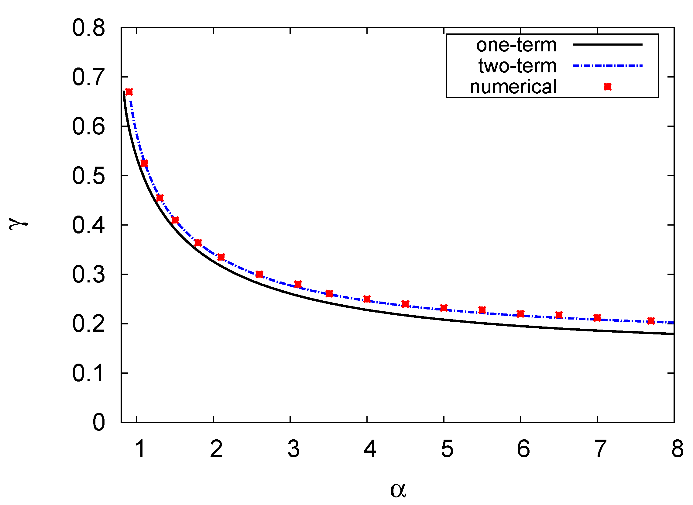
Figure 5 further shows the Hopf bifurcation curve in the $\alpha$–$\gamma$ plane. The figure illustrates the one- and two-term model results with the numerical solution of the PDE system. The other parameters are the same as those in Figure 4, and $\beta =0.04$. Once again, the Hopf bifurcation curve divides the plane into upper and lower parts. Limit cycles and unstable solutions occur at the top, whilst limit cycles disappear and stable solutions occur below the curve. The results in the figure show that the increase in the growth rate $\alpha$ of the prey is offset by the decrease in the mortality rate $\gamma$ of the top predator. In other words, the increase in the growth rate of the prey and mortality rate of the top predator destabilise the system. There was a close concordance between the results of the two-term model and the numerical solution, with an error of <2%.

In Figure 6, the effects of hunting and maturation time delay of the three species on the stability of the system are examined. Figure 6a,b present the Hopf bifurcation curves in the $\alpha$-$\beta$ and $\alpha$-$\gamma$ planes, respectively, at different values of ${\tau }_i=1,1.2$, and $1.5$, $(i=1,\dots ,3)$. Results of the two-term method are shown. The other variables are the same as those in Figure 4 and Figure 5. The results show that the increase in time delay shifts the Hopf bifurcation curve upward in the $\alpha$–$\beta$ and downward in the in the $\alpha$–$\gamma$ domain. As a result of this increase, the zones of the limit cycle broadened and the stable solutions decline, leading to system destabilisation. For instance, the points $(\alpha ,\beta )=(2,1.5)$ and $(\alpha ,\gamma )=(5,0.1)$ are stable at ${\tau }_i=1$ but not at ${\tau }_i=1.2$ and $1.5$, $i=1,2,3$.

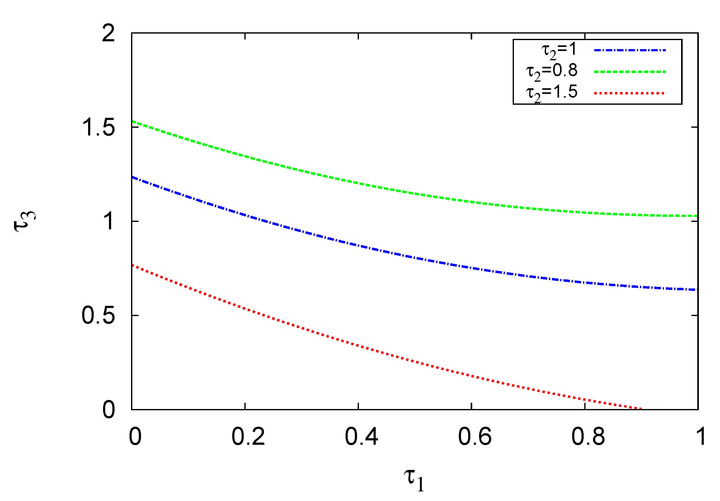
Figure 7 depicts the regions in the ${\tau }_1$-${\tau }_3$ phase plane where Hopf bifurcation occurs. The two-term solutions at different values of ${\tau }_2=0.8$, 1, and $1.5$ are demonstrated. The set of the parameters are $\alpha =2$ and $\beta =0.04$, and the other parameters are the same as those in Figure 4. The curves separate the plane into two parts: upper and lower. Limit cycles and unstable solutions occur above the curves, whereas only stable solutions occur below them. The figure also exhibits that the increase in the delay in the maturation time of the top predator extends the zone of instability of the system. Generally, small delays result in stability whereas large delays, which suggest feedback from the distant past, result in instability [1,14].

The diffusion coefficients play an important role in determining species persistence and extinction [52]. Figure 8 exhibits the Hopf bifurcation regions for the two-term method in the $D_1$-$D_2$ phase plane at different values of diffusion coefficient ($D_3=0.02,0.05$, and $0.1$). The parameter values are $\alpha =2$ and $\beta =0.02$, and the other parameters are the same as those in Figure 4. Here, the inside region shows the oscillating solutions and the limit cycles, whilst the outside region shows the stable solutions. In addition, as the value of the diffusion coefficient for the top predator ($D_3$) increases, the system dynamics vary from stable solution to limit cycle. Briefly, the alteration of the diffusion coefficients rendered the system either stable or unstable [50,51].

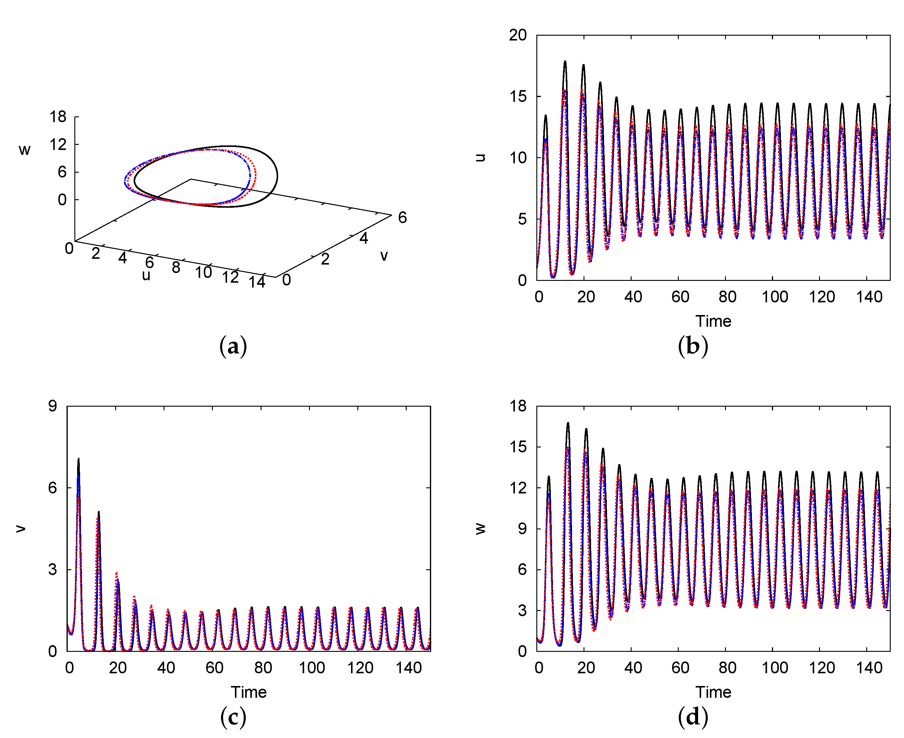
Figure 9a depicts the limit cycle in the $3-D$ phase plane for the density of the prey $\left(u\right)$, predator $\left(v\right)$, and top predator $\left(w\right)$, and Figure 9b–d indicate the evolution of the population densities of u, v, and w, respectively, versus time at $x=0$. Here, $\alpha =1.8$ and $\beta =0.02$, and the other parameters are the same as those in Figure 4. The parameters applied in this case correspond to the zone below the Hopf bifurcation curve in Figure 4, resulting in a limit cycle. The figures present the solutions of both one- and two-term methods, as well as the numerical solution of system (1) and (2). The limit cycle period in the numerical solution was estimated to be $6.84$, whilst those in the one- and two-term methods were $6.86$ and $6.85$, respectively. Moreover, the limit cycle amplitudes of the species were $(u,v,w)=(9.155,1.517,8.70)$ (numerical), $(u,v,w)=(10.342,1.561,9.842)$ (one-term), and $(u,v,w)=(8.995,1.492,8.634)$ (two-term), at the centre of the domain at $x=0$.

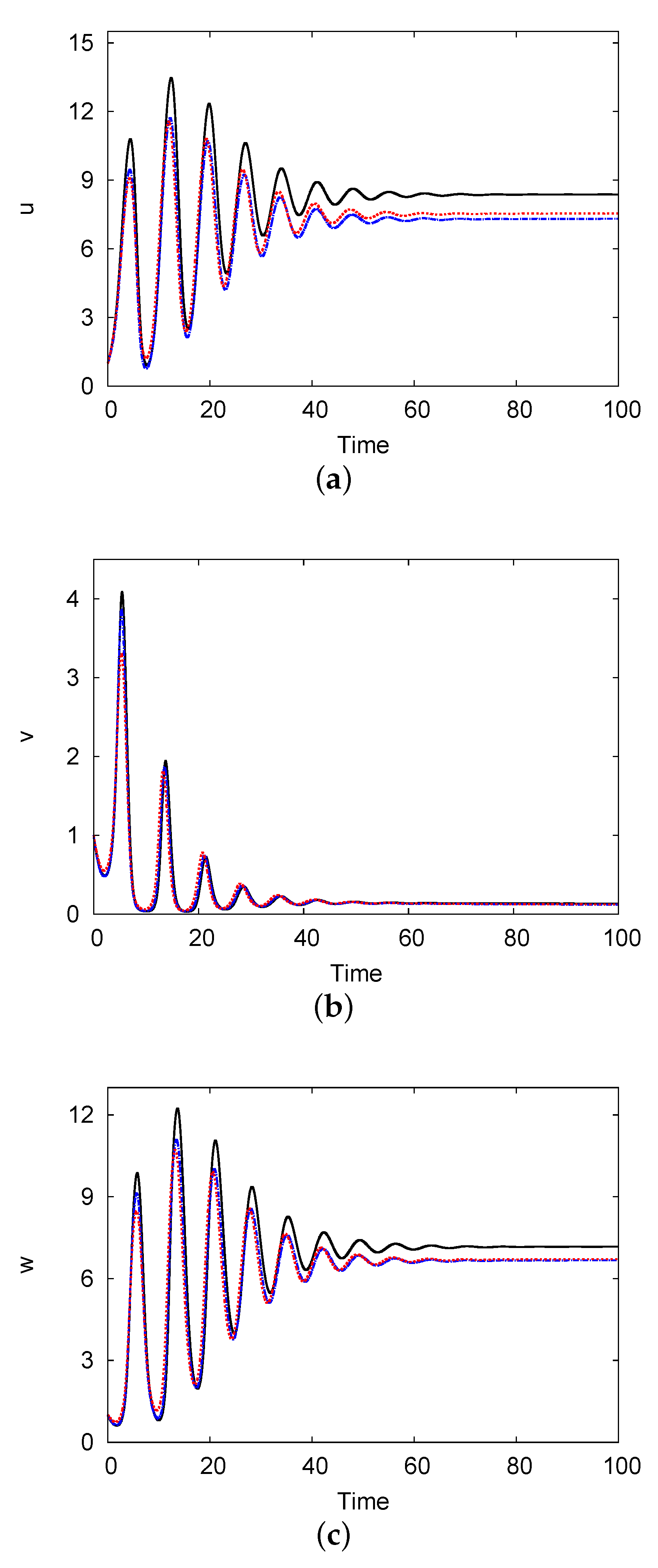
Figure 10 demonstrates the evolution of the population density of the prey u$\left(a\right)$, predator v$\left(b\right)$, and top predator w$\left(c\right)$ versus time at domain centre with $x=0$. It exhibits the one-term and two-term results in addition to the numerical solution of system (1) and (2). The parameter values are $\alpha =1.5$ and $\beta =0.15$, and the other parameters are the same as those in Figure 4. Since all parameters are located above the Hopf bifurcation curve in Figure 4, a stable solution is possible. When the time is sufficient $(t>60)$, the solution of the system converges to a coexistence steady state. This coexistence steady-state solution is given by $(u,v,t)=(8.37,0.133,7.173)$ (one-term), $(u,v,w)=(7.320,0.121,6.678)$ (two-term), and $(u,v,w)=(7.552,0.122,6.719)$ (numerical). These results indicate that the two-term solution is superior to the numerical solution of the PDE system, with an error of <3.1% for all species.

5. Bifurcation Diagrams

Utilisation of a bifurcation diagram is considered a standard way to exhibit behaviour in non-linear dynamic systems including complex periodic and chaotic behaviours [53,54]. This section compares and investigates the dynamics of the PDE system and the semi-analytical DDE model. The bifurcation diagrams indicated long-term solutions for the amplitude of the steady-state branch, as well as the maximum and minimum amplitudes of the oscillatory solutions. As chaotic solutions were obtained for values of the population densities of the three species against the growth rate of the prey $\alpha$, the bifurcation diagrams were drawn at the centre of the domain ($x=0$) for large values of time.

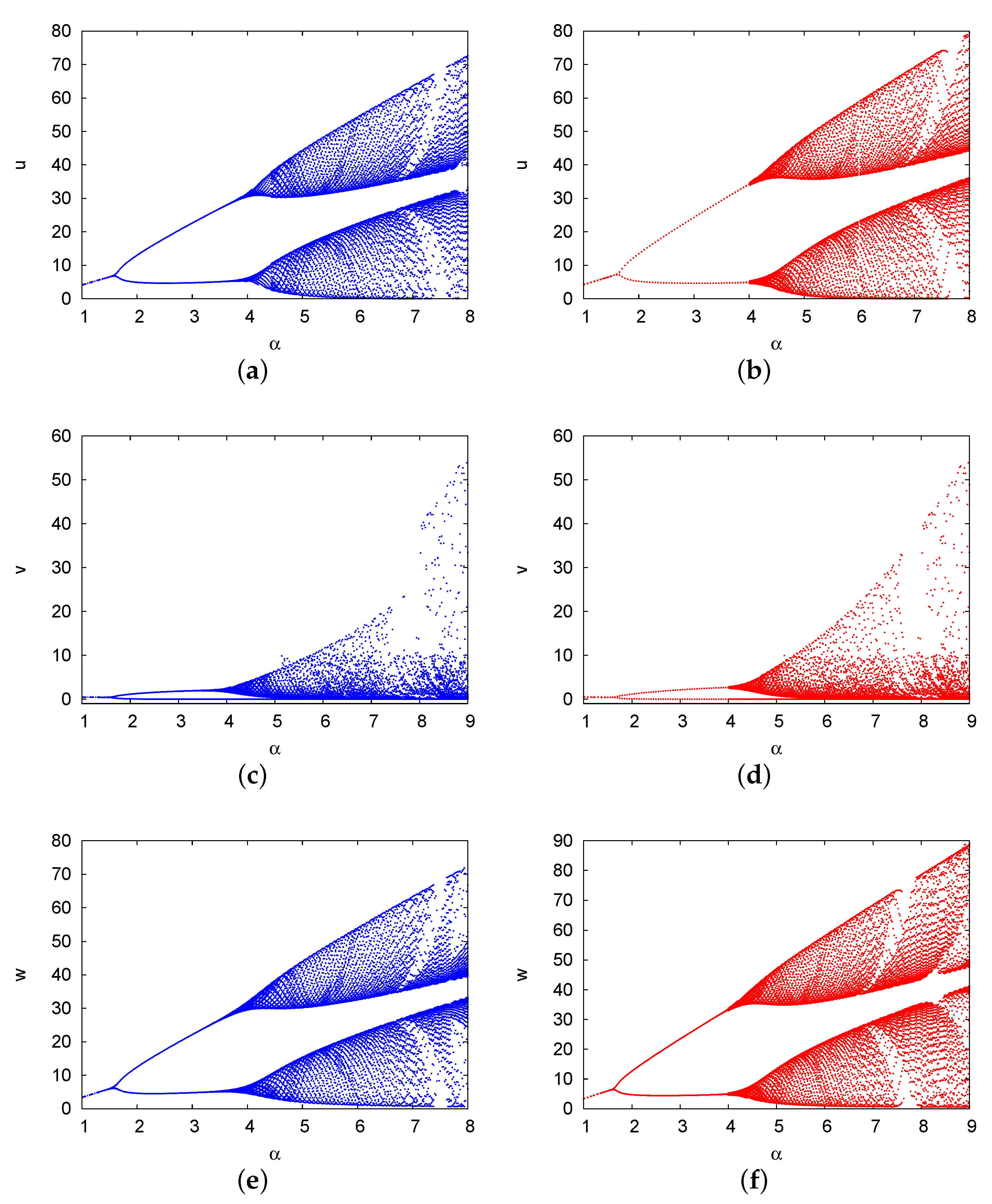
Figure 11 shows the bifurcation diagrams of the population densities of the prey u, predator v, and top predator w versus $\alpha$. $\beta =0.05$, and the other parameters are the same as those in Figure 4. The diagram presents the results of the two-term method for u (Figure 11a), v (Figure 11c), and w (Figure 11e), as well as the PDE numerical solution of the species u (Figure 11b), v (Figure 11d), and w (Figure 11f). In this figure, the system is initially stable at $\alpha <1.63$ and then the Hopf bifurcation occurs at $\alpha =1.63$ (two-term) and $1.64$ (numerical), providing periodic solutions in the range $1.63\le \alpha <4.1$ (two-term) and $1.64\le \alpha <4$ (numerical). At $\alpha =4.1$ (two-term) and 4 (numerical), attracting period-doubling bifurcation occurs. At $\alpha >4.1$, for each branch of the periodic solutions, the system induces a route to chaos, replacing the periodic solution cascades. The estimates of the two-term method were consistent with the numerical results of the PDE system, with an error of $<2.5\%$. In conclusion, the increase in the growth rate of prey in a three-species system may lead to the occurrence of chaotic solutions, as reported previously [55].

6. Conclusions

In this study, the dynamics of a diffusive Lotka–Volterra two predator-prey system with delays were explored. By employing the Galerkin Method, which generates semi-analytical solutions, the PDE system was approximated using a DDE model. Steady-state curves and Hopf bifurcation maps were created and discussed in detail.

The effects of the growth rate of the prey and the mortality rate of the predator and top predator on system stability were demonstrated. As such, an increase in the growth rate of prey destabilised the system, whilst an increase in the mortality of both predator and top predator stabilised the system. In addition, the impact of hunting and maturation delays of the species were examined. Small delays stabilised the system, whilst great delays destabilised it. Furthermore, the effects of the diffusion coefficients of the species were investigated. The alteration of the diffusion coefficients rendered the system either permanent or extinct.

These results can serve as the foundation for future research. The present study demonstrated the high accuracy and utility of the semi-analytical model for studying the dynamics of specific biological systems, such as delayed diffusive multispecies Lotka–Volterra food chains or two-prey/one-predator systems [22]. Furthermore, in the light of harvesting in non-diffusive models [47,49], one more interesting investigation would be to vary the mortality rate as a control parameter, and examine the impacts of harvesting upon the diffusive system (1) and (2).

References

- Alfifi, H.Y.; Marchant, T.R.; Nelson, M.I. Generalised Diffusive Delay Logistic Equations: Semi-analytical solutions. Dyn. Contin. Discret. Ser. B. 2012, 19, 579–596. [Google Scholar]
- Chen, S.; Shi, J. Stability and Hopf bifurcation in a diffusive logistic population model with nonlocal delay effect. J. Differ. Equ. 2012, 12, 3440–3470. [Google Scholar] [CrossRef] [Green Version]
- Su, Y.; Wei, J.; Shi, J. Hopf Bifurcation in a Diffusive Logistic Equation with Mixed Delayed and Instantaneous Density Dependence. J. Dyn. Differ. Equ. 2012, 24, 897–925. [Google Scholar] [CrossRef]
- Alfifi, H. Stability and Hopf bifurcation analysis for the diffusive delay logistic population model with spatially heterogeneous environment. Appl. Math. Comput. 2021, 408, 126362. [Google Scholar] [CrossRef]
- Hastings, A.; Powell, T. Chaos in a Three-Species Food Chain. Ecology 1991, 72, 896–903. [Google Scholar] [CrossRef]
- Song, Y.; Peng, Y.; Wei, J. Bifurcations for a predator-prey system with two delays. J. Math. Anal. Appl. 2008, 337, 466–479. [Google Scholar] [CrossRef] [Green Version]
- Yang, R.; Zhang, C. Dynamics in a diffusive predator-prey system with a constant prey refuge and delay. Nonlinear Anal. Real World Appl. 2016, 31, 1–22. [Google Scholar] [CrossRef]
- Lotka, A. Elements of Physical Biology; Williams & Wilkins Company: Baltimore, MD, USA, 1925. [Google Scholar]
- Hacinliyan, A.S.; Kusbeyzi, I.; Aybar, O.O. Approximate solutions of Maxwell Bloch equations and possible Lotka-Volterra type behavior. Nonlinear Dyn. 2010, 62, 17–26. [Google Scholar] [CrossRef]
- Faria, T. Stability and bifurcation for a delayed predator-prey model and the effect of diffusion. Math. Anal. Appl. 2001, 254, 433–463. [Google Scholar] [CrossRef] [Green Version]
- Yan, X.; Chu, Y. Stability and bifurcation analysis for a delayed Lotka-Volterra predator-prey system. Comput. Appl. Math. 2006, 196, 198–210. [Google Scholar] [CrossRef] [Green Version]
- Chen, S.; Shi, J.; Wei, J. A note on Hopf bifurcations in a delayed diffusive Lotka-Volterra predator-prey system. Comput. Math. Appl. 2011, 62, 2240–2245. [Google Scholar] [CrossRef] [Green Version]
- Tahara, T.; Gavina, M.; Kawano, T.; Tubay, J.; Rabajante, J.; Ito, H.; Morita, S.; Ichinose, G.; Okabe, T.; Togashi, T.; et al. Asymptotic stability of a modified Lotka-Volterra model with small immigrations. Sci. Rep. 2018, 8, 7029. [Google Scholar] [CrossRef] [PubMed]
- Al Noufaey, K.S.; Marchant, T.R.; Edwards, M.P. Semi-analytical solutions for the diffusive Lotka-Volterra predator-prey system with delay. Math. Biosci. 2015, 270, 30–40. [Google Scholar] [CrossRef] [PubMed] [Green Version]
- Shenghu, X. Dynamics of a general prey-predator model with prey-stage structure and diffusive effects. Comput. Math. Appl. 2014, 68, 405–423. [Google Scholar]
- Alsakaji, H.J.; Kundu, S.; Rihan, F.A. Delay differential model of one-predator two-prey system with Monod-Haldane and holling type II functional responses. Appl. Math. Comput. 2021, 397, 125919. [Google Scholar] [CrossRef]
- Gakkhar, S.; Naji, R. Chaos in three species ratio dependent food chain. Chaos Solitons Fractalas 2002, 14, 771–778. [Google Scholar] [CrossRef]
- Gilpin, M.E. Spiral chaos in a predator-prey model. Am. Nat. 1979, 107, 306–308. [Google Scholar] [CrossRef]
- Mbava, W.; Mugisha, J.; Gonsalves, J. Prey, predator and super-predator model with disease in the super-predator. Appl. Math. Comput. 2017, 297, 92–114. [Google Scholar] [CrossRef]
- Schaffer, W. Order and chaos in ecological systems. Ecology 1995, 66, 93–106. [Google Scholar] [CrossRef]
- Naji, R.K.; Balasim, A.T. Dynamical behavior of a three species food chain model with Beddington-DeAngelis functional response. Chaos Solitons Fractals 1995, 32, 1853–1866. [Google Scholar] [CrossRef]
- Pao, C. Global asymptotic stability of Lotka-Volterra 3-species reaction-diffusion systems with time delays. J. Math. Anal. Appl. 2003, 281, 186–204. [Google Scholar] [CrossRef] [Green Version]
- Liao, M.; Tang, X.; Xu, C. Dynamics of a competitive Lotka-Volterra system with three delays. Appl. Math. Comput. 2011, 217, 10024–10034. [Google Scholar] [CrossRef]
- Klebanoff, A.; Hastings, A. Chaos in three-species food chains. J. Math. Biol. 1994, 32, 427–451. [Google Scholar] [CrossRef]
- Zhao, M.; Lv, S. Chaos in a three-species food chain model with a Beddington-DeAngelis functional response. Chaos, Solitons Fractals 2009, 40, 2305–2316. [Google Scholar] [CrossRef]
- Thompson, H.B.; Do, Y.; Baek, H.; Lim, Y.; Lim, D. A Three-Species Food Chain System with Two Types of Functional Responses. Abstr. Appl. Anal. 2011, 2011, 1–16. [Google Scholar]
- Galerkin, B.G. Rods and plates. Series occurring in various questions concerning the elastic equilibrium of rods and plates. Eng. Bull. (Vestn. Inszh. Tech.) 1915, 19, 897–908. [Google Scholar]
- Marchant, T.R. Cubic autocatalytic reaction-diffusion equations: Semi-analytical solutions. Proc. R. Soc. Lond. A 2002, 458, 873–888. [Google Scholar] [CrossRef] [Green Version]
- Al Noufaey, K.S. Semi-analytical solutions of the Schnakenberg model of a reaction-diffusion cell with feedback. Results Phys 2018, 9, 609–614. [Google Scholar] [CrossRef]
- Al Noufaey, K.S. A semi-analytical approach for the reversible Schnakenberg reaction-diffusion system. Results Phys 2020, 16, 102858. [Google Scholar] [CrossRef]
- Al Noufaey, K.S. Stability analysis for Selkov-Schnakenberg reaction-diffusion system. Open Math. 2021, 19, 46–62. [Google Scholar] [CrossRef]
- Al Noufaey, K.S.; Marchant, T.R. Semi-analytical solutions for the reversible Selkov model with feedback delay. Appl. Math. Comput. 2014, 232, 49–59. [Google Scholar] [CrossRef] [Green Version]
- Al Noufaey, K.S.; Marchant, T.R.; Edwards, M.P. A semi-analytical analysis of the stability of the reversible Selkov model. Dynam. Cont. Dis. Ser. B. 2015, 22, 117–139. [Google Scholar]
- Alfifi, H. Semi-analytical solutions for the diffusive logistic equation with mixed instantaneous and delayed density dependence. Adv. Differ. Equ. 2020, 162. [Google Scholar] [CrossRef]
- Alfifi, H.Y. Semi-analytical solutions for the Brusselator reaction-diffusion model. ANZIAM J. 2017, 59, 167–182. [Google Scholar] [CrossRef]
- Alfifi, H.Y. Feedback Control for a Diffusive and Delayed Brusselator Model: Semi-Analytical Solutions. Symmetry 2021, 13, 725. [Google Scholar] [CrossRef]
- Alfifi, H.Y.; Marchant, T.R.; Nelson, M.I. Semi-analytical solutions for the 1 and 2-D diffusive Nicholson’s blowflies equation. IMA J. Appl. Math. 2012, 79, 175–199. [Google Scholar] [CrossRef]
- Alharthi, M.R.; Marchant, T.R.; Nelson, M.I. Semi-analytical solutions for cubic autocatalytic reaction-diffusion equations; the effect of a precursor chemical. ANZIAM J. 2012, 53, C511–C524. [Google Scholar] [CrossRef] [Green Version]
- Alharthi, M.R.; Marchant, T.R.; Nelson, M.I. Mixed quadratic-cubic autocatalytic reaction-diffusion equations: Semi-analytical solutions. Appl. Math. Model. 2014, 38, 5160–5173. [Google Scholar] [CrossRef]
- Marchant, T.R. Cubic autocatalysis with Michaelis-Menten kinetics: Semi-analytical solutions for the reaction-diffusion cell. Chem. Eng. Sci. 2004, 59, 3433–3440. [Google Scholar] [CrossRef]
- Marchant, T.R.; Nelson, M.I. Semi-analytical solutions for one and two-dimensional pellet problems. Proc. Roy. Soc. Lond. A 2004, 460, 2381–2394. [Google Scholar] [CrossRef]
- Fagan, W.F.; Cantrell, R.S.; Cosner, C. How habitat edges change species interactions. Am. Nat. 1999, 153, 165–182. [Google Scholar] [CrossRef]
- Golubitsky, M.; Schaeffer, D.G. Singularites and Groups in Bifurcation Theory; Springer: New York, NY, USA, 1985. [Google Scholar]
- Guckenheimer, J.; Holmes, P. Nonlinear Oscillations, Dynamical Systems, and Bifurcations of Vector Fields; Springer: New York, NY, USA, 1983. [Google Scholar]
- Ruan, S.; Wei, J. On the zeros of transcendental functions with applications to stability of delay differential equations with two delays. Dyn. Contin. Discret. Impuls. Syst. Ser. B Appl. Algorithms 2003, 10, 863–874. [Google Scholar]
- Gu, K.; Niculescu, S.; Chen, J. On stability crossing curves for general systemswith two delays. J. Math. Anal. Appl. 2005, 311, 231–253. [Google Scholar] [CrossRef] [Green Version]
- Barman, B.; Ghosh, B. Explicit impacts of harvesting in delayed predator-prey models. Chaos Solitons Fractals 2019, 122, 213–228. [Google Scholar] [CrossRef]
- Barman, B.; Ghosh, B. Dynamics of a spatially coupled model with delayed prey dispersal. Int. J. Model. Simul. 2021, 1–15. [Google Scholar] [CrossRef]
- Barman, B.; Ghosh, B. Role of time delay and harvesting in some predator-prey communities with different functional responses and intra-species competition. Int. J. Model. Simul. 2021, 1–19. [Google Scholar] [CrossRef]
- Ji, J.; Lin, G.; Wang, L. Effects of intraguild prey dispersal driven by intraguild predator-avoidance on species coexistence. Appl. Math. Model. 2021, 103, 51–67. [Google Scholar] [CrossRef]
- Bajeux, N.; Ghosh, B. Stability switching and hydra effect in a predator-prey metapopulation model. Biosystems. 2020, 198, 104255. [Google Scholar] [CrossRef]
- Cui, J.A.; Chen, L. The effect of diffusion on the time varying logistic population growth. Comput. Math. Appl. 1998, 36, 1–9. [Google Scholar] [CrossRef] [Green Version]
- Glendinning, P. Stability, Instability and Chaos: An Introduction to the Theory of Nonlinear Differential Equations; Cambridge University Press: Cambridge, UK, 1994. [Google Scholar]
- Guckenheimer, J.; Holmes, P. Nonlinear Dynamics and Chaos; John Wiley and Sons: Chichester, UK, 1986. [Google Scholar]
- Kozlov, V.; Vakulenko, S. On chaos in Lotka-Volterra systems: An analytical approach. Nonlinearity 2013, 26, 2299–2314. [Google Scholar] [CrossRef]
Figure 1.
Steady–state population density profiles of the prey u (a), the predator v (b), and the top predator w (c) versus x. The parameters used include , , , , , , and . The figure represents the one-term (black solid line) and two-term (blue dashed line) methods and the numerical solution (blue dashed line) of PDE.
Figure 2.
Steady–state population density profiles of the prey u (a), the predator v (b), and the top predator w (c) versus x at different growth rates ( (green line), (blue line), and 2 (black line). It exhibits the two-term solutions. The parameters used here are the same as those used in Figure 1.
Figure 3.
Steady-state population density profiles of the prey u (a), the predator v (b), and the top predator w (c) versus the prey growth rate . This figure demonstrates the solutions of the one-term (black solid line) and two-term (blue dashed line) methods, as well as the numerical solution (red dotted line) with the group of other feasible parameter values shown in Figure 1.
Figure 4.
Hopf bifurcation map in the phase plane of the prey growth rate and the predator mortality rate . The parameters values are , , , , , and .
Figure 5.
Hopf bifurcation map showing in the phase plane of the prey growth rate versus the mortality rate of the top predator . Here, and the other parameter values are the same as those in Figure 4.
Figure 6.
Hopf bifurcation curves appearing within the - (a) and - (b) phase planes. The solutions of the two-term method at different values of , are illustrated. The other parameter values are given in Figure 4 and Figure 5, respectively.
Figure 7.
Hopf bifurcation curves within the - phase plane at different values of . The results of the two-term method are shown. The parameter values are and , and the other parameters are the same as those in Figure 4.
Figure 8.
Stability regions constructed by the Hopf bifurcation curves within the - phase plane at different values of . The results of the two-term method are shown. The parameter values are and , and the other parameters are the same as those in Figure 4.
Figure 9.
Phase portrait of the system showing the limit cycle (a) and the oscillations of the species u (b), v (c), and w (d) in the time evolution, respectively, at . The one-term and two-term method solutions are represented by black solid and blue dashed lines, respectively, whilst the numerical solution is represented by the red dotted lines. The parameter values are and , and the other parameters are the same as those in Figure 4.
Figure 10.
Evolution of the population density of the prey u (a), predator v (b), and top predator w (c) versus time at the domain centre with . The results of the one-term (black solid line) and two-term (blue dashed line) methods as well as of the numerical solution (red dotted line) are shown. The parameter values are and , and the other parameters are the same as those in Figure 4.
Figure 11.
Bifurcation diagrams of the population densities of the prey u, predator v, and top predator w against . The diagram presents the results of the two-term method for u (a), v (c), and w (e), as well as the PDE numerical solutions for the species u (b), v (d), and w (f). , and the other parameters are the same as those in Figure 4.
Publisher’s Note: MDPI stays neutral with regard to jurisdictional claims in published maps and institutional affiliations. |
© 2021 by the author. Licensee MDPI, Basel, Switzerland. This article is an open access article distributed under the terms and conditions of the Creative Commons Attribution (CC BY) license (https://creativecommons.org/licenses/by/4.0/).
Share and Cite
MDPI and ACS Style
Al Noufaey, K.S. Stability Analysis of a Diffusive Three-Species Ecological System with Time Delays. Symmetry 2021, 13, 2217. https://0-doi-org.brum.beds.ac.uk/10.3390/sym13112217
AMA Style
Al Noufaey KS. Stability Analysis of a Diffusive Three-Species Ecological System with Time Delays. Symmetry. 2021; 13(11):2217. https://0-doi-org.brum.beds.ac.uk/10.3390/sym13112217
Chicago/Turabian StyleAl Noufaey, Khaled S. 2021. "Stability Analysis of a Diffusive Three-Species Ecological System with Time Delays" Symmetry 13, no. 11: 2217. https://0-doi-org.brum.beds.ac.uk/10.3390/sym13112217
Note that from the first issue of 2016, this journal uses article numbers instead of page numbers. See further details here.