First Principles Calculation of the Topological Phases of the Photonic Haldane Model

Abstract

Photonic topological materials with a broken time-reversal symmetry are characterized by nontrivial topological phases, such that they do not support propagation in the bulk region but forcibly support a nontrivial net number of unidirectional edge-states when enclosed by an opaque-type boundary, e.g., an electric wall. The Haldane model played a central role in the development of topological methods in condensed-matter systems, as it unveiled that a broken time-reversal symmetry is the essential ingredient to have a quantized electronic Hall phase. Recently, it was proved that the magnetic field of the Haldane model can be imitated in photonics with a spatially varying pseudo-Tellegen coupling. Here, we use Green’s function method to determine from “first principles” the band diagram and the topological invariants of the photonic Haldane model, implemented as a Tellegen photonic crystal. Furthermore, the topological phase diagram of the system is found, and it is shown with first principles calculations that the granular structure of the photonic crystal can create nontrivial phase transitions controlled by the amplitude of the pseudo-Tellegen parameter.

1. Introduction

The study of topological properties of physical systems and of how the topology influences the physical responses and phenomena has been a very active field of research in recent years [1,2,3,4,5,6,7,8,9,10,11,12,13,14,15,16,17,18,19]. The topology of physical systems is typically determined by the global properties of the operator that describes the time evolution of the system state (in quantum systems, this operator is the Hamiltonian). Here, we focus on a particular class of topological systems known as Chern insulators [7]. Such systems have a broken time reversal symmetry and are characterized by a topological invariant known as the Chern number. The key fingerprint of a nontrivial topological phase is the emergence of gapless scattering immune unidirectional edge-states at the boundary of the material. This property makes the response of topological systems rather insensitive to fabrication imperfections, disorder and other perturbations [9].

In the 1980s, Haldane discovered that electronic systems with a broken time-reversal symmetry (e.g., an electron gas biased with a magnetic field) may have a quantized Hall conductivity, even if the spatial-average of the magnetic field vanishes [2]. The Haldane model is essentially a tight-binding description of the propagation of an electron wave in a honeycomb lattice of scattering centers (electric potential interaction), subject also to the influence of a periodic magnetic vector potential. The periodicity of the vector potential ensures that the net magnetic flux in a unit cell vanishes. Sometime ago, it was shown that the model theoretically envisioned by Haldane may be implemented in practice using an “artificial graphene” superlattice biased with a spatially varying magnetic field [20,21]. Moreover, a photonic analogue for the Haldane model was developed in [22], with the magnetic field of the original electronic model imitated by a spatially varying pseudo-Tellegen coupling. In Reference [22], the topological phases of the photonic system were determined relying on a tight-binding approximation. Here, building on these previous works, we use an exact Green’s function method [19,23,24,25] to calculate from “first principles” the topological invariants of the Haldane photonic crystal.

The article is organized as follows. In Section 2, we present a brief overview of the electronic Haldane model and of its electromagnetic analogue. In Section 3, the Green’s function formalism is applied to the electronic (tight-binding) Haldane model and to the Haldane photonic crystal formed by materials with a pseudo-Tellegen response. In Section 3, the topological phases of the electronic and photonic models are calculated based on a Green’s function approach. A short summary of the key results is given in Section 4.

2. The Haldane Model

In this section, we briefly review the original Haldane model and its electromagnetic analogue [2,21,22].

2.1. The Electronic Haldane Model

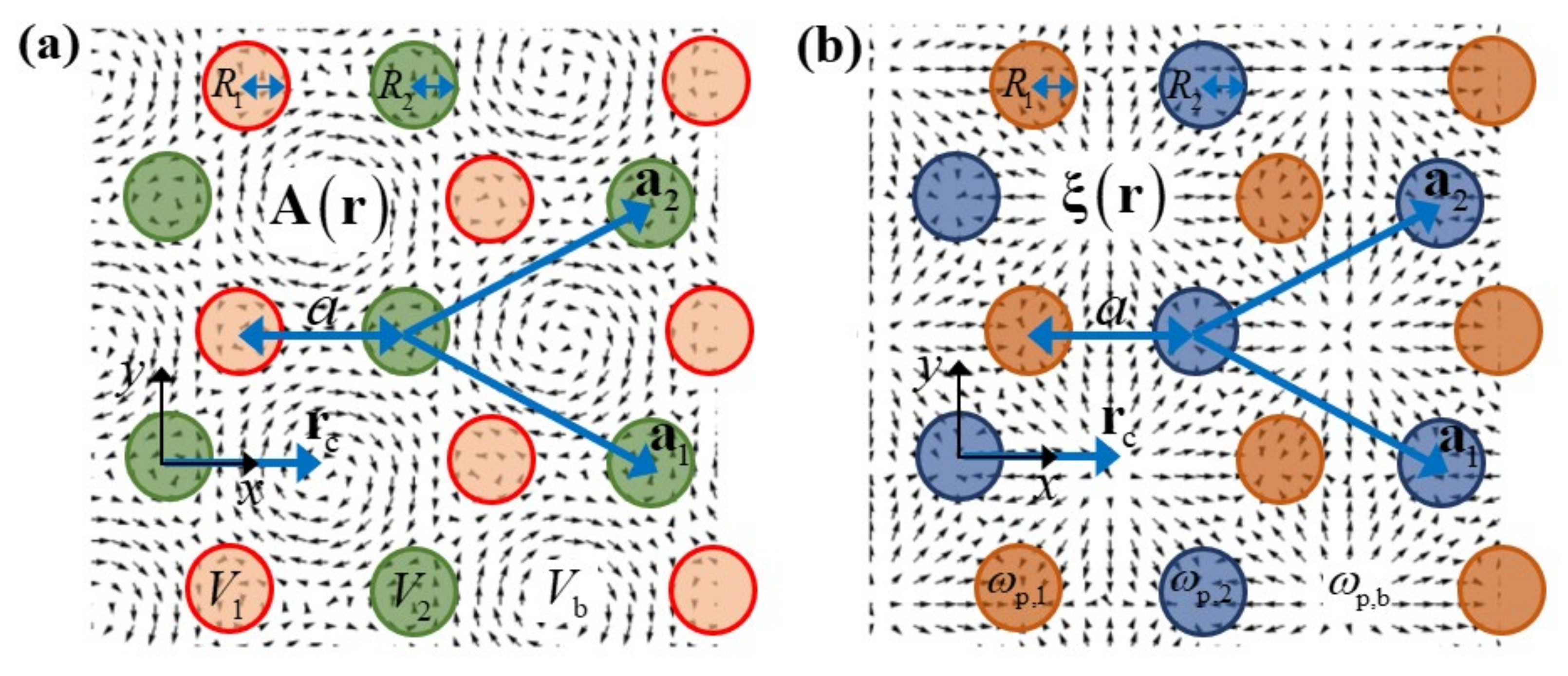
The Haldane model [2] describes the electronic stationary states of a hexagonal two-dimensional array of scattering centers under the influence of a static magnetic field with a vanishing net flux (Figure 1a). There are two inequivalent scattering centers per unit cell, analogous to graphene. The direct lattice primitive vectors are $a_1=a/2\left(3,-\sqrt{3}\right)$ and $a_2=a/2\left(3,\sqrt{3}\right)$, where a is the distance between nearest neighbors (Figure 1a). In a tight-binding approximation, the Hamiltonian of the Haldane model in the spectral domain is determined by the 2 × 2 matrix:

$$H\left(k\right)=\epsilon \left(k\right)1+d_x\left(k\right){\sigma }_x+d_y\left(k\right){\sigma }_y+d_z\left(k\right){\sigma }_z.$$

(1)

In the above, ${\sigma }_i$ are the Pauli matrices and the relevant coefficients are:

$$\begin{array}{l}\epsilon \left(k\right)=2t_2\cos \left(\varphi \right)\left[\cos \left(k\cdot a_1\right)+\cos \left(k\cdot a_2\right)+\cos \left(k\cdot \left(a_2-a_1\right)\right)\right]\\ d_x\left(k\right)=t_1\left[2\cos \left(k_x\frac{a}{2}\right)\cos \left(k_{y}a\frac{\sqrt{3}}{2}\right)+\cos \left(k_{x}a\right)\right]\\ d_y\left(k\right)=t_1\left[2\sin \left(k_x\frac{a}{2}\right)\cos \left(k_{y}a\frac{\sqrt{3}}{2}\right)-\sin \left(k_{x}a\right)\right]\\ d_z\left(k\right)=M-2t_2\sin \left(\varphi \right)\left[\sin \left(k\cdot a_1\right)-\sin \left(k\cdot a_2\right)+\sin \left(k\cdot \left(a_2-a_1\right)\right)\right]\end{array}$$

(2)

Here, $t_1$ and $t_2$ are the nearest-neighbors and next-nearest neighbors hopping energies, respectively, $M$ is the so-called “mass term” and $\varphi$ is the phase factor determined by the coupling between next-nearest neighbors due to the applied magnetic potential. The parameter $M$ is nonzero when the scattering centers associated with the different sub-lattices are different.

The Hamiltonian $H\left(k\right)$ acts on a two-component pseudo-spinor. The components of the pseudo-spinor represent the (Fourier) coordinates of the wave function in the tight-binding basis. The energy dispersion is determined by $\det \left(H-\mathcal{E}1\right)=0$, which yields exactly two electronic bands: ${\mathcal{E}}_k^{\pm }\left(k\right)=\epsilon \pm \sqrt{d_x^2+d_y^2+d_z^2}$. The wave vector is defined over the first Brillouin zone. The primitive vectors of the reciprocal lattice are:

$$b_1=\frac{2\pi }{a}\left(\frac{1}{3},-\frac{1}{\sqrt{3}}\right),\hspace{1em}{b}_2=\frac{2\pi }{a}\left(\frac{1}{3},\frac{1}{\sqrt{3}}\right).$$

(3)

The energy bands ${\mathcal{E}}_k^{\pm }\left(k\right)$ can touch only if $d_x\left(k\right)=d_y\left(k\right)=d_z\left(k\right)=0$. The only points of the Brillouin zone that may satisfy $d_x\left(k\right)=d_y\left(k\right)=0$ are the two high symmetry (Dirac) points:

$$K=\frac{2\pi }{3a}\left(1,\frac{1}{\sqrt{3}}\right),\hspace{1em}{K}^{\prime }=\frac{2\pi }{3a}\left(1,-\frac{1}{\sqrt{3}}\right).$$

(4)

Thus, in the Haldane model, the two bands are typically separated by a complete bandgap unless they touch at one of the Dirac points. Below, we show that for large values of $t_2$ the bandgap may be closed, even if the two bands do not intersect.

Reference [21] introduced a possible physical realization of the Haldane model. It relies on a 2D electron gas superlattice patterned with scattering centers, whose effect is modeled by a periodic electric potential $V\left(r\right)$. The electric potential is equal to $V_{\mathrm{b}}$ in the background region and is equal to $V_1$ or $V_2$ in each scattering center (disk) sublattice. A periodic spatially varying magnetic field $B\left(r\right)=\nabla \times A$ determined by the vector potential

$$A(r)=\frac{3B_0{a}^2}{16{\pi }^2}\left[b_1\sin \left(b_1\cdot R\right)+b_2\sin \left(b_2\cdot R\right)+\left(b_1+b_2\right)\sin \left(\left[b_1+b_2\right]\cdot R\right)\right]\times \widehat{z},$$

(5)

is also applied to the system. Here a is the distance between the nearest scattering centers in the hexagonal lattice, $B_0$ is the peak magnetic field in Tesla, $b_1$ and $b_2$ are the reciprocal lattice primitive vectors and $R=r-r_c$ where $r_c=1/3(a_1+a_2)$ determines the coordinates of the honeycomb cell’s center (Figure 1a). The two scatterers are centered at $r_{0,1}=-a\widehat{x}$ and $r_{0,2}=0$, respectively, and have radii $R_1$ and $R_2$.

The stationary states of the (spinless) electronic system are the solutions of the time-independent scalar Schrödinger equation:

$$\left[\frac{-{\hslash }^2}{2m_b}{\left(\nabla +i\frac{e}{\hslash }A(r)\right)}^2+V\left(r\right)-E\right]\Psi =0,$$

(6)

where $\Psi$ is the wavefunction, $m_b$ is the electron effective mass, $e$ is the elementary charge and $\hslash$ is the Planck constant.

2.2. Photonic Analogue of the Haldane Model

It was shown in References [22,26] that a pseudo-Tellegen coupling is the counterpart for photons of the magnetic field coupling for electrons. Specifically, consider a bianisotropic material described by constitutive relations of the type:

$$\left(\begin{array}{c}D\\ B\end{array}\right)=M\cdot \left(\begin{array}{c}E\\ H\end{array}\right), \mathrm{with} M=\left(\begin{array}{cc}{\epsilon }_0\overline{\epsilon }& \frac{1}{c}\overline{\xi }\\ \frac{1}{c}\overline{\zeta }& {\mu }_0\overline{\mu }\end{array}\right),$$

(7)

where $\overline{\epsilon }$, $\overline{\mu }$, $\overline{\xi }$ and $\overline{\zeta }$ are the relative permittivity, permeability and magnetoelectric tensors, respectively. For a pseudo-Tellegen response, the magnetoelectric tensors are identical ($\overline{\zeta }=\overline{\xi }$), symmetric ($\overline{\xi }={\overline{\xi }}^T$) and have zero trace ($\mathrm{tr}\left(\overline{\xi }\right)=0$) [27]. In this article, we assume that the relevant tensors are of the form:

$$\overline{\xi }=\overline{\zeta }=\xi \otimes \widehat{z}+\widehat{z}\otimes \xi ,$$

(8)

where $\xi ={\xi }_x\widehat{x}+{\xi }_y\widehat{y}$ is a generic vector lying in the xoy plane. We will refer to $\xi$ as the pseudo-Tellegen vector. Some anti-ferromagnets such as Cr₂O₃ have a Tellegen-type response, albeit it is typically very weak [28,29,30]. Furthermore, it has been recently shown that some electronic topological insulators may be characterized by a Tellegen type (axion) response [30,31,32,33,34]. Materials with a Tellegen response are nonreciprocal and enable peculiar effects and exotic physics [34,35,36,37]. It is interesting to point out that the Tellegen coupling is real-valued. This means that any homogeneous Tellegen material is certainly topologically trivial. Furthermore, it is worth noting that most of the solutions that yield nontrivial photonic topologies rely on gyrotropic materials with a complex-valued material response, very different from the Tellegen case.

Suppose that the relativity permittivity and permeability tensors are of the form

$$\begin{array}{l}\overline{\epsilon }={\epsilon }_{\parallel }\left(\widehat{x}\otimes \widehat{x}+\widehat{y}\otimes \widehat{y}\right)+{\epsilon }_{zz}\hspace{0.17em}\widehat{z}\otimes \widehat{z}\hspace{0.17em}\\ \overline{\mu }=1_{3\times 3}\end{array} \mathrm{with} {\epsilon }_{zz}=1-\frac{{\omega }_p^2}{{\omega }^2}.$$

(9)

Then, it can be shown that the wave propagation of transverse electric (TE) waves (with $E_z\ne 0$ and $H_z=0$) in a (possibly inhomogeneous) photonic system described by the constitutive relations (7) is ruled by the following wave equation [22,26]:

$$\left[-{\left(\nabla -i\frac{\omega }{c}\widehat{z}\times \xi \left(r\right)\right)}^2+\frac{{\omega }_p^2\left(r\right)}{c^2}-\frac{{\omega }^2}{c^2}\right]E_z=0.$$

(10)

It is implicit that the system is invariant to translations along the z-direction and that $\partial /\partial z=0$. As discussed in Reference [22], the solutions of Equation (10) can be transformed into the solutions of Equation (6) using the mapping:

$$\begin{array}{l}\frac{2m_{b}E}{{\hslash }^2}\to \frac{{\omega }^2}{c^2}\\ \frac{2m_b\hspace{0.17em}V\left(r\right)}{{\hslash }^2}\to \frac{{\omega }_p^2\left(r\right)}{c^2}\\ \frac{e}{\hslash }A\left(r\right)\to \frac{\omega }{c}\xi \left(r\right)\times \widehat{z}\hspace{0.33em}\end{array}$$

(11)

This property implies that the Haldane model can be realized in a pseudo-Tellegen photonic crystal. In particular, from Equation (5) the pseudo-Tellegen coupling must be of the form:

$$\xi (r)={\xi }_0\frac{\sqrt{3}a}{4\pi }\left[b_1\sin \left(b_1\cdot R\right)+b_2\sin \left(b_2\cdot R\right)+\left(b_1+b_2\right)\sin \left(\left[b_1+b_2\right]\cdot R\right)\right],$$

(12)

where ${\xi }_0$ is the (dimensionless) peak amplitude of the pseudo-Tellegen vector [22]. Note that the pseudo-Tellegen coupling varies continuously in space, which implies that the dielectric axes that diagonalize the magnetoelectric tensors must be space dependent. Furthermore, the spatially varying electric potential can be mimicked by tailoring the electric response (${\epsilon }_{zz}$), i.e., by tailoring the plasma frequency ${\omega }_p^{}$. As illustrated in Figure 1b, the plasma frequency associated with the scattering centers (${\omega }_{p,i}$, $i=1,2$) is different from the plasma frequency of the background region (${\omega }_{p,b}>0$). Even though there is no clear path to experimentally realize the Haldane photonic crystal, the related Kane–Mele response may be implemented using reciprocal metamaterials [22]. The objective of this work is to characterize the topological phases of the photonic Haldane graphene (see Equation (10)) without using a tight-binding approximation.

3. Topological Classification with Green’s Function

In a recent series of works [19,23,24], we introduced a general Green’s function formalism to calculate the gap Chern numbers of non-Hermitian and possibly dispersive photonic crystals. In its most general form, the spectrum of the system under study is determined by a generic differential operator ${\widehat{L}}_k$ (which is not required to be Hermitian) and by a multiplication (matrix) operator $M_g$, which determine a generalized eigenvalue problem ${\widehat{L}}_k\cdot Q_{nk}={\mathcal{E}}_{nk}{M}_g\cdot Q_{nk}$. Here, $Q_{nk}$ are the Bloch modes envelopes with the real wave vector $k=k_x\widehat{x}+k_y\widehat{y}$ and ${\mathcal{E}}_{nk}$ are the (generalized) eigenvalues.

Suppose that ${\mathcal{E}}_{\mathrm{gap}}$ is some “energy” lying in the spectral band gap of interest. The gap Chern number ${\mathcal{C}}_{\mathrm{gap}}$ can be found from “first principles” by integrating the system Green’s function in the complex frequency plane. The Green’s function is defined by ${\mathcal{G}}_k\left(\mathcal{E}\right)=i{\left({\widehat{L}}_k-M_g\mathcal{E}\right)}^{-1}$. The gap Chern number can be conveniently expressed as [23,24,25]:

$${\mathcal{C}}_{\mathrm{gap}}=\frac{i}{{\left(2\pi \right)}^2}{\displaystyle \underset{B.Z.}{\iint }{d}^{2}k}{\displaystyle \underset{{\mathcal{E}}_{\mathrm{gap}}-i\infty }{\overset{{\mathcal{E}}_{\mathrm{gap}}+i\infty }{\int }}d\mathcal{E}}\hspace{0.17em}\mathrm{Tr}\left\{{\partial }_1{\widehat{L}}_k\cdot {\mathcal{G}}_k\cdot {\partial }_2{\widehat{L}}_k\cdot {\mathcal{G}}_k\cdot M_g\cdot {\mathcal{G}}_k\right\},$$

(13)

where $\mathrm{Tr}\left\{\dots \right\}$ stands for the trace operator and ${\partial }_j=\partial /\partial k_j$ (j=1,2) with $k_1=k_x$ and $k_2=k_y$. The integral in $\mathcal{E}$ is along a vertical line in the complex plane ($\mathrm{Re}\left\{\mathcal{E}\right\}={\mathcal{E}}_{\mathrm{gap}}$) parallel to the imaginary frequency (energy) axis and completely contained in the bandgap. The integral in $k$ is over the first Brillouin zone. As further discussed later, the operators ${\widehat{L}}_k,M_g$ may be approximated by finite rank matrices that represent the operators in a truncated plane wave basis. The integrations can be performed using standard numerical quadrature rules [24]. For further details on the numerical aspects of the method, the reader is referred to [24]. Other methods to calculate the Chern number are reported in [38,39].

3.1. Gap Chern Number for the Electronic Haldane Model

It is instructive and pedagogical to apply Green’s function method to the electronic Haldane model (tight-binding approximation). In this case, one takes $M_g=1_{2\times 2}$ as the identity matrix and ${\widehat{L}}_k=H\left(k\right)$ with $H\left(k\right)$ defined as in Equation (1). Hence, the gap Chern number is simply given by:

$${\mathcal{C}}_{\mathrm{gap}}=\frac{1}{2\pi }{\displaystyle \underset{B.Z.}{\iint }{d}^{2}k\hspace{0.17em}}{\mathcal{F}}_k,$$

(14a)

$${\mathcal{F}}_k=\frac{1}{2\pi }{\displaystyle \underset{{\mathcal{E}}_{\mathrm{gap}}-i\infty }{\overset{{\mathcal{E}}_{\mathrm{gap}}+i\infty }{\int }}d\mathcal{E}}\hspace{0.17em}\mathrm{Tr}\left\{\frac{\partial H}{\partial k_1}\cdot {\left(H-1_{2\times 2}\mathcal{E}\right)}^{-1}\cdot \frac{\partial H}{\partial k_2}\cdot {\left(H-1_{2\times 2}\mathcal{E}\right)}^{-2}\right\}.$$

(14b)

The function ${\mathcal{F}}_k$ gives the total Berry curvature of the bands below the gap expressed in terms of the Green’s function. For the electronic Haldane model the gap energy can be taken equal to ${\mathcal{E}}_{\mathrm{gap}}=0$. Note that in this example the trace operator acts on a 2 × 2 matrix.

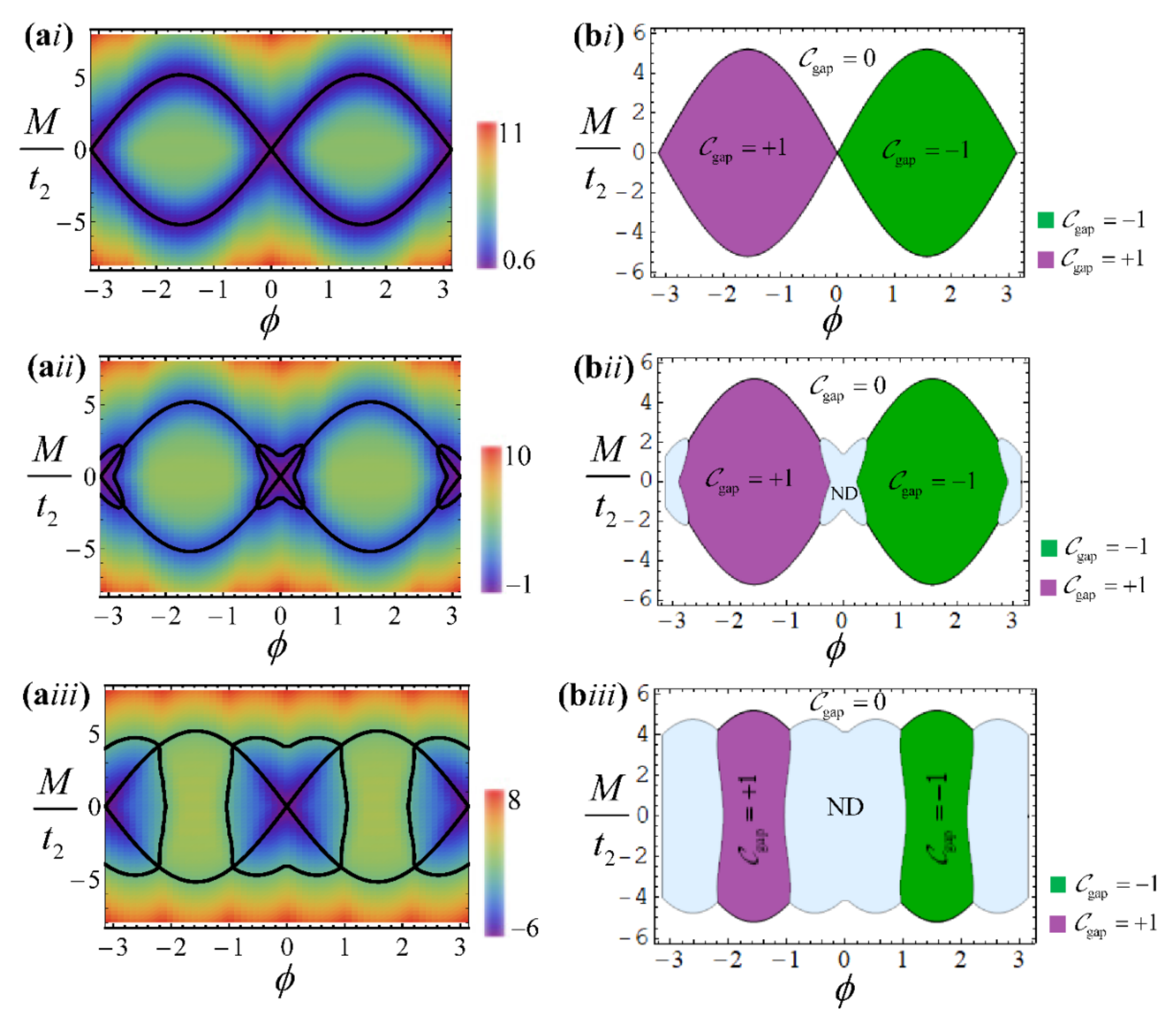
The gap Chern number was numerically determined for different combinations of $\left(\varphi ,M\right)$. In this manner, we recovered the well-known phase diagram represented in Figure 2(bi). As it is well established, the system is characterized by a nontrivial topological phase (${\mathcal{C}}_{\mathrm{gap}}=\pm 1$) when the effects of the broken time-reversal symmetry dominate. Otherwise, when the effects of the broken inversion symmetry dominate (large $\left|M\right|$ parameter) the system is topologically trivial. Note that when $\varphi \ne 0,\pi$ the system has a broken time-reversal symmetry, while when $M\ne 0$, the system has a broken inversion symmetry.

In Figure 2a, we show a density plot of the bandgap width ${\mathcal{E}}_{\mathrm{gap}}$ in between the two energy bands of the Haldane model for different values of $\left(\varphi ,M\right)$. The band-gap width is defined as ${\mathcal{E}}_{\mathrm{gap}}={\min }_{k\in \mathrm{BZ}}{\mathcal{E}}_k^{+}-{\max }_{k\in \mathrm{BZ}}{\mathcal{E}}_k^{-}$, where ${\mathcal{E}}_k^{-}<{\mathcal{E}}_k^{+}$ give the dispersion of the two energy bands. The gap energy ${\mathcal{E}}_{\mathrm{gap}}$ vanishes for the pairs of $\left(\varphi ,M\right)$ where the bandgap closes at the Dirac points corresponding to the black thick lines in Figure 2. Positive values of the ${\mathcal{E}}_{\mathrm{gap}}$ correspond to configurations with a full band-gap, whereas negative values of ${\mathcal{E}}_{\mathrm{gap}}$ correspond to configurations with no band-gap. When ${\mathcal{E}}_{\mathrm{gap}}<0$, the maximum of the low-energy band is larger than the minimum of the high-frequency band. Note that this situation can occur even if the two bands do not intersect and ${\mathcal{E}}_k^{-}<{\mathcal{E}}_k^{+}$ in the entire Brillouin zone. As seen in Figure 2a, it is possible to have configurations with ${\mathcal{E}}_{\mathrm{gap}}<0$ when $\left|t_1\right|/t_2$ is sufficiently small (panels (ii) and (iii)). To our best knowledge, the case ${\mathcal{E}}_{\mathrm{gap}}<0$ was not previously discussed in the literature. Figure 2b shows the numerically calculated topological phase diagram, with the gap Chern number obtained by numerical integration (Equation (13)). Evidently, the Chern number is not defined in the regions with ${\mathcal{E}}_{\mathrm{gap}}<0$ (ND regions). Due to this reason, the diagrams of Figure 2(bii,biii) are different from the standard diagram of Figure 2(bi).

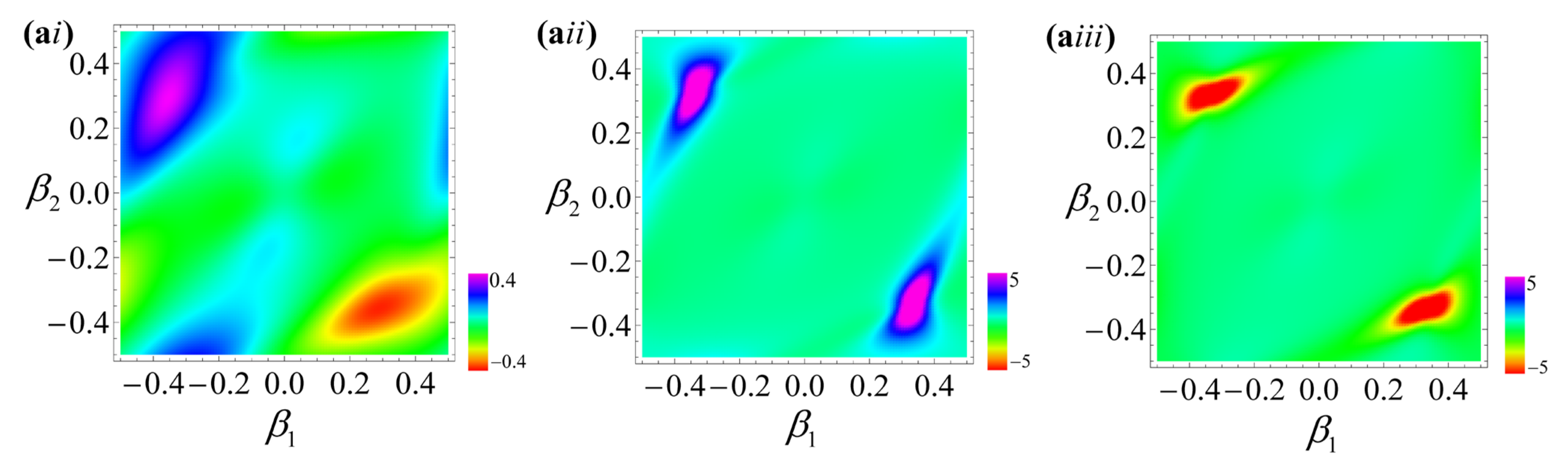
Figure 3 shows the density plots of the Berry curvature numerically calculated with Green’s function theory (Equation (14b)) for different combinations of the $\varphi$ and $M$ parameters. The Brillouin zone is parameterized as $k={\beta }_1{b}_1+{\beta }_2{b}_2$ with $-1/2<{\beta }_i<1/2$. As seen, for the topologically trivial phase with $M/t_2=5$, $\varphi =0$, (Figure 3(ai)), the Berry curvature has both positive and negative values, so that its integral vanishes (Figure 2(bi)). In contrast, for the topologically nontrivial case with $M=0,\varphi \ne 0$, the Berry curvature is either mostly negative with $\varphi =0.2$ (Figure 3(aii)) or positive with $\varphi =-0.2$ (Figure 3(aiii)). The Berry curvature is peaked near the Dirac points. The Berry curvature can change appreciably within the same topological phase but its integral over the Brillouin zone (the gap Chern number) is invariant.

3.2. Topological Phases of the Photonic Haldane Model: Theory

Next, we tackle the more difficult problem of finding the gap Chern number of the photonic Haldane model, without relying on the tight-binding approximation.

To begin with, we rewrite secular Equation (10) as

$$\widehat{L}\left(-i\nabla \right)\cdot E_z=\mathcal{E}{E}_z,$$

(15)

with $\mathcal{E}={\left(\omega /c\right)}^2$ and,

$$\begin{array}{ll}\widehat{L}\left(-i\nabla \right)& =-{\left(\nabla -i\frac{\omega }{c}\widehat{z}\times \xi \left(r\right)\right)}^2+\frac{{\omega }_p^2\left(r\right)}{c^2}\\ & \approx -{\left(\nabla -i\frac{{\omega }_0}{c}\widehat{z}\times \xi \left(r\right)\right)}^2+\frac{{\omega }_p^2\left(r\right)}{c^2}\\ & =-{\nabla }^2+i\frac{{\omega }_0}{c}\left[\nabla \cdot \left(\widehat{z}\times \xi \left(r\right)\right)+\widehat{z}\times \xi \left(r\right)\cdot \nabla \right]+\mathcal{V}\left(r\right)\end{array}$$

(16)

where $\mathcal{V}\left(r\right)=\frac{{\omega }_p^2\left(r\right)}{c^2}+\frac{{\omega }_0^2}{c^2}{\left|\xi \left(r\right)\right|}^2$. In the second identity of the above equation, we replaced $\omega \to {\omega }_0$, where ${\omega }_0$ is some constant frequency. This approximation transforms the secular equation into a standard eigenvalue problem and avoids complications due to material dispersion. Provided that ${\omega }_0$ is some frequency inside the relevant gap of the unperturbed operator, the replacement $\omega \to {\omega }_0$ does not change the physics.

The Bloch modes associated with the wave vector $k=k_x\widehat{x}+k_y\widehat{y}$ are of the form $E_z=e_z\left(x,y\right)e^{ik\cdot r}$, with the envelope $e_z\left(x,y\right)$ being a periodic function that satisfies

$${\widehat{L}}_k\cdot e_z=\mathcal{E}{e}_z, \mathrm{with} {\widehat{L}}_k=\widehat{L}\left(-i\nabla +k\right).$$

(17)

Thus, we obtain a standard eigenvalue problem with a trivial $M_g=1$ operator.

In order to find the spectrum of ${\widehat{L}}_k$ and the topological phases, next we obtain a representation of ${\widehat{L}}_k$ in a plane wave basis [40]. First, we expand the periodic functions $\xi$ and $\mathcal{V}$ into a Fourier series as $\xi ={\displaystyle \sum _J{\xi }_J}{e}^{i{G}_{\mathrm{J}}·\mathrm{r}}$ and $\mathcal{V}={\displaystyle \sum _J{\mathcal{V}}_J}{e}^{i{G}_{\mathrm{J}}·\mathrm{r}}$. Here, $G_J=j_1{b}_1+j_2{b}_2$ and $J=\left(j_1,j_2\right)$ is a pair of integers. From Equation (12), it is readily seen that:

$${\xi }_J={\xi }_0\frac{\sqrt{3}a}{4\pi }\frac{e^{-i{G}_J\cdot r_{\mathrm{c}}}}{2i}\left\{\begin{array}{ll}\pm b_1,& J=\pm \left(1,0\right)\\ \pm b_2,& J=\pm \left(0,1\right)\\ \pm \left(b_1+b_2\right),& J=\pm \left(1,1\right)\\ 0,& \mathrm{otherwise}\end{array}\right..$$

(18)

The Fourier coefficients of the function $g={\omega }_p^2\left(r\right)/c^2$ are $p_{g,I}=\frac{1}{A_{\mathrm{cell}}}{\displaystyle \underset{\mathrm{cell}}{\int }g}\left(r\right)e^{-i{G}_I\cdot r}{d}^{2}r$. A straightforward analysis shows that:

$$p_{g,I}=g_b{\delta }_{I,0}+{\displaystyle \sum _{i=1,2}{f}_{V,i}\left(g_i-g_b\right)e^{-i{G}_I\cdot r_{0,i}}}\frac{2J_1\left(\left|G_I\right|R_i\right)}{\left|G_I\right|R_i},$$

(19)

where ${\delta }_{I,0}$ is Kronecker’s symbol, $J_1$ is the cylindrical Bessel function of the first kind and first order, $R_i$ is the radius of the scattering centers of the i-th array, $r_{0,i}$ gives the position of the i-th scattering center in the unit cell, and $f_{V,i}=\pi R_i^2/A_{\mathrm{cell}}$ with $A_{\mathrm{cell}}=\left|b_1\times b_2\right|$ the area of the unit cell. We use $g_b={\omega }_{p,b}^2/c^2$ and $g_i={\omega }_{p,i}^2/c^2$ (i = 1, 2), with the ${\omega }_{p,i}^{}$ defined as in Figure 1. Finally, from $\mathcal{V}\left(r\right)=\frac{{\omega }_p^2\left(r\right)}{c^2}+\frac{{\omega }_0^2}{c^2}{\left|\xi \left(r\right)\right|}^2$, one finds that the Fourier coefficients of $\mathcal{V}$ are given by:

$${\mathcal{V}}_J=p_{{\omega }_p^2/c^2,J}+\frac{{\omega }_0^2}{c^2}{\displaystyle \sum _{\begin{array}{l}{J}^{\prime }=\pm \left(1,0\right),\\ \pm \left(0,1\right),\pm \left(1,1\right)\end{array}}{\xi }_{J-J^{\prime }}\cdot {\xi }_{J^{\prime }}}.$$

(20)

Here, $p_{{\omega }_p^2/c^2,J}$ is defined as in Equation (19) now with $g={\omega }_p^2/c^2$. Note that the second term can be nonzero only for $\left|j_1\right|\le 2$ and $\left|j_2\right|\le 2$.

We are now ready to obtain a representation of ${\widehat{L}}_k$ in a plane wave basis. To this end, the electric field envelope ($e_z=E_z{e}^{-ik\cdot r}$) is expanded into plane waves as $e_z={\displaystyle \sum _J{c}_J^E{e}^{i{G}_J\cdot r}}$. Then, it is simple to check that Equation (17) implies that for a generic double index $I=\left(i_1,i_2\right)$ one has:

$$\begin{array}{l}\left(k+G_I\right)\cdot \left(k+G_I\right)c_I^E+{\displaystyle \sum _J{\mathcal{V}}_{I-J}{c}_J^E}\\ -\frac{{\omega }_0}{c}{\displaystyle \sum _J\left[\left(k+G_I\right)\cdot \left(\widehat{z}\times {\xi }_{I-J}\right)+\left(\widehat{z}\times {\xi }_{I-J}\right)\cdot \left(k+G_J\right)\right]c_J^E}=\mathcal{E}{c}_I^E\end{array}$$

(21)

From here it is evident that the operator ${\widehat{L}}_k$ is represented by the matrix ${\widehat{L}}_k\to \left[L_{I,J}\right]$ with

$$L_{I,J}=\left(k+G_I\right)\cdot \left(k+G_I\right){\delta }_{I,J}+{\mathcal{V}}_{I-J}-\frac{{\omega }_0}{c}\left[\left(k+G_I\right)\cdot \left(\widehat{z}\times {\xi }_{I-J}\right)+\left(\widehat{z}\times {\xi }_{I-J}\right)\cdot \left(k+G_J\right)\right].$$

(22)

The operators ${\partial }_i{\widehat{L}}_k$ are represented by matrices with generic elements

$${\left[{\partial }_i{\widehat{L}}_k\right]}_{I,J}=2{\widehat{u}}_i\cdot \left(k+G_I\right){\delta }_{I,J}-\frac{{\omega }_0}{c}\left(2{\widehat{u}}_i\cdot \left(\widehat{z}\times {\xi }_{I-J}\right)\right),$$

(23)

where ${\widehat{u}}_1=\widehat{x}$ and ${\widehat{u}}_2=\widehat{y}$ are unit vectors along the coordinates axes. In the numerical calculations the plane wave expansion is truncated imposing that $J=\left(j_1,j_2\right)$ with $\left|j_m\right|\le j_{\max }$ with m = 1,2. To conclude, we note that the spectral problem (Equation (17)) is equivalent to the matrix eigensystem $\left[L_{I,J}\right]\cdot \left[c_J^E\right]=\mathcal{E}\left[c_J^E\right]$.

3.3. Topological Phases of the Photonic Haldane Model: Numerical Results

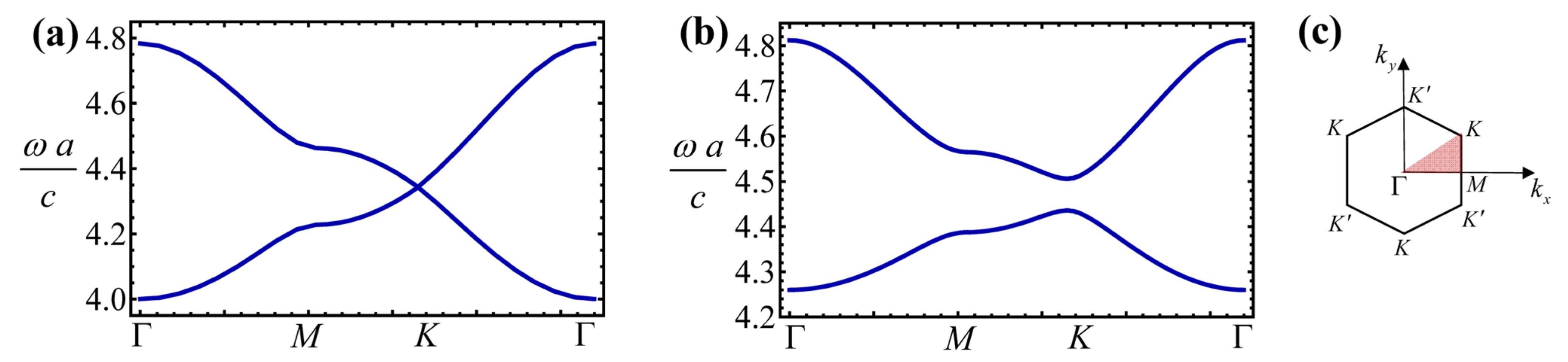
The band structures of two Haldane photonic crystals are plotted in Figure 4. The scattering centers have a trivial electric response (${\omega }_{p,1}={\omega }_{p,2}=0$), whereas the background region is characterized by the plasma frequency ${\omega }_{p,b}\hspace{0.17em}a/c=5.63$. In the numerical simulations, the plane wave expansion was truncated with $j_{\max }=3$.

The reciprocal case characterized by ${\xi }_0=0$ is shown in Figure 4a, and corresponds to a photonic analogue of graphene [22]. Due to the plasmonic response of the host medium there is a bandgap for low frequencies ($\omega a/c<4.25$). The nonreciprocal crystal in Figure 4b is characterized by a nontrivial spatially dependent pseudo-Tellegen response with a peak amplitude ${\xi }_0=0.677$.

As seen in Figure 4a, for the reciprocal case, the first two bands touch at the Dirac points (K) due the symmetry of the hexagonal lattice (${\omega }_{p,1}={\omega }_{p,2}$). On the other hand, when the pseudo-magnetic field associated with the Tellegen coupling is nontrivial (${\xi }_0\ne 0$) the degeneracy around the Dirac points is lifted, leading to the separation of the bands and to a complete photonic band-gap. Thus, analogous to the electronic Haldane model [2], the time-reversal symmetry breaking opens a gap between the first and the second bands of the system (Figure 4).

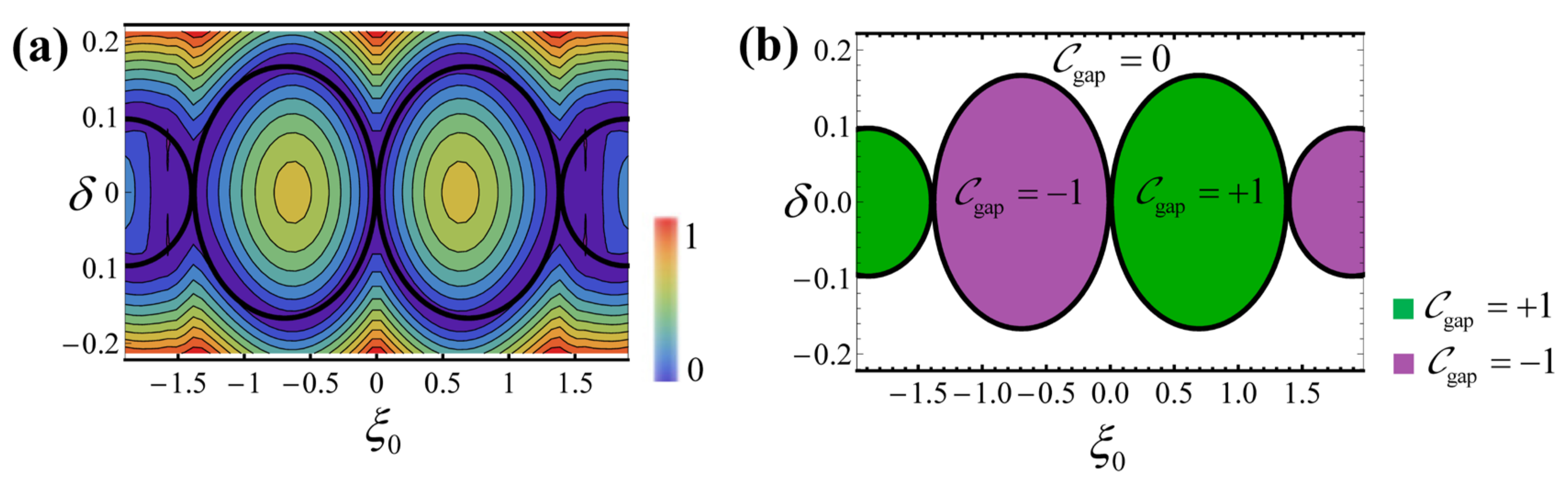
The phase diagram of the Tellegen photonic crystals is plotted in Figure 5. To model the structural asymmetry between the two sub-lattices of the hexagonal array, we introduce a spatial-asymmetry parameter $\delta$ such that for $\delta >0$ the plasma frequencies of the scattering centers satisfy ${\omega }_{p,1}=\delta \times {\omega }_{p,b}$ and ${\omega }_{p,2}=0$, whereas for $\delta <0$ they satisfy ${\omega }_{p,1}=0$ and ${\omega }_{p,2}=\left|\delta \right|\times {\omega }_{p,b}$. For $\delta \ne 0$ the inversion symmetry of the system is broken. In Figure 5a, we show a density plot of the band-gap “energy” ${\mathcal{E}}_{\mathrm{gap}}$ for different pairs of $\left({\xi }_0,\delta \right)$. As seen, for the photonic crystal implementation of the Haldane model ${\mathcal{E}}_{\mathrm{gap}}\ge 0$, and so that the topological characterization is feasible in the entire parameter space. The black thick lines represent the combinations of $\left({\xi }_0,\delta \right)$ for which the bandgap closes.

The topological phase diagram of the Tellegen photonic crystal is shown in Figure 5b. The gap Chern number is calculated from first principles using Green’s function theory. The different topological phases are shaded with different colors and the corresponding gap Chern numbers are identified inside the curves. As seen, analogous to the tight-binding model, when the time-reversal symmetry breaking dominates (large values of $\left|{\xi }_0\right|$), the photonic crystal is topologically nontrivial and the gap Chern number is ${\mathcal{C}}_{\mathrm{gap}}=\pm 1$. In contrast, when the inversion symmetry breaking dominates (large values of $\left|\delta \right|$), the system is topologically trivial.

Curiously, the topological charge depends not only on the sign of ${\xi }_0$, but also on its amplitude. For example, for $0<{\xi }_0<1.36$ the gap Chern number is +1, but for values of ${\xi }_0$ slightly larger than 1.36, the sign of the gap Chern number changes due to a phase transition. As a consequence, the topological phase diagram is formed by a sequence of bubble-type regions with alternating sign of the gap Chern number. This example illustrates the richness of topological phenomena in photonic crystals, which arises due to periodicity and granular nature of the system, and which can only be captured with a “first principles” approach. It is relevant to note that $\left({\xi }_0,\delta \right)$ can be mapped into the parameters $\left(\varphi ,M\right)$ of the equivalent tight-binding model (Equation (1)), see [21]. Comparing Figure 2b and Figure 5b, one sees that, for a sufficiently small $\left|{\xi }_0\right|$, the sign of the equivalent $\varphi$ is opposite to the sign of ${\xi }_0$ [21,22].

4. Summary

In this article, we determined the topological phases of a photonic analogue of the Haldane model using a first-principles Green’s function approach. The proposed system consists of a hexagonal array of dielectric cylinders embedded in a metallic host, with a spatially varying pseudo-Tellegen coupling playing the role a pseudo-magnetic field. The Tellegen nonreciprocal response is at the origin of the nontrivial topology of the photonic crystal. Interestingly, the results of the first principles calculations show that even though a bulk pseudo-Tellegen medium has a trivial topology, a nonuniform pseudo-Tellegen structure (photonic crystal) can have topological bandgaps. Furthermore, it was found that due to the complex wave interactions arising from the scattering by the potential-well centers, the phase diagram of the photonic crystal can have nontrivial features and a bubble-type structure different from what is predicted by Haldane’s tight-binding model. We expect that Green’s function method can find many other applications in the characterization of the topology of emerging photonic systems.

References

- Thouless, D.J.; Kohmoto, M.; Nightingale, M.P.; den Nijs, M. Quantized Hall conductance in a two-dimensional periodic potential. Phys. Rev. Lett. 1982, 49, 405. [Google Scholar] [CrossRef] [Green Version]
- Haldane, F.D.M. Model for a quantum Hall effect without Landau levels: Condensed-matter realization of the “parity anomaly”. Phys. Rev. Lett. 1988, 61, 2015–2018. [Google Scholar] [CrossRef]
- Hasan, M.Z.; Kane, C.L. Colloquium: Topological insulators. Rev. Mod. Phys. 2010, 82, 3045–3067. [Google Scholar] [CrossRef] [Green Version]
- Haldane, F.D.M. Nobel lecture: Topological quantum matter. Rev. Mod. Phys. 2017, 89, 040502. [Google Scholar] [CrossRef]
- Lu, L.; Joannopoulos, J.D.; Soljacic, M. Topological photonics. Nat. Photonics 2014, 8, 821. [Google Scholar] [CrossRef] [Green Version]
- Ozawa, T.; Price, H.M.; Amo, A.; Goldman, N.; Hafezi, M.; Lu, L.; Rechtsman, M.C.; Schuster, D.; Simon, J.; Zilberberg, O.; et al. Topological photonics. Rev. Mod. Phys. 2019, 91, 015006. [Google Scholar] [CrossRef] [Green Version]
- Haldane, F.D.M.; Raghu, S. Possible realization of directional optical waveguides in photonic crystals with broken time-reversal symmetry. Phys. Rev. Lett. 2008, 100, 013904. [Google Scholar] [CrossRef] [Green Version]
- Raghu, S.; Haldane, F.D.M. Analogs of quantum-Hall-effect edge states in photonic crystals. Phys. Rev. A 2008, 78, 033834. [Google Scholar] [CrossRef] [Green Version]
- Wang, Z.; Chong, Y.; Joannopoulos, J.D.; Soljačić, M. Observation of unidirectional backscattering-immune topological electromagnetic states. Nat. Cell Biol. 2009, 461, 772–775. [Google Scholar] [CrossRef] [Green Version]
- Khanikaev, A.B.; Mousavi, S.H.; Tse, W.K.; Kargarian, M.; MacDonald, A.H.; Shvets, G. Photonic topological insulators. Nat. Mater. 2012, 12, 233. [Google Scholar] [CrossRef]
- Rechtsman, M.C.; Zeuner, J.M.; Plotnik, Y.; Lumer, Y.; Podolsky, D.; Dreisow, F.; Nolte, S.; Segev, M.; Szameit, A. Photonic Floquet topological insulators. Nat. Cell Biol. 2013, 496, 196–200. [Google Scholar] [CrossRef]
- Silveirinha, M.G. Chern invariants for continuous media. Phys. Rev. B 2015, 92, 125153. [Google Scholar] [CrossRef]
- Silveirinha, M.G. Bulk-edge correspondence for topological photonic continua. Phys. Rev. B 2016, 94, 205105. [Google Scholar] [CrossRef] [Green Version]
- Silveirinha, M.G. Quantized angular momentum in topological optical systems. Nat. Commun. 2019, 10, 349. [Google Scholar] [CrossRef]
- Silveirinha, M.G. Proof of the bulk-edge correspondence through a link between topological photonics and fluctuation-electrodynamics. Phys. Rev. 2019, 9, 011037. [Google Scholar] [CrossRef] [Green Version]
- Leykam, D.; Bliokh, K.; Huang, C.; Chong, Y.; Nori, F. Edge modes, degeneracies, and topological numbers in non-Hermitian systems. Phys. Rev. Lett. 2017, 118, 040401. [Google Scholar] [CrossRef] [Green Version]
- Shen, H.; Zhen, B.; Fu, L. Topological band theory for non-Hermitian Hamiltonians. Phys. Rev. Lett. 2018, 120, 146402. [Google Scholar] [CrossRef] [Green Version]
- Yao, S.; Wang, Z. Edge states and topological invariants of non-Hermitian systems. Phys. Rev. Lett. 2018, 121, 086803. [Google Scholar] [CrossRef] [PubMed] [Green Version]
- Silveirinha, M.G. Topological theory of non-Hermitian photonic systems. Phys. Rev. B 2019, 99, 125155. [Google Scholar] [CrossRef] [Green Version]
- Lannebère, S.; Silveirinha, M.G. Effective Hamiltonian for electron waves in artificial graphene: A first principles derivation. Phys. Rev. B 2015, 91, 045416. [Google Scholar] [CrossRef] [Green Version]
- Lannebère, S.; Silveirinha, M.G. Link between the photonic and electronic topological phases in artificial graphene. Phys. Rev. B 2018, 97, 165128. [Google Scholar] [CrossRef] [Green Version]
- Lannebère, S.; Silveirinha, M.G. Photonic analogues of the Haldane and Kane-Mele models. Nanophotonics 2019, 8, 1387–1397. [Google Scholar] [CrossRef]
- Silveirinha, M.G. Topological classification of Chern-type insulators by means of the photonic Green function. Phys. Rev. B 2018, 97, 115146. [Google Scholar] [CrossRef] [Green Version]
- Prudêncio, F.R.; Silveirinha, M.G. First principles calculation of topological invariants of non-Hermitian photonic crystals. Comm. Phys. 2020, 3, 221. [Google Scholar] [CrossRef]
- Bernevig, B.A.; Hughes, T.L. Topological Insulators and Topological Superconductors; Princeton University Press: Oxford, UK, 2013. [Google Scholar]
- Jacobs, D.A.; Miroshnichenko, A.E.; Kivshar, Y.S.; Khanikaev, A.B. Photonic topological Chern insulators based on Tellegen metacrystals. New J. Phys. 2015, 17, 125015. [Google Scholar] [CrossRef] [Green Version]
- Serdyukov, A.; Semchenko, I.; Tretyakov, S.; Sihvola, A. Electromagnetics of Bi-Anisotropic Materials: Theory and Applications; Gordon and Breach Science Publishers: Amsterdam, The Netherlands, 2001. [Google Scholar]
- Astrov, D.N. Magnetoelectric effect in chromium oxide. Sov. Phys. JETP 1961, 13, 729. [Google Scholar]
- Qi, X.L.; Li, R.; Zang, J.; Zhang, S.C. Inducing a magnetic monopole with topological surface states. Science 2009, 323, 1184–1187. [Google Scholar] [CrossRef] [Green Version]
- Qi, X.L.; Zhang, S.C. Topological insulators and superconductors. Rev. Mod. Phys. 2011, 83, 1057. [Google Scholar] [CrossRef] [Green Version]
- Coh, S.; Vanderbilt, D. Canonical magnetic insulators with isotropic magnetoelectric coupling. Phys. Rev. B 2013, 88, 121106. [Google Scholar] [CrossRef] [Green Version]
- Mong, R.S.K.; Essin, A.M.; Moore, J.E. Antiferromagnetic topological insulators. Phys. Rev. B 2010, 81, 245209. [Google Scholar] [CrossRef] [Green Version]
- Dziom, V.; Shuvaev, A.; Pimenov, A.; Astakhov, G.V.; Ames, C.; Bendias, K.; Böttcher, J.; Tkachov, G.; Hankiewicz, E.M.; Brüne, C.; et al. Observation of the universal magnetoelectric effect in a 3D topological insulator. Nat. Commun. 2017, 8, 15197. [Google Scholar] [CrossRef] [PubMed] [Green Version]
- Prudencio, F.; Matos, S.; Paiva, C.R. Exact image method for radiation problems in stratified isorefractive Tellegen media. IEEE Trans. Antennas Propag. 2014, 62, 4637–4646. [Google Scholar] [CrossRef]
- Prudencio, F.R.; Matos, S.A.; Paiva, C.R. A geometrical approach to duality transformations for Tellegen media. IEEE Trans. Microw. Theory Tech. 2014, 62, 1417–1428. [Google Scholar] [CrossRef]
- Prudêncio, F.R.; Matos, S.A.; Paiva, C.R. Asymmetric band diagrams in photonic crystals with a spontaneous nonreciprocal response. Phys. Rev. A 2015, 91, 063821. [Google Scholar] [CrossRef] [Green Version]
- Prudêncio, F.R.; Silveirinha, M.G. Optical isolation of circularly polarized light with a spontaneous magnetoelectric effect. Phys. Rev. A 2016, 93, 043846. [Google Scholar] [CrossRef]
- Zhao, R.; Xie, G.-D.; Chen, M.L.N.; Lan, Z.; Huang, Z.; Sha, W.E.I. First-principle calculation of Chern number in gyrotropic photonic crystals. Opt. Express 2020, 28, 4638–4649. [Google Scholar] [CrossRef] [PubMed] [Green Version]
- Chen, M.L.N.; Jiang, L.J.; Zhang, S.; Zhao, R.; Lan, Z.; Sha, W.E.I. Comparative study of Hermitian and non-Hermitian topological dielectric photonic crystals. Phys. Rev. A 2021, 104, 033501. [Google Scholar] [CrossRef]
- Sakoda, K. Optical Properties of Photonic Crystals; Springer: Berlin, Germany, 2001. [Google Scholar]
Figure 1.
Illustrative geometry of (a) the electronic Haldane model and (b) the equivalent photonic structure. (a) Representation of the lines of the periodic vector potential (black arrows). The disks indicate the location of the scattering centers associated with the electrostatic potentials (i = 1, 2). In the background region, the potential is . The distance between nearest neighbors is a. (b) Representation of the lines of the pseudo-Tellegen vector (black arrows) that determines the nonreciprocal coupling. The plasma frequencies in the scattering centers and in the background are (i = 1, 2) and , respectively.
Figure 2.
(a) Density plot of the band-gap energy for different combinations of the phase and mass parameters , for (i) , (ii) , and (iii) . The thick black lines correspond to the pairs where the band-gap closes. Negative values of the band-gap energy represent configurations for which there is no band-gap. (b) Numerically calculated topological phase diagram for the same configurations as in (a). The gap Chern number is determined through Equation (13). The different topological phases are shaded with different colors. The ND (non-defined) region corresponds to the pairs for which there is no gap, and thereby the topological number is not defined.
Figure 3.
Density plot of the Berry curvature of the band below the gap, (Equation (14b)) in the first Brillouin zone for . The parameters of the Haldane model are (ai) and . (aii) and . (aiii) and .
Figure 4.
(a,b) Band structure of the Haldane photonic crystal. The plasma frequencies of the scatterers are ; the plasma frequency of the background material is . The radius of the two scatterers is . (a) Reciprocal system with . (b) Nonreciprocal system with and . (c) Sketch of the first Brillouin zone of the hexagonal lattice.
Figure 5.
(a) Density plot of the band-gap “energy” for different combinations of the peak amplitude of the pseudo-Tellegen vector and of spatial-asymmetry parameters . The thick black lines correspond to the pairs of for which the band-gap closes. (b) Topological phase diagram of the photonic Haldane photonic crystal. The different topological phases are shaded with different colors. The remaining parameters are as in Figure 4.
Publisher’s Note: MDPI stays neutral with regard to jurisdictional claims in published maps and institutional affiliations. |
© 2021 by the authors. Licensee MDPI, Basel, Switzerland. This article is an open access article distributed under the terms and conditions of the Creative Commons Attribution (CC BY) license (https://creativecommons.org/licenses/by/4.0/).
Share and Cite
MDPI and ACS Style
Prudêncio, F.R.; Silveirinha, M.G. First Principles Calculation of the Topological Phases of the Photonic Haldane Model. Symmetry 2021, 13, 2229. https://0-doi-org.brum.beds.ac.uk/10.3390/sym13112229
AMA Style
Prudêncio FR, Silveirinha MG. First Principles Calculation of the Topological Phases of the Photonic Haldane Model. Symmetry. 2021; 13(11):2229. https://0-doi-org.brum.beds.ac.uk/10.3390/sym13112229
Chicago/Turabian StylePrudêncio, Filipa R., and Mário G. Silveirinha. 2021. "First Principles Calculation of the Topological Phases of the Photonic Haldane Model" Symmetry 13, no. 11: 2229. https://0-doi-org.brum.beds.ac.uk/10.3390/sym13112229
Note that from the first issue of 2016, this journal uses article numbers instead of page numbers. See further details here.