Periodicity on Neutral-Type Inertial Neural Networks Incorporating Multiple Delays

Abstract

The classical Hopefield neural networks have obvious symmetry, thus the study related to its dynamic behaviors has been widely concerned. This research article is involved with the neutral-type inertial neural networks incorporating multiple delays. By making an appropriate Lyapunov functional, one novel sufficient stability criterion for the existence and global exponential stability of T-periodic solutions on the proposed system is obtained. In addition, an instructive numerical example is arranged to support the present approach. The obtained results broaden the application range of neutral-types inertial neural networks.

1. Introduction

The well-known inertial neural networks (INNs) were first introduced by Babcock and Westervelt [1,2], and can be expressed as the following functional differential equations:

$$s_j^{\prime \prime }\left(t\right)=-a_j{s}_j^{\prime }\left(t\right)-b_j{s}_j\left(t\right)+\sum _{k=1}^n{c}_{jk}{f}_k\left(s_k\left(t\right)\right)+\sum _{k=1}^n{d}_{jk}{f}_k\left(s_k\left(t-{\tau }_{jk}\right)\right)+I_j,t\ge 0,$$

(1)

with the initial value conditions:

$$s_j\left(v\right)={\phi }_j\left(v\right),s_j^{\prime }\left(0\right)={\psi }_j,-{\tau }_j^{+}\le vs.\le 0,{\phi }_j\in C([-{\tau }_j^{+},0],\mathbb{R}),{\psi }_j\in \mathbb{R},$$

(2)

where ${\tau }_j^{+}=\underset{1\le k\le n}{max}\left\{{\tau }_{jk}\right\}$, $s\left(t\right)=(s_1\left(t\right),s_2\left(t\right),\dots ,s_n\left(t\right))$ represents the state vector, $s_j^{\prime \prime }\left(t\right)$ is referred to an inertial item of the j-th neuron on (1), the parameters $a_j>0,b_j>0,c_{jk},d_{jk}$ and time delay ${\tau }_{jk}\ge 0$ are real numbers, $I_j$ is the external input, $f_k$ is a continuous activation function, $j,k\in \mathfrak{N}:=\{1,2,\dots ,n\}.$

During the past thirty decades, by utilizing the reduced-order transformation, numerous studies have been conducted on the stability and synchronization of system (1) and its generalizations, such as [3,4,5,6,7,8,9,10,11]. However, the reduced-order method will affect the dimensions of systems, thereby increasing a large amount of calculation, which will make it difficult to achieve in practice. For the sake of avoiding the traditional reduced-order method, the authors proposed several new criteria for the stability and synchronization of the system (1) in [12,13] through making a new Lyapunov functional. On this basis, references [14,15,16,17,18,19,20,21] extensively studied various dynamic behaviors of system (1) and its generalizations via applying the non-reduced order approach.

It is well known that the classical Hopefield neural networks have obvious symmetry, numerous researchers have carried out extensive research on its related dynamic behaviors [16,22,23,24]. In particular, the authors in [25] investigate the exponential stability and the almost sure exponential stability for a class of stochastic fuzzy Cohen-Grossberg neural networks by fabricating an appropriate Lyapunov functional. In practical application, owing to the finite switching and transmission speeds of signals in the networks, the existence of time delays is inevitable in the working networks. It should be pointed out that in addition to the state itself, there are also time delays in the derivatives of the state related to the networks. This kind of delay is deemed as neutral delay, which not only appears in the field of automatic control and population ecology [26,27], but also occurs in many physical systems, including transmission lines, Lotka–Volterra systems, chemical reactors, and others [23,24,28,29]. Particularly, if we use differential equations to model neural networks (NNs) for the realization of electronic circuits, the influence of neutral delay often exists. The authors in [24,29] investigated the effect of neutral delays on the partial element equivalent circuit. The circuit was represented to a neutral-type functional differential equation, and some new sufficient stability assertions were given by Lyapunov theory. Furthermore, the dynamic behaviors of neutral-type inertial neural networks (NTINNs) have been extensively studied by exploiting the reduced-order approach. For example, the authors in [30] used the finite-time stability theory, inequality techniques and analysis approaches to research the finite-time synchronization on fuzzy NTINNs. In [31], the stability of NTINNs is studied via utilizing the Lyapunov–Krasovskii functional approach and Linear Matrix Inequality (LMI) analysis.

On the other hand, periodic phenomena are widespread in biological systems. For instance, seasonal influences of weather and food supplies, electronic systems, NNs etc. Especially in the application of NNs, periodic phenomenon is one of the most important dynamic behaviors to describe the symmetry of the Hopefield neural networks model, and the existence and stability of periodic solutions will help us to understand the asymptotic behavior of mathematical biological systems. Therefore, it is a very meaningful thing to research the existence and stability of periodic solutions [24,32]. However, few researches have discussed the periodic problem of the following NTINNs involving multiple delays:

$$\begin{array}{ccc}\hfill s_j^{\prime \prime }\left(t\right)-\sum _{k=1}^n{e}_{jk}{s}_k^{\prime \prime }(t-{\xi }_{jk})& =& -a_j{s}_j^{\prime }\left(t\right)-b_j{s}_j\left(t\right)+\sum _{k=1}^n{c}_{jk}{f}_k\left(s_k\left(t\right)\right)\hfill \\ & & +\sum _{k=1}^n{d}_{jk}{f}_k\left(s_k(t-{\tau }_{jk})\right)+I_j\left(t\right),t\ge 0,\hfill \end{array}$$

(3)

with the initial conditions:

$$s_j\left(v\right)={\phi }_j\left(v\right),s_j^{\prime }\left(v\right)={\psi }_j\left(v\right),s_j^{\prime \prime }\left(v\right)={\varsigma }_j\left(v\right),-{\sigma }_j\le vs.\le 0,{\phi }_j,{\psi }_j,{\varsigma }_j\in C\left([-{\sigma }_j,0],\mathbb{R}\right),$$

(4)

where ${\xi }_j^{+}=\underset{1\le k\le n}{max}\left\{{\xi }_{jk}\right\},{\sigma }_j=max\{{\tau }_j^{+},{\xi }_j^{+}\},$$e_{jk}$ and the multiple neutral delays ${\xi }_{jk}\ge 0$ are constants, $I_j\left(t\right)$ is a continuous periodic function involving period $T>0$, and $j,k\in \mathfrak{N}$.

Enlightened by the above arguments, our major purpose in this article is to investigate the existence and stability of periodic solutions on NTINNs involving multiple delays through constructing a new and appropriate Lyapunov functional to replace the traditional reduced-order approach. Briefly speaking, the innovative contents of this article can be presented as below. (1) A class of NTINNs involving multiple delays is proposed; (2) Under certain assumptions, by exploiting the non-reduced order approach, one new sufficient stability criterion to guarantee the existence and stability of the T-periodic solutions on system (3) is gotten for the first time; (3) NTINNs here are second-order and involve multiple neutral delays, which are different from the traditional NNs [33,34,35,36,37,38,39,40] or INNs [3,4,5,6,7,8,9,11,12,13,14,15,17,18,19,20,21,30,31,32]. Compared with the results on exponential stability for the neutral-type neural networks (NTNNs) [26,29,39,41] and INNs [13,14,18,19], we give the exponential stability of the T-periodic solution for the NTINNs. (4) An instructive numerical simulation including comparisons is afforded to demonstrate the obtained theoretical results.

This article is systematized as below. In Section 2, a few indispensable lemmas, definitions and assumptions are given. In Section 3, the global exponential stability on the T-periodic solutions of the NTINNs (3) is proved. In Section 4, an instructive numerical simulation is afforded to evidence the validity and feasibility of the analytical results. A concise conclusion is offered in Section 5.

2. Preliminaries

Throughout this article, a few indispensable lemmas, definitions and assumptions are provided, which are useful in the following proving process.

Assumption 1.

There is a nonnegative real number $L_j$ obeying

$$\left|f_j\left(p\right)-f_j\left(q\right)\right|\le L_j|p-q|,\mathit{for}\mathit{all}p,q\in \mathbb{R}\mathit{and}j\in \mathfrak{N}.$$

Assumption 2.

For $j\in \mathfrak{N}$, there remain three real numbers ${\overline{\delta }}_j\ge 0,$ ${\overline{\beta }}_j\ge 0$ and ${\overline{\alpha }}_j>0$ agreeing with that

$${\mathcal{X}}_j<0,4{\mathcal{Y}}_j{\mathcal{X}}_j>{\mathcal{Z}}_j^2,$$

(5)

where

$$\begin{array}{cc}\hfill {\mathcal{X}}_j=& \sum _{k=1}^n\left({\overline{\delta }}_j+{\overline{\beta }}_j^2\right)|e_{jk}|+2{\overline{\alpha }}_j{\overline{\beta }}_j+\sum _{k=1}^n{\overline{\alpha }}_j{\overline{\beta }}_j|e_{jk}|-2a_j{\overline{\alpha }}_j^2+\sum _{k=1}^n{\overline{\alpha }}_j^2|c_{jk}|+\sum _{k=1}^n{\overline{\alpha }}_j^2|d_{jk}|\hfill \\ \hfill & +\sum _{k=1}^n{a}_j{\overline{\alpha }}_j^2|e_{jk}|+\sum _{k=1}^n{a}_j{\overline{\alpha }}_j{\overline{\beta }}_j|e_{jk}|+\sum _{k=1}^n{B}_{kj}^1+\sum _{k=1}^n\sum _{l=1}^n{\tilde{B}}_{kjl}^1,\hfill \\ \hfill {\mathcal{Y}}_j=& \sum _{k=1}^n({\overline{\delta }}_j+{\overline{\beta }}_j^2)|e_{jk}|+\sum _{k=1}^n{b}_j{\overline{\alpha }}_j^2|e_{jk}|-2b_j{\overline{\alpha }}_j{\overline{\beta }}_j+\sum _{k=1}^n{\overline{\alpha }}_j{\overline{\beta }}_j|c_{jk}|+\sum _{k=1}^n{\overline{\alpha }}_j{\overline{\beta }}_j|d_{jk}|\hfill \\ \hfill & +\sum _{k=1}^n{b}_j{\overline{\alpha }}_j{\overline{\beta }}_j|e_{jk}|+(\sum _{k=1}^n{\overline{\alpha }}_k^2|c_{kj}|+\sum _{k=1}^n\sum _{l=1}^n{\overline{\alpha }}_l^2|e_{lk}||e_{lj}|+\sum _{k=1}^n{\overline{\alpha }}_k{\overline{\beta }}_k|c_{kj}|\hfill \\ \hfill & +\sum _{k=1}^n\sum _{l=1}^n{\overline{\alpha }}_l{\overline{\beta }}_l|e_{lk}||c_{lj}|)L_j^2+\sum _{k=1}^n{A}_{kj}^1+\sum _{k=1}^n\sum _{l=1}^n{\tilde{A}}_{kjl}^1+(\sum _{k=1}^n{C}_{kj}+\sum _{k=1}^n\sum _{l=1}^n{\tilde{C}}_{kjl})L_j^2,\hfill \\ \hfill {\mathcal{Z}}_j=& 2({\overline{\delta }}_j+{\overline{\beta }}_j^2)-2b_j{\overline{\alpha }}_j^2-2a_j{\overline{\alpha }}_j{\overline{\beta }}_j,\hfill \end{array}$$

and

$$\begin{array}{cc}\hfill A_{kj}^1& =[{\overline{\delta }}_k+{\overline{\beta }}_k^2+(a_k+b_k){\overline{\alpha }}_k{\overline{\beta }}_k]|e_{kj}|,{\tilde{A}}_{kjl}^1={\overline{\alpha }}_k{\overline{\beta }}_k(|c_{kl}|+|d_{kl}|)|e_{kj}|,\hfill \\ \hfill B_{kj}^1& =\left({\overline{\delta }}_k+{\overline{\beta }}_k^2+2{\overline{\alpha }}_k{\overline{\beta }}_k+a_k{\overline{\alpha }}_k^2+b_k{\overline{\alpha }}_k^2\right)|e_{kj}|,\hfill \\ \hfill {\tilde{B}}_{kjl}^1& =(({\overline{\delta }}_k+{\overline{\beta }}_k^2+2{\overline{\alpha }}_k{\overline{\beta }}_k)|e_{kl}|+{\overline{\alpha }}_k^2(|c_{kl}|+|d_{kl}|))|e_{kj}|,\hfill \\ \hfill C_{kj}& =({\overline{\alpha }}_k^2+{\overline{\alpha }}_k{\overline{\beta }}_k)|d_{kj}|,{\tilde{C}}_{kjl}=({\overline{\alpha }}_k+{\overline{\beta }}_k){\overline{\alpha }}_k|e_{kl}||d_{kj}|,j,k,l\in \mathfrak{N}.\hfill \end{array}$$

Definition 1.

Given $x\left(t\right)= \left(x_1\left(t\right),x_2\left(t\right),\dots ,x_n\left(t\right)\right)$ and $y\left(t\right)=\left(y_1\left(t\right),y_2\left(t\right),\dots ,y_n\left(t\right)\right)$ as two solutions of the NTINNs (3) to satisfy

$$\begin{array}{cc}\hfill x_j\left(v\right)& ={\phi }_j^x\left(v\right),x_j^{\prime }\left(v\right)={\psi }_j^x\left(v\right),x_j^{\prime \prime }\left(v\right)={\varsigma }_j^x\left(v\right),\hfill \\ \hfill y_j\left(v\right)& ={\phi }_j^y\left(v\right),y_j^{\prime }\left(v\right)={\psi }_j^y\left(v\right),y_j^{\prime \prime }\left(v\right)={\varsigma }_j^y\left(v\right),j\in \mathfrak{N},\hfill \end{array}$$

(6)

where ${\phi }_j^x,{\psi }_j^x,{\varsigma }_j^x,{\phi }_j^y,{\psi }_j^y,{\varsigma }_j^y\in C([-{\sigma }_j,0],\mathbb{R}).$ The NTINNs (1.3) is said to have global exponential stability when there are constants $\lambda >0$ and $\Lambda =\Lambda \left({\phi }^x,{\psi }^x,{\varsigma }^x,{\phi }^y,{\psi }^y,{\varsigma }^y\right)>0$ obeying that

$$\left|x_j\left(t\right)-y_j\left(t\right)\right|\le \Lambda e^{-\lambda t},\left|x_j^{\prime }\left(t\right)-y_j^{\prime }\left(t\right)\right|\le \Lambda e^{-\lambda t},forallt\in [0,+\infty )\mathit{and}j\in \mathfrak{N}.$$

Lemma 1.

Under the Assumptions 1 and 2, every solution of NTINNs (3) incorporating initial values (4) exists and is unique on $[0,+\infty )$.

Proof. 

At first, set

$$\iota =\underset{1\le j\le n}{min}\left\{{\tau }_j^{-},{\xi }_j^{-}\right\},w_j\left(t\right)=s_j\left(t\right)-\sum _{k=1}^n{e}_{jk}{s}_k(t-{\xi }_{jk}),$$

where ${\tau }_j^{-}=\underset{1\le k\le n}{min}\left\{{\tau }_{jk}\right\},{\xi }_j^{-}=\underset{1\le k\le n}{min}\left\{{\xi }_{jk}\right\}\mathit{and}j\in \mathfrak{N}.$ Now, we prove that $s_j\left(t\right)$ exists and is unique on $[0,\iota ].$ Actually, for all $t\in [0,\iota ]$ and $j\in \mathfrak{N}$,

$$\begin{array}{cc}\hfill w_j^{\prime \prime }\left(t\right)=& s_j^{\prime \prime }\left(t\right)-\sum _{k=1}^n{e}_{jk}{s}_k^{\prime \prime }\left(t-{\xi }_{jk}\right)\hfill \\ \hfill =& -a_j{s}_j^{\prime }\left(t\right)-b_j{s}_j\left(t\right)+\sum _{k=1}^n{c}_{jk}{f}_k\left(s_k\left(t\right)\right)+\sum _{k=1}^n{d}_{jk}{f}_k\left(s_k\left(t-{\tau }_{jk}\right)\right)+I_j\left(t\right)\hfill \\ \hfill =& -a_j{w}_j^{\prime }\left(t\right)-b_j{w}_j\left(t\right)-a_j\sum _{k=1}^n{e}_{jk}{\psi }_k(t-{\xi }_{jk})-b_j\sum _{k=1}^n{e}_{jk}{\phi }_k(t-{\xi }_{jk})\hfill \\ \hfill & +\sum _{k=1}^n{c}_{jk}{f}_k(w_k\left(t\right)+\sum _{j=1}^n{e}_{kj}{\phi }_j(t-{\xi }_{kj}))+\sum _{k=1}^n{d}_{jk}{f}_k\left({\phi }_k\left(t-{\tau }_{jk}\right)\right)+I_j\left(t\right).\hfill \end{array}$$

(7)

From the Assumption 1, one can discover that the solution $w\left(t\right)$ of the second order ordinary differential Equation (7) with initial conditions $w\left(0\right)=\left\{{\phi }_j\left(0\right)-{\displaystyle \sum _{k=1}^n}{e}_{jk}{\phi }_k(-{\xi }_{jk})\right\}$ and $w^{\prime }\left(0\right)=\left\{{\psi }_j\left(0\right)-{\displaystyle \sum _{k=1}^n}{e}_{jk}{\psi }_k(-{\xi }_{jk})\right\}$ exists and is unique on $[0,\iota ]$. Consequently, $s\left(t\right)=w\left(t\right)+\left\{{\displaystyle \sum _{k=1}^n}{e}_{jk}{\phi }_k(t-{\xi }_{jk})\right\}$ exists and is unique on $[0,\iota ]$. Using the same method, one can discover $s\left(t\right)=w\left(t\right)+\left\{{\displaystyle \sum _{k=1}^n}{e}_{jk}{\phi }_k(t-{\xi }_{jk})\right\}$ exists and is unique on $[\iota ,2\iota ]$, $[2\iota ,3\iota ]$, ⋯. Hence, every solution of NTINNs (3) incorporating initial values (4) exists and is unique on $[0,+\infty )$. □

Lemma 2.

Under the Assumptions 1 and 2, NTINNs (3) possess global exponential stability.

Proof. 

Label $u_j\left(t\right)=x_j\left(t\right)-y_j\left(t\right)$, then

$$\begin{array}{cc}\hfill u_j^{\prime \prime }\left(t\right)-\sum _{k=1}^n{e}_{jk}{u}_k^{\prime \prime }(t-{\xi }_{jk})=& -a_j{u}_j^{\prime }\left(t\right)-b_j{u}_j\left(t\right)+\sum _{k=1}^n{c}_{jk}{\tilde{f}}_k\left(u_k\left(t\right)\right)\hfill \\ \hfill & +\sum _{k=1}^n{d}_{jk}{\tilde{f}}_k\left(u_k(t-{\tau }_{jk})\right),\hfill \end{array}$$

(8)

where

$${\tilde{f}}_k\left(u_k\left(t\right)\right)=f_k\left(x_k\left(t\right)\right)-f_k\left(y_k\left(t\right)\right),{\tilde{f}}_k\left(u_k(t-{\tau }_{jk})\right)=f_k\left(x_k(t-{\tau }_{jk})\right)-f_k\left(y_k(t-{\tau }_{jk})\right).$$

In view of the Assumption 2 and the boundedness of NTINNs (3), one can select a real number $\lambda >0$ such that

$${\mathcal{X}}_j^{\lambda }<0,4{\mathcal{Y}}_j^{\lambda }{\mathcal{X}}_j^{\lambda }>{\left({\mathcal{Z}}_j^{\lambda }\right)}^2,$$

(9)

where

$$\begin{array}{cc}\hfill {\mathcal{X}}_j^{\lambda }=& \sum _{k=1}^n\left({\overline{\delta }}_j+\lambda {\overline{\alpha }}_j{\overline{\beta }}_j+{\overline{\beta }}_j^2\right)|e_{jk}|+\lambda {\overline{\alpha }}_j^2+2{\overline{\alpha }}_j{\overline{\beta }}_j+\sum _{k=1}^n(\lambda {\overline{\alpha }}_j^2+{\overline{\alpha }}_j{\overline{\beta }}_j)|e_{jk}|\hfill \\ \hfill & -2a_j{\overline{\alpha }}_j^2+\sum _{k=1}^n{\overline{\alpha }}_j^2|c_{jk}|+\sum _{k=1}^n{\overline{\alpha }}_j^2|d_{jk}|+\sum _{k=1}^n{a}_j{\overline{\alpha }}_j^2|e_{jk}|+\sum _{k=1}^n{a}_j{\overline{\alpha }}_j{\overline{\beta }}_j|e_{jk}|\hfill \\ \hfill & +(\sum _{k=1}^n{B}_{kj}^2+\sum _{k=1}^n\sum _{l=1}^n{\tilde{B}}_{kjl}^2)e^{\lambda {\xi }_{kj}},\hfill \\ \hfill {\mathcal{Y}}_j^{\lambda }=& \lambda ({\overline{\delta }}_j+{\overline{\beta }}_j^2)+\lambda \sum _{k=1}^n({\overline{\delta }}_j+{\overline{\beta }}_j^2)|e_{jk}|+\sum _{k=1}^n({\overline{\delta }}_j+\lambda {\overline{\alpha }}_j{\overline{\beta }}_j+{\overline{\beta }}_j^2)|e_{jk}|\hfill \\ \hfill & +\sum _{k=1}^n{b}_j{\overline{\alpha }}_j^2|e_{jk}|-2b_j{\overline{\alpha }}_j{\overline{\beta }}_j+\sum _{k=1}^n{\overline{\alpha }}_j{\overline{\beta }}_j|c_{jk}|+\sum _{k=1}^n{\overline{\alpha }}_j{\overline{\beta }}_j|d_{jk}|+\sum _{k=1}^n{b}_j{\overline{\alpha }}_j{\overline{\beta }}_j|e_{jk}|\hfill \\ \hfill & +(\sum _{k=1}^n{\overline{\alpha }}_k^2|c_{kj}|+\sum _{k=1}^n\sum _{l=1}^n{\overline{\alpha }}_l^2|e_{lk}||e_{lj}|+\sum _{k=1}^n{\overline{\alpha }}_k{\overline{\beta }}_k|c_{kj}|+\sum _{k=1}^n\sum _{l=1}^n{\overline{\alpha }}_l{\overline{\beta }}_l|e_{lk}||c_{lj}|)L_j^2\hfill \\ \hfill & +(\sum _{k=1}^n{A}_{kj}^2+\sum _{k=1}^n\sum _{l=1}^n{\tilde{A}}_{kjl}^2)e^{\lambda {\xi }_{kj}}+(\sum _{k=1}^n{C}_{kj}+\sum _{k=1}^n\sum _{l=1}^n{\tilde{C}}_{kjl})L_j^2{e}^{\lambda {\tau }_{kj}},\hfill \\ \hfill {\mathcal{Z}}_j^{\lambda }=& 2({\overline{\delta }}_j+\lambda {\overline{\alpha }}_j{\overline{\beta }}_j+{\overline{\beta }}_j^2)-2b_j{\overline{\alpha }}_j^2-2a_j{\overline{\alpha }}_j{\overline{\beta }}_j\hfill \end{array}$$

and

$$\begin{array}{cc}\hfill A_{kj}^2& =\lambda ({\overline{\delta }}_k+{\overline{\beta }}_k^2)|e_{kj}|+({\overline{\delta }}_k+\lambda {\overline{\alpha }}_k{\overline{\beta }}_k+{\overline{\beta }}_k^2+(a_k+b_k){\overline{\alpha }}_k{\overline{\beta }}_k)|e_{kj}|,\hfill \\ \hfill {\tilde{A}}_{kjl}^2& =({\overline{\alpha }}_k{\overline{\beta }}_k(|c_{kl}|+|d_{kl}|)+\lambda ({\overline{\delta }}_k+{\overline{\beta }}_k^2)|e_{kl}|)|e_{kj}|,\hfill \\ \hfill B_{kj}^2& =\left({\overline{\delta }}_k+\lambda {\overline{\alpha }}_k{\overline{\beta }}_k+{\overline{\beta }}_k^2+\lambda {\overline{\alpha }}_k^2+2{\overline{\alpha }}_k{\overline{\beta }}_k+a_k{\overline{\alpha }}_k^2+b_k{\overline{\alpha }}_k^2\right)|e_{kj}|,\hfill \\ \hfill {\tilde{B}}_{kjl}^2& =(({\overline{\delta }}_k+\lambda {\overline{\alpha }}_k{\overline{\beta }}_k+{\overline{\beta }}_k^2+\lambda {\overline{\alpha }}_k^2+2{\overline{\alpha }}_k{\overline{\beta }}_k)|e_{kl}|+{\overline{\alpha }}_k^2(|c_{kl}|+|d_{kl}|))|e_{kj}|,j,k,l\in \mathfrak{N}.\hfill \end{array}$$

Set

$$z_j\left(t\right)=u_j\left(t\right)-\sum _{k=1}^n{e}_{jk}{u}_k(t-{\xi }_{jk}),$$

then

$$z_j^{\prime }\left(t\right)=u_j^{\prime }\left(t\right)-\sum _{k=1}^n{e}_{jk}{u}_k^{\prime }(t-{\xi }_{jk}),$$

and

$$z_j^{\prime \prime }\left(t\right)=u_j^{\prime \prime }\left(t\right)-\sum _{k=1}^n{e}_{jk}{u}_k^{\prime \prime }(t-{\xi }_{jk}),$$

which yield that

$$z_j^{\prime \prime }\left(t\right)=-a_j{u}_j^{\prime }\left(t\right)-b_j{u}_j\left(t\right)+\sum _{k=1}^n{c}_{jk}{\tilde{f}}_k\left(u_k\left(t\right)\right)+\sum _{k=1}^n{d}_{jk}{\tilde{f}}_k\left(u_k(t-{\tau }_{jk})\right).$$

(10)

Construct the Lyapunov functional:

$$W\left(t\right)=\sum _{j=1}^4{W}_j\left(t\right),$$

(11)

where

$$\begin{array}{cc}\hfill W_1\left(t\right)& =\sum _{j=1}^n{\overline{\delta }}_j{z}_j^2\left(t\right)e^{\lambda t}+\sum _{j=1}^n{({\overline{\alpha }}_j{z}_j^{\prime }\left(t\right)+{\overline{\beta }}_j{z}_j\left(t\right))}^2{e}^{\lambda t},\hfill \\ \hfill W_2\left(t\right)& =\sum _{j=1}^n\sum _{k=1}^n{\int }_{t-{\xi }_{kj}}^t{A}_{kj}^2{u}_j^2\left(v\right)e^{\lambda (v+{\xi }_{kj})}dv+\sum _{j=1}^n\sum _{k=1}^n\sum _{l=1}^n{\int }_{t-{\xi }_{kj}}^t{\tilde{A}}_{kjl}^2{u}_j^2\left(v\right)e^{\lambda (v+{\xi }_{kj})}dv,\hfill \\ \hfill W_3\left(t\right)& =\sum _{j=1}^n\sum _{k=1}^n{\int }_{t-{\xi }_{kj}}^t{B}_{kj}^2{\left(u_j^{\prime }\left(v\right)\right)}^2{e}^{\lambda (v+{\xi }_{kj})}dv+\sum _{j=1}^n\sum _{k=1}^n\sum _{l=1}^n{\int }_{t-{\xi }_{kj}}^t{\tilde{B}}_{kjl}^2{\left(u_j^{\prime }\left(v\right)\right)}^2{e}^{\lambda (v+{\xi }_{kj})}dv,\hfill \\ \hfill W_4\left(t\right)& =\sum _{j=1}^n\sum _{k=1}^n{\int }_{t-{\tau }_{kj}}^t{C}_{kj}{\tilde{f}}_j^2\left(u_j\left(v\right)\right)e^{\lambda (v+{\tau }_{kj})}dv+\sum _{j=1}^n\sum _{k=1}^n\sum _{l=1}^n{\int }_{t-{\tau }_{kj}}^t{\tilde{C}}_{kjl}{\tilde{f}}_j^2\left(u_j\left(v\right)\right)e^{\lambda (v+{\tau }_{kj})}dv.\hfill \end{array}$$

Firstly, the derivative of $W_1\left(t\right)$ along the trajectories of NTINNs (10) is obtained as follows:

$$\begin{array}{ccc}\hfill W_1^{\prime }\left(t\right)& =& \lambda \sum _{j=1}^n{\overline{\delta }}_j{z}_j^2\left(t\right)e^{\lambda t}+2\sum _{j=1}^n{\overline{\delta }}_j{z}_j\left(t\right)z_j^{\prime }\left(t\right)e^{\lambda t}+\lambda \sum _{j=1}^n{({\overline{\alpha }}_j{z}_j^{\prime }\left(t\right)+{\overline{\beta }}_j{z}_j\left(t\right))}^2{e}^{\lambda t}\hfill \\ & & +2\sum _{j=1}^n({\overline{\alpha }}_j{z}_j^{\prime }\left(t\right)+{\overline{\beta }}_j{z}_j\left(t\right))({\overline{\alpha }}_j{z}_j^{\prime \prime }\left(t\right)+{\overline{\beta }}_j{z}_j^{\prime }\left(t\right))e^{\lambda t}\hfill \\ & =& \lambda \sum _{j=1}^n\left({\overline{\delta }}_j+{\overline{\beta }}_j^2\right)z_j^2\left(t\right)e^{\lambda t}+2\sum _{j=1}^n\left({\overline{\delta }}_j+\lambda {\overline{\alpha }}_j{\overline{\beta }}_j+{\overline{\beta }}_j^2\right)z_j\left(t\right)z_j^{\prime }\left(t\right)e^{\lambda t}\hfill \\ & & +\sum _{j=1}^n(\lambda {\overline{\alpha }}_j^2+2{\overline{\alpha }}_j{\overline{\beta }}_j){\left(z_j^{\prime }\left(t\right)\right)}^2{e}^{\lambda t}+2\sum _{j=1}^n{\overline{\alpha }}_j\left({\overline{\alpha }}_j{z}_j^{\prime }\left(t\right)+{\overline{\beta }}_j{z}_j\left(t\right)\right)z_j^{\prime \prime }\left(t\right)e^{\lambda t}\hfill \\ & =& \lambda \sum _{j=1}^n\left({\overline{\delta }}_j+{\overline{\beta }}_j^2\right)u_j^2\left(t\right)e^{\lambda t}-2\lambda \sum _{j=1}^n({\overline{\delta }}_j+{\overline{\beta }}_j^2)u_j\left(t\right)\sum _{k=1}^n{e}_{jk}{u}_k(t-{\xi }_{jk})e^{\lambda t}\hfill \\ & & +\lambda \sum _{j=1}^n\left({\overline{\delta }}_j+{\overline{\beta }}_j^2\right)\sum _{k=1}^n{e}_{jk}{u}_k(t-{\xi }_{jk})\sum _{k=1}^n{e}_{jk}{u}_k(t-{\xi }_{jk})e^{\lambda t}\hfill \\ & & +2\sum _{j=1}^n\left({\overline{\delta }}_j+\lambda {\overline{\alpha }}_j{\overline{\beta }}_j+{\overline{\beta }}_j^2\right)(u_j\left(t\right)-\sum _{k=1}^n{e}_{jk}{u}_k\left(t-{\xi }_{jk}\right))\hfill \\ & & \times (u_j^{\prime }\left(t\right)-\sum _{k=1}^n{e}_{jk}{u}_k^{\prime }\left(t-{\xi }_{jk}\right))e^{\lambda t}\hfill \\ & & +\sum _{j=1}^n(\lambda {\overline{\alpha }}_j^2+2{\overline{\alpha }}_j{\overline{\beta }}_j){(u_j^{\prime }\left(t\right)-\sum _{k=1}^n{e}_{jk}{u}_k^{\prime }\left(t-{\xi }_{jk}\right))}^2{e}^{\lambda t}\hfill \\ & & +2\sum _{j=1}^n{\overline{\alpha }}_j[{\overline{\alpha }}_j(u_j^{\prime }\left(t\right)-\sum _{k=1}^n{e}_{jk}{u}_k^{\prime }\left(t-{\xi }_{jk}\right))+{\overline{\beta }}_j(u_j\left(t\right)-\sum _{k=1}^n{e}_{jk}{u}_k\left(t-{\xi }_{jk}\right))]\hfill \\ & & \times [-a_j{u}_j^{\prime }\left(t\right)-b_j{u}_j\left(t\right)+\sum _{k=1}^n{c}_{jk}{\tilde{f}}_k\left(u_k\left(t\right)\right)+\sum _{k=1}^n{d}_{jk}{\tilde{f}}_k\left(u_k\left(t-{\tau }_{jk}\right)\right)]e^{\lambda t}\hfill \\ \hfill & =& \lambda \sum _{j=1}^n({\overline{\delta }}_j+{\overline{\beta }}_j^2)u_j^2\left(t\right)e^{\lambda t}-2\lambda \sum _{j=1}^n\sum _{k=1}^n({\overline{\delta }}_j+{\overline{\beta }}_j^2)e_{jk}{u}_j\left(t\right)u_k(t-{\xi }_{jk})e^{\lambda t}\hfill \\ & & +\lambda \sum _{j=1}^n\sum _{k=1}^n({\overline{\delta }}_j+{\overline{\beta }}_j^2)e_{jk}{u}_k(t-{\xi }_{jk})\sum _{k=1}^n{e}_{jk}{u}_k(t-{\xi }_{jk})e^{\lambda t}\hfill \\ & & +2\sum _{j=1}^n\left({\overline{\delta }}_j+\lambda {\overline{\alpha }}_j{\overline{\beta }}_j+{\overline{\beta }}_j^2\right)u_j\left(t\right)u_j^{\prime }\left(t\right)e^{\lambda t}\hfill \\ & & -2\sum _{j=1}^n\sum _{k=1}^n\left({\overline{\delta }}_j+\lambda {\overline{\alpha }}_j{\overline{\beta }}_j+{\overline{\beta }}_j^2\right)e_{jk}{u}_j\left(t\right)u_k^{\prime }(t-{\xi }_{jk})e^{\lambda t}\hfill \\ & & -2\sum _{j=1}^n\sum _{k=1}^n\left({\overline{\delta }}_j+\lambda {\overline{\alpha }}_j{\overline{\beta }}_j+{\overline{\beta }}_j^2\right)e_{jk}{u}_k(t-{\xi }_{jk})u_j^{\prime }\left(t\right)e^{\lambda t}\hfill \\ & & +2\sum _{j=1}^n\sum _{k=1}^n\left({\overline{\delta }}_j+\lambda {\overline{\alpha }}_j{\overline{\beta }}_j+{\overline{\beta }}_j^2\right)e_{jk}{u}_k(t-{\xi }_{jk})\sum _{k=1}^n{e}_{jk}{u}_k^{\prime }(t-{\xi }_{jk})e^{\lambda t}\hfill \\ & & +\sum _{j=1}^n(\lambda {\overline{\alpha }}_j^2+2{\overline{\alpha }}_j{\overline{\beta }}_j){\left(u_j^{\prime }\left(t\right)\right)}^2{e}^{\lambda t}-2\sum _{j=1}^n\sum _{k=1}^n(\lambda {\overline{\alpha }}_j^2+2{\overline{\alpha }}_j{\overline{\beta }}_j)e_{jk}{u}_j^{\prime }\left(t\right)u_k^{\prime }(t-{\xi }_{jk})e^{\lambda t}\hfill \\ & & +\sum _{j=1}^n\sum _{k=1}^n(\lambda {\overline{\alpha }}_j^2+2{\overline{\alpha }}_j{\overline{\beta }}_j)e_{jk}{u}_k^{\prime }(t-{\xi }_{jk})\sum _{k=1}^n{e}_{jk}{u}_k^{\prime }(t-{\xi }_{jk})e^{\lambda t}\hfill \\ & & -2\sum _{j=1}^n{a}_j{\overline{\alpha }}_j^2{\left(u_j^{\prime }\left(t\right)\right)}^2{e}^{\lambda t}-2\sum _{j=1}^n{b}_j{\overline{\alpha }}_j^2{u}_j\left(t\right)u_j^{\prime }\left(t\right)e^{\lambda t}\hfill \\ & & +2\sum _{j=1}^n\sum _{k=1}^n{\overline{\alpha }}_j^2{c}_{jk}{u}_j^{\prime }\left(t\right){\tilde{f}}_k\left(u_k\left(t\right)\right)e^{\lambda t}+2\sum _{j=1}^n\sum _{k=1}^n{\overline{\alpha }}_j^2{d}_{jk}{u}_j^{\prime }\left(t\right){\tilde{f}}_k\left(u_k(t-{\tau }_{jk})\right)e^{\lambda t}\hfill \\ & & +2\sum _{j=1}^n\sum _{k=1}^n{a}_j{\overline{\alpha }}_j^2{e}_{jk}{u}_k^{\prime }(t-{\xi }_{jk})u_j^{\prime }\left(t\right)e^{\lambda t}+2\sum _{j=1}^n\sum _{k=1}^n{b}_j{\overline{\alpha }}_j^2{e}_{jk}{u}_k^{\prime }(t-{\xi }_{jk})u_j\left(t\right)e^{\lambda t}\hfill \\ & & -2\sum _{j=1}^n\sum _{k=1}^n{\overline{\alpha }}_j^2{e}_{jk}{u}_k^{\prime }(t-{\xi }_{jk})\sum _{k=1}^n{c}_{jk}{\tilde{f}}_k\left(u_k\left(t\right)\right)e^{\lambda t}\hfill \\ & & -2\sum _{j=1}^n\sum _{k=1}^n{\overline{\alpha }}_j^2{e}_{jk}{u}_k^{\prime }(t-{\xi }_{jk})\sum _{k=1}^n{d}_{jk}{\tilde{f}}_k\left(u_k(t-{\tau }_{jk})\right)e^{\lambda t}\hfill \\ & & -2\sum _{j=1}^n{a}_j{\overline{\alpha }}_j{\overline{\beta }}_j{u}_j\left(t\right)u_j^{\prime }\left(t\right)e^{\lambda t}-2\sum _{j=1}^n{b}_j{\overline{\alpha }}_j{\overline{\beta }}_j{u}_j^2\left(t\right)e^{\lambda t}\hfill \\ & & +2\sum _{j=1}^n\sum _{k=1}^n{\overline{\alpha }}_j{\overline{\beta }}_j{c}_{jk}{u}_j\left(t\right){\tilde{f}}_k\left(u_k\left(t\right)\right)e^{\lambda t}+2\sum _{j=1}^n\sum _{k=1}^n{\overline{\alpha }}_j{\overline{\beta }}_j{d}_{jk}{u}_j\left(t\right){\tilde{f}}_k\left(u_k(t-{\tau }_{jk})\right)e^{\lambda t}\hfill \\ & & +2\sum _{j=1}^n\sum _{k=1}^n{a}_j{\overline{\alpha }}_j{\overline{\beta }}_j{e}_{jk}{u}_k(t-{\xi }_{jk})u_j^{\prime }\left(t\right)e^{\lambda t}+2\sum _{j=1}^n\sum _{k=1}^n{b}_j{\overline{\alpha }}_j{\overline{\beta }}_j{e}_{jk}{u}_k(t-{\xi }_{jk})u_j\left(t\right)e^{\lambda t}\hfill \\ & & -2\sum _{j=1}^n\sum _{k=1}^n{\overline{\alpha }}_j{\overline{\beta }}_j{e}_{jk}{u}_k(t-{\xi }_{jk})\sum _{k=1}^n{c}_{jk}{\tilde{f}}_k\left(u_k\left(t\right)\right)e^{\lambda t}\hfill \\ & & +2\sum _{j=1}^n\sum _{k=1}^n{\overline{\alpha }}_j{\overline{\beta }}_j{e}_{jk}{u}_k(t-{\xi }_{jk})\sum _{k=1}^n{d}_{jk}{\tilde{f}}_k\left(u_k(t-{\tau }_{jk})\right)e^{\lambda t}.\hfill \end{array}$$

(12)

Moreover, one can give the following inequalities:

$$\begin{array}{ccc}\hfill & & \lambda \sum _{j=1}^n\left(\sum _{k=1}^n({\overline{\delta }}_j+{\overline{\beta }}_j^2)e_{jk}{u}_k(t-{\xi }_{jk})\right)(\sum _{k=1}^n{e}_{jk}{u}_k(t-{\xi }_{jk}))e^{\lambda t}\hfill \\ & =& \lambda \sum _{j=1}^n\left(\sum _{k=1}^n({\overline{\delta }}_j+{\overline{\beta }}_j^2)e_{jk}{u}_k(t-{\xi }_{jk})\right)(\sum _{l=1}^n{e}_{jl}{u}_l(t-{\xi }_{jl}))e^{\lambda t}\hfill \\ & =& \lambda \sum _{j=1}^n\sum _{k=1}^n\sum _{l=1}^n({\overline{\delta }}_j+{\overline{\beta }}_j^2)e_{jk}{e}_{jl}{u}_k(t-{\xi }_{jk})u_l(t-{\xi }_{jl})e^{\lambda t}\hfill \\ & \le & \lambda \sum _{j=1}^n\sum _{k=1}^n\sum _{l=1}^n({\overline{\delta }}_j+{\overline{\beta }}_j^2)|e_{jk}||e_{jl}||u_k(t-{\xi }_{jk})||u_l(t-{\xi }_{jl})|e^{\lambda t}\hfill \\ & \le & \frac{1}{2}\lambda \sum _{j=1}^n\sum _{k=1}^n\sum _{l=1}^n({\overline{\delta }}_j+{\overline{\beta }}_j^2)|e_{jk}||e_{jl}|u_k^2(t-{\xi }_{jk})e^{\lambda t}\hfill \\ & & +\frac{1}{2}\lambda \sum _{j=1}^n\sum _{k=1}^n\sum _{l=1}^n({\overline{\delta }}_j+{\overline{\beta }}_j^2)|e_{jk}||e_{jl}|u_l^2(t-{\xi }_{jl})e^{\lambda t}\hfill \\ & =& \frac{1}{2}\lambda \sum _{j=1}^n\sum _{k=1}^n\sum _{l=1}^n({\overline{\delta }}_k+{\overline{\beta }}_k^2)|e_{kj}||e_{kl}|u_j^2(t-{\xi }_{kj})e^{\lambda t}\hfill \\ & & +\frac{1}{2}\lambda \sum _{j=1}^n\sum _{k=1}^n\sum _{l=1}^n({\overline{\delta }}_k+{\overline{\beta }}_k^2)|e_{kl}||e_{kj}|u_j^2(t-{\xi }_{kj})e^{\lambda t}\hfill \\ & =& \lambda \sum _{j=1}^n\sum _{k=1}^n\sum _{l=1}^n({\overline{\delta }}_k+{\overline{\beta }}_k^2)|e_{kj}||e_{kl}|u_j^2(t-{\xi }_{kj})e^{\lambda t}.\hfill \end{array}$$

(13)

Similarly,

$$\begin{array}{ccc}& & 2\sum _{j=1}^n\left(\sum _{k=1}^n({\overline{\delta }}_j+\lambda {\overline{\alpha }}_j{\overline{\beta }}_j+{\overline{\beta }}_j^2)e_{jk}{u}_k(t-{\xi }_{jk})\right)(\sum _{k=1}^n{e}_{jk}{u}_k^{\prime }(t-{\xi }_{jk}))e^{\lambda t}\hfill \\ & \le & \sum _{j=1}^n\sum _{k=1}^n\sum _{l=1}^n({\overline{\delta }}_k+\lambda {\overline{\alpha }}_k{\overline{\beta }}_k+{\overline{\beta }}_k^2)|e_{kj}||e_{kl}|u_j^2(t-{\xi }_{kj})e^{\lambda t}\hfill \\ & & +\sum _{j=1}^n\sum _{k=1}^n\sum _{l=1}^n({\overline{\delta }}_k+\lambda {\overline{\alpha }}_k{\overline{\beta }}_k+{\overline{\beta }}_k^2)|e_{kl}||e_{kj}|(u_j^{\prime }(t-{\xi }_{kj}){)}^2{e}^{\lambda t},\hfill \end{array}$$

(14)

$$\begin{array}{ccc}& & \sum _{j=1}^n(\sum _{k=1}^n(\lambda {\overline{\alpha }}_j^2+2{\overline{\alpha }}_j{\overline{\beta }}_j)e_{jk}{u}_k^{\prime }(t-{\xi }_{jk}))\left(\sum _{k=1}^n{e}_{jk}{u}_k^{\prime }(t-{\xi }_{jk})\right)e^{\lambda t}\hfill \\ & \le & \sum _{j=1}^n\sum _{k=1}^n\sum _{l=1}^n(\lambda {\overline{\alpha }}_k^2+2{\overline{\alpha }}_k{\overline{\beta }}_k)|e_{kj}||e_{kl}|(u_j^{\prime }(t-{\xi }_{kj}){)}^2{e}^{\lambda t},\hfill \end{array}$$

(15)

$$\begin{array}{ccc}& & -2\sum _{j=1}^n\left(\sum _{k=1}^n{\overline{\alpha }}_j^2{e}_{jk}{u}_k^{\prime }(t-{\xi }_{jk})\right)\left(\sum _{k=1}^n{c}_{jk}{\tilde{f}}_k\left(u_k\left(t\right)\right)\right)e^{\lambda t}\hfill \\ & \le & \sum _{j=1}^n\sum _{k=1}^n\sum _{l=1}^n{\overline{\alpha }}_k^2|e_{kj}||c_{kl}|{\left(u_j^{\prime }(t-{\xi }_{kj})\right)}^2{e}^{\lambda t}\hfill \\ & & +\sum _{j=1}^n\sum _{k=1}^n\sum _{l=1}^n{\overline{\alpha }}_l^2|e_{lk}||c_{lj}|{\tilde{f}}_j^2\left(u_j\left(t\right)\right)e^{\lambda t},\hfill \end{array}$$

(16)

$$\begin{array}{ccc}& & -2\sum _{j=1}^n(\sum _{k=1}^n{\overline{\alpha }}_j^2{e}_{jk}{u}_k^{\prime }(t-{\xi }_{jk})\left)\right(\sum _{k=1}^n{d}_{jk}{\tilde{f}}_k\left(u_k(t-{\tau }_{jk})\right))e^{\lambda t}\hfill \\ & \le & \sum _{j=1}^n\sum _{k=1}^n\sum _{l=1}^n{\overline{\alpha }}_k^2|e_{kj}||d_{kl}|{\left(u_j^{\prime }(t-{\xi }_{kj})\right)}^2{e}^{\lambda t}\hfill \\ & & +\sum _{j=1}^n\sum _{k=1}^n\sum _{l=1}^n{\overline{\alpha }}_k^2|e_{kl}||d_{kj}|{\tilde{f}}_j^2\left(u_j(t-{\tau }_{kj})\right)e^{\lambda t},\hfill \end{array}$$

(17)

$$\begin{array}{ccc}& & -2\sum _{j=1}^n\sum _{k=1}^n{\overline{\alpha }}_j{\overline{\beta }}_j{e}_{jk}{u}_k(t-{\xi }_{jk})\sum _{k=1}^n{c}_{jk}{\tilde{f}}_k\left(u_k\left(t\right)\right)e^{\lambda t}\hfill \\ & \le & \sum _{j=1}^n\sum _{k=1}^n\sum _{l=1}^n{\overline{\alpha }}_k{\overline{\beta }}_k|e_{kj}||c_{kl}|u_j^2(t-{\xi }_{kj})e^{\lambda t}\hfill \\ & & +\sum _{j=1}^n\sum _{k=1}^n\sum _{l=1}^n{\overline{\alpha }}_l{\overline{\beta }}_l|e_{lk}||c_{lj}|{\tilde{f}}_j^2\left(u_j\left(t\right)\right)e^{\lambda t},\hfill \end{array}$$

(18)

$$\begin{array}{ccc}& & 2\sum _{j=1}^n\sum _{k=1}^n{\overline{\alpha }}_j{\overline{\beta }}_j{e}_{jk}{u}_k(t-{\xi }_{jk})\sum _{k=1}^n{d}_{jk}{\tilde{f}}_k\left(u_k(t-{\tau }_{jk})\right)e^{\lambda t}\hfill \\ & \le & \sum _{j=1}^n\sum _{k=1}^n\sum _{l=1}^n{\overline{\alpha }}_k{\overline{\beta }}_k|e_{kj}||d_{kl}|u_j^2(t-{\xi }_{kj})e^{\lambda t}\hfill \\ & & +\sum _{j=1}^n\sum _{k=1}^n\sum _{l=1}^n{\overline{\alpha }}_k{\overline{\beta }}_k|e_{kl}||d_{kj}|{\tilde{f}}_j^2\left(u_j(t-{\tau }_{kj})\right)e^{\lambda t},\hfill \end{array}$$

(19)

$$\begin{array}{ccc}& & -2\lambda \sum _{j=1}^n\sum _{k=1}^n\left({\overline{\delta }}_j+{\overline{\beta }}_j^2\right)e_{jk}{u}_j\left(t\right)u_k(t-{\xi }_{jk})e^{\lambda t}\hfill \\ & \le & \lambda \sum _{j=1}^n\sum _{k=1}^n\left({\overline{\delta }}_j+{\overline{\beta }}_j^2\right)|e_{jk}|u_j^2\left(t\right)e^{\lambda t}\hfill \\ & & +\lambda \sum _{j=1}^n\sum _{k=1}^n\left({\overline{\delta }}_k+{\overline{\beta }}_k^2\right)|e_{kj}|u_j^2(t-{\xi }_{kj})e^{\lambda t},\hfill \end{array}$$

(20)

$$\begin{array}{ccc}& & -2\sum _{j=1}^n\sum _{k=1}^n\left({\overline{\delta }}_j+\lambda {\overline{\alpha }}_j{\overline{\beta }}_j+{\overline{\beta }}_j^2\right)e_{jk}{u}_j\left(t\right)u_k^{\prime }(t-{\xi }_{jk})e^{\lambda t}\hfill \\ & \le & \sum _{j=1}^n\sum _{k=1}^n\left({\overline{\delta }}_j+\lambda {\overline{\alpha }}_j{\overline{\beta }}_j+{\overline{\beta }}_j^2\right)|e_{jk}|u_j^2\left(t\right)e^{\lambda t}\hfill \\ & & +\sum _{j=1}^n\sum _{k=1}^n\left({\overline{\delta }}_k+\lambda {\overline{\alpha }}_k{\overline{\beta }}_k+{\overline{\beta }}_k^2\right)|e_{kj}|{\left(u_j^{\prime }(t-{\xi }_{kj})\right)}^2{e}^{\lambda t},\hfill \end{array}$$

(21)

$$\begin{array}{ccc}& & -2\sum _{j=1}^n\sum _{k=1}^n\left({\overline{\delta }}_j+\lambda {\overline{\alpha }}_j{\overline{\beta }}_j+{\overline{\beta }}_j^2\right)e_{jk}{u}_k(t-{\xi }_{jk})u_j^{\prime }\left(t\right)e^{\lambda t}\hfill \\ & \le & \sum _{j=1}^n\sum _{k=1}^n\left({\overline{\delta }}_k+\lambda {\overline{\alpha }}_k{\overline{\beta }}_k+{\overline{\beta }}_k^2\right)|e_{kj}|u_j^2(t-{\xi }_{kj})e^{\lambda t}\hfill \\ & & +\sum _{j=1}^n\sum _{k=1}^n\left({\overline{\delta }}_j+\lambda {\overline{\alpha }}_j{\overline{\beta }}_j+{\overline{\beta }}_j^2\right)|e_{jk}|{\left(u_j^{\prime }\left(t\right)\right)}^2{e}^{\lambda t},\hfill \end{array}$$

(22)

$$\begin{array}{ccc}& & -2\sum _{j=1}^n\sum _{k=1}^n(\lambda {\overline{\alpha }}_j^2+2{\overline{\alpha }}_j{\overline{\beta }}_j)e_{jk}{u}_j^{\prime }\left(t\right)u_k^{\prime }(t-{\xi }_{jk})e^{\lambda t}\hfill \\ & \le & \sum _{j=1}^n\sum _{k=1}^n(\lambda {\overline{\alpha }}_j^2+2{\overline{\alpha }}_j{\overline{\beta }}_j)|e_{jk}|{\left(u_j^{\prime }\left(t\right)\right)}^2{e}^{\lambda t}\hfill \\ & & +\sum _{j=1}^n\sum _{k=1}^n(\lambda {\overline{\alpha }}_k^2+2{\overline{\alpha }}_k{\overline{\beta }}_k)|e_{kj}|{\left(u_j^{\prime }(t-{\xi }_{kj})\right)}^2{e}^{\lambda t},\hfill \end{array}$$

(23)

$$\begin{array}{ccc}& & 2\sum _{j=1}^n\sum _{k=1}^n{\overline{\alpha }}_j^2{c}_{jk}{u}_j^{\prime }\left(t\right){\tilde{f}}_k\left(u_k\left(t\right)\right)e^{\lambda t}\hfill \\ & \le & \sum _{j=1}^n\sum _{k=1}^n{\overline{\alpha }}_j^2|c_{jk}|{\left(u_j^{\prime }\left(t\right)\right)}^2{e}^{\lambda t}+\sum _{j=1}^n\sum _{k=1}^n{\overline{\alpha }}_k^2|c_{kj}|{\tilde{f}}_j^2\left(u_j\left(t\right)\right)e^{\lambda t},\hfill \end{array}$$

(24)

$$\begin{array}{ccc}& & 2\sum _{j=1}^n\sum _{k=1}^n{\overline{\alpha }}_j^2{d}_{jk}{u}_j^{\prime }\left(t\right){\tilde{f}}_k\left(u_k(t-{\tau }_{jk})\right)e^{\lambda t}\hfill \\ & \le & \sum _{j=1}^n\sum _{k=1}^n{\overline{\alpha }}_j^2|d_{jk}|{\left(u_j^{\prime }\left(t\right)\right)}^2{e}^{\lambda t}+\sum _{j=1}^n\sum _{k=1}^n{\overline{\alpha }}_k^2|d_{kj}|{\tilde{f}}_j^2\left(u_j(t-{\tau }_{kj})\right)e^{\lambda t},\hfill \end{array}$$

(25)

$$\begin{array}{ccc}& & 2\sum _{j=1}^n\sum _{k=1}^n{a}_j{\overline{\alpha }}_j^2{e}_{jk}{u}_k^{\prime }(t-{\xi }_{jk})u_j^{\prime }\left(t\right)e^{\lambda t}\hfill \\ & \le & \sum _{j=1}^n\sum _{k=1}^n{a}_k{\overline{\alpha }}_k^2|e_{kj}|{\left(u_j^{\prime }(t-{\xi }_{kj})\right)}^2{e}^{\lambda t}+\sum _{j=1}^n\sum _{k=1}^n{a}_j{\overline{\alpha }}_j^2|e_{jk}|{\left(u_j^{\prime }\left(t\right)\right)}^2{e}^{\lambda t},\hfill \end{array}$$

(26)

$$\begin{array}{ccc}& & 2\sum _{j=1}^n\sum _{k=1}^n{b}_j{\overline{\alpha }}_j^2{e}_{jk}{u}_k^{\prime }(t-{\xi }_{jk})u_j\left(t\right)e^{\lambda t}\hfill \\ & \le & \sum _{j=1}^n\sum _{k=1}^n{b}_k{\overline{\alpha }}_k^2|e_{kj}|{\left(u_j^{\prime }(t-{\xi }_{kj})\right)}^2{e}^{\lambda t}+\sum _{j=1}^n\sum _{k=1}^n{b}_j{\overline{\alpha }}_j^2|e_{jk}|u_j^2\left(t\right)e^{\lambda t},\hfill \end{array}$$

(27)

$$\begin{array}{ccc}& & 2\sum _{j=1}^n\sum _{k=1}^n{\overline{\alpha }}_j{\overline{\beta }}_j{c}_{jk}{u}_j\left(t\right){\tilde{f}}_k\left(u_k\left(t\right)\right)e^{\lambda t}\hfill \\ & \le & \sum _{j=1}^n\sum _{k=1}^n{\overline{\alpha }}_j{\overline{\beta }}_j|c_{jk}|u_j^2\left(t\right)e^{\lambda t}+\sum _{j=1}^n\sum _{k=1}^n{\overline{\alpha }}_k{\overline{\beta }}_k|c_{kj}|{\tilde{f}}_j^2\left(u_j\left(t\right)\right)e^{\lambda t},\hfill \end{array}$$

(28)

$$\begin{array}{ccc}& & 2\sum _{j=1}^n\sum _{k=1}^n{\overline{\alpha }}_j{\overline{\beta }}_j{d}_{jk}{u}_j\left(t\right){\tilde{f}}_k\left(u_k(t-{\tau }_{jk})\right)e^{\lambda t}\hfill \\ & \le & \sum _{j=1}^n\sum _{k=1}^n{\overline{\alpha }}_j{\overline{\beta }}_j|d_{jk}|u_j^2\left(t\right)e^{\lambda t}+\sum _{j=1}^n\sum _{k=1}^n{\overline{\alpha }}_k{\overline{\beta }}_k|d_{kj}|{\tilde{f}}_j^2\left(u_j(t-{\tau }_{kj})\right)e^{\lambda t},\hfill \end{array}$$

(29)

$$\begin{array}{ccc}& & 2\sum _{j=1}^n\sum _{k=1}^n{a}_j{\overline{\alpha }}_j{\overline{\beta }}_j{e}_{jk}{u}_k(t-{\xi }_{jk})u_j^{\prime }\left(t\right)e^{\lambda t}\hfill \\ & \le & \sum _{j=1}^n\sum _{k=1}^n{a}_k{\overline{\alpha }}_k{\overline{\beta }}_k|e_{kj}|u_j^2(t-{\xi }_{kj})e^{\lambda t}+\sum _{j=1}^n\sum _{k=1}^n{a}_j{\overline{\alpha }}_j{\overline{\beta }}_j|e_{jk}|{\left(u_j^{\prime }\left(t\right)\right)}^2{e}^{\lambda t},\hfill \end{array}$$

(30)

$$\begin{array}{ccc}& & 2\sum _{j=1}^n\sum _{k=1}^n{b}_j{\overline{\alpha }}_j{\overline{\beta }}_j{e}_{jk}{u}_k(t-{\xi }_{jk})u_j\left(t\right)e^{\lambda t}\hfill \\ & \le & \sum _{j=1}^n\sum _{k=1}^n{b}_k{\overline{\alpha }}_k{\overline{\beta }}_k|e_{kj}|u_j^2(t-{\xi }_{kj})e^{\lambda t}+\sum _{j=1}^n\sum _{k=1}^n{b}_j{\overline{\alpha }}_j{\overline{\beta }}_j|e_{jk}|u_j^2\left(t\right)e^{\lambda t}.\hfill \end{array}$$

(31)

Submitting (13)–(31) into (12), we obtain

$$\begin{array}{ccc}\hfill W_1^{\prime }\left(t\right)& \le & e^{\lambda t}\sum _{j=1}^n\left\{\right[\lambda ({\overline{\delta }}_j+{\overline{\beta }}_j^2)+\lambda \sum _{k=1}^n({\overline{\delta }}_j+{\overline{\beta }}_j^2)|e_{jk}|+\sum _{k=1}^n({\overline{\delta }}_j+\lambda {\overline{\alpha }}_j{\overline{\beta }}_j+{\overline{\beta }}_j^2)|e_{jk}|\hfill \\ & & +\sum _{k=1}^n{b}_j{\overline{\alpha }}_j^2|e_{jk}|-2b_j{\overline{\alpha }}_j{\overline{\beta }}_j+\sum _{k=1}^n{\overline{\alpha }}_j{\overline{\beta }}_j|c_{jk}|+\sum _{k=1}^n{\overline{\alpha }}_j{\overline{\beta }}_j|d_{jk}|+\sum _{k=1}^n{b}_j{\overline{\alpha }}_j{\overline{\beta }}_j|e_{jk}|]u_j^2\left(t\right)\hfill \\ & & +[2({\overline{\delta }}_j+\lambda {\overline{\alpha }}_j{\overline{\beta }}_j+{\overline{\beta }}_j^2)-2b_j{\overline{\alpha }}_j^2-2a_j{\overline{\alpha }}_j{\overline{\beta }}_j]u_j\left(t\right)u_j^{\prime }\left(t\right)\hfill \\ & & +[\sum _{k=1}^n\left({\overline{\delta }}_j+\lambda {\overline{\alpha }}_j{\overline{\beta }}_j+{\overline{\beta }}_j^2\right)|e_{jk}|+(\lambda {\overline{\alpha }}_j^2+2{\overline{\alpha }}_j{\overline{\beta }}_j)+\sum _{k=1}^n(\lambda {\overline{\alpha }}_j^2+{\overline{\alpha }}_j{\overline{\beta }}_j)|e_{jk}|\hfill \\ & & -2a_j{\overline{\alpha }}_j^2+\sum _{k=1}^n{\overline{\alpha }}_j^2|c_{jk}|+\sum _{k=1}^n{\overline{\alpha }}_j^2|d_{jk}|+\sum _{k=1}^n{a}_j{\overline{\alpha }}_j^2|e_{jk}|+\sum _{k=1}^n{a}_j{\overline{\alpha }}_j{\overline{\beta }}_j|e_{jk}|]{\left(u_j^{\prime }\left(t\right)\right)}^2\hfill \\ & & +[\sum _{k=1}^n{\overline{\alpha }}_k^2|c_{kj}|+\sum _{k=1}^n\sum _{l=1}^n{\overline{\alpha }}_l^2|e_{lk}||c_{lj}|+\sum _{k=1}^n{\overline{\alpha }}_k{\overline{\beta }}_k|c_{kj}|+\sum _{k=1}^n\sum _{l=1}^n{\overline{\alpha }}_l{\overline{\beta }}_l|e_{lk}||c_{lj}|]{\tilde{f}}_j^2\left(u_j\left(t\right)\right)\hfill \\ & & +[\sum _{k=1}^n{A}_{kj}^2+\sum _{k=1}^n\sum _{l=1}^n{\tilde{A}}_{kjl}^2]u_j^2(t-{\xi }_{kj})+[\sum _{k=1}^n{B}_{kj}^2+\sum _{k=1}^n\sum _{l=1}^n{\tilde{B}}_{kjl}^2]{\left(u_j^{\prime }(t-{\xi }_{kj})\right)}^2\hfill \\ & & +[\sum _{k=1}^n{C}_{kj}+\sum _{k=1}^n\sum _{l=1}^n{\tilde{C}}_{kjl}]{\tilde{f}}_j^2\left(u_j(t-{\tau }_{kj})\right)\}.\hfill \end{array}$$

(32)

In the following, by (10) and (11), we have

$$\begin{array}{ccc}\hfill W_2^{\prime }\left(t\right)& =& \sum _{j=1}^n\sum _{k=1}^n{A}_{kj}^2{u}_j^2\left(t\right)e^{\lambda (t+{\xi }_{kj})}-\sum _{j=1}^n\sum _{k=1}^n{A}_{kj}^2{u}_j^2(t-{\xi }_{kj})e^{\lambda t}\hfill \\ & & +\sum _{j=1}^n\sum _{k=1}^n\sum _{l=1}^n{\tilde{A}}_{kjl}^2{u}_j^2\left(t\right)e^{\lambda (t+{\xi }_{kj})}-\sum _{j=1}^n\sum _{k=1}^n\sum _{l=1}^n{\tilde{A}}_{kjl}^2{u}_j^2(t-{\xi }_{kj})e^{\lambda t},\hfill \end{array}$$

(33)

$$\begin{array}{ccc}\hfill W_3^{\prime }\left(t\right)& =& \sum _{j=1}^n\sum _{k=1}^n{B}_{kj}^2{\left(u_j^{\prime }\left(t\right)\right)}^2{e}^{\lambda (t+{\xi }_{kj})}-\sum _{j=1}^n\sum _{k=1}^n{B}_{kj}^2{\left(u_j^{\prime }(t-{\xi }_{kj})\right)}^2{e}^{\lambda t}\hfill \\ & & +\sum _{j=1}^n\sum _{k=1}^n\sum _{l=1}^n{\tilde{B}}_{kjl}^2{\left(u_j^{\prime }\left(t\right)\right)}^2{e}^{\lambda (t+{\xi }_{kj})}-\sum _{j=1}^n\sum _{k=1}^n\sum _{l=1}^n{\tilde{B}}_{kjl}^2{\left(u_j^{\prime }(t-{\xi }_{kj})\right)}^2{e}^{\lambda t},\hfill \end{array}$$

(34)

$$\begin{array}{ccc}\hfill W_4^{\prime }\left(t\right)& =& \sum _{j=1}^n\sum _{k=1}^n{C}_{kj}{\tilde{f}}_j^2\left(u_j\left(t\right)\right)e^{\lambda (t+{\tau }_{kj})}-\sum _{j=1}^n\sum _{k=1}^n{C}_{kj}{\tilde{f}}_j^2\left(u_j(t-{\tau }_{kj})\right)e^{\lambda t}\hfill \\ & & +\sum _{j=1}^n\sum _{k=1}^n\sum _{l=1}^n{\tilde{C}}_{kjl}{\tilde{f}}_j^2\left(u_j\left(t\right)\right)e^{\lambda (t+{\tau }_{kj})}-\sum _{j=1}^n\sum _{k=1}^n\sum _{l=1}^n{\tilde{C}}_{kjl}{\tilde{f}}_j^2\left(u_j(t-{\tau }_{kj})\right)e^{\lambda t}.\hfill \end{array}$$

(35)

From (32)–(35) and the Assumption 1, one can get

$$\begin{array}{ccc}\hfill W^{\prime }\left(t\right)& =& \sum _{j=1}^4{W}_j^{\prime }\left(t\right)\hfill \\ & \le & e^{\lambda t}\sum _{j=1}^n\left\{\right[\lambda ({\overline{\delta }}_j+{\overline{\beta }}_j^2)+\lambda \sum _{k=1}^n({\overline{\delta }}_j+{\overline{\beta }}_j^2)|e_{jk}|+\sum _{k=1}^n({\overline{\delta }}_j+\lambda {\overline{\alpha }}_j{\overline{\beta }}_j+{\overline{\beta }}_j^2)|e_{jk}|\hfill \\ & & +\sum _{k=1}^n{b}_j{\overline{\alpha }}_j^2|e_{jk}|-2b_j{\overline{\alpha }}_j{\overline{\beta }}_j+\sum _{k=1}^n{\overline{\alpha }}_j{\overline{\beta }}_j|c_{jk}|+\sum _{k=1}^n{\overline{\alpha }}_j{\overline{\beta }}_j|d_{jk}|+\sum _{k=1}^n{b}_j{\overline{\alpha }}_j{\overline{\beta }}_j|e_{jk}|\hfill \\ & & +(\sum _{k=1}^n{\overline{\alpha }}_k^2|c_{kj}|+\sum _{k=1}^n\sum _{l=1}^n{\overline{\alpha }}_l^2|e_{lk}||c_{lj}|+\sum _{k=1}^n{\overline{\alpha }}_k{\overline{\beta }}_k|c_{kj}|+\sum _{k=1}^n\sum _{l=1}^n{\overline{\alpha }}_l{\overline{\beta }}_l|e_{lk}||c_{lj}|)L_j^2\hfill \\ & & +(\sum _{k=1}^n{A}_{kj}^2+\sum _{k=1}^n\sum _{l=1}^n{\tilde{A}}_{kjl}^2)e^{\lambda {\xi }_{kj}}+(\sum _{k=1}^n{C}_{kj}+\sum _{k=1}^n\sum _{l=1}^n{\tilde{C}}_{kjl})L_j^2{e}^{\lambda {\tau }_{kj}}]u_j^2\left(t\right)\hfill \\ & & +[2({\overline{\delta }}_j+\lambda {\overline{\alpha }}_j{\overline{\beta }}_j+{\overline{\beta }}_j^2)-2b_j{\overline{\alpha }}_j^2-2a_j{\overline{\alpha }}_j{\overline{\beta }}_j]u_j\left(t\right)u_j^{\prime }\left(t\right)\hfill \\ & & +[\sum _{k=1}^n\left({\overline{\delta }}_j+\lambda {\overline{\alpha }}_j{\overline{\beta }}_j+{\overline{\beta }}_j^2\right)|e_{jk}|+\lambda {\overline{\alpha }}_j^2+2{\overline{\alpha }}_j{\overline{\beta }}_j+\sum _{k=1}^n(\lambda {\overline{\alpha }}_j^2+{\overline{\alpha }}_j{\overline{\beta }}_j)|e_{jk}|\hfill \\ & & -2a_j{\overline{\alpha }}_j^2+\sum _{k=1}^n{\overline{\alpha }}_j^2|c_{jk}|+\sum _{k=1}^n{\overline{\alpha }}_j^2|d_{jk}|+\sum _{k=1}^n{a}_j{\overline{\alpha }}_j^2|e_{jk}|+\sum _{k=1}^n{a}_j{\overline{\alpha }}_j{\overline{\beta }}_j|e_{jk}|\hfill \\ & & +(\sum _{k=1}^n{B}_{kj}^2+\sum _{k=1}^n\sum _{l=1}^n{\tilde{B}}_{kjl}^2)e^{\lambda {\xi }_{kj}}\left]{\left(u_j^{\prime }\left(t\right)\right)}^2\right\}\hfill \\ & =& e^{\lambda t}\sum _{j=1}^n\left({\mathcal{X}}_j^{\lambda }{\left(u_j^{\prime }\left(t\right)\right)}^2+{\mathcal{Z}}_j^{\lambda }{u}_j\left(t\right)u_j^{\prime }\left(t\right)+{\mathcal{Y}}_j^{\lambda }{u}_j^2\left(t\right)\right)\hfill \\ & =& e^{\lambda t}\sum _{j=1}^n{\mathcal{X}}_j^{\lambda }{\left(u_j^{\prime }\left(t\right)+\frac{{\mathcal{Z}}_j^{\lambda }}{2{\mathcal{X}}_j^{\lambda }}{u}_j\left(t\right)\right)}^2+\sum _{j=1}^n\left({\mathcal{Y}}_j^{\lambda }-\frac{{\left({\mathcal{Z}}_j^{\lambda }\right)}^2}{4{\mathcal{X}}_j^{\lambda }}\right)u_j^2\left(t\right)\hfill \\ & \le & 0.\hfill \end{array}$$

(36)

This implies that $W\left(t\right)\le W\left(0\right)$ on $[0,+\infty )$, and

$$\sum _{j=1}^n{\overline{\delta }}_j{z}_j^2\left(t\right)e^{\lambda t}+\sum _{j=1}^n{({\overline{\alpha }}_j{z}_j^{\prime }\left(t\right)+{\overline{\beta }}_j{z}_j\left(t\right))}^2{e}^{\lambda t}\le W\left(0\right).$$

Note that

$$\left|z_j^{\prime }\left(t\right)\right| \le \left|z_j^{\prime }\left(t\right)+z_j\left(t\right)\right| + \left|z_j\left(t\right)\right|,$$

we can easily see that there exists a constant $\Lambda >0$ obeying

$$\left|u_j^{\prime }\left(t\right)\right| \le \Lambda e^{-\lambda t},\left|u_j\left(t\right)\right| \le \Lambda e^{-\lambda t},\forall t\in [0,+\infty ),j\in \mathfrak{N}.$$

This completes the proof. □

Remark 1.

When $u_j\left(t\right)$ is a periodic solution of NTINNs (3), Lemma 2 shows that all solutions of NTINNs (3) and their derivatives are exponentially convergent to $u_j\left(t\right)$ and $u_j^{\prime }\left(t\right)$, respectively.

3. Periodicity of NTINNs

Theorem 1.

If the assumptions in Lemma 2 are satisfied, NTINNs (3) possess a globally exponentially stable T-periodic solution.

Proof. 

Denote ${\rho }_j\left(t\right)$ by setting

$$\begin{array}{ccc}\hfill {\rho }_j^{\prime \prime }\left(t\right)-\sum _{k=1}^n{e}_{jk}{\rho }_k^{\prime \prime }(t-{\xi }_{jk})& =& -a_j{\rho }_j^{\prime }\left(t\right)-b_j{\rho }_j\left(t\right)+\sum _{k=1}^n{c}_{jk}{f}_k\left({\rho }_k\left(t\right)\right)\hfill \\ & & +\sum _{k=1}^n{d}_{jk}{f}_k\left({\rho }_k(t-{\tau }_{jk})\right)+I_j\left(t\right),\hfill \end{array}$$

(37)

and

$${\rho }_j\left(v\right)={\phi }_j^{\rho }\left(v\right),{\rho }_j^{\prime }\left(v\right)={\psi }_j^{\rho }\left(v\right),{\rho }_j^{\prime \prime }\left(v\right)={\varsigma }_j^{\rho }\left(v\right),{\phi }_j^{\rho },{\psi }_j^{\rho },{\varsigma }_j^{\rho }\in C([-{\sigma }_j,0],\mathbb{R}),j\in \mathfrak{N}.$$

(38)

Hence, for any nonnegative integer $n,$

$$\begin{array}{ccc}\hfill & & {\rho }_j^{\prime \prime }(t+nT)-\sum _{k=1}^n{e}_{jk}{\rho }_k^{\prime \prime }\left(t+nT-{\xi }_{jk}\right)\hfill \\ & =& -a_j{\rho }_j^{\prime }(t+nT)-b_j{\rho }_j(t+nT)+\sum _{k=1}^n{c}_{jk}{f}_k\left({\rho }_k(t+nT)\right)\hfill \\ & & +\sum _{k=1}^n{d}_{jk}{f}_k\left({\rho }_k\left(t+nT-{\tau }_{jk}\right)\right)+I_j\left(t\right),\forall j\in \mathfrak{N},t+nT\ge 0,\hfill \end{array}$$

(39)

and $\mu \left(t\right)=\rho (t+T)$ is a solution of NTINNs (3), which satisfies

$${\phi }_j^{\mu }\left(v\right)={\rho }_j(v+T),{\psi }_j^{\mu }\left(v\right)={\rho }_j^{\prime }(v+T),{\varsigma }_j^{\mu }\left(v\right)={\rho }_j^{\prime \prime }(v+T),\forall j\in \mathfrak{N},v\in [-{\sigma }_j,0].$$

By using Lemma 2, one can select a constant $\Lambda =\Lambda ({\phi }^{\rho },{\psi }^{\rho },{\varsigma }^{\rho },{\phi }^{\mu },{\psi }^{\mu },{\varsigma }^{\mu })>0$ satisfying

$$|{\rho }_j\left(t\right)-{\mu }_j\left(t\right)|\le \Lambda e^{-\lambda t},|{\rho }_j^{\prime }\left(t\right)-{\mu }_j^{\prime }\left(t\right)|\le \Lambda e^{-\lambda t},\forall j\in \mathfrak{N},t\ge 0.$$

Therefore,

$$\begin{array}{cc}\hfill |{\rho }_j(t+mT)-{\rho }_j(t+(m+1)T)|=& |{\rho }_j(t+mT)-{\mu }_j(t+mT)|\hfill \\ \hfill \le & \Lambda e^{-\lambda (t+mT)},\forall j\in \mathfrak{N},t+mT\ge 0\hfill \end{array}$$

and

$$\begin{array}{cc}\hfill |{\rho }_j^{\prime }(t+mT)-{\rho }_j^{\prime }(t+(m+1)T)|=& |{\rho }_j^{\prime }(t+mT)-{\mu }_j^{\prime }(t+mT)|\hfill \\ \hfill \le & \Lambda e^{-\lambda (t+mT)},\forall j\in \mathfrak{N},t+mT\ge 0.\hfill \end{array}$$

Since

$${\rho }_j(t+nT)={\rho }_j\left(t\right)+\sum _{m=0}^{n-1}[{\rho }_j(t+(m+1)T)-{\rho }_j(t+mT)]$$

and

$${\rho }_j^{\prime }(t+nT)={\rho }_j^{\prime }\left(t\right)+\sum _{m=0}^{n-1}[{\rho }_j^{\prime }(t+(m+1)T)-{\rho }_j^{\prime }(t+mT)],j\in \mathfrak{N},$$

we can easily reveal that in any compact subset of $\mathbb{R}$, ${\left\{{\rho }_j(t+nT)\right\}}_{n\ge 1}$, ${\left\{{\rho }_j^{\prime }(t+nT)\right\}}_{n\ge 1}$ and ${\{{\rho }_j^{\prime }(t+(n+1)T)-{\displaystyle \sum _{k=1}^n}{e}_{jk}{\rho }_k^{\prime }\left(t+(n+1)T-{\xi }_{jk}\right)\}}_{n\ge 1}$ are uniformly convergent function sequences and there is a differentiable function $x\left(t\right)$ obeying

$$\underset{m\to +\infty }{lim}\rho (t+nT)=x\left(t\right),\underset{m\to +\infty }{lim}{\rho }^{\prime }(t+nT)=x^{\prime }\left(t\right).$$

Hence

$$x(t+T)=\underset{n\to +\infty }{lim}\rho (t+T+nT)=\underset{(n+1)\to +\infty }{lim}\rho (t+(n+1)T)=x\left(t\right),$$

which indicates that $x\left(t\right)$ is T-periodic on $\mathbb{R}$. In addition, from the Assumption 2 and the continuity of NTINNs (3), one can conclude that on any compact subset of $\mathbb{R}$, ${\{{\rho }_j^{\prime \prime }(t+(n+1)T)-{\displaystyle \sum _{k=1}^n}{e}_{jk}{\rho }_k^{\prime \prime }\left(t+(n+1)T-{\xi }_{jk}\right)\}}_{n\ge 1}$ is uniformly convergent. Setting $n\to +\infty$, it is easy to acquire that

$$\begin{array}{cc}\hfill x_j^{\prime \prime }\left(t\right)-\sum _{k=1}^n{e}_{jk}{x}_k^{\prime \prime }\left(t-{\xi }_{jk}\right)=& -a_j{x}_j^{\prime }\left(t\right)-b_j{x}_j\left(t\right)+\sum _{k=1}^n{c}_{jk}{f}_k\left(x_k\left(t\right)\right)\hfill \\ \hfill & +\sum _{k=1}^n{d}_{jk}{f}_k\left(x_k\left(t-{\tau }_{jk}\right)\right)+I_j\left(t\right),\hfill \end{array}$$

which reveals that $x\left(t\right)$ is a T-periodic solution of NTINNs (3). Finally, according to Lemma 2 and Remark 1, we obtain that $x\left(t\right)$ possesses global exponential stability. This ends the proof. □

Remark 2.

In recent years, the dynamic behaviors of NTNNs [26,29,39,41] and INNs [3,4,5,6,7,8,9,11,12,13,14,15,17,18,19,20,21,30,31,32]. have been widely studied. However, we note that the global exponential stability of T-periodic solutions on the NTINNs has not been studied, hence our research is novel and further promotes the previous research.

4. A Numerical Example

Example 1.

Label n = 2, and consider the following NTINNs involving multiple delays:

$$\left\{\begin{array}{c}{s}_1^{\prime \prime }\left(t\right)-0.2s_1^{\prime \prime }(t-1)+0.1s_2^{\prime \prime }(t-2)\hfill \\ =-6.8s_1^{\prime }\left(t\right)-8s_1\left(t\right)-0.4f_1\left(s_1\left(t\right)\right)+0.6f_2\left(s_2\left(t\right)\right)\hfill \\ +0.2f_1\left(s_1(t-0.4)\right)+0.3f_2\left(s_2(t-0.5)\right)+10sint,\hfill \\ s_2^{\prime \prime }\left(t\right)-0.1s_2^{\prime \prime }(t-1.2)+0.15s_2^{\prime \prime }(t-1.8)\hfill \\ =-10.2s_2^{\prime }\left(t\right)-11s_2\left(t\right)-0.2f_1\left(s_1\left(t\right)\right)+0.4f_2\left(s_2\left(t\right)\right)\hfill \\ +0.3f_1\left(s_1(t-0.2)\right)+0.4f_2\left(s_2(t-0.3)\right)+100cost,\hfill \end{array}\right.$$

(40)

where $f_j\left(u\right)=\frac{1}{8}(|u+1|-|u-1|),j=1,2$.

Take ${\delta }_1=34,{\delta }_2=66,{\overline{\beta }}_1=1,{\overline{\beta }}_2=1.2,{\overline{\alpha }}_1=1.8,{\overline{\alpha }}_2=2,L_j=\frac{1}{4},j=1,2,$ we get

$$\begin{array}{c}{\mathcal{X}}_1=-17.9544,{\mathcal{Y}}_1=-3.504,{\mathcal{Z}}_1=-6.32,\hfill \\ {\mathcal{X}}_2=-37.82,{\mathcal{Y}}_2=-15.22,{\mathcal{Z}}_2=-2.08.\hfill \end{array}$$

It is easy to see that

$$\begin{array}{c}\hfill {\mathcal{X}}_j<0,4{\mathcal{X}}_j{\mathcal{Y}}_j>{\left({\mathcal{Z}}_j\right)}^2,j=1,2.\end{array}$$

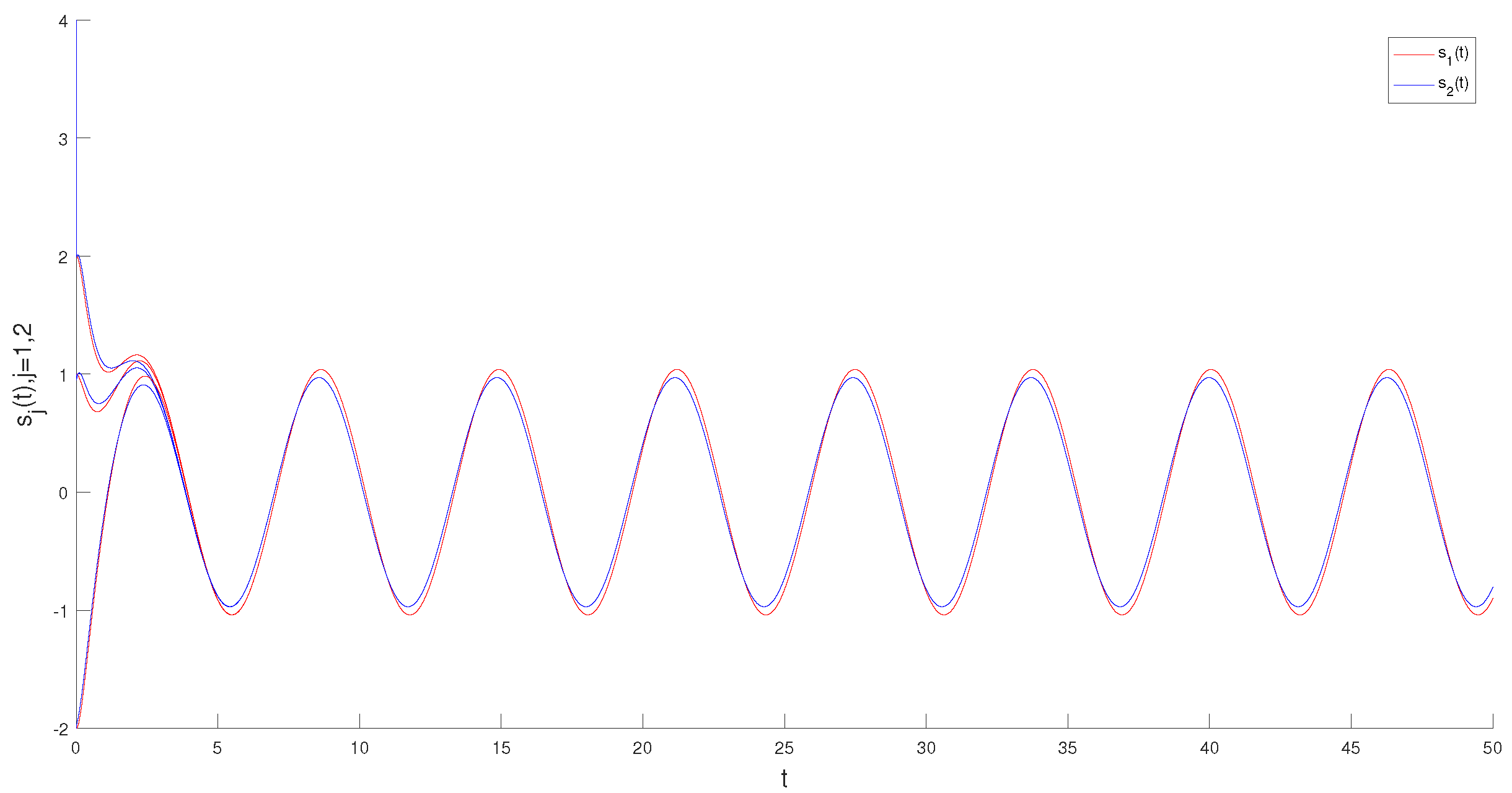
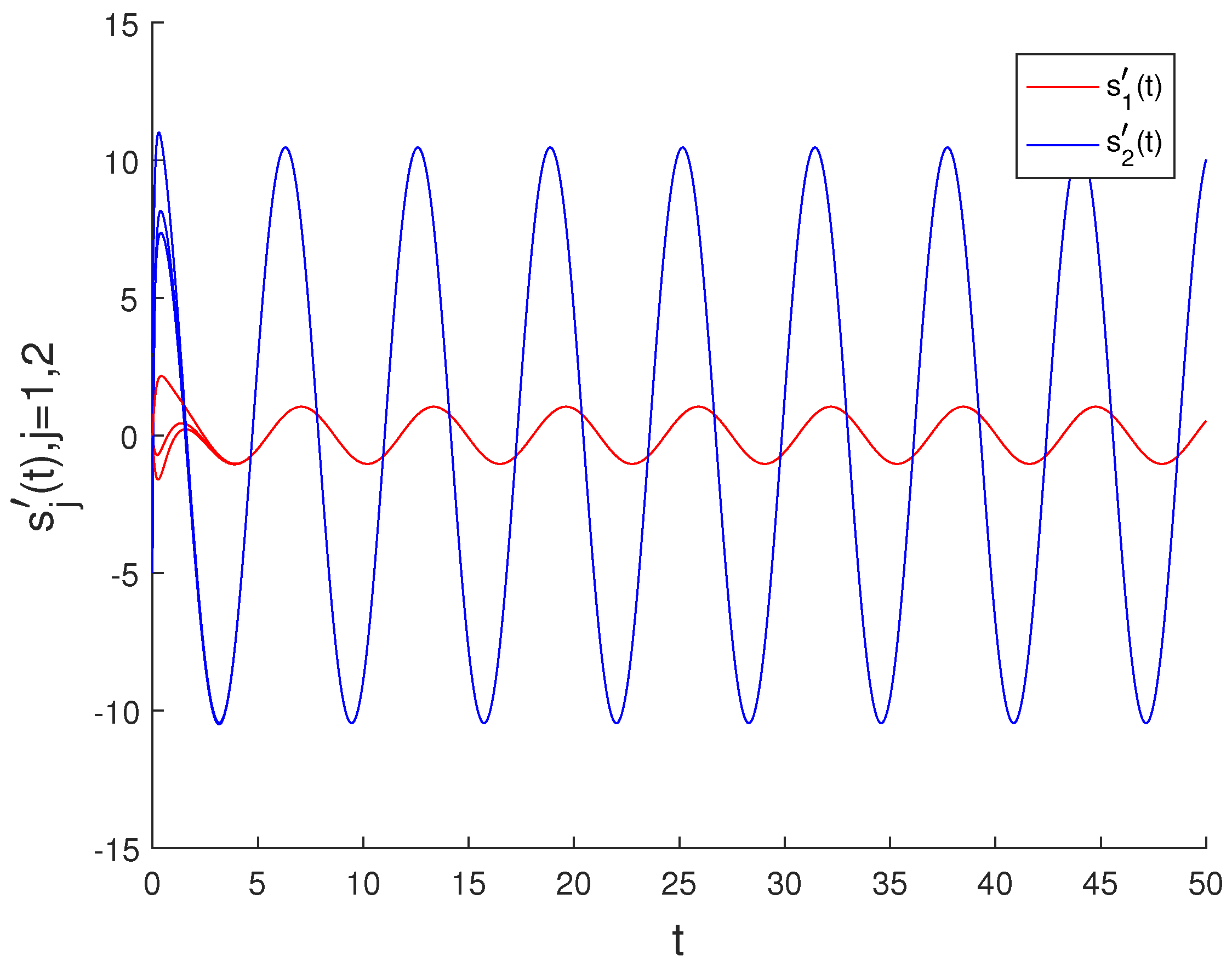
By utilizing Theorem 1, the NTINNs (40) possess a globally exponentially stable $2\pi$-periodic solution $x\left(t\right)$, and all solutions of (40) and their derivatives are exponentially convergent to $x\left(t\right)$ and $x^{\prime }\left(t\right)$, respectively. The simulation results of Figure 1 and Figure 2 show that the theoretical analysis is consistent with the numerical observation results.

Remark 3.

Since the global exponential stability of the T-periodic solutions on NTINNs involving multiple delays has never been studied, one can see that all the conclusions in references [42,43,44,45,46,47,48,49,50,51,52,53,54,55,56,57,58,59,60,61,62,63,64,65,66,67,68,69] cannot be directly employed to verify the global exponential stability of the $2\pi$-periodic solutions for NTINNs (40).

5. Conclusions

In this article, we researched the problem of the periodic solutions on NTINNs involving multiple delays. First, by exploring Lyapunov theory and inequality analysis, we establish the exponential attractivity of all solutions. Second, we obtained the existence of periodic solutions and their exponential stability. The effectiveness of the obtained results has been illustrated by an instructive numerical simulation. In addition, the method applied in this article offers a possible way to investigate the dynamic characteristics of other NTINNs, such as NTINNs involving D operators, fuzzy NTINNs, Cohen–Grossberg NTINNs and others.

References

- Babcock, K.; Westervelt, R. Stability and dynamics of simple electronic neural networks with added inertia. Physica D 1986, 23, 142–149. [Google Scholar] [CrossRef]
- Babcock, K.; Westervelt, R. Dynamics of simple electronic neural networks. Physica D 1987, 28, 305–316. [Google Scholar] [CrossRef]
- Shi, M.; Guo, J.; Fang, X.; Huang, C. Global exponential stability of delayed inertial competitive neural networks. Adv. Differ. Equ. 2020, 87. [Google Scholar] [CrossRef]
- Li, H.; Li, C.; Ouyang, D.; Nguang, S.K. Impulsive synchronization of unbounded delayed inertial neural networks with actuator saturation and sampled-data control and its application to image encryption. IEEE Trans. Neural Netw. Learn. Syst. 2021, 32, 1460–1473. [Google Scholar] [CrossRef] [PubMed]
- Zhang, Z.; Chen, M.; Li, A. Further study on finite-time synchronization for delayed inertial neural networks via inequality skills. Neurocomputing 2020, 375, 15–23. [Google Scholar] [CrossRef]
- Wang, L.; Huang, T.; Xiao, Q. Lagrange stability of delayed switched inertial neural networks. Neurocomputing 2020, 381, 52–60. [Google Scholar] [CrossRef]
- Kong, F.; Zhu, Q.; Sakthivel, R.; Mohammadzadeh, A. Fixed-time synchronization analysis for discontinuous fuzzy inertial neural networks with parameter uncertainties. Neurocomputing 2021, 422, 295–313. [Google Scholar] [CrossRef]
- Kong, F.; Zhu, Q.; Huang, T. New fixed-time stability lemmas and applications to the discontinuous fuzzy inertial neural networks. IEEE Trans. Fuzzy Syst. 2020. [Google Scholar] [CrossRef]
- Wang, J.; Wang, Z.; Chen, X.; Qiu, J. Synchronization criteria of delayed inertial neural networks with generally Markovian jumping. Neural Netw. 2021, 139, 64–76. [Google Scholar] [CrossRef]
- Liu, Y.; Wu, J.; Wang, X. Collective periodic motions in a multiparticle model involving processing delay. Math. Methods Appl. Sci. 2020, 44, 3280–3302. [Google Scholar] [CrossRef]
- Wei, X.; Zhang, Z.; Lin, C.; Chen, J. Synchronization and anti-synchronization for complex-valued inertial neural networks with time-varying delays. Appl. Math. Comput. 2021, 403, 126194. [Google Scholar] [CrossRef]
- Li, X.; Li, X.; Hu, C. Some new results on stability and synchronization for delayed inertial neural networks based on non-reduced order method. Neural Netw. 2017, 96, 91–100. [Google Scholar] [CrossRef] [PubMed]
- Huang, C.; Liu, B. New studies on dynamic analysis of inertial neural networks involving non-reduced order method. Neurocomputing 2019, 325, 283–287. [Google Scholar] [CrossRef]
- Zhang, J.; Huang, C. Dynamics analysis on a class of delayed neural networks involving inertial terms. Adv. Differ. Equ. 2020, 120. [Google Scholar] [CrossRef]
- Cao, Q.; Long, X. New convergence on inertial neural networks with time-varying delays and continuously distributed delays. AIMS Math. 2020, 5, 5955–5968. [Google Scholar] [CrossRef]
- Cai, Z.; Huang, J.; Yang, L.; Huang, L. Periodicity and stabilization control of the delayed filippov system with perturbation. D Contin. Dyn. Syst.-Ser. B 2020, 25, 1439–1467. [Google Scholar] [CrossRef] [Green Version]
- Cao, Q.; Guo, X. Anti-periodic dynamics on high-order inertial Hopfield neural networks involving time-varying delays. AIMS Math. 2020, 5, 5402–5421. [Google Scholar] [CrossRef]
- Yao, L.; Cao, Q. Anti-periodicity on high-order inertial Hopfield neural networks involving mixed delays. J. Inequal. Appl. 2020, 182. [Google Scholar] [CrossRef]
- Shi, J.; Zeng, Z. Global exponential stabilization and lag synchronization control of inertial neural networks with time delays. Neural Netw. 2020, 126, 11–20. [Google Scholar] [CrossRef]
- Yu, J.; Hu, C.; Jiang, H.; Wang, L. Exponential and adaptive synchronization of inertial complex-valued neural networks: A non-reduced order and non-separation approach. Neural Netw. 2020, 124, 20–59. [Google Scholar] [CrossRef]
- Wu, K.; Jian, J. Non-reduced order strategies for global dissipativity of memristive neutral-type inertial neural networks with mixed time-varying delays. Neurocomputing 2021, 436, 174–183. [Google Scholar] [CrossRef]
- Yu, F.; Qian, S.; Chen, X.; Huang, Y.; Liu, L.; Shi, C.; Cai, S.; Song, Y.; Wang, C. A new 4D four-wing memristive hyperchaotic system: Dynamical analysis, electronic circuit design, shape synchronization and secure communication. Int. J. Bifurc. Chaos 2020, 30, 2050147. [Google Scholar] [CrossRef]
- Gao, Z.; Wang, Y.; Xiong, J.; Pan, Y.; Huang, Y. Structural balance control of complex dynamical networks based on state observer for dynamic connection relationships. Complexity 2020, 2020, 5075487. [Google Scholar] [CrossRef]
- Li, W.; Huang, L.; Ji, J. Globally exponentially stable periodic solution in a general delayed predator-prey model under discontinuous prey control strategy. Discret. Contin. Dyn. Syst.-Ser. B 2020, 25, 2639–2664. [Google Scholar] [CrossRef] [Green Version]
- Zhu, Q.; Li, X. Exponential and almost sure exponential stability of stochastic fuzzy delayed Cohen-Grossberg neural networks. Fuzzy Sets Syst. 2012, 203, 74–94. [Google Scholar] [CrossRef]
- Zhang, X.; Hu, H. Convergence in a system of critical neutral functional differential equations. Appl. Math. Lett. 2020, 107, 106385. [Google Scholar] [CrossRef]
- Tan, T. Dynamics analysis of mackey-glass model with two variable delays. Math. Biosci. Eng. 2020, 17, 4513–4526. [Google Scholar] [CrossRef]
- Hale, J.K. Theory of Functional Differential Equations; Springer: New York, NY, USA, 1977. [Google Scholar]
- Zhang, X.; Han, Q. A new stability criterion for a partial element equivalent circuit model of neutral type. IEEE Trans. Circuits Syst. II Express Briefs 2009, 56, 798–802. [Google Scholar] [CrossRef]
- Jian, J.; Duan, L. Finite-time synchronization for fuzzy neutral-type inertial neural networks with time-varying coefficients and proportional delays. Fuzzy Sets Syst. 2020, 381, 51–67. [Google Scholar] [CrossRef]
- Lakshmanana, S.; Lima, C.P.; Prakashb, M.; Nahavandia, S.; Balasubramaniam, P. Neutral-type of delayed inertial neural networks and their stability analysis using the LMI Approach. Neurocomputing 2017, 230, 243–250. [Google Scholar] [CrossRef]
- Xu, M.; Du, B. Periodic solution for neutral-type inertial neural networks with time-varying delays. Adv. Differ. Equ. 2020, 607. [Google Scholar] [CrossRef]
- Guo, X.; Huang, C.; Cao, J. Nonnegative periodicity on high-order proportional delayed cellular neural networks involving D operator. AIMS Math. 2021, 6, 2228–2243. [Google Scholar] [CrossRef]
- Huang, C.; Yang, H.; Cao, J. Weighted pseudo almost periodicity of multi-proportional delayed shunting inhibitory cellular neural networks with D operator. Discret. Contin. Dyn. Syst. Ser. S 2021, 14, 1259–1272. [Google Scholar] [CrossRef]
- Chen, D.; Zhang, W.; Cao, J.; Huang, C. Fixed time synchronization of delayed quaternion-valued memristor-based neural networks. Adv. Differ. Equ. 2020, 2020, 92. [Google Scholar] [CrossRef]
- Cai, Z.; Huang, L.; Wang, Z. Mono/multi-periodicity generated by impulses control in time-delayed memristor-based neural networks. Nonlinear Anal.-Hybrid Syst. 2020, 36, 100861. [Google Scholar] [CrossRef]
- Huang, C.; Long, X.; Cao, J. Stability of anti-periodic recurrent neural networks with multiproportional delays. Math. Methods Appl. Sci. 2020, 43, 6093–6102. [Google Scholar] [CrossRef]
- Xu, C.; Liao, M.; Li, P.; Guo, Y.; Xiao, Q.; Yuan, S. Influence of multiple time delays on bifurcation of fractional-order neural networks. Appl. Math. Comput. 2019, 361, 565–582. [Google Scholar] [CrossRef]
- Faydasicok, O. New criteria for global stability of neutral-type Cohen-Grossberg neural networks with multiple delays. Neural Netw. 2020, 125, 330–337. [Google Scholar] [CrossRef]
- Iswarya, M.; Raja, R.; Rajchakit, G.; Cao, J.; Alzabut, J.; Huang, C. Existence, uniqueness and exponential stability of periodic solution for discrete-time delayed BAM neural networks based on coincidence degree theory and graph theoretic method. Mathematics 2019, 7, 1055. [Google Scholar] [CrossRef] [Green Version]
- Yang, H. Weighted pseudo almost periodicity on neutral type CNNs involving multi-proportional delays and D operator. AIMS Math. 2021, 6, 1865–1879. [Google Scholar] [CrossRef]
- Huang, C.; Long, X.; Huang, L.; Fu, S. Stability of almost periodic Nicholson’s blowflies model involving patch structure and mortality terms. Canad. Math. Bull. 2020, 63, 405–422. [Google Scholar] [CrossRef]
- Huang, C.; Tan, Y. Global behavior of a reaction-diffusion model with time delay and Dirichlet condition. J. Differ. Equ. 2021, 271, 186–215. [Google Scholar] [CrossRef]
- Huang, C.; Zhang, H.; Cao, J.; Hu, H. Stability and Hopf bifurcation of a delayed prey-predator model with disease in the predator. Internat. J. Bifur. Chaos Appl. Sci. Engrg. 2019, 29, 1950091. [Google Scholar] [CrossRef]
- Huang, C.; Zhang, H.; Huang, L. Almost periodicity analysis for a delayed Nicholson’s blowflies model with nonlinear density-dependent mortality term. Commun. Pure Appl. Anal. 2019, 18, 3337–3349. [Google Scholar] [CrossRef] [Green Version]
- Long, X. Novel stability criteria on a patch structure Nicholson’s blowflies model with multiple pairs of time-varying delays. AIMS Math. 2020, 5, 7387–7401. [Google Scholar] [CrossRef]
- Huang, C.; Zhao, X.; Cao, J.; Alsaadi, F.E. Global dynamics of neoclassical growth model with multiple pairs of variable delays. Nonlinearity 2020, 33, 6819–6834. [Google Scholar] [CrossRef]
- Huang, C.; Wang, J.; Huang, L. Asymptotically almost periodicity of delayed Nicholson-type system involving patch structure. Electron. J. Differ. Equ. 2020, 102. [Google Scholar] [CrossRef]
- Huang, C.; Zhang, J.; Cao, J. Delay-dependent attractivity on a tick population dynamics model incorporating two distinctive time-varying delays. Proc. R. Soc. A-Math. Phys. Eng. Sci. 2021, 447, 20210302. [Google Scholar] [CrossRef]
- Long, X.; Gong, S. New results on stability of Nicholson’s blowflies equation with multiple pairs of time-varying delays. Appl. Math. Lett. 2020, 2020, 106027. [Google Scholar] [CrossRef]
- Qian, C.; Hu, Y. Novel stability criteria on nonlinear density-dependent mortality Nicholson’s blowflies systems in asymptotically almost periodic environments. J. Inequal. Appl. 2020, 13. [Google Scholar] [CrossRef]
- Xu, C.; Li, P.; Xiao, Q.; Yuan, S. New results on competition and cooperation model of two enterprises with multiple delays and feedback controls. Bound. Value Probl. 2019, 36. [Google Scholar] [CrossRef]
- Hu, H.; Yuan, X.; Huang, L.; Huang, C. Global dynamics of an sirs model with demographics and transfer from infectious to susceptible on heterogeneous networks. Math. Biosci. Eng. 2019, 16, 5729–5749. [Google Scholar] [CrossRef] [PubMed]
- Duan, L.; Huang, L.; Guo, Z.; Fang, X. Periodic attractor for reaction-diffusion high-order Hopfield neural networks with time-varying delays. Comput. Math. Appl. 2017, 73, 233–245. [Google Scholar] [CrossRef]
- Cai, Z.; Huang, J.; Huang, L. Generalized Lyapunov-Razumikhin method for retarded differential inclusions: Applications to discontinuous neural networks. Discret. Contin. Dyn. Syst.-Ser. B 2017, 22, 3591–3614. [Google Scholar] [CrossRef] [Green Version]
- Zhang, H.; Qian, C. Convergence analysis on inertial proportional delayed neural networks. Adv. Differ. Equ. 2020, 277. [Google Scholar] [CrossRef]
- Pratap, A.; Raja, R.; Cao, J.; Huang, C.; Niezabitowski, M.; Bagdasar, O. Stability of discrete-time fractional-order time-delayed neural networks in complex field. Math. Meth. Appl. Sci. 2020, 44, 419–440. [Google Scholar] [CrossRef]
- Wei, R.; Cao, J.; Huang, C. Lagrange exponential stability of quaternion-valued memristive neural networks with time delays. Math. Meth. Appl. Sci. 2020, 43, 7269–7291. [Google Scholar] [CrossRef]
- Pratap, A.; Raja, R.; Cao, J.; Alzabut, J.; Huang, C. Finite-time synchronization criterion of graph theory perspective fractional-order coupled discontinuous neural networks. Adv. Differ. Equ. 2020, 97. [Google Scholar] [CrossRef] [Green Version]
- Wang, P.; Hu, H.; Jun, Z.; Tan, Y.; Liu, L. Delay-Dependent Dynamics of Switched Cohen-Grossberg Neural Networks with Mixed Delays. Abstr. Appl. Anal. 2013, 2013, 826426. [Google Scholar] [CrossRef] [Green Version]
- Pratap, A.; Raja, R.; Alzabut, J.; Cao, J.; Rajchakit, G.; Huang, C. Mittag-leffler stability and adaptive impulsive synchronization of fractional order neural networks in quaternion field. Math. Meth. Appl. Sci. 2020, 43, 6223–6253. [Google Scholar] [CrossRef]
- Rajchakit, G.; Pratap, A.; Raja, R.; Cao, J.; Alzabut, J.; Huang, C. Hybrid Control Scheme for Projective Lag Synchronization of Riemann–Liouville Sense Fractional Order Memristive BAM NeuralNetworks with Mixed Delays. Mathematics 2019, 7, 759. [Google Scholar] [CrossRef] [Green Version]
- Iswarya, M.; Raja, R.; Rajchakit, G.; Cao, J.; Alzabut, J.; Huang, C. A perspective on graph theory-based stability analysis of impulsive stochastic recurrent neural networks with time-varying delays. Adv. Differ. Equ. 2019, 502. [Google Scholar] [CrossRef] [Green Version]
- Kuang, H.; Liu, J.; Chen, X.; Mao, J.; He, L. Asymptotic Behavior of Switched Stochastic Delayed Cellular Neural Networks via Average Dwell Time Method. Abstr. Appl. Anal. 2013, 2013, 270791. [Google Scholar] [CrossRef] [Green Version]
- Zhu, Q.; Huang, C.; Yang, X. Exponential stability for stochastic jumping BAM neural networks with time-varying and distributed delays. Nonlinear Anal.-Hybrid Syst. 2011, 5, 52–77. [Google Scholar] [CrossRef]
- Li, L.; Wang, W.; Huang, L.; Wu, J. Some weak flocking models and its application to target tracking. J. Math Anal. Appl. 2019, 480, 123404. [Google Scholar] [CrossRef]
- Manickam, I.; Ramachandran, R.; Rajchakit, G.; Cao, J.; Huang, C. Novel lagrange sense exponential stability criteria for time-delayed stochastic cohen-grossberg neural networks with markovian jump parameters: A graph-theoretic approach. Nonlinear Anal.-Model Control 2020, 25, 726–744. [Google Scholar] [CrossRef]
- Huang, C.; Liu, B.; Qian, C.; Cao, J. Stability on positive pseudo almost periodic solutions of HPDCNNs incorporating D operator. Math. Comput. Simul. 2021, 190, 1150–1163. [Google Scholar] [CrossRef]
- Xu, C.; Li, P.; Liao, M.; Liu, Z.; Xiao, Q. Antiperiodic solutions to delayed inertial quaternion-valued neural networks. Math. Methods Appl. Sci. 2020, 43, 7326–7344. [Google Scholar] [CrossRef]
Figure 1.
Numerical solutions on NTINNs (40) incorporating different initial values.
Figure 2.
The derivative on NTINNs (40) incorporating different initial values.
Publisher’s Note: MDPI stays neutral with regard to jurisdictional claims in published maps and institutional affiliations. |
© 2021 by the authors. Licensee MDPI, Basel, Switzerland. This article is an open access article distributed under the terms and conditions of the Creative Commons Attribution (CC BY) license (https://creativecommons.org/licenses/by/4.0/).
Share and Cite
MDPI and ACS Style
Zhang, J.; Chang, A.; Yang, G. Periodicity on Neutral-Type Inertial Neural Networks Incorporating Multiple Delays. Symmetry 2021, 13, 2231. https://0-doi-org.brum.beds.ac.uk/10.3390/sym13112231
AMA Style
Zhang J, Chang A, Yang G. Periodicity on Neutral-Type Inertial Neural Networks Incorporating Multiple Delays. Symmetry. 2021; 13(11):2231. https://0-doi-org.brum.beds.ac.uk/10.3390/sym13112231
Chicago/Turabian StyleZhang, Jian, Ancheng Chang, and Gang Yang. 2021. "Periodicity on Neutral-Type Inertial Neural Networks Incorporating Multiple Delays" Symmetry 13, no. 11: 2231. https://0-doi-org.brum.beds.ac.uk/10.3390/sym13112231
Note that from the first issue of 2016, this journal uses article numbers instead of page numbers. See further details here.