Research on Optimization of Urban Public Transport Network Based on Complex Network Theory

Abstract

The urban public transportation system is an important part of urban transportation, and the rationality of public transportation routes layout plays a vital role in the transportation of the city. Improving the efficiency of public transportation can have a positive impact on the operation of the public transportation system. This paper uses complex network theory and the symmetry of the up and down bus routes and stations to establish an urban public transit network model and calculates the probability of passengers choosing different routes in the public transit network according to passenger travel impedance. Based on passenger travel impedance, travel path probability and passenger travel demand, the links are weighed, and the network efficiency calculation method is improved. Finally, the public transit network optimization model was established with network efficiency as the objective function and solved by the ant colony algorithm. In order to verify the effectiveness of the model and the solution method, this paper selects areas in Nanguan District of Changchun City for example analysis. The result shows that the efficiency of the optimized network is 8.5% higher than that of the original network, which proves the feasibility of the optimized model and solution method.

1. Introduction

With the rapid development of China’s economy, the scale of cities and the ownership of cars have increased [1]. Currently, the development of urban transportation in China lags in the development of urban economy. Therefore, a series of traffic problems has appeared in the process of urbanization, such as serious traffic congestion during peak travel times, frequent traffic accidents, significant difficulty in parking, etc. In the urban transportation system, urban public transportation has become one of the main travel modes of residents due to the advantages of large passenger capacity, low travel cost and wide coverage. At the same time, the development of the public transportation system has effectively alleviated traffic congestion and other traffic problems; thus, the development of urban public transportation and the encouragement of green public transportation have become the main development goals of urban transportation [2].

Urban rail transit and conventional transit are important components of the urban public transportation system, and the rationality of the layout plays a vital role in the transportation of the city. Due to the late beginning of the construction of urban rail transit in China and the relatively short development time, the city failed to form a reasonable public transportation system. There are many problems in the network layout, and one of the most important problem is that public transportation routes cannot complement each other’s advantages, and there is vicious competition, which renders the overall public transportation system inefficient.

With the rapid development of computer technology, complex network theory can be applied to all fields of life [3,4]. When road conditions permit, the driving routes and stations of the up and down bus routes are symmetrical; thus, urban public transportation can be abstracted as an upline transit network and a downline transit network. According to complex network theory, the overall level of the public transportation network can be described scientifically and comprehensively, and it can also objectively reflect the connection of various routes and stations in the bus route network [5]. As early as 2000, some scholars have carried out research on the application of complex networks to transportation networks. In the literature [6], the study modeled the world aviation network and analyzed network topology. Finally, this study found that network topology has a scale-free characteristic. A typical research study on the application of complex network theory to public transportation systems is Ref. [7]; the study used the Space L method and Space P method separately to model the public transit network of 22 cities in Poland and systematically analyzed the statistical characteristics of network topology.

Due to the fact that the public transportation system is complex, the powerless network cannot show a real public transportation system. Many scholars have carried out research on the empowerment of the public transit network. Yang J et al. [8] weighted the public transit network with cross-sectional passenger flow, and they found that the weighted invulnerability measurement index can better describe the robustness of the network. Lu Q et al. [9] used passenger travel time and passenger flow as weights for the rail transit network. The research results show that the failure of stations with high time weighting and passenger flow centrality in the weighted rail transit network can cause a greater loss of average travel time for users. Zhou Y [10] used the PTEW weighting method to assign weights to the public transit network. The study introduced the BPR function in order to reflect public travel time cost and used PTEW weighting to calculate traffic impedance of each section. Finally, the author used the impedance and the transit time of the station as weights. Cats O et al. [11] took passenger flow in the route as the weight of the link. So far, most of the existing research studies considered single factors such as cross-section passenger flow, travel time or impedance in order to provide weight to the network but only considering that single factors cannot reflect the true network operation status. These factors need to be considered comprehensively to weight the network.

In terms of public transit network optimization, Ding J et al. [12] established an optimization model of the public transit network for the dual goals of bus station optimization and bus routes optimization based on the direct accessibility of the stations and optimized the public transit network by using the K shortest path algorithm. Lu H et al. [13] considered the influence of travel behavior in route layout and built a double-layer optimization model based on the spatial topological structure of rail transit routes and bus routes, while optimizing bus routes and departure intervals. Wang F [14] constructed a bus–subway weighted composite network based on card swiping data of the bus and subway and optimized the bus route network. Network efficiency was improved based on the traffic efficiency of the link. Finally, the author took the improved network efficiency as the optimization goal and used the addition and deletion of stations as the optimization method. Hao Y [15] put forward the idea of hierarchical optimization of multi-mode public transit network. The optimization goal of the main route network was to reduce the negative effect of travel, and the optimization goal of the branch route network was to increase the coverage of the route network. The ant colony algorithm was used to achieve route network optimization. Some classic studies are provided in

Table 1. Literature review.

Reference	Empowerment Factor	Modeling Method	Optimization Goals
Zhou X (2016) [16]	Number of routes	Space L, Space P, Space R	Unoptimized
Peng J (2017) [17]	Transit passenger capacity, distance between stations	Space L, Space P, Space R	Unoptimized
Lai Q (2021) [18]	Unweighted	Space L	Network robustness
Cao Z (2020) [19]	Travel time	Space P	Total travel time
Chen X (2020) [20]	Betweenness centrality, intimacy centrality, degree centrality	Space M	Network efficiency

. The existing research studies lack consideration of the overall network in the selection of the optimization goal of the public transit network, such as [12,13,15], or achieves the optimization of the overall efficiency of the network but ignores the influence of the direction of the bus routes, such as [14]. The overall efficiency of the public transit network should be optimized while considering changes in bus routes.

This paper proposes a new transit network optimization model. In this model, the passenger travel path selection probability is determined by passenger travel impedance; the network weight is calculated by passenger travel impedance, travel path selection probability and passenger demand; and the objective function is the improved network efficiency. Finally, the model is solved by using the ant colony algorithm in order to improve urban public transport operation efficiency. It alleviates the problem that the layout of urban bus lines is unreasonable and the operation efficiency of public transport system is low.

2. Materials and Methods

The mainstream method of modeling conventional bus network and rail transit network based on complex network theory can be divided into two types [16]: one is to build a network representation model based on the route (Space R modeling method) and the other class is based on the station to build a network representation model (Space L modeling method and Space P modeling method). The Space P modeling method and Space R modeling method have a clearer performance on the transfer between routes in the bus network. They are mainly used to analyze the transfer between routes and cannot fully reflect the true topological relationship of the network. Therefore, this paper uses the Space L model method to establish the urban public transit network model. Considering the symmetry of the driving routes and stations of the up and down bus routes, the same name stations with less than 50 m on both sides of the road were merged in the modeling process. The up and down transit routes are abstracted as one line, and the constructed network is a directed network.

This paper uses a generalized travel cost function to quantitatively express the interference effects of vehicles, roads and the environment on public transportation travel. Based on the urban public transit network model, a generalized cost is used to comprehensively consider the impedance of bus travel from the origin and destination of various main factors; the generalized travel cost can be expressed by the following.

Generalized travel cost = Waiting time + In vehicle time + Transfer time

(1)

The waiting time of passengers at the station is an indeterminate value. This time is mainly related to the number of passenger transfers and the probability distribution of the headway time. When the route chosen by the passenger does not require transfers and if the vehicle arriving at the station obeys a uniform distribution, the maximum waiting time is the headway of the vehicle and the minimum is 0. Let $x_a$ (2) and $h_a$ (2), respectively, denote waiting time and headway; the probability density function of waiting time can be expressed by the following.

$$f_{x_a}\left(x_a\right)=\frac{1}{h_a}\left(0\le x_a\le h_a\right)$$

(2)

If passengers take route a and then transfer to route b, the headway of route a and route b are, respectively, $h_a$ (3) and $h_b$ (3), and the total waiting time is set to z (3). If the arrival times of route a and route b are uniform distribution, the probability density function of the total waiting time can be expressed by the following.

$$f_z(z)=\{\begin{array}{cc}\frac{z}{h_a\cdot h_b}\hfill & 0\le z\le h_a\hfill \\ \frac{1}{h_b}\hfill & h_a\le z\le h_b\hfill \\ \frac{h_a+h_b-z}{h_a\cdot h_b}\hfill & h_b\le z\le (h_a+h_b)\hfill \end{array}$$

(3)

The derivation process is shown in Appendix A.

The vehicle time of passengers can be divided into vehicle stopping time at a station and vehicle travel time between stations. In the public transportation system, vehicle stopping time can be divided into two types, fixed stopping time and stopping time, that varies with the number of up and down passengers. The former is mainly used in rail transit, especially subway and light rail systems, while the latter is suitable for most rapid transit and conventional buses.

Let $v_s$ (4) and (5), $d_{ij}$ (4) and (5), and T, respectively, denote vehicle speed, the distance between stations i and j, and the stopping time of rail transit vehicles. For rail transit and conventional buses with dedicated tracks/lanes, the travel time between adjacent stations can be expressed by the following [21].

$$t_i^g=\frac{d_{ij}}{v_s}+T$$

(4)

For conventional transit, let $p{t}_l^i$ (5) and α_ij (5), respectively, denote the stopping time of conventional transit vehicles and road congestion factor. Due to the fact that the speed of the vehicle is greatly affected by the traffic environment, the speed of each road section may be different; thus, vehicle travel time between adjacent nodes can be expressed by the following.

$$t_i^c=\frac{d_{ij}}{{\alpha }_{ij}\cdot v_s}+p{t}_l^i$$

(5)

When a bus has no priority at a road intersection, it is affected by signal control and can cause road intersection delays. For rail transit, its routes are independent, and there is no delay at road intersections; for other conventional bus routes, this paper assumes that road intersection delay t_y (6) is the same as other vehicles. The sum of vehicle travel time between the stations, vehicle stopping time at station and the delay of the intersection is the boundary impedance between adjacent nodes, which is described as follows:

$$Z_o=\beta \cdot t_i^g+\lambda \cdot \left(t_i^c+m\cdot t_y\right)$$

(6)

where β (6) and λ (6) are category parameters. If the link belongs to rail transit, then β is 1 and λ is 0. If the link belongs to conventional transit, then λ is 1 and β is 0.

Transfers between public transports are mainly divided into transfers at the same station and transfers between different stations. The time spent on transferring at the same station is mainly the waiting time. In addition to the waiting time, the transfer between stations also includes the walking time between stations. In the process of transferring at the same station, passengers only need to continue to wait for the transfer route vehicle at the original station after getting off the bus without walking; thus, the impedance of the same station transfer is the waiting time. Compared with transferring at the same station, transferring at different stations includes the walking time between stations and the transfer penalty coefficient. Transfer impedance can be expressed as the product of the transfer penalty coefficient μ (7) and walking time, and the walking time is the ratio of the distance between stations d (7) and the walking speed v (7).

$$Z_h=\mu \cdot \frac{d}{v}$$

(7)

Finally, the travel impedance from node o to node d can be expressed by the following.

$$Z_{od}={\displaystyle {\sum }_{i_o\le i<i_d}\left[\beta \cdot t_i^g+\lambda \cdot \left(t_i^c+m\cdot t_y\right)+\mu \cdot \frac{d}{v}\right]}$$

(8)

There are three types of links in the constructed public transit network: the links between notes in the conventional bus network, the links between notes in the rail transit network and the artificially added transfer links. This paper defines the weights of the public transit network links as follows.

$$W_{ij}^g=t_i^g\cdot \frac{{\displaystyle {\sum }_{a=1}^n{C}_{e,a}^g}}{{\displaystyle {\sum }_{a=1}^n{C}_{ij,a}^g}}$$

(9)

The calculation method for the weight of rail transit link can be expressed as formula (9), where n is the number of rail transit routes passing through nodes i and j, $C_{e,a}^g$ is the passenger capacity of rail transit route a and $C_{ij,a}^g$ is the passenger capacity of rail transit route a between nodes i and j.

$$W_{ij}^c=t_{i,l}^c\cdot \frac{{\displaystyle {\sum }_{a=1}^n{C}_{e,a}^c}}{{\displaystyle {\sum }_{a=1}^n{C}_{ij,a}^c}}$$

(10)

The calculation method for the weight of conventional bus link can be expressed as formula (10), where n is the number of conventional bus routes passing through nodes i and j, $C_{e,a}^c$ is the passenger capacity of conventional bus route a, and $C_{ij,a}^c$ is the passenger capacity of conventional bus route a between nodes i and j. The transfer link can be expressed by the following.

$$W_{ij}^h=Z_h^y$$

(11)

Latora et al. [22] first proposed the concept of network efficiency. Network efficiency is used to evaluate the overall operation of the network. The efficiency of any two nodes is defined as the reciprocal of the shortest path distance between two nodes. Network efficiency is the average of the efficiency between any two nodes. In the traditional network efficiency calculation process, the selection of the shortest path between nodes only considers the connection relationship between nodes and does not consider the weight of the network. The shortest path distance is the number of nodes passed by the shortest path, which cannot truly reflect the current status of the transportation network. Some scholars [14,23] improved the calculation method of network efficiency by using network weights but did not consider the uncertainty of passengers choosing travel paths; thus, this paper proposes a new calculation method.

The method of minimum comprehensive impedance is used to find the shortest path between nodes. In a real public transportation network, when passengers choose a path, there will be similar paths. With the application of intelligent public transportation systems and the popularization of various travel service software, passengers can easily obtain vehicle arrival time and waiting time; however, only considering the minimum total impedance between nodes may not be the optimal choice in some cases [24]. As shown in Figure 1, there are two paths from node A to node B. Path 1 is to take conventional bus route a, which is a total of 20 min; path 2 is to take rail transit route b and then transfer to rail transit route c, and the travel times of route b and route c are both 8 min. Only travel time is calculated, and path 2 is better than path 1; if the transfer time between route b and route c exceeds 4 min, path 1 is better than path 2. Thus, the process of finding the shortest path between nodes in this paper is as follows.

• Determine the shortest path according to the integrated impedance between nodes i and j;
• Determine the maximum travel time of the shortest path;
• Search for other paths to minimize comprehensive impedance. If the integrated impedance of a path is less than the maximum travel time of the shortest path, then the path is placed into the set of candidate paths;
• Traverse the set of candidate paths and determine the constraints for selecting the candidate paths;
• Calculate the probability of alternative paths meeting the constraints, sort the alternative paths according to the comprehensive impedance and output the shortest path set and probability of choice.

Assuming that there are two paths to choose, the probability density function of the total waiting time of path 1 is $f_{z_1}(z_1)$ (13), and the probability density function of the total waiting time of path 2 is $f_{z_2}(z_2)$ (13), and Z is defined as follows.

$$Z=\{\begin{array}{cc}1,\hfill & { z}_1\le z_2\hfill \\ 0,\hfill & { z}_1>z_2\hfill \end{array}$$

(12)

Due to the fact that z₁ and z₂ are independent of each other, the probability density of (z₁, z₂) can be expressed by the following.

$$f(z_1,z_2)=f_{Z_1}(z_1)\cdot f_{Z_2}(z_2)$$

(13)

The probability of choosing path 1 is as follows.

$$P\left\{Z=1\right\}={\displaystyle \underset{z_1\le z_2}{\iint }f(x,y)\mathrm{d}x\mathrm{d}y}$$

(14)

The probability of choosing path 2 is 1−P{Z = 1}. When there are more than two paths that can be selected, the calculation of the selection probability of each path becomes complicated. The simulation method can be selected to simulate the calculation of path selection probability.

Assuming that there are n (15) alternative paths between nodes i and j and the probabilities of choosing each path are P₁, P₂, …, P_n (15), the calculation formula for the efficiency between nodes i and j can be expressed by the following.

$$L_{ij}={\displaystyle {\sum }_{i=1}^n{P}_i}\cdot \left({\displaystyle {\sum }_{j=1}^{m_i}{W}_j}\right)$$

(15)

The calculation method to improve network efficiency can be expressed by the following.

$$E=\frac{1}{\frac{1}{2}n(n-1)}{\displaystyle {\sum }_{i>j}\frac{1}{L_{ij}}}=\frac{1}{\frac{1}{2}n(n-1)}{\displaystyle {\sum }_{i>j}\frac{1}{{\displaystyle {\sum }_{i=1}^n{P}_i}\cdot \left({\displaystyle {\sum }_{j=1}^{m_i}{W}_j}\right)}}$$

(16)

The optimization of the urban public transit network aims to improve the operation efficiency of the public transit network. The optimization goals of the urban public transportation network can be summarized as follows: to meet the travel needs of passengers in different regions; to reduce the time cost of taking public transportation; and to improve the utilization rate of public transportation resources and improve the operating efficiency of the network. There should be certain constraints in the optimization process of the public transportation network. The optimization method mainly optimizes conventional transit routes, and rail transit will not be adjusted. Constraint conditions are set in route length, route non-linear coefficient, station spacing, number of optimized routes and road network. The optimization goal is to improve network efficiency, and the public transit network optimization model is established as follows.

$$\begin{array}{c}\max E(G)=\frac{1}{\frac{1}{2}n(n-1)}{\displaystyle {\sum }_{i>j}\frac{1}{{\displaystyle {\sum }_{i=1}^n{P}_i}\cdot \left({\displaystyle {\sum }_{j=1}^{m_i}{W}_j}\right)}}\\ 3 \mathrm{km}\le L_g\le 20 \mathrm{km}\\ 3 \mathrm{km}\le L_z\le 10 \mathrm{km}\\ N_l=\frac{d}{L}\le 1.4\\ 300 \mathrm{m}\le l_{ij}\le 800 \mathrm{m}\\ N{L}_{line}\subset N{L}_{app}\\ N{L}_{line}\subseteq R{G}_{line}\end{array}$$

(17)

In Formula (17), $L_g$ is the length of the main bus route; $L_z$ is the length of the branch bus route; $N_l$ is the route non-linear coefficient; $l_{ij}$ is the distance between stations i and j; $N{L}_{line}$ is the optimized bus routes set; $N{L}_{app}$ is the set of roads that can be used by conventional transit; and $R{G}_{line}$ is the collection of bus routes that needs to be optimized.

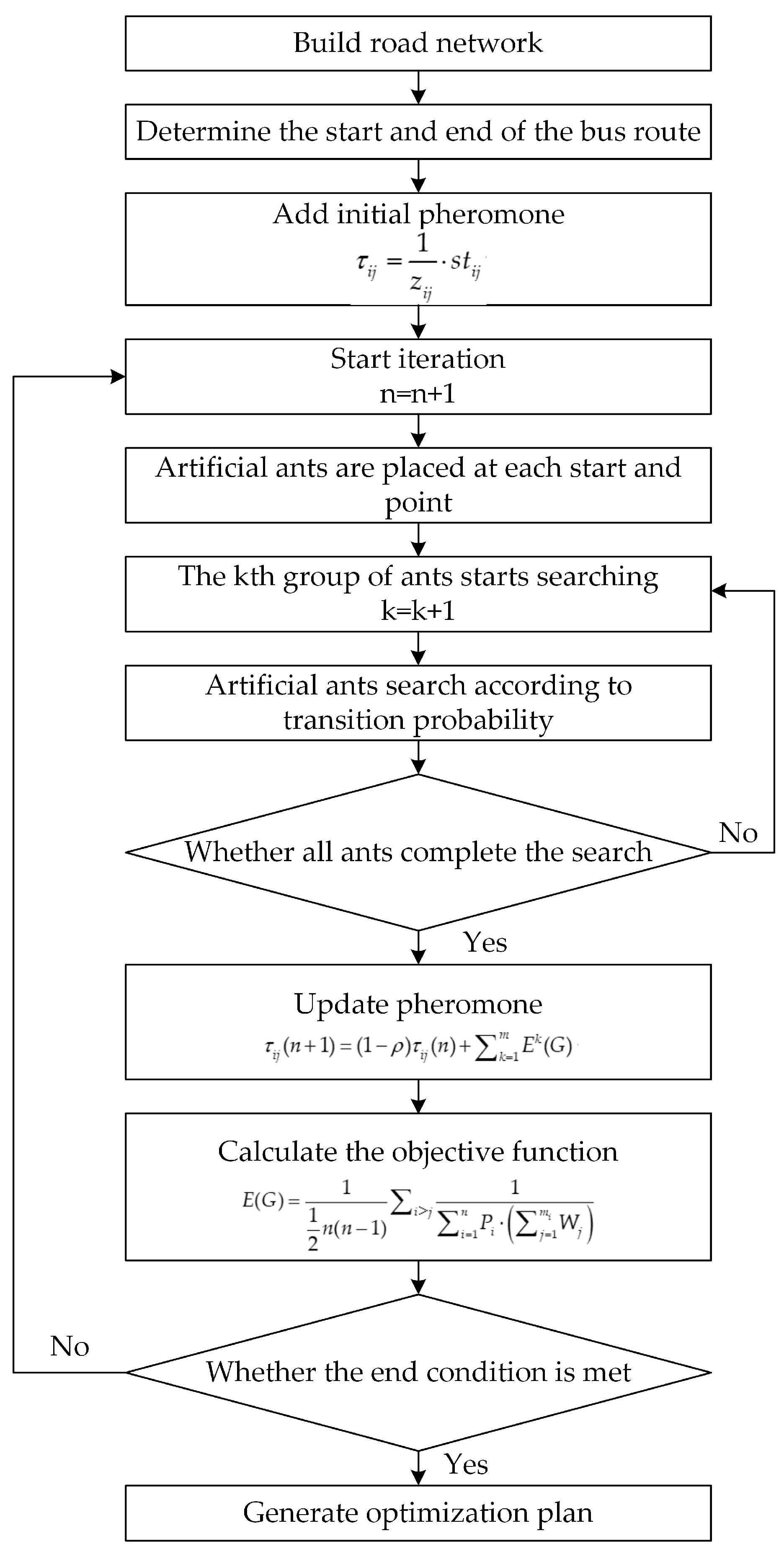
The optimization model is solved by the ant colony algorithm, and the initial pheromone is expressed by the following.

$${\tau }_{ij}=\frac{1}{z_{ij}}\cdot s{t}_{ij}$$

(18)

In formula (18), $z_{ij}$ is the travel impedance from node i to node j; and $s{t}_{ij}$ is the demand of bus travel on the link. The formula for pheromone updating is as follows.

$$\Delta {\tau }_{ij}={\displaystyle {\sum }_{k=1}^m{E}^k(G)}$$

(19)

In formula (19), $E^k(G)$ is the network efficiency of the network chosen by the kth group of ants. In order to avoid falling into the local optimum, pheromone has a lower limit ${\tau }_{\min }$. According to the basic principles of the ant colony algorithm, the solution steps for the optimization model of the public transport network are shown in Figure 2. The calculation method of pheromone update can be expressed by the following.

$${\tau }_{ij}(t+1)=(1-\rho ){\tau }_{ij}(t)+\Delta {\tau }_{ij}$$

(20)

$$\Delta {\tau }_{ij}={\displaystyle {\sum }_{k=1}^m{\tau }_{ij}^k(t+1)}$$

(21)

In Formula (20) and (21), t is the number of iterations, and $\rho$ is volatilization coefficient.

3. Results

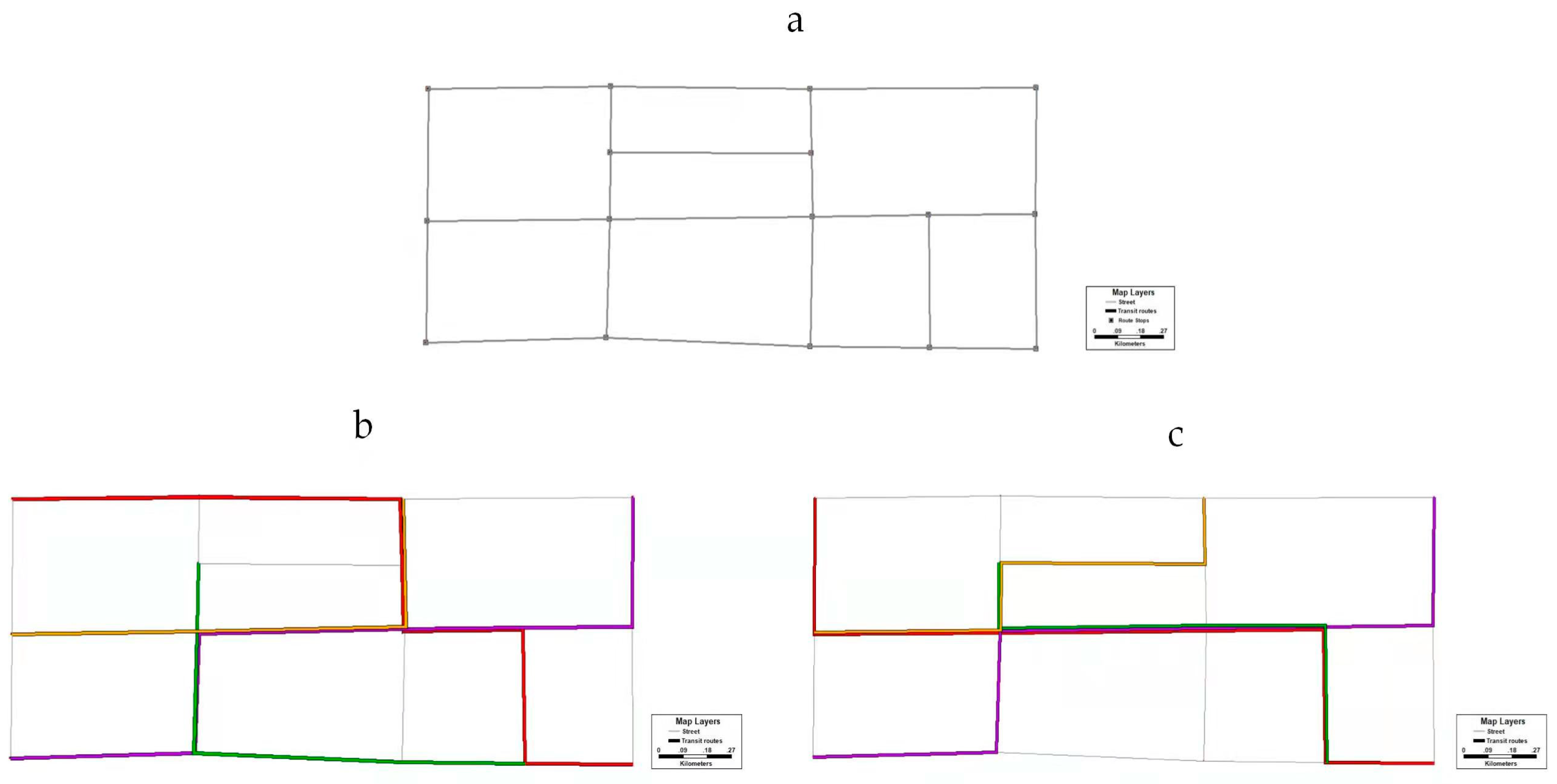
In this paper, a simple theoretical network is established in which passenger transport demand is a random number. The bus routes of the theoretical network are planned by the optimization method, which takes original network efficiency and improved network efficiency as the objective function, respectively. Figure 3b is the result of the original optimization method, Figure 3c is the result of the improved optimization method, and the parameters are set in

Table 2. Parameter value of ant colony algorithm.

Parameter	Number of Stations	Number of Ants	Volatilization Coefficient	Number of Iterations
Value	16	100	0.9	100

. The network efficiency of the original optimization method is 0.23312 and that of the improved optimization method is 0.25513. The optimization result of the improved method is higher than that of the original method.

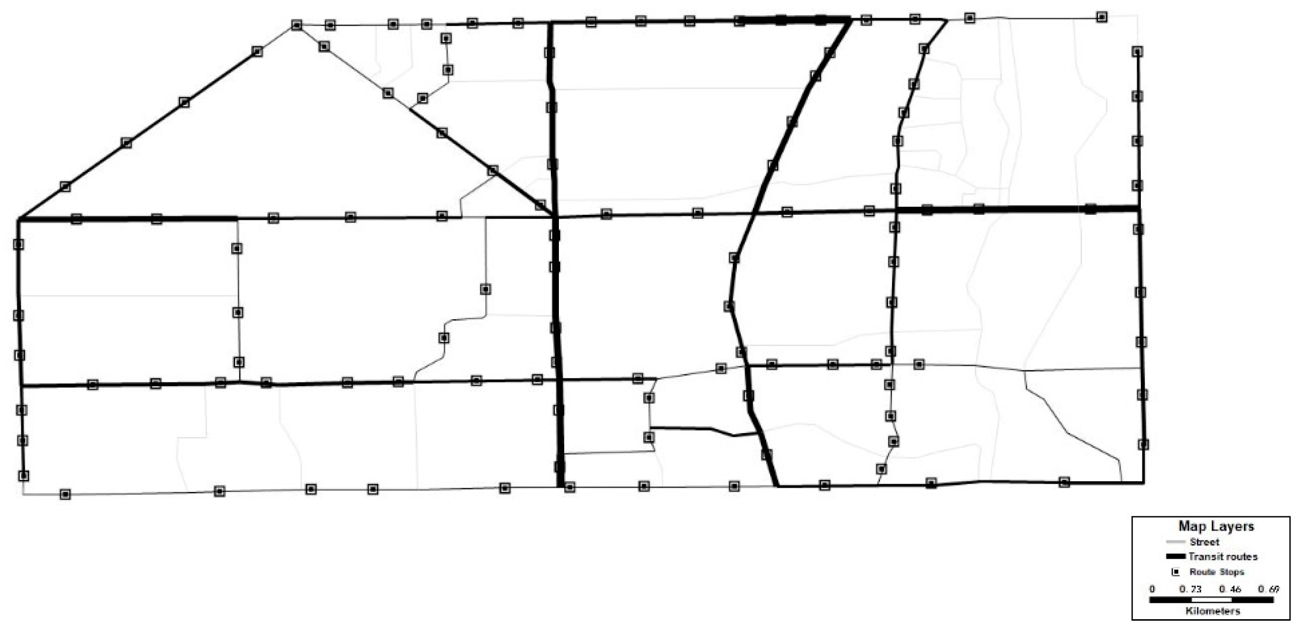
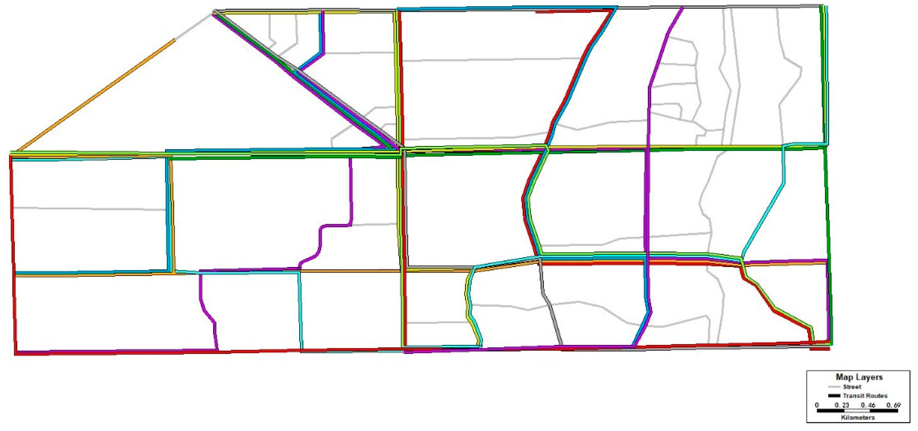
This paper selects the area enclosed by five roads including Yan’an Street, Ziyou Road, Linhe Street, Weixing Road and Qianjin Street in Nanguan District of Changchun City as examples to verify the feasibility of the optimization model and solution algorithm. The area covers about 20 square kilometers and is divided into 19 traffic zones. There are 3 rail transit routes, 19 conventional bus routes and 128 stations. The transit routes are shown in

Table 3. Direction of existing bus routes.

Number	Route Name	Approach Station
1	17	10-11-12-13-14-62-63-64-65-66-76-77-78-42-41-40-39-38
2	13	1-17-18-19-20-21-22-23-24-25-26
3	218	1-2-3-4-5-6-7-8-9-10-11-12-58-59-60-61-74-75-76-77-78
4	292	88-89-90-91-92-93-94-95-96-97-98-99-100-101
5	277	52-53-54-49-50-51-82-83-93-92-91-90-89-88
6	270	1-47-48-49-50-51-72-73-102-103-104-113-114
7	265	1-2-3-4-5-6-7-8-9-10-11-12-13-14-15-16
8	252	67-68-69-70-51-84-85-86-87-109-110
9	306	55-56-57-84-85-86-87-109-110
10	238	52-5-6-7-8-9-10-11-12-58-59-60-61-74-75-76-77-78-42-41-40-39-38
11	233	46-45-44-43-42-41-40-39-38
12	230	17-18-19-20-67-68-79-80-81-90
13	228	5-6-7-8-9-10-11-12-13-14-62-63-64-65-66-105-106-107-108-115-116-117-118
14	120	20-19-18-17-1-2-3-4-5-6-55-56-57-72-73-74-75-76-77-78-43-44-45-46
15	160	10-11-12-58-59-60-61-102-103-104-113-114-35-36-37
16	161	46-45-44-43-78-77-76-105-106-107-108-100-99-98-113-112-110
17	162	21-22-23-88-89-90-91-92-93-94-95-96-111-112-114-35-36-37
18	149	21-22-23-24-25-26-27-28-29-30-31
19	88	58-59-60-61-102-103-104-113-114-34-33-32

, and the OD matrix of the traffic zones is shown in

Table A1. OD matrix of the traffic zones.

	A	B	C	D	E	F	G	H	I	J	K	L	M	N	O	P	Q	R	S
A	0	663	452	642	426	290	160	941	317	725	769	210	238	199	346	349	561	253	261
B	730	0	864	645	584	321	282	921	365	751	756	356	498	369	698	864	235	854	621
C	498	448	0	839	759	417	367	1197	475	976	983	463	647	480	907	1123	306	1110	807
D	706	635	572	0	835	459	403	1317	522	1074	1081	509	712	528	998	1236	336	1221	888
E	768	691	622	560	0	551	484	1580	626	1289	1297	611	855	633	1198	1483	403	1465	1066
F	820	738	664	598	478	0	436	1422	564	1160	1168	550	769	570	1078	1334	363	1319	959
G	176	558	502	452	362	470	0	1280	507	1044	1051	495	692	513	970	1201	327	1187	863
H	1035	932	838	755	604	785	1020	0	609	1253	1261	594	831	615	1164	1441	392	1424	1036
I	349	314	283	254	204	265	344	310	0	354	132	245	234	351	254	124	120	140	78
G	798	368	331	298	238	310	403	363	435	0	1366	643	900	667	1261	1561	425	1543	1122
K	846	984	886	797	871	1132	1472	1325	1590	1749	0	579	810	600	1135	1405	382	1389	1010
L	231	208	187	168	135	175	228	205	246	270	243	0	683	596	402	372	508	829	930
M	268	741	667	600	480	624	811	730	876	964	868	621	0	477	321	297	407	664	744
N	219	742	668	601	481	625	813	731	878	965	869	542	488	0	418	387	529	863	967
O	381	543	489	440	352	457	595	535	642	706	636	365	329	394	0	348	476	776	870
P	384	346	311	280	224	291	378	341	409	450	405	338	304	365	345	0	381	621	696
Q	617	555	500	450	360	468	608	547	657	722	650	462	416	499	326	421	0	683	766
R	278	658	592	533	426	554	721	649	778	856	770	754	679	814	698	632	549	0	765
S	287	568	511	460	368	478	622	560	672	739	665	845	761	913	621	543	598	647	0

.

Road and transit routes are processed in order to obtain the road network and public transit network. The road network, traffic zones, station distribution and public transit network in the analysis area are shown in Figure 4, Figure 5 and Figure 6. The nodes in the road network are intersections, and the links are actual roads. The road network includes 77 nodes and 112 links; the nodes in the public transit network are stations, and the links are bus lines and transfer routes. The public transit network includes 128 nodes and 160 links.

For convenience of calculation, the following assumptions have been made in the application:

• The stopping time of each station is the same;
• The departure interval of all routes is the same;
• The waiting time of passengers on different paths is calculated according to the expected value;
• Transfer paths more than two are not considered;
• Combine upstream and downstream passenger flows to construct the network as an undirected network.

The origin and destination are determined by referring to the origin and destination of the existing bus routes. The parameter settings are shown in

Table 4. Parameter value of ant colony algorithm.

Parameter	Number of Stations	Number of Ants	Volatilization Coefficient	Number of Iterations
Value	128	100	0.9	100

and

Table 5. Constant value in optimization model.

Parameter	Departure Interval	Intersection Delay	Speed of Bus	Speed of Train	Stopping Time at Station	Transfer Penalty Coefficient
Value	8 min	30 s	15 km/h	80 km/h	15 s	1.2

.

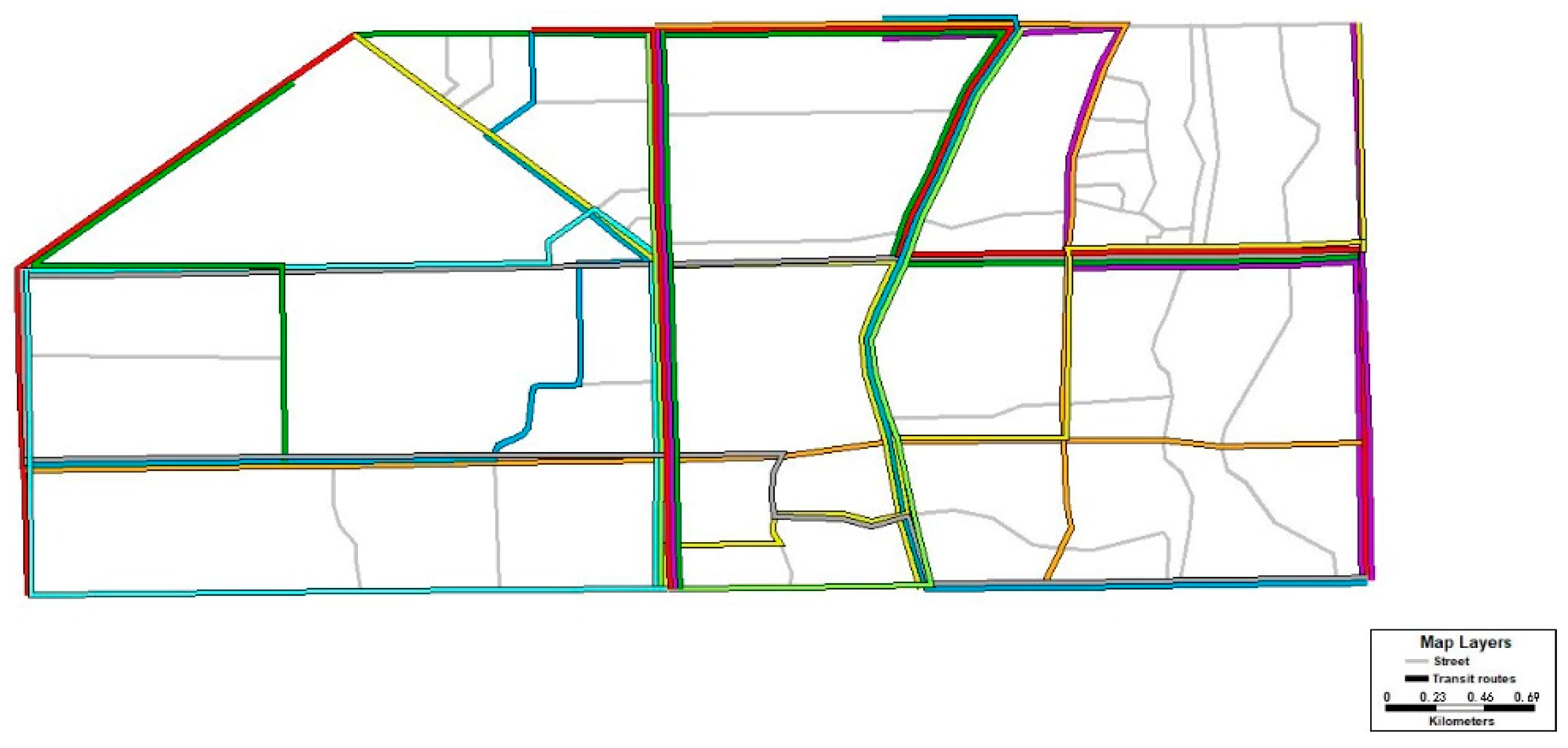
The optimal public transit network generated after iteration is shown in

Table 6. Direction of optimized bus routes.

Number	Route Name	Approach Station
1	17	10-11-12-58-59-60-61-74-75-76-77-121-122-123-124-37
2	13	1-47-48-49-50-51-82-83-93-92-125-126-28-27
3	218	1-47-48-49-50-51-72-73-74-75-76-77-78
4	292	88-89-90-91-92-93-94-95-96-97-98-99-100-101
5	277	52-53-54-49-50-51-71-70-69-79-80-81-90-89-88
6	270	1-2-3-4-5-6-55-56-57-84-85-86-87-96-111-112-34
7	265	1-2-3-4-5-6-7-8-9-10-11-12-13-14-15-16
8	252	67-68-79-80-81-91-125-126-29-30-31
9	306	55-56-57-84-85-86-87-109-110
10	238	52-53-54-49-50-51-72-73-74-75-105-106-107-108-101-39-38
11	233	46-45-44-43-42-41-40-39-38
12	230	17-18-19-20-67-68-79-80-81-90
13	228	5-6-7-8-9-10-11-12-58-59-60-61-103-104-98-99-100-115-116-117-118
14	120	67-68-69-70-71-72-73-74-75-76-77-78-43-44-45-46
15	160	10-11-12-58-59-60-61-102-103-104-113-114-35-36-37
16	161	46-45-44-43-78-121-122-101-100-99-98-97-111-112-33
17	162	67-68-69-70-71-72-73-102-103-104-98-99-100-101-123-124-37
18	149	21-22-23-24-25-26-27-28-29-30-31
19	88	58-59-60-61-102-103-104-97-111-112-33-32

and Figure 7. Some network evaluation indicators are selected and compared with the original public transit network, and the specific indicator calculation results are shown in

Table 7. Comparison of indicators before and after optimization (network).

Indicator	Value before Optimization	Value after Optimization
Average impedance	35.94	32.25
Network efficiency	0.18669	0.20253

and

Table 8. Comparison of indicators before and after optimization (routes).

Number	Route Name	Existing Bus Routes		Optimized Bus Routes
		Length (km)	Non-Linear Coefficient	Length (km)	Non-Linear Coefficient
1	17	6	1.2	5.7	1.1
2	13	4.5	1	6.3	1.4
3	218	6.6	1.3	5.2	1
4	292	6	1	6	1
5	277	6.2	1.4	6	1.4
6	270	5.2	1	6.1	1.2
7	265	4.5	1	4.5	1
8	252	4.9	1	4.9	1
9	306	3.9	1	3.9	1
10	238	7.9	1.2	7.1	1.1
11	233	3.5	1	3.5	1
12	230	4	1	4	1
13	228	5.7	1	6	1.1
14	120	9.5	1.4	7.5	1.1
15	160	8.6	1.3	7.2	1.1
16	161	6.6	1	6.3	1
17	162	7.9	1	7.7	1
18	149	4.9	1	4.9	1
19	88	4.8	1.2	4.5	1.1

.

After optimization, network efficiency and average impedance are 0.20253 and 32.25, respectively, and original network efficiency and average impedance are 0.18669 and 35.94, respectively. Before optimization, there were 23 links where saturation was greater than 1 in the network, the maximum value was 1.99 and the minimum value was 0.06; after optimization, there were eight links in which saturation was greater than 1 in the network, the maximum value was 1.92 and the minimum value was 0.15. Comparing Figure 6 and Figure 7, the distribution of optimized bus routes on the road network is more balanced. Comparing Table 3 and Table 6, all bus routes except 292, 265, 252, 306, 233, and 230 have obvious changes. After optimization, the average non-linear coefficient of the bus route decreases, network efficiency increases and average impedance decreases. Based on the above analysis, establishing the optimization model to improve network efficiency and the use of an ant colony algorithm to realize optimal transit network planning can improve the operating efficiency of the network.

4. Discussion

This paper presents an urban public transit network optimization model. Firstly, passenger travel cost is calculated and added to the network as the travel impedance, and then the probability of passengers choosing the travel path is calculated according to travel impedance. The passenger demand of different sections can be obtained. Travel impedance, passenger demand and passenger capacity of public transit are added to the transit network as weights, and the calculation method of network efficiency is improved according to the weights. Finally, a public transit network optimization model is established with the network efficiency as the objective function, and the ant colony algorithm was improved to solve it. Example analysis shows that the global efficiency of the transit network solved by the optimization model is improved, passenger travel impedance is reduced and passenger travel demand and capacity are more balanced.

Compared with the traditional transit network optimization method, the optimization method in this paper not only considers traditional indicators such as passenger demand, route length and non-linear coefficient but also considers the overall operation efficiency of the network, reduces the average travel impedance of passengers and alleviates the imbalance between supply and demand. The disadvantage of this paper is that passenger travel impedance only considers time cost, without considering the factors such as money cost and comfort. Passenger travel demand data are allocated by traditional methods, and real bus travel data are more representative. Only pedestrian transfer is considered when considering the transfer process, but shared bicycle, public bicycle and P + R modes expand the scope of passengers’ choice of bus routes, and it is necessary to further explore the impact of different transfer modes on the network.

References

- Tian, G.; Liu, X.; Zhang, M.; Yang, Y.; Zhang, H.; Lin, Y.; Ma, F.; Wang, X.; Qu, T.; Li, Z. Selection of take-back pattern of vehicle reverse logistics in China via Grey-DEMATEL and Fuzzy-VIKOR combined method. J. Clean. Prod. 2019, 220, 1088–1100. [Google Scholar] [CrossRef]
- Li, Z.; Li, Q.; Sun, Y.; Li, H.; Yao, L.; Shi, Y.; You, X. A study on the research status quo of sustainable preferential development of public transportation in large and medium-sized cites. J. Beijing Jiaotong Univ. 2013, 12, 37–46, 51. [Google Scholar]
- Fathollahi-Fard, A.M.; Hajiaghaei-Keshteli, M.; Tian, G.; Li, Z. An adaptive Lagrangian relaxation-based algorithm for a coordinated water supply and wastewater collection network design problem. Inf. Sci. 2020, 512, 1335–1359. [Google Scholar] [CrossRef]
- Tian, G.; Feng, Y.; Zhou, M.; Zhang, H.; Tan, J. Modeling and Planning for Dual-Objective Selective Disassembly Using AND/OR Graph and Discrete Artificial Bee Colony. IEEE Trans. Ind. Inform. 2019, 15, 2456–2468. [Google Scholar] [CrossRef]
- Li, C. Research on Connectivity of Urban Transit Network Based on Theory of Complex Network. Master’s Thesis, Southwest Jiaotong University, Chengdu, China, 2014. [Google Scholar]
- Amaral, L.A.N.; Scala, A.; Barthelemy, M.; Stanley, H.E. Classes of small-world networks. Proc. Natl. Acad. Sci. USA 2000, 97, 11149–11152. [Google Scholar] [CrossRef] [Green Version]
- Sienkiewicz, J.; Hołyst, J.A. Statistical analysis of 22 public transport networks in Poland. Phys. Rev. E 2005, 72 Pt 2, 046127. [Google Scholar] [CrossRef] [PubMed] [Green Version]
- Yang, J.; Li, Z. Analysis of survivability of urban rail transit network based on passenger flow weighting. Sci. Technol. Innov. 2017, 6, 1–4. [Google Scholar]
- Lu, Q.; Cui, X.; Xu, B.; Liu, P.; Wang, Y. Vulnerability research of rail transit network under bus connection scenarios. China Saf. Sci. J. 2021, 31, 141–146. [Google Scholar]
- Zhou, Y. Design and research on weighted network of urban intelligent public transportation system based on internet of things —Take Wuhan as an example. Mod. Inf. Technol. 2019, 3, 170–171. [Google Scholar]
- Cats, O.; Koppenol, G.J.; Warnier, M. Robustness assessment of link capacity reduction for complex networks: Application for public transport systems. Reliab. Eng. Syst. Saf. 2017, 167, 544–553. [Google Scholar] [CrossRef] [Green Version]
- Ding, J.; Zhong, Y.; Li, B.; Zhang, S. Study on public transit network optimization based on improved K-shortest path algorithm. J. Hefei Univ. Technol. 2019, 42, 1388–1393, 1423. [Google Scholar]
- Lu, H.; Chen, L.; Zhang, Z.; Xu, K. Research on optimization method of conventional bus routes alongside rail transit. Technol. Method 2018, 37, 54–59. [Google Scholar]
- Wang, F. Research on Characteristic Analysis and Optimization of Transit Network Based on Complex Network Theory. Master’s Thesis, Beijing Jiaotong University, Beijing, China, 2020. [Google Scholar]
- Hao, Y. Urban Multimodal Bus Network Optimization Based on Accessibility. Master’s Thesis, Chang’an University, Xi’an, China, 2019. [Google Scholar]
- Zhou, X. The Analysis of Weighted Composite Network Model and Robustness of Nanjing Bus and Subway Network. Master’s Thesis, Nanjing University of Posts and Telecommunications, Nanjing, China, 2016. [Google Scholar]
- Peng, J. Modeling and Empirical Analysis of Bus and Subway Weighted Composite Network in Nanjing. Master’s Thesis, Nanjing University of Posts and Telecommunications, Nanjing, China, 2017. [Google Scholar]
- Lai, Q.; Zhang, H.; Wang, X. Robustness analysis and optimization of urban public transport network based on complex network theory. Comput. Eng. Appl. 2021. Available online: http://kns.cnki.net/kcms/detail/11.2127.TP.20210224.1049.010.html (accessed on 8 November 2021).
- Cao, Z.; Jiang, S.; Luo, X.; Yang, J.; Zhang, Y. A Direct Optimization in Urban Transit Network for Small and Medium-sized Cities. Ind. Eng. J. 2020, 23, 117–123. [Google Scholar]
- Cheng, X. Research on Cooperative Optimization and Cascading Failure Evolution of Metro-Bus Network Based on Double-layer Coupling Network. Master’s Thesis, Lanzhou Jiaotong University, Lanzhou, China, 2020. [Google Scholar]
- Tian, G.; Zhou, M.; Li, P.; Zhang, C.; Jia, H. Multiobjective Optimization Models for Locating Vehicle Inspection Stations Subject to Stochastic Demand, Varying Velocity and Regional Constraints. IEEE Trans. Intell. Transp. Syst. 2016, 17, 1978–1987. [Google Scholar] [CrossRef]
- Latora, V.; Marchiori, M. Is the Boston subway a small-world network? Phys. A Stat. Mech. Its Appl. 2002, 314, 109–113. [Google Scholar] [CrossRef] [Green Version]
- Luo, Y.; Qian, D. Research of weight adjustment on the efficiency of transit networks. J. Beijing Jiaotong Univ. 2018, 3, 170–171. [Google Scholar]
- Tian, G.; Chu, J.; Liu, Y.; Ke, H.; Zhao, X.; Xu, G. Expected energy analysis for industrial process planning problem with fuzzy time parameters. Comput. Chem. Eng. 2011, 35, 2905–2912. [Google Scholar] [CrossRef]
Figure 1.
Schematic diagram of passenger route selection.
Figure 2.
Ant colony algorithm solution.
Figure 3.
(a) Theoretical road network and station; (b) the result of the original optimization method; (c) the result of the improved optimization method.
Figure 4.
Road network and traffic zones division.
Figure 5.
Bus stations and transit network.
Figure 6.
Schematic diagram of transit routes.
Figure 7.
Optimized transit network.