A Dynamically Adjusted Subspace Gradient Method and Its Application in Image Restoration

Abstract

In this paper, a new subspace gradient method is proposed in which the search direction is determined by solving an approximate quadratic model in which a simple symmetric matrix is used to estimate the Hessian matrix in a three-dimensional subspace. The obtained algorithm has the ability to automatically adjust the search direction according to the feedback from experiments. Under some mild assumptions, we use the generalized line search with non-monotonicity to obtain remarkable results, which not only establishes the global convergence of the algorithm for general functions, but also R-linear convergence for uniformly convex functions is further proved. The numerical performance for both the traditional test functions and image restoration problems show that the proposed algorithm is efficient.

1. Introduction

The Conjugate Gradient (CG) method is dedicated to solving the unconstrained optimization problem:

$$\underset{x\in {\Re }^n}{min}f\left(x\right),$$

(1)

where $f:R^n\to R$ is smooth and the gradient of $f\left(x\right)$ at $x_k$ is marked $g_k$. The advantages of its simple form and low storage requirements make the CG method a powerful tool for dealing with problem (1). It starts at a starting point $x_0$ and generates an iterative sequence $\left\{x_k\right\}$ in the following form:

$$x_{k+1}=x_k+{\alpha }_k{d}_k,k\ge 0,$$

(2)

that is, $x_k$ moves forward by one step ${\alpha }_k$ along the search direction $d_k$ and reaches the $(k+1)$-th iteration point $x_{k+1}$.

The direction $d_k$ is usually defined as

$$d_k=\left\{\begin{array}{cc}-g_k,\hfill & \mathrm{if}k=0,\hfill \\ -g_k+{\beta }_k{d}_{k-1},\hfill & \mathrm{if}k\ge 1,\hfill \end{array}\right.$$

(3)

where ${\beta }_k$ is CG parameter. The different ${\beta }_k$ corresponds to different CG methods, such as Polak and Ribiere (PRP) [1], Hestenes and Stiefel (HS) [2], Liu and Storey (LS) [3], Fletcher and Reeves (FR) [4], Dai and Yuan (DY) [5], and the conjugate descent (CD) method [6]. In addition, more relevant research and the progress of CG method can be found in the literature [7,8,9,10].

The step size ${\alpha }_k$ can be obtained by different rules. In this paper, we focus on the following generalized line search, which has been shown to be very efficient for CG methods in [11].

$$\begin{array}{c}\hfill \begin{array}{cc}& f(x_k+{\alpha }_k{d}_k)\le C_k+\delta {\alpha }_k{g}_k^T{d}_k,\hfill \\ & g_{k+1}^T{d}_k\ge \sigma g_k^T{d}_k,\hfill \end{array}\end{array}$$

(4)

where the definition of $C_k$ is as follows:

$$C_0=f\left(x_0\right),Q_0=1,Q_{k+1}=Q_k+1,C_{k+1}=\frac{Q_k{C}_k+f_{k+1}}{Q_{k+1}}.$$

(5)

From Equation (5), we can find that $C_k$ is a convex combination of the function values $f\left(x_0\right)$ to $f\left(x_k\right)$. The generalized line search is non-monotonic, which facilitates the establishment of the global convergence of the algorithm under milder conditions.

Subspace technology plays an extraordinary role in solving large-scale unconstrained optimization problems. As the scale of optimization problems to be dealt with continues to expand, subspace technology has attracted increased attention from researchers. Using subspace minimization technology with CG method, Yuan and Stoer [12] creatively proposed theSMCG method, in which the approximate function of $f\left(x\right)$ is minimized on the subspace ${\Omega }_{k+1}=Span\{g_{k+1},s_k\}$, and the expression of the search direction is derived:

$$d_{k+1}={\mu }_k{g}_{k+1}+{\nu }_k{s}_k,$$

(6)

where ${\mu }_k$ and ${\nu }_k$ are parameters, and $s_k=x_{k+1}-x_k$. Obviously, the SMCG method is a further promotion based on the CG method, and at the same time, it has a profound influence on the subsequent vigorous development of subspace technology. Based on Yuan’s ideas above, Andrei [13] developed a new SMCG method, in which it further expands the search direction, develops into three subspaces, and used the acceleration strategy. Inspired by Andrei, Yang et al. [14] applied the technique of subspace minimization to another special three-term subspace and came up with a new SMCG method. On the same subspace, Li et al. [10] conducted a more in-depth study of Yang’s results, analyzed more complex three-parameter situations, and set different conditions to dynamically select the search direction under different dimensions of subspace. Subspace technology has more extensive applications. Dai [15] proposed a new method called BBCG by fusing it with the Barzilai–Borwein [16] method and compared the performance of several BBCG methods proposed in the article through numerical experiments. It was found that the BBCG3 method has better performance. Many scholars have also tried to integrate the idea of minimizing subspace into the trust region method. For related research, readers can refer to [17]. More research on the use of subspace technology to construct different methods is still in progress [18,19,20,21,22].

The outline of this article is as follows: in Section 2, we give preliminary information. In Section 3, the search direction is be discussed first, and then the obtained algorithm is proposed. Based on the above-mentioned work, under some mild assumptions, the global convergence of the algorithm for general functions is proved; more importantly, the result of R-linear convergence for uniformly convex functions is also established. Some numerical results for solving unconstrained opitmization problems and image restoration problems are shown in Section 4. The conclusion and discussion are presented in Section 5.

2. Preliminary

The main work of this section is: in the subspace ${\Omega }_{k+1}=Span\{-g_{k+1},s_k,g_k\}$, according to the different dimensions of ${\Omega }_{k+1}$, the discussion is divided into three cases; then, combined with the technique of subspace minimization, four forms of $d_k$ are determined, and the conditions for dynamic selection of each direction are given.

In this paper, the direction at $x_{k+1}$ is expected to minimize the quadratic approximation of the objective function,

$$\underset{d\in {\Omega }_{k+1}}{min}{\varphi }_{k+1}\left(d\right)=g_{k+1}^{T}d+\frac{1}{2}{d}^T{B}_{k+1}d,$$

(7)

on the subspace ${\Omega }_{k+1}$, where $B_{k+1}$ is regarded as an approximation of the Hessian matrix and is positive definite. Assuming $B_{k+1}$ satisfies the modified secant equation [23]

$$B_{k+1}{s}_k=y_k^{*}=y_k+\frac{max\{z_k,0\}}{s_k^T{s}_k}{s}_k,$$

(8)

where $z_k=2(f_k-f_{k+1})+{(g_{k+1}+g_k)}^T{s}_k$. Combined with (4), obviously, $s_k^T{y}_k^{*}\ge s_k^T{y}_k>0$.

3. Proposed Method

3.1. Direction Selection

According to the above discussion, as is known, the subspace may have three different dimensions; based on that, we analyze the selection of the search direction in the next section.

Case I: dim(${\Omega }_{k+1}$) = 3.

In this case, the direction can be expressed as

$$d_{k+1}=a_k{g}_{k+1}+b_k{s}_k+c_k{g}_k,$$

(9)

where $a_k,b_k,c_k$ are parameters to be determined. Substituting (9) into (7), we get

$$\{a_k,b_k,c_k\}=\underset{(a,b,c)}{argmin}{\left(\begin{array}{c}\Vert g_{k+1}{\Vert }^2\\ g_{k+1}^T{s}_k\\ g_{k+1}^T{g}_k\end{array}\right)}^T\left(\begin{array}{c}a\\ b\\ c\end{array}\right)+\frac{1}{2}{\left(\begin{array}{c}a\\ b\\ c\end{array}\right)}^T\left(\begin{array}{ccc}{\rho }_{k+1}& g_{k+1}^T{y}_k^{*}& w_k\\ g_{k+1}^T{y}_k^{*}& s_k^T{y}_k^{*}& g_k^T{y}_k^{*}\\ w_k& g_k^T{y}_k^{*}& {\rho }_k\end{array}\right)\left(\begin{array}{c}a\\ b\\ c\end{array}\right),$$

(10)

where ${\rho }_k=g_k^T{B}_{k+1}{g}_k$, ${\rho }_{k+1}=g_{k+1}^T{B}_{k+1}{g}_{k+1}$, $w_k=g_{k+1}^T{B}_{k+1}{g}_k$. Inspired by the BBCG method [11], we set

$$w_k={\xi }_k\frac{g_{k+1}^T{g}_k{\Vert y_k\Vert }^2}{s_k^T{y}_k},{\xi }_k=\left\{\begin{array}{cc}max\{0.9{\xi }_{k-1},1.2\},\hfill & if{\alpha }_k>1,\hfill \\ min\{1.1{\xi }_{k-1},1.75\},\hfill & otherwise,\hfill \end{array}\right.$$

(11)

where ${\xi }_k$ is an adaptive parameter, and its value remains the same throughout the whole paper. Setting ${\xi }_0=1.5$, we not only find that $1.2\le {\xi }_k\le 1.75$, but we also show that its numerical performance is better than a constant. The matrix in (10) is represented by $D_k$.

The positive definiteness of $D_k$ is presented in Lemma 1. Now that we assume that $D_k$ is positive definite, the unique solution of (10) can be calculated as follows:

$$\left(\begin{array}{c}{a}_k\\ b_k\\ c_k\end{array}\right)=-\frac{1}{{▵}_k}\left(\begin{array}{ccc}\chi & {\theta }_1& {\theta }_2\\ {\theta }_1& \theta & {\theta }_3\\ {\theta }_2& {\theta }_3& \nu \end{array}\right)\left(\begin{array}{c}\Vert g_{k+1}{\Vert }^2\\ g_{k+1}^T{s}_k\\ g_{k+1}^T{g}_k\end{array}\right),$$

(12)

where

• ${▵}_k=\left|D_k\right|={\rho }_{k+1}\chi +w_k{\theta }_2+g_{k+1}^T{y}_k^{*}{\theta }_1$,
• $\chi ={\rho }_k\left(s_k^T{y}_k^{*}\right)-{\left(g_k^T{y}_k^{*}\right)}^2$,
• $\nu ={\rho }_{k+1}\left(s_k^T{y}_k^{*}\right)-{\left(g_{k+1}^T{y}_k^{*}\right)}^2$,
• ${\theta }_3=w_k\left(g_{k+1}^T{y}_k^{*}\right)-{\rho }_{k+1}\left(g_k^T{y}_k^{*}\right)$,
• ${\theta }_1=w_k\left(g_k^T{y}_k^{*}\right)-{\rho }_k\left(g_{k+1}^T{y}_k^{*}\right)$,
• $\theta ={\rho }_k{\rho }_{k+1}-{\left(w_k\right)}^2$,
• ${\theta }_2=\left(g_k^T{y}_k^{*}\right)\left(g_{k+1}^T{y}_k^{*}\right)-w_k\left(s_k^T{y}_k^{*}\right)$.

If $D_k$ is positive definite, then ${▵}_k>0$, so

$${\rho }_{k+1}\ge \frac{-w_k{\theta }_2-g_{k+1}^T{y}_k^{*}{\theta }_1}{\chi }=h_k.$$

(13)

Setting $n_k=1-\frac{{\left(g_k^T{y}_k^{*}\right)}^2}{{\rho }_k\left(s_k^T{y}_k^{*}\right)}$ and substituting the variable value in Equation (12), we get

$$\begin{array}{cc}\hfill & \chi =n_k{\rho }_k\left(s_k^T{y}_k^{*}\right),\hfill \\ \hfill & h_k=\frac{(\frac{w_k^2}{{\rho }_k}+\frac{{\left(g_{k+1}^T{y}_k^{*}\right)}^2}{s_k^T{y}_k^{*}}-\frac{2w_k\left(g_{k+1}^T{y}_k^{*}\right)\left(g_k^T{y}_k^{*}\right)}{{\rho }_k\left(s_k^T{y}_k^{*}\right)})}{n_k}.\hfill \end{array}$$

(14)

Considering the formula in Equation (13), we compute ${\rho }_{k+1}$ as

$${\rho }_{k+1}={\xi }_{k}max\{h_k,N\},$$

(15)

where $N=N_1{\Vert g_{k+1}\Vert }^2$, $N_1=max\{\frac{\Vert y_k^{*}{\Vert }^2}{s_k^T{y}_k^{*}},\frac{4\Vert y_k^{*}{\Vert }^4{\Vert g_k^{*}\Vert }^2}{{\rho }_k{\left(s_k^T{y}_k^{*}\right)}^2}\}$.

In order to make the algorithm perform better, in a manner similar to [7,24], we set the following conditions:

$${\rho }_0\le n_k,$$

(16)

$${\zeta }_1\le \frac{s_k^T{y}_k}{\Vert s_k{\Vert }^2}\le \frac{\Vert y_k^{*}{\Vert }^2}{s_k^T{y}_k^{*}}\le {\zeta }_2,$$

(17)

$${\zeta }_1\le \frac{{\rho }_k}{\Vert g_k{\Vert }^2},\frac{4\Vert y_k^{*}{\Vert }^4{\Vert g_k^{*}\Vert }^2}{{\rho }_k{\left(s_k^T{y}_k^{*}\right)}^2}\le {\zeta }_2,$$

(18)

where ${\zeta }_1,{\zeta }_2$ are positive constants, ${\rho }_0\in (0,1)$.

Now, we prove that $D_k$ is positive definite.

Lemma 1.

If ${\rho }_{k+1}$ is calculated by Equation (15), then the matrix $D_k$ is positive definite.

Proof. 

Using mathematical induction and ${\rho }_0\in (0,1)$, we can get ${\rho }_{k+1}\ge {\xi }_{k}N>0$; because ${\rho }_{k+1}>\frac{\Vert g_{k+1}{\Vert }^2{\Vert y_k^{*}\Vert }^2}{s_k^T{y}_k^{*}}$, so $\nu ={\rho }_{k+1}\left(s_k^T{y}_k^{*}\right)-{\left(g_{k+1}^T{y}_k^{*}\right)}^2>0$; since ${\rho }_{k+1}>h_k=\frac{-w_k{\theta }_2-g_{k+1}^T{y}_k^{*}{\theta }_1}{\chi }$, therefore ${▵}_k=\left|D_k\right|={\rho }_{k+1}\chi +w_k{\theta }_2+g_{k+1}^T{y}_k^{*}{\theta }_1>0$. □

Case II: dim(${\Omega }_{k+1}$) = 2.

We define $d_k$ as

$$d_{k+1}=a_k{g}_{k+1}+b_k{s}_k,$$

(19)

where $a_k,b_k$ are parameters. Similarly, substituting Equation (19) into the approximation function (7), we find

$$\{a_k,b_k\}=\underset{(a,b)}{argmin}{\left(\begin{array}{c}\Vert g_{k+1}{\Vert }^2\\ g_{k+1}^T{s}_k\end{array}\right)}^T\left(\begin{array}{c}a\\ b\end{array}\right)+\frac{1}{2}{\left(\begin{array}{c}a\\ b\end{array}\right)}^T\left(\begin{array}{cc}{\rho }_{k+1}& g_{k+1}^T{y}_k^{*}\\ g_{k+1}^T{y}_k^{*}& s_k^T{y}_k^{*}\end{array}\right)\left(\begin{array}{c}a\\ b\end{array}\right).$$

(20)

If ${▵}_k={\rho }_{k+1}\left(s_k^T{y}_k^{*}\right)-{\left(g_{k+1}^T{y}_k^{*}\right)}^2>0$, then Equation (20) has a unique solution:

$$\left(\begin{array}{c}{a}_k\\ b_k\end{array}\right)=\frac{1}{{▵}_k}\left(\begin{array}{c}\left(g_{k+1}^T{y}_k^{*}\right)\left(g_{k+1}^T{s}_k\right)-\left(s_k^T{y}_k^{*}\right){\Vert g_{k+1}\Vert }^2\\ \left(g_{k+1}^T{y}_k^{*}\right){\Vert g_{k+1}\Vert }^2-{\rho }_{k+1}\left(g_{k+1}^T{s}_k\right)\end{array}\right).$$

(21)

Similar to the way that Equation $w_k$ in (11) is evaluated, we set ${\rho }_{k+1}={\xi }_k\frac{\Vert g_{k+1}{\Vert }^2{\Vert y_k^{*}\Vert }^2}{s_k^T{y}_k^{*}}$; apparently, ${▵}_k>0$. Furthermore, for the better performance of the algorithm, we require relevant variables to satisfy the condition in Equation (17).

As we all know, DY and HS methods have some good properties. For example, the finite termination of HS is helpful to improve the convergence rate. In view of the above considerations, we put forward an idea; when the conditions

$${\zeta }_1\le \frac{s_k^T{y}_k}{\Vert s_k{\Vert }^2},\frac{\Vert g_{k+1}\Vert \Vert d_k\Vert }{d_k^T{y}_k}\le {\zeta }_3,$$

(22)

$$\frac{|g_{k+1}^T{y}_k{g}_{k+1}^T{d}_k|}{d_k^T{y}_k{\Vert g_{k+1}\Vert }^2}\le {\zeta }_3,$$

(23)

are met, we take

$$d_{k+1}=-g_{k+1}+{\beta }_k{d}_k,{\beta }_k=max\{{\beta }_k^{HS},{\beta }_k^{DY}\},$$

(24)

where ${\zeta }_3\in [0,1)$.

Above all, in the case of two-dimensional subspace, when the condition (17) is established, $d_k$ takes Equations (19) and (21); when the inequalities in Equations (22) and (23) are true, $d_k$ is calculated by Equation (24).

Case III: dim(${\Omega }_{k+1}$) = 1.

When dim(${\Omega }_{k+1}$) = 1, we adopt the method of the steepest descent, namely $d_{k+1}=-g_{k+1}$.

3.2. Description of DSCG Algorithm

In this section, we first introduce an acceleration strategy (Algorithm 1) [25] which has been shown to be quite efficient for the CG method. Then, we present our dynamically adjusted subspace conjugate gradient algorithm (DSCG, Algorithm 2) and prove that the direction satisfies sufficient descent.

Algorithm 1: Acceleration Strategy.

Step 1: Compute: $z=x_k+{\alpha }_k{d}_k,g_z=\nabla f\left(z\right)$ and $y_z=g_k-g_z$; Step 2: Compute: ${\overline{a}}_k={\alpha }_k{g}_k^T{d}_k$ and ${\overline{b}}_k=-{\alpha }_k{y}_k^T{d}_k$; Step 3: If ${\overline{b}}_k>0$, then, compute ${\eta }_k=-\frac{{\overline{a}}_k}{{\overline{b}}_k}$ and update the variables as $x_{k+1}=x_k+{\eta }_k{\alpha }_k{d}_k$, otherwise update the variables as $x_{k+1}=x_k+{\alpha }_k{d}_k$.

Algorithm 2: DSCG.

Step 1: Given $x_0\in {\Re }^n$, ${\alpha }_0^{\left(0\right)}$, $ϵ>0$, ${\zeta }_1$,${\zeta }_2$,${\zeta }_3\in [0,1)$. Let $d_0:=-g_0$ and $k:=0$. Step 2: When $\Vert g_k\Vert \le ϵ$, stop, otherwise go to step 3. Step 3: Compute a stepsize ${\alpha }_k$ that satisfies conditions (4) and (5), then adopt Algorithm 1 (acceleration strategy). Step 4: Compute the direction $d_k$. Step 4.1: If the conditions (17) holds, compute $d_{k+1}$ by Equations (19) and (21), and go to Step 5; Step 4.2: If the conditions (22) and (23) holds, compute $d_{k+1}$ by Equation (24), and go to Step 5; Step 4.3: If the conditions (16)–(18) hold, compute $d_{k+1}$ by Equations (9) and (12), and go to Step 5; Step 4.4: Otherwise, set $d_{k+1}=-g_{k+1}$. Step 5: Set $k:=k+1$, and go to step 2.

3.3. Convergence Analysis

In this subsection, we focus on the convergence properties of the proposed algorithm (DSCG). The sufficient descent condition is crucial for a gradient descent algorithm. In order to establish the sufficient descent condition for the DSCG method, we firstly introduce the following lemma.

Lemma 2.

If $d_{k+1}$ is generated by Equations (9) and (12) or by Equations (19) and (20), then

$$g_{k+1}^T{d}_{k+1}\le -\frac{\Vert g_{k+1}{\Vert }^4}{{\rho }_{k+1}},$$

(25)

holds.

Proof. 

If $d_{k+1}$ is generated by Equations (19) and (20), we get

$$\begin{array}{c}\hfill \begin{array}{cc}\hfill g_{k+1}^T{d}_{k+1}& =-\frac{\Vert g_{k+1}{\Vert }^4}{{▵}_k}[s_k^T{y}_k^{*}-2\frac{\left(g_{k+1}^T{y}_k^{*}\right)\left(g_{k+1}^T{s}_k\right)}{\Vert g_{k+1}{\Vert }^2}+{\rho }_{k+1}{\left(\frac{g_{k+1}^T{s}_k}{\Vert g_{k+1}{\Vert }^2}\right)}^2]\hfill \\ & \le -\frac{\Vert g_{k+1}{\Vert }^4}{{▵}_k}{H}_{min}\left(\frac{g_{k+1}^T{s}_k}{\Vert g_{k+1}{\Vert }^2}\right)\hfill \\ & =-\frac{\Vert g_{k+1}{\Vert }^4}{{▵}_k}H\left(\frac{g_{k+1}^T{y}_k^{*}}{{\rho }_{k+1}}\right)\hfill \\ & =-\frac{\Vert g_{k+1}{\Vert }^4}{{▵}_k}\frac{{▵}_k}{{\rho }_{k+1}}\hfill \\ & =-\frac{\Vert g_{k+1}{\Vert }^4}{{\rho }_{k+1}},\hfill \end{array}\end{array}$$

(26)

where $H_{min}\left(\frac{g_{k+1}^T{s}_k}{\Vert g_{k+1}{\Vert }^2}\right)$ represents the minimum value of function $s_k^T{y}_k^{*}-2\frac{\left(g_{k+1}^T{y}_k^{*}\right)\left(g_{k+1}^T{s}_k\right)}{\Vert g_{k+1}{\Vert }^2}+{\rho }_{k+1}{\left(\frac{g_{k+1}^T{s}_k}{\Vert g_{k+1}{\Vert }^2}\right)}^2$ with $\frac{g_{k+1}^T{s}_k}{\Vert g_{k+1}{\Vert }^2}$ as the variable.

When $d_{k+1}$ is given by Equations (9) and (12),

$$\begin{array}{c}\hfill \begin{array}{cc}\hfill g_{k+1}^T{d}_{k+1}& ={\left(\begin{array}{c}\Vert g_{k+1}{\Vert }^2\\ g_{k+1}^T{s}_k\\ g_{k+1}^T{g}_k\end{array}\right)}^T\left(\begin{array}{c}a\\ b\\ c\end{array}\right)\hfill \\ & =-\frac{1}{{▵}_k}\left(\begin{array}{c}\Vert g_{k+1}{\Vert }^2\\ g_{k+1}^T{s}_k\\ g_{k+1}^T{g}_k\end{array}\right)\left(\begin{array}{ccc}\chi & {\theta }_1& {\theta }_2\\ {\theta }_1& \theta & {\theta }_3\\ {\theta }_2& {\theta }_3& \nu \end{array}\right)\left(\begin{array}{c}\Vert g_{k+1}{\Vert }^2\\ g_{k+1}^T{s}_k\\ g_{k+1}^T{g}_k\end{array}\right)\hfill \\ & =-\frac{\Vert g_{k+1}{\Vert }^4}{{▵}_k}\phi (x,y),\hfill \end{array}\end{array}$$

(27)

taking $x=\frac{g_{k+1}^T{g}_k}{\Vert g_{k+1}{\Vert }^2},y=\frac{g_{k+1}^T{s}_k}{\Vert g_{k+1}{\Vert }^2}$ as independent variable, where $\phi (x,y)=\nu x^2+2{\theta }_{3}xy+\theta y^2+2{\theta }_{2}x+2{\theta }_{1}y+\chi$.

From Lemma 1, we find that $\nu >0$, $\nu \theta -{\theta }_3^2={▵}_k{\rho }_{k+1}>0$; that is, there is a minimum value for $\phi (x,y)$, which is calculated to be $\phi {(x,y)}_{min}=\frac{{▵}_k}{{\rho }_{k+1}}$.

Therefore, we can also get $g_{k+1}^T{d}_{k+1}\le -\frac{\Vert g_{k+1}{\Vert }^4}{{\rho }_{k+1}}$. □

Lemma 3.

Suppose $d_{k+1}$ is generated by the DSCG algorithm. Then, there is a constant $c_3>0$, such that

$$g_{k+1}^T{d}_{k+1}\le -c_3{\Vert g_{k+1}\Vert }^2.$$

(28)

Proof. 

Based on the form of direction, we analyze this in three cases:

Case I: if $d_{k+1}=-g_{k+1}$, let $c_3=\frac{1}{2}$, and thus it is proved.

Case II: When the direction is binomial, the following information must be considered.

We first discuss the case where $d_{k+1}$ is given by Equations (19) and (21); here, for ${\rho }_{k+1}={\xi }_k\frac{\Vert g_{k+1}{\Vert }^2{\Vert y_k^{*}\Vert }^2}{s_k^T{y}_k^{*}}$, combined with the conditions (11), (17) and Lemma 2, the following results can be obtained:

$${\rho }_{k+1}\le 2{\zeta }_2\Vert g_{k+1}{\Vert }^2,g_{k+1}^T{d}_{k+1}\le -\frac{1}{2{\zeta }_2}{\Vert g_{k+1}\Vert }^2.$$

(29)

When $d_k$ is determined by Equation (24), for ${\beta }_k={\beta }_k^{DY}$, we have

$$\begin{array}{c}\hfill \begin{array}{cc}\hfill g_{k+1}^T{d}_{k+1}& =-\Vert g_{k+1}{\Vert }^2+{\beta }_k{g}_{k+1}^T{d}_k\hfill \\ & \le -\Vert g_{k+1}{\Vert }^2+\frac{\Vert g_{k+1}{\Vert }^2\Vert g_{k+1}\Vert \Vert d_k\Vert }{d_k^T{y}_k}\hfill \\ & \le -(1-{\zeta }_3){\Vert g_{k+1}\Vert }^2,\hfill \end{array}\end{array}$$

(30)

for ${\beta }_k={\beta }_k^{HS}$; similarly, using (23), the same result can be obtained.

Case III: When the direction is computed by Equations (9) and (12), considering Lemma 2, we first prove that ${\rho }_{k+1}$ has an upper bound.

$$\begin{array}{c}\hfill \begin{array}{cc}\hfill |h_k|& =|\frac{(\frac{w_k^2}{{\rho }_k}+\frac{{\left(g_{k+1}^T{y}_k^{*}\right)}^2}{s_k^T{y}_k^{*}}-\frac{2w_k\left(g_{k+1}^T{y}_k^{*}\right)\left(g_k^T{y}_k^{*}\right)}{{\rho }_k\left(s_k^T{y}_k^{*}\right)})}{n_k}|\hfill \\ & \le |(\frac{4\Vert y_k^{*}{\Vert }^4{\Vert g_k^{*}\Vert }^2}{{\rho }_k{\left(s_k^T{y}_k^{*}\right)}^2}+\frac{\Vert y_k^{*}{\Vert }^2}{s_k^T{y}_k^{*}})\Vert g_{k+1}{\Vert }^2+2\frac{w_k}{\sqrt{{\rho }_k}}\frac{g_{k+1}^T{y}_k^{*}}{\sqrt{s_k^T{y}_k^{*}}}\frac{g_k^T{y}_k^{*}}{\sqrt{{\rho }_k{s}_k^T{y}_k^{*}}}|/n_k\hfill \\ & \le (2N_1\Vert g_{k+1}{\Vert }^2+2\frac{|w_k|}{\sqrt{{\rho }_k}}\frac{|g_{k+1}^T{y}_k^{*}|}{\sqrt{s_k^T{y}_k^{*}}})/n_k\hfill \\ & \le (2N+2\sqrt{N}\sqrt{N})/n_k\hfill \\ & \le \frac{4N}{{\rho }_0}\hfill \end{array}\end{array}$$

(31)

The above formula follows from Equations (11), (14), (15), and $\chi >0$. By using the conditions in Equations (16) and (17), we have

$${\rho }_{k+1}={\xi }_{k}max\{h_k,N\}\le 2\frac{4N}{{\rho }_0}=\frac{8N_1{\Vert g_{k+1}\Vert }^2}{{\rho }_0}\le \frac{8{\zeta }_2{\Vert g_{k+1}\Vert }^2}{{\rho }_0}.$$

(32)

Finally, using the conclusion of Lemma 2, it is concluded that

$$g_{k+1}^T{d}_{k+1}\le -\frac{\Vert g_{k+1}{\Vert }^4}{{\rho }_{k+1}}\le -\frac{{\rho }_0}{8{\zeta }_2}{\Vert g_{k+1}\Vert }^2.$$

(33)

Summarizing all the above cases, we take

$$c_3=max\{\frac{1}{2},\frac{1}{2{\zeta }_2},(1-{\zeta }_3),\frac{{\rho }_0}{8{\zeta }_2}\},$$

(34)

and thus complete the proof. □

In the remainder of this subsection, the global convergence of the algorithm for general functions is proved; more importantly, the result of R-linear convergence for uniformly convex functions is also established in this section. We first introduce two necessary assumptions.

Assumption 1.

Function $f:R^n\to R$ is continuously differentiable and has a lower bound on $R^n$.

Assumption 2.

The gradient function $g\left(x\right)$ is Lipschitz continuous with a constant $L>0$; i.e.,

$$\Vert g\left(x\right)-g\left(y\right)\Vert \le L\Vert x-y\Vert ,x,y\in {\Re }^n,$$

(35)

which means that $\Vert y_k\Vert \le L\Vert s_k\Vert$. Remarkably, Assumption 1 is milder than the usual assumption: the level set $D=\{x\in {\Re }^n:f\left(x\right)\le f\left(x_0\right)\}$ is bounded.

Lemma 4.

Supposing ${\alpha }_k$ is generated by a generalized line search (4) and satisfies Assumption 2, then

$${\alpha }_k\ge \frac{(1-\sigma )|g_k^T{d}_k|}{L\Vert d_k{\Vert }^2}.$$

(36)

Proof. 

By the line search condition (4), we get

$$(\sigma -1)g_k^T{d}_k\le {(g_{k+1}-g_k)}^T{d}_k=y_k^T{d}_k\le \Vert y_k\Vert \Vert d_k\Vert \le {\alpha }_{k}L{\Vert d_k\Vert }^2,$$

Since $\sigma <1$ and $g_k^T{d}_k<0$, then (36) holds immediately. □

Lemma 5.

If ${\alpha }_k$ fulfills the generalized line search conditions (4), (5) and Assumption 1 holds, it follows that

$$f_k\le C_k,\forall k.$$

(37)

Proof. 

From (4) and $g_k^T{d}_k<0$, there is $f_{k+1}\le C_k$. Condition (5) shows that

$$Q_{k+1}{C}_{k+1}=Q_k{C}_k+f_{k+1}\le Q_k{C}_k+C_k=(Q_k+1)C_k,$$

(38)

namely, $C_{k+1}\le C_k$. Then,

$$Q_k{C}_k+f_{k+1}=Q_k{C}_{k+1}+C_{k+1}\le Q_k{C}_k+C_{k+1},$$

(39)

which means $f_{k+1}\le C_{k+1}$. □

Lemma 6.

Let $d_{k+1}$ be generated by the DSCG algorithm. Then, there is a constant $c_4>0$ such that

$$\Vert d_{k+1}\Vert \le c_4\Vert g_{k+1}\Vert .$$

(40)

Proof. 

Similarly, we analyze it in three cases.

Case I: If $d_{k+1}=-g_{k+1}$, let $c_4=1$, and thus it is proved.

Case II: If $d_{k+1}$ is given by Equation (24), from Assumption 2 and condition (22),

$$\begin{array}{c}\hfill \begin{array}{cc}\hfill \Vert d_{k+1}\Vert & =\Vert -g_{k+1}+{\beta }_k{d}_k\Vert \hfill \\ & \le \Vert g_{k+1}\Vert +\frac{\Vert g_{k+1}\Vert \Vert y_k\Vert \Vert d_k\Vert }{d_k^T{y}_k}\hfill \\ & \le (1+\frac{L}{{\zeta }_1})\Vert g_{k+1}\Vert .({\beta }_k={\beta }_k^{HS})\hfill \end{array}\end{array}$$

(41)

When ${\beta }_k={\beta }_k^{DY}$, using the same method, we can get (41).

Now, if $d_k$ is calculated by Equations (19) and (21), where ${\rho }_{k+1}={\xi }_k\frac{\Vert g_{k+1}{\Vert }^2{\Vert y_k^{*}\Vert }^2}{s_k^T{y}_k^{*}}$, conditions (11) and (17) hold, then

$$\begin{array}{c}\hfill \begin{array}{cc}\hfill {▵}_k& ={\rho }_{k+1}\left(s_k^T{y}_k^{*}\right)-{\left(g_{k+1}^T{y}_k^{*}\right)}^2\hfill \\ & =s_k^T{y}_k^{*}({\rho }_{k+1}-\frac{{\left(g_{k+1}^T{y}_k^{*}\right)}^2}{s_k^T{y}_k^{*}})\hfill \\ & \ge s_k^T{y}_k\left(\frac{1}{5}\frac{\Vert g_{k+1}{\Vert }^2{\Vert y_k^{*}\Vert }^2}{s_k^T{y}_k^{*}}\right)\hfill \\ & \ge \frac{1}{5}{\zeta }_1{\Vert s_k\Vert }^2\frac{\Vert g_{k+1}{\Vert }^2{\Vert y_k^{*}\Vert }^2}{s_k^T{y}_k^{*}}\hfill \end{array}\end{array}$$

(42)

Applying the above results, combined with Cauchy inequality and triangle inequality, we have

$$\begin{array}{c}\hfill \begin{array}{cc}\hfill \Vert d_{k+1}\Vert & =\Vert a_k{g}_{k+1}+b_k{s}_k\Vert \hfill \\ & \le \frac{1}{{▵}_k}\left(\right|g_{k+1}^T{y}_k^{*}\left|\right|g_{k+1}^T{s}_k|\Vert g_{k+1}\Vert +|\left(g_{k+1}^T{y}_k^{*}\right)\Vert g_{k+1}{\Vert }^2+{\rho }_{k+1}\left(g_{k+1}^T{s}_k\right)|\Vert s_k\Vert \hfill \\ & \le \frac{1}{{▵}_k}(2\Vert s_k\Vert \Vert y_k^{*}\Vert +\frac{{\rho }_{k+1}{\Vert s_k\Vert }^2}{\Vert g_{k+1}{\Vert }^2})\Vert g_{k+1}{\Vert }^3\hfill \\ & \le \frac{5s_k^T{y}_k^{*}}{{\zeta }_1\Vert s_k{\Vert }^2{\Vert y_k^{*}\Vert }^2}(2\Vert s_k\Vert \Vert y_k^{*}\Vert +\frac{{\rho }_{k+1}{\Vert s_k\Vert }^2}{\Vert g_{k+1}{\Vert }^2})\Vert g_{k+1}\Vert \hfill \\ & =(\frac{10s_k^T{y}_k^{*}}{{\zeta }_1\Vert s_k\Vert \Vert y_k^{*}\Vert }+\frac{5{\xi }_k}{{\zeta }_1})\Vert g_{k+1}\Vert \hfill \\ & \le (\frac{10s_k^T{y}_k^{*}}{{\zeta }_1\Vert s_k\Vert \Vert y_k^{*}\Vert }+\frac{10}{{\zeta }_1})\Vert g_{k+1}\Vert \hfill \\ & \le \frac{20}{{\zeta }_1}\Vert g_{k+1}\Vert .\hfill \end{array}\end{array}$$

(43)

Case III: When $d_k$ is computed by Equations (9) and (12), Similarly, let us first discuss a lower bound of ${▵}_k$. Based on Equations (11), (13), and (15), we have

$$\begin{array}{c}\hfill \begin{array}{cc}\hfill {▵}_k& ={\rho }_{k+1}\chi +w_k{\theta }_2+g_{k+1}^T{y}_k^{*}{\theta }_1\hfill \\ & =\chi ({\rho }_{k+1}-\frac{-w_k{\theta }_2-g_{k+1}^T{y}_k^{*}{\theta }_1}{\chi })\hfill \\ & =\chi ({\rho }_{k+1}-h_k)\hfill \\ & \ge \chi (1.2max\{h_k,N\}-h_k)\hfill \\ & \ge \frac{1}{5}\chi N.\hfill \end{array}\end{array}$$

(44)

Defining ${\chi }_1={\rho }_k\left(s_k^T{y}_k^{*}\right)$, from Equations (14) and (16), we have $\chi ={\chi }_1{n}_k\ge {\chi }_1{\rho }_0>0$; therefore,

$${▵}_k\ge \frac{1}{5}{\chi }_1{\rho }_{0}N.$$

(45)

Then,

$$\begin{array}{c}\hfill \begin{array}{cc}\hfill \Vert d_{k+1}\Vert & =\Vert a_k{g}_{k+1}+b_k{s}_k+c_k{g}_k\Vert \hfill \\ & =\frac{1}{{▵}_k}\left(\begin{array}{c}\Vert g_{k+1}{\Vert }^2\\ |g_{k+1}^T{s}_k|\\ |g_{k+1}^T{g}_k|\end{array}\right)\left(\begin{array}{ccc}\left|\chi \right|& |{\theta }_1|& |{\theta }_2|\\ |{\theta }_1|& \left|\theta \right|& |{\theta }_3|\\ |{\theta }_2|& |{\theta }_3|& \left|\nu \right|\end{array}\right)\left(\begin{array}{c}\Vert g_{k+1}\Vert \\ \Vert s_k\Vert \\ \Vert g_k\Vert \end{array}\right)\hfill \\ & \le \frac{\Vert g_{k+1}\Vert }{{▵}_k}({\chi }_1\Vert g_{k+1}{\Vert }^2+4e_k\sqrt{{\chi }_1{N}_1}\Vert g_{k+1}{\Vert }^2+2i_k\sqrt{{\chi }_1}(N+{\rho }_{k+1})+j_k{\rho }_{k+1})\hfill \\ & \le \frac{5\Vert g_{k+1}\Vert }{{\chi }_1{\rho }_{0}N}({\chi }_1\Vert g_{k+1}{\Vert }^2+4e_k\sqrt{{\chi }_1{N}_1}\Vert g_{k+1}{\Vert }^2+2i_k\sqrt{{\chi }_1}(N+{\rho }_{k+1})+j_k{\rho }_{k+1})\hfill \\ & \le \Vert g_{k+1}\Vert (\frac{5}{{\rho }_0{N}_1}+\frac{20}{{\rho }_0\sqrt{N_1}}\frac{e_k}{\sqrt{{\chi }_1}}+\frac{10({\rho }_0+8)}{{\left({\rho }_0\right)}^2}\frac{i_k}{\sqrt{{\chi }_1}}+\frac{40}{{\left({\rho }_0\right)}^2}\frac{j_k}{{\chi }_1}),\hfill \end{array}\end{array}$$

(46)

where $e_k={\rho }_k\Vert s_k\Vert +\sqrt{s_k^T{y}_k^{*}}\Vert g_k\Vert ,and{i}_k=\Vert s_k\Vert \Vert g_k\Vert ,j_k={\rho }_k\Vert s_k{\Vert }^2+s_k^T{y}_k^{*}{\Vert g_k\Vert }^2$. From Equations (15), (17), and (18), we obtain

$${\zeta }_1\le \frac{\Vert y_k^{*}{\Vert }^2}{s_k^T{y}_k^{*}}\le N_1,$$

$$\frac{e_k}{\sqrt{{\chi }_1}}=\frac{\Vert s_k\Vert }{\sqrt{s_k^T{y}_k^{*}}}+\frac{\Vert g_k\Vert }{\sqrt{{\rho }_k}}\le \frac{2}{\sqrt{{\zeta }_1}},$$

$$\frac{i_k}{\sqrt{{\chi }_1}}=\frac{\Vert s_k\Vert \Vert g_k\Vert }{\sqrt{{\rho }_k\left(s_k^T{y}_k^{*}\right)}}\le \frac{1}{{\zeta }_1},$$

$$\frac{j_k}{{\chi }_1}=\frac{\Vert s_k{\Vert }^2}{s_k^T{y}_k^{*}}+\frac{\Vert g_k{\Vert }^2}{{\rho }_k}\le \frac{1}{{\zeta }_1}+\frac{1}{{\zeta }_1}=\frac{2}{{\zeta }_1}.$$

Based on the above results, it can be deduced further that

$$\begin{array}{c}\hfill \begin{array}{cc}\hfill \Vert d_{k+1}\Vert & \le (\frac{5}{{\rho }_0{\zeta }_1}+\frac{40}{{\rho }_0{\zeta }_1}+\frac{10({\rho }_0+8)}{{\left({\rho }_0\right)}^2}\frac{1}{{\zeta }_1}+\frac{40}{{\left({\rho }_0\right)}^2}\frac{2}{{\zeta }_1})\Vert g_{k+1}\Vert \hfill \\ & \le \left(\frac{55{\rho }_0+160}{{\rho }_0^2{\zeta }_1}\right)\Vert g_{k+1}\Vert .\hfill \end{array}\end{array}$$

(47)

In conclusion, let

$$c_4=min\{1+\frac{L}{{\zeta }_1},\frac{20}{{\zeta }_1},\frac{55{\rho }_0+160}{{\rho }_0^2{\zeta }_1}\},$$

(48)

and thus (40) holds. □

Theorem 1.

Assuming that Assumptions 1 and 2 hold, the sequence $\left\{x_k\right\}$ is generated by the DSCG algorithm, and we have

$$\underset{k\to \infty }{lim}inf\Vert g_k\Vert =0.$$

(49)

Proof. 

According to the generalized line search conditions (4) and (5), we know that

$$f_{k+1}\le C_k+\delta {\alpha }_k{g}_k^T{d}_k,Q_{k+1}=Q_k+1,C_{k+1}=\frac{Q_k{C}_k+f_{k+1}}{Q_{k+1}},$$

(50)

Combined with Lemmas 3, 4, and 6, it follows that

$$\begin{array}{c}\hfill \begin{array}{cc}\hfill f_{k+1}& \le C_k-\frac{(1-\sigma )\delta }{L}{\left(\frac{g_k^T{d}_k}{\Vert d_k\Vert }\right)}^2\hfill \\ & \le C_k-\frac{(1-\sigma )\delta c_3^2}{L{c}_4^2}{\Vert g_k\Vert }^2\hfill \\ & =C_k-\beta {\Vert g_k\Vert }^2(\beta =\frac{(1-\sigma )\delta c_3^2}{L{c}_4^2}).\hfill \end{array}\end{array}$$

(51)

Since

$$Q_{k+1}=Q_k+1=k+2,$$

therefore,

$$C_{k+1}\le \frac{Q_k{C}_k+C_k-\beta {\Vert g_k\Vert }^2}{Q_{k+1}}=C_k-\frac{\beta \Vert g_k{\Vert }^2}{Q_{k+1}}.$$

(52)

According to Assumption 1 and Lemma 5, it can be seen that $C_{k+1}$ has a lower bound, and so

$$\sum _{k=0}^{\infty }\frac{\Vert g_k{\Vert }^2}{Q_{k+1}}<\infty .$$

(53)

Thus, we proved that Equation (49) holds. □

Theorem 2.

Supposing that Assumptions 1 and 2 hold, f is a uniformly convex function, and the unique minimizer is $x^{*}$, the sequence $\left\{x_k\right\}$ is generated by the DSCG algorithm. For all k, there exists $\widehat{a}>0$ such that ${\alpha }_k\le \widehat{a}$, ${\tau }_{max}<1$. Then, there is a constant $\theta \in (0,1)$, which makes

$$f_k-f\left(x^{*}\right)\le {\theta }^k(f_0-f\left(x^{*}\right)).$$

(54)

Proof. 

In the proof of Lemma 5, we know that $C_k>C_{k+1}>f\left(x^{*}\right)$, which implies that

$$0<\frac{C_{k+1}-f\left(x^{*}\right)}{C_k-f\left(x^{*}\right)}<1,\forall k\ge 0.$$

(55)

Denote $r=\underset{k\to \infty }{lim}sup\frac{C_{k+1}-f\left(x^{*}\right)}{C_k-f\left(x^{*}\right)}$; obviously, $r\in [0,1]$.

Let us first analyze the case when $r=1$. Now, there is a subsequence $\left\{x_{k_j}\right\}$ such that

$$\underset{j\to \infty }{lim}\frac{C_{k_j+1}-f(x*)}{C_{k_j}-f(x*)}=1.$$

(56)

From Equation (2.15) of [26], we know that $0<1-{\tau }_{max}\le \frac{1}{Q_k}\le 1$. Thus, there exists a convergent subsequence $\left\{\frac{1}{Q_{k_j}+1}\right\}$. We assume that

$$\underset{j\to \infty }{lim}\frac{1}{Q_{k_j}+1}=r_1,$$

(57)

and so $0<r_1\le 1$.

Through the expression of $C_{k+1}$ (1.6), we have

$$\frac{C_{k_j+1}-f\left(x^{*}\right)}{C_{k_j}-f\left(x^{*}\right)}=(1-\frac{1}{Q_{k_j}+1})+\frac{1}{Q_{k_j}+1}\frac{f_{k_j+1}-f\left(x^{*}\right)}{C_{k_j}-f\left(x^{*}\right)}.$$

(58)

Combining the above three formulas, it is obvious that

$$\underset{j\to \infty }{lim}\frac{f_{k_j+1}-f\left(x^{*}\right)}{C_{k_j}-f\left(x^{*}\right)}=1.$$

(59)

Based on Equation (3.4) of [26], we know that the uniformly convex function f has the following property:

$$f_{k_j+1}-f\left(x^{*}\right)\le \gamma {\Vert g_{k_j+1}\Vert }^2$$

(60)

It is known that ${\alpha }_k\le \widehat{a}$, g is Lipschitz continuous; thus, it follows that

$$\begin{array}{c}\hfill \begin{array}{cc}\hfill \Vert g_{k_j+1}\Vert & \le \Vert g_{k_j+1}-g_{k_j}\Vert +\Vert g_{k_j}\Vert \hfill \\ & \le L\Vert x_{k_j+1}-x_{k_j}\Vert +\Vert g_{k_j}\Vert \hfill \\ & =L{\alpha }_{k_j}\Vert d_{k_j}\Vert +\Vert g_{k_j}\Vert \hfill \\ & \le (1+L\widehat{a}{c}_4)\Vert g_{k_j}\Vert \hfill \end{array}\end{array}$$

(61)

Therefore, $f_{k_j+1}-f\left(x^{*}\right)\le \gamma {(1+L\widehat{a}{c}_4)}^2{\Vert g_{k_j}\Vert }^2$, and

$$0<\frac{f_{k_j+1}-f\left(x^{*}\right)}{C_{k_j}-f\left(x^{*}\right)}\le \frac{\gamma {(1+L\widehat{a}{c}_4)}^2{\Vert g_{k_j}\Vert }^2}{C_{k_j}-f\left(x^{*}\right)}.$$

(62)

Condition (51) means that

$$f_{k_j+1}-f\left(x^{*}\right)\le C_{k_j}-f\left(x^{*}\right)-\beta {\Vert g_{k_j}\Vert }^2,$$

(63)

and

$$\frac{f_{k_j+1}-f\left(x^{*}\right)}{C_{k_j}-f\left(x^{*}\right)}\le 1-\frac{\beta \Vert g_{k_j}{\Vert }^2}{C_{k_j}-f\left(x^{*}\right)}.$$

(64)

From Equation (59), we can see that

$$\underset{j\to \infty }{lim}\frac{\Vert g_{k_j}{\Vert }^2}{C_{k_j}-f\left(x^{*}\right)}=0.$$

(65)

Combined with condition (62),

$$\underset{j\to \infty }{lim}\frac{f_{k_j+1}-f\left(x^{*}\right)}{C_{k_j}-f\left(x^{*}\right)}=0$$

(66)

Obviously, this conflicts with Equation (59), so $r\ne 1$; i.e.,

$$\underset{k\to \infty }{lim}sup\frac{C_{k+1}-f\left(x^{*}\right)}{C_k-f\left(x^{*}\right)}=r<1$$

(67)

Thus, there is an integer $k_0>0$ such that

$$\frac{C_{k+1}-f\left(x^{*}\right)}{C_k-f\left(x^{*}\right)}\le r+\frac{1-r}{2}=\frac{1+r}{2}<1,\forall k\ge k_0.$$

(68)

It is deduced that $0<\underset{0\le k\le k_0}{max}\left\{\frac{C_{k+1}-f\left(x^{*}\right)}{C_k-f\left(x^{*}\right)}\right\}=\widehat{r}<1$. Define $\theta =max\{\frac{1+r}{2},\widehat{r}\}$, from condition (55); obviously,

$$C_{k+1}-f\left(x^{*}\right)\le \theta (C_k-f\left(x^{*}\right)),0<\theta <1.$$

(69)

It follows from condition (69) that

$$C_{k+1}-f\left(x^{*}\right)\le \theta (C_k-f\left(x^{*}\right))\le {\theta }^{k+1}(C_0-f\left(x^{*}\right)).$$

(70)

Lemma 5 $(f_k\le C_k)$ and $C_0=f_0$ imply that (54) holds. □

4. Numerical Results

In this section, we report the numerical performance of the DSCG algorithm from two aspects. Firstly, the algorithm is compared with TTS [13] and CG_DESCENT [27] algorithms on the normal unconstrained problem; secondly, the algorithm is applied to the image restoration problem, and the numerical results are observed.The running environment of all codes is a PC with 2.20 GHz CPU, 4.00 GB RAM memory, and the Windows 10 operating system.

4.1. Unconstrained Problem

The experiment selected 73 test functions, as shown in

Table 1. The test problems.

Test Problems	No.	Test Problems	No.
Extended Freudenstein and Roth Function	1	ARWHEAD Function (CUTE)	38
Extended Trigonometric Function	2	ARWHEAD Function (CUTE)	39
Extended Rosenbrock Function	3	NONDQUAR Function (CUTE)	40
Extended White and Holst Function	4	DQDRTIC Function (CUTE)	41
Extended Beale Function	5	EG2 Function (CUTE)	42
Extended Penalty Function	6	DIXMAANA Function (CUTE)	43
Perturbed Quadratic Function	7	DIXMAANB Function (CUTE)	44
Raydan 1 Function	8	DIXMAANC Function (CUTE)	45
Raydan 2 Function	9	DIXMAANE Function (CUTE)	46
Diagonal 1 Function	10	Partial Perturbed Quadratic Function	47
Diagonal 2 Function	11	Broyden Tridiagonal Function	48
Diagonal 3 Function	12	Almost Perturbed Quadratic Function	49
Hager Function	13	Tridiagonal Perturbed Quadratic Function	50
Generalized Tridiagonal 1 Function	14	EDENSCH Function (CUTE)	51
Extended Tridiagonal 1 Function	15	VARDIM Function (CUTE)	52
Extended Three Exponential Terms Function	16	STAIRCASE S1 Function	53
Generalized Tridiagonal 2 Function	17	LIARWHD Function (CUTE)	54
Diagonal 4 Function	18	DIAGONAL 6 Function	55
Diagonal 5 Function	19	DIXON3DQ Function (CUTE)	56
Extended Himmelblau Function	20	DIXMAANF Function (CUTE)	57
Generalized PSC1 Function	21	DIXMAANG Function (CUTE)	58
Extended PSC1 Function	22	DIXMAANH Function (CUTE)	59
Extended Powell Function	23	DIXMAANI Function (CUTE)	60
Extended Block Diagonal BD1 Function	24	DIXMAANJ Function (CUTE)	61
Extended Maratos Function	25	DIXMAANK Function (CUTE)	62
Extended Cliff Function	26	IXMAANL Function (CUTE)	D63
Quadratic Diagonal Perturbed Function	27	DIXMAAND Function (CUTE)	64
Extended Wood Function	28	ENGVAL1 Function (CUTE)	65
Extended Hiebert Function	29	FLETCHCR Function (CUTE)	66
Quadratic Function QF1 Function	30	COSINE Function (CUTE)	67
Extended Quadratic Penalty QP1 Function	31	Extended DENSCHNB Function (CUTE)	68
Extended Quadratic Penalty QP2 Function	32	DENSCHNF Function (CUTE)	69
A Quadratic Function QF2 Function	33	SINQUAD Function (CUTE)	70
Extended EP1 Function	34	BIGGSB1 Function (CUTE)	71
Extended Tridiagonal-2 Function	35	Partial Perturbed Quadratic PPQ2 Function	72
BDQRTIC Function (CUTE)	36	Scaled Quadratic SQ1 Function	73
TRIDIA Function (CUTE)	37

.

The dimensions of the function were set as £ºn = 3000, n = 6000, and n = 9000.

The iteration stop criterion is as follows: if $\Vert g\left(x\right)\Vert <{10}^{-6}$ or the number of iterations exceeds 1000 and $stop1<{10}^{-5}$, then the algorithm will terminate, where $stop1=\frac{|f_{k+1}-f_k|}{|f_k|}$, when $|f_k|>{10}^{-5}$; otherwise, $stop1=|f_{k+1}-f_k|$.

The parameters used by the algorithm are $\delta =0.1,\sigma =0.8,{\zeta }_1={10}^{-7},{\zeta }_2={10}^5,{\zeta }_3={10}^{-5},{\rho }_0=0.8$.

The initial stepsize selection strategy [27] is

$${\alpha }_0^{\left(0\right)}=\left\{\begin{array}{cc}1.0,\hfill & if\Vert x_0{\Vert }_{\infty }<{10}^{-30}and{\Vert f_0\Vert }_{\infty }<{10}^{-30},\hfill \\ 2\frac{|f_0|}{\Vert g_0\Vert },\hfill & if\Vert x_0{\Vert }_{\infty }<{10}^{-30}and{\Vert f_0\Vert }_{\infty }\ge {10}^{-30},\hfill \\ min\{1.0,\frac{\Vert x_0{\Vert }_{\infty }}{\Vert g_0{\Vert }_{\infty }}\},\hfill & if\Vert x_0{\Vert }_{\infty }\ge {10}^{-30}and{\Vert g_0\Vert }_{\infty }<{10}^7,\hfill \\ min\{1.0,max\{\frac{\Vert x_0{\Vert }_{\infty }}{\Vert g_0{\Vert }_{\infty }},\frac{1}{\Vert g_0{\Vert }_{\infty }}\}\},\hfill & if\Vert x_0{\Vert }_{\infty }\ge {10}^{-30}and{\Vert g_0\Vert }_{\infty }\ge {10}^7,\hfill \end{array}\right.$$

where ${\Vert ·\Vert }_{\infty }$ represents the infinite norm.

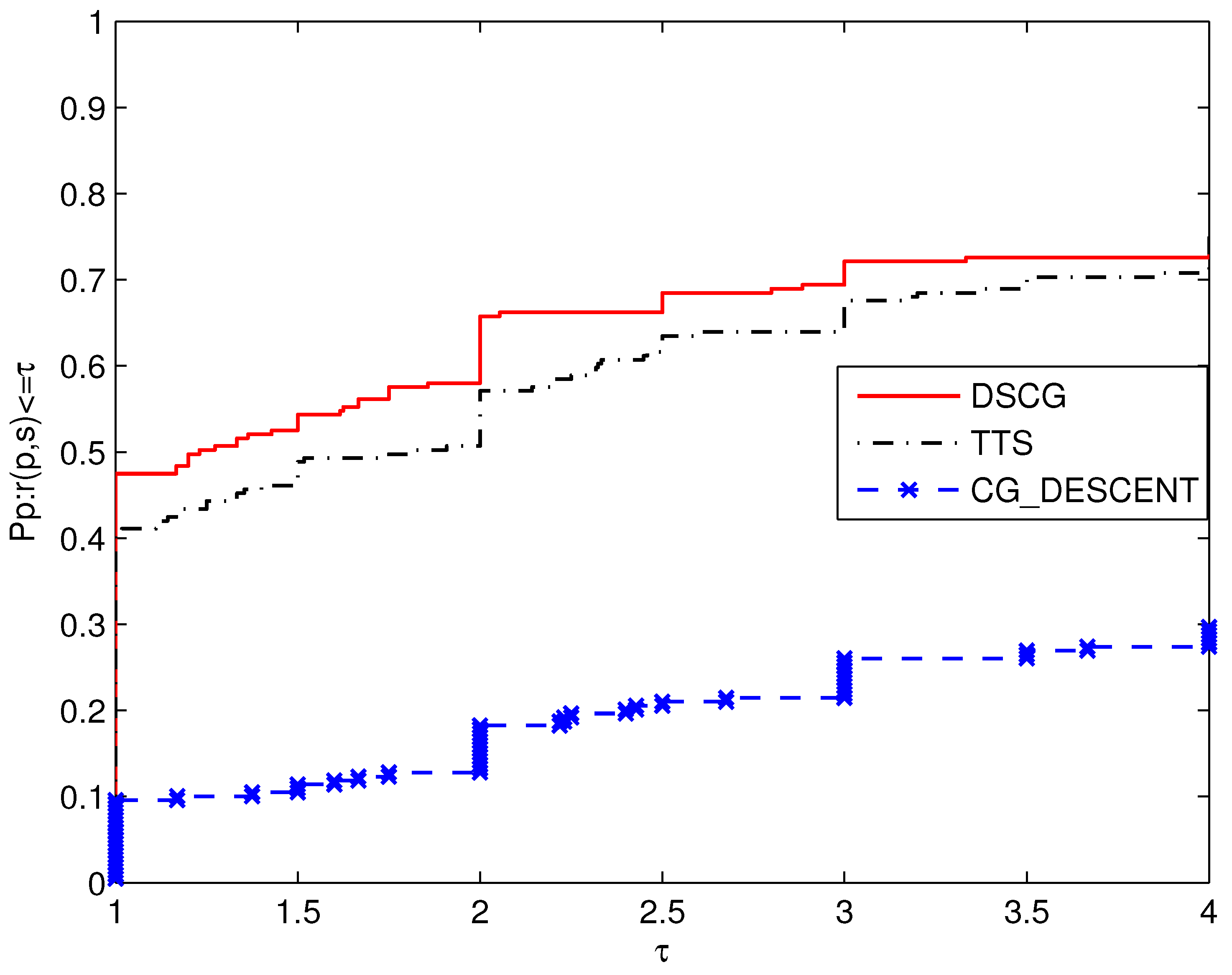
TTS and CG_DESCENT use the parameters in their code. We apply the profiles of Dolan and Moré [28] to evaluate the effectiveness of the three algorithms and discuss the performance profiles of the algorithm in CPU, NFG, and NI in detail.

The meanings of some symbols in the text are as follows:

N0: The serial number of the test problem;

CPU: The running time of algorithm (seconds);

NFG: Total evaluation numbers of function and gradient;

NI: The number of iterations.

When the problem dimension is 9000, the CG_DESCENT method only solves 64 problems, while the other two methods successfully complete all the problems. Compared with other methods, the method represented by the top curve in a performance profile drawing can solve the most problems in the best time range.

As shown in Figure 1, it is clear that the DSCG method is superior to other algorithms in terms of CPU time. Thiss corresponds to the top curve and can solve 47.49% of the test problems in the shortest time. In contrast, TTS is the fastest at solving 40.64% of the test problems, and CG_DESCENT is the fastest for only 9.59% of problems.

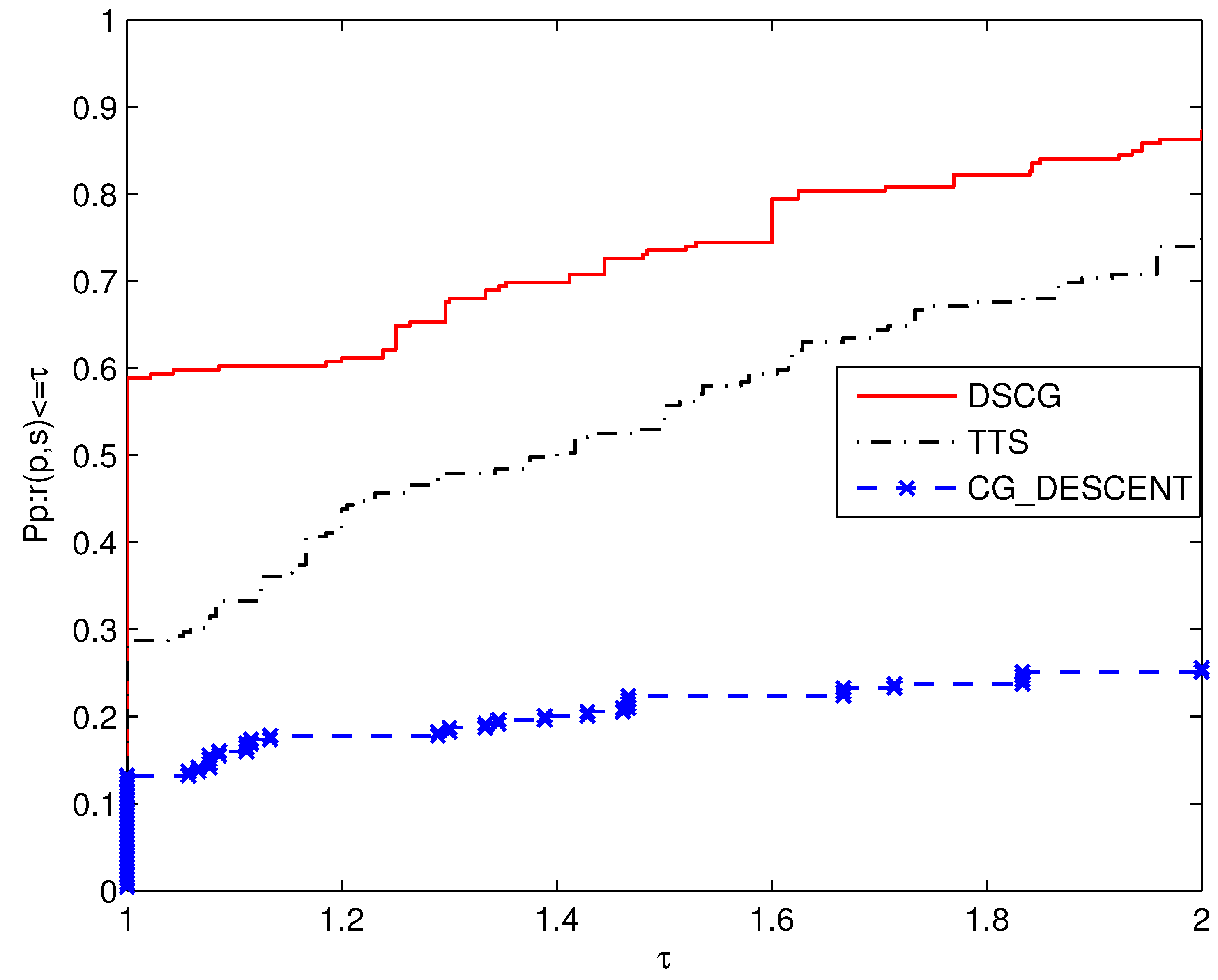
Now, let us focus on Figure 2. By comparison, it is found that DSCG requires fewer functions and gradient evaluations than other algorithms, which helps to simplify calculation and improve algorithm efficiency. It can solve 58.9% of the test problems with minimal function and gradient evaluations. TTS can solve 28.77% of the test problems with the least amount of function and gradient evaluations. The proportion of CG_DESCENT corresponds to 13.24%.

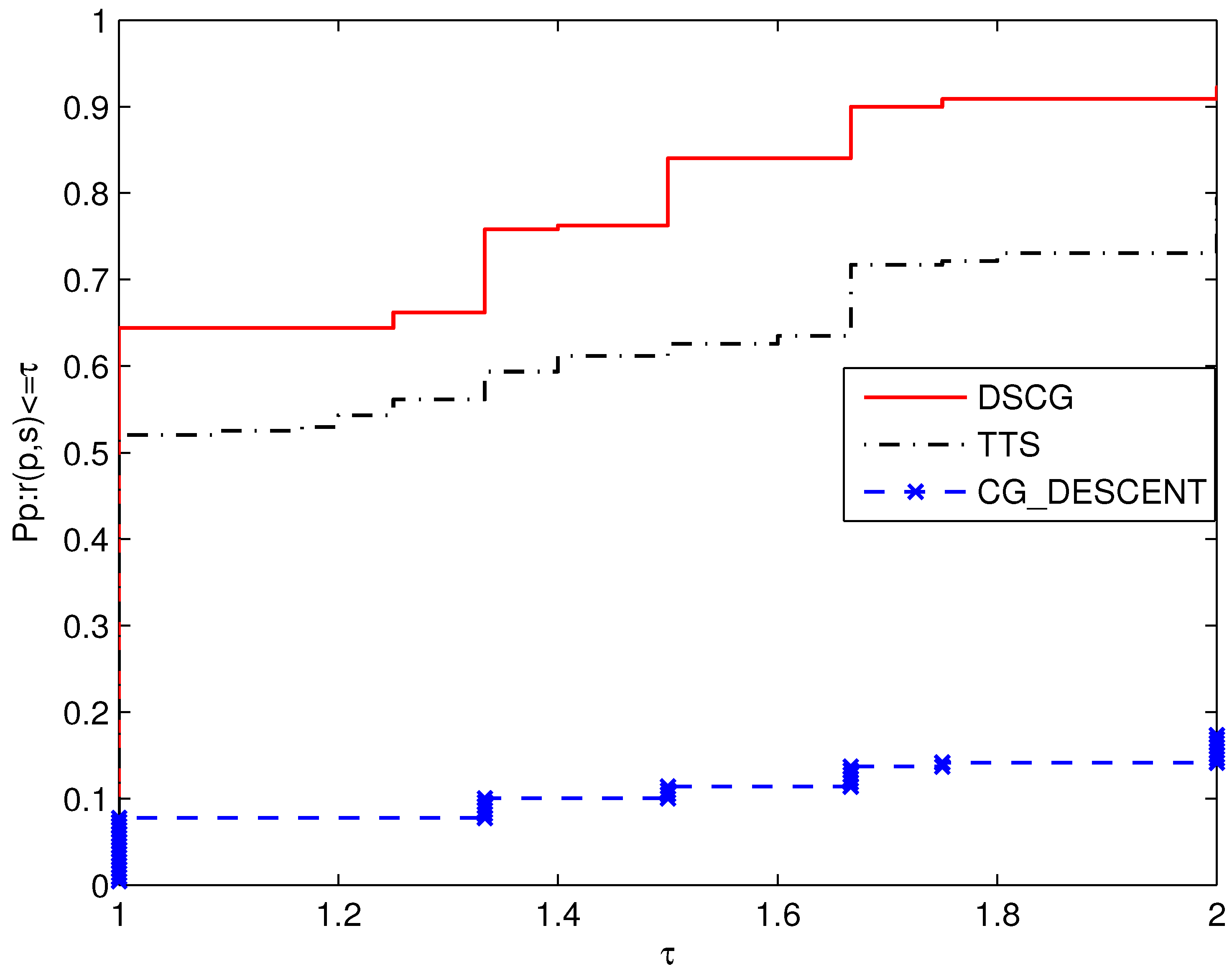
In addition, Figure 3 shows the performance comparison results of each algorithm in terms of the number of iterations. It can be seen from the figure that the performance of the DSCG algorithm is outstanding, as it can solve 64.38% of the problems with the minimum number of iterations. At the same time, TTS and CG_DESCENT have the least iterations in 52.05% and 7.76% of the problems, respectively.

The above three pictures of CPU, NFG, and NI contain some similar information. It is concluded that in the given test set, DSCG performs very well, with numerical results superior to those of TTS and CG_DESCENT.

4.2. Image Restoration Problem

The proposed DSCG is also applied to the problem of image restoration in this subsection. For more professional work in the field of image processing, please see [29,30]. In two scenes with different noise values, the blurred original image is repaired to make the picture clear and recognizable. This work has a wide range of applications in many fields of production and life, with important practical significance, and is also a difficult subject in the field of optimization. Its basic model is $b=Ax+\varsigma$, where $x\in {\Re }^n$ is the original image, $A\in {\Re }^{m\times n}$ is the blur matrix, $\varsigma \in {\Re }^m$ represents noise, and $b\in {\Re }^m$ is the image observed after noise reduction. The unknown noise value $\varsigma$ is usually obtained through

$$\underset{x\in {\Re }^n}{min}{\Vert Ax+b\Vert }^2,$$

(71)

but because the image system is susceptible to noise and lack of information, it is difficult to obtain a satisfactory solution. In order to overcome the above shortcoming, the least square model is usually introduced,

$$\underset{x\in {\Re }^n}{min}{\Vert Ax+b\Vert }^2+\lambda {\Vert \mathrm{Y}x\Vert }_1,$$

(72)

where Y is the linear operator, ${\Vert ·\Vert }_1$ represents the $l_1$ norm, and $\lambda$ is the regularization parameter used to weigh the data item and the regularization term.

Stop condition:$\frac{|f_{k+1}-f_k|}{|f_k|}<{10}^{-3}$ or $\frac{\Vert x_{k+1}\Vert -\Vert x_k\Vert }{\Vert x_k\Vert }<{10}^{-3}$;

Tested picture: Barbara ($512\times 512$), Baboon ($512\times 512$).

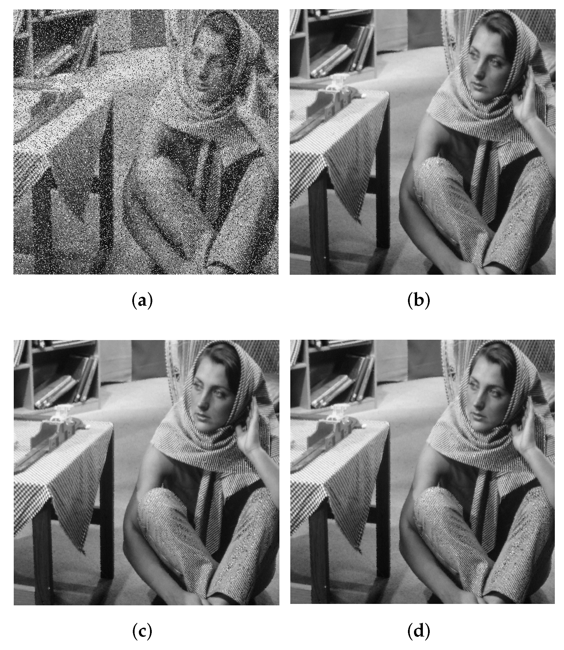
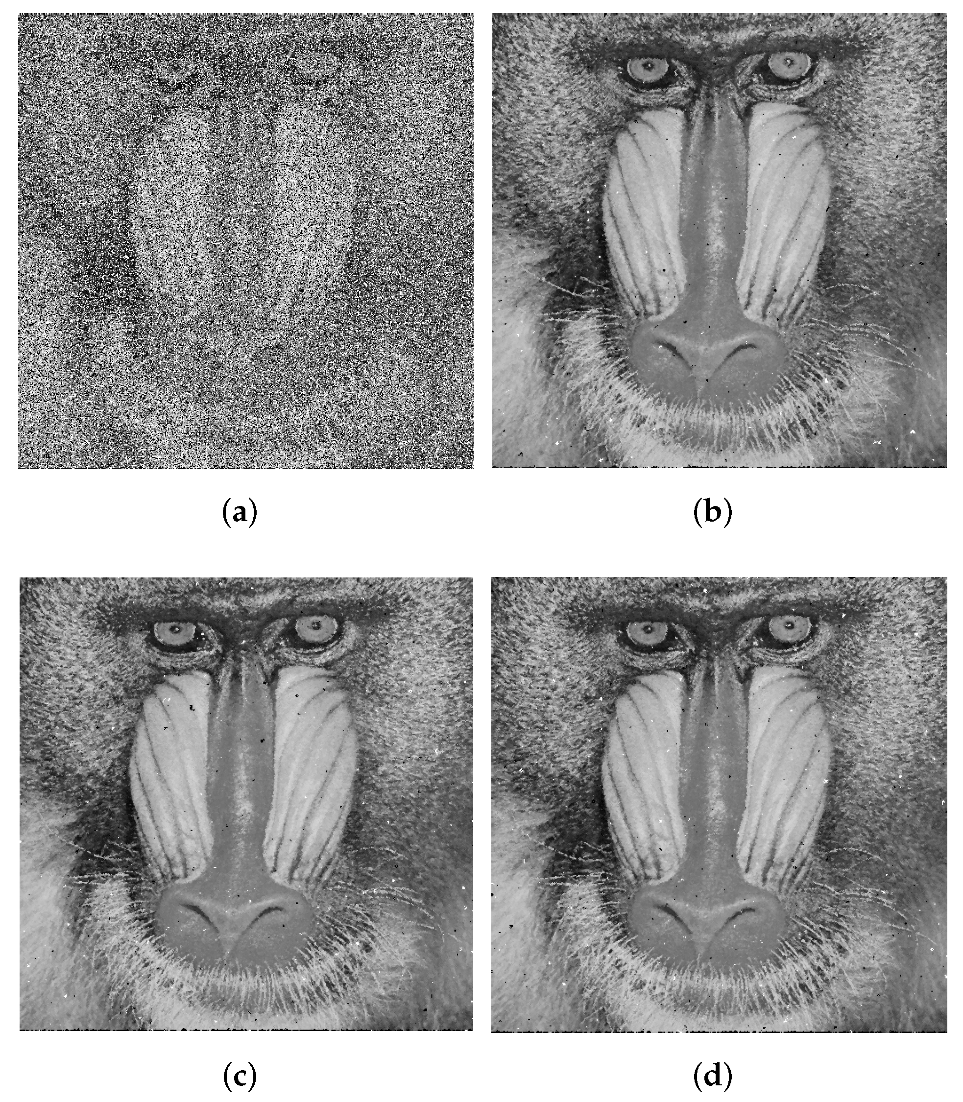
The specific image repair results of the two algorithms under different noise values are shown in Figure 4 and Figure 5. Obviously, for a given set of pictures, both algorithms successfully completed the repair. Let us focus on the comparison on

Table 2. CPU time spent by algorithms (seconds).

20% Noise	Barbara	Baboon	Total
DSCG	1.2656	1.2813	2.5469
TTS	1.2813	1.2656	2.5469
CG_DESCENT	1.4219	1.2969	2.7188
50% Noise	Barbara	Baboon	Total
DSCG	2.0625	1.9688	4.0313
TTS	2.125	2.1719	4.2969
CG_DESCENT	2.0313	2.1875	4.2188

, which presents the CPU time spent in the repair process of algorithms.

Many works have focused on the image restoration problem, and more detailed references can be found in [31,32,33,34]. In this paper, we display the original image to be repaired, and the repaired results of DSCG, TTS, and CG_DESCENT from left to right.

Summarizing the information contained in the pictures and tables in this section, we have obtained two conclusions: (i) both algorithms are capable of repairing pictures within a reasonable time frame; (ii) with noise interference of 20% and 50%, DSCG is shown to be a promising algorithm.

5. Conclusions and Discussion

In this paper, an algorithm for dynamically adjusting direction was proposed, which corresponds to the directions of four calculation forms by satisfying different conditions. We discuss the selection of directions in a special three-term subspace using modified secant equations, subspace minimization techniques, and acceleration strategies. The algorithm has a good property: each search direction satisfies the sufficient descent condition. We use the nonmonotonic generalized line search to obtain remarkable results: under some mild assumptions, we not only prove the global convergence of the general function algorithm but also further prove the R-linear convergence of the uniformly convex function. Interestingly, we apply this algorithm to image restoration, and the algorithm has good numerical performance in both the unconstrained and image restoration problems, which fully demonstrates the efficiency of this algorithm.

References

- Polyak, B.T. The conjugate gradient method in extreme problems. USSR Comput. Math. Math. Phys. 1969, 9, 94–112. [Google Scholar] [CrossRef]
- Hestenes, M.R.; Stiefel, E.L. Methods of conjugate gradient for solving linear systems. Res. Natl. Bur. Stand. 1952, 6, 409–436. [Google Scholar] [CrossRef]
- Liu, Y.L.; Storey, C.S. Efficient generalized conjugate gradient, Part I: Theory. J. Optim. Theory Appl. 1964, 7, 149–154. [Google Scholar]
- Flether, R.; Reeves, C.M. Function minimization by conjugate gradient. Comput. J. 1964, 7, 149–154. [Google Scholar] [CrossRef] [Green Version]
- Dai, Y.H.; Yuan, Y.X. A nonlinear conjugate gradient method with a strong global convergence property. SIAM J. Optim. 2000, 10, 177–182. [Google Scholar] [CrossRef] [Green Version]
- Flecther, R. Practical Methods of Optimization, Unconstrained Optimization; Wiley: New York, NY, USA, 1988; Volume I. [Google Scholar]
- Li, Y.F.; Liu, Z.X.; Liu, H.W. A subspace minimization conjugate gradient method based on conic model for unconstrained optimization. Comput. Appl. Math. 2019, 38, 16. [Google Scholar] [CrossRef]
- Dai, Y.H.; Kou, C.X. A nonlinear conjugate gradient algorithm with an optimal property and an improved Wolfe line search. SIAM J. Optim. 2013, 23, 296–320. [Google Scholar] [CrossRef] [Green Version]
- Wang, T.; Liu, Z.X.; Liu, H.W.; Wang, T.; Liu, Z.; Liu, H. A new subspace minimization conjugate gradient method based on tensor model for unconstrained optimization. Int. J. Comput. Math. 2019, 96, 1924–1942. [Google Scholar] [CrossRef]
- Li, M.; Liu, H.W.; Liu, Z.X. A new subspace minimization conjugate gradient method with nonmonotone line search for unconstrained optimization. Numer. Algorithms 2018, 79, 195–219. [Google Scholar] [CrossRef]
- Liu, H.; Liu, Z. An Efficient Barzilai-Borwein Conjugate Gradient Method for Unconstrained Optimization. J. Optim. Theory Appl. 2019, 180, 879–906. [Google Scholar] [CrossRef]
- Yuan, Y.; Stoer, J. A subspace study on conjugate gradient algorithms. Zamm J. Appl. Math. Mech. Z. Angew. Math. Mech. 1995, 75, 69–77. [Google Scholar] [CrossRef]
- Andrei, N. An accelerated subspace minimization three-term conjugate gradient algorithm for unconstrained optimization. Numer. Algorithms 2014, 65, 859–874. [Google Scholar] [CrossRef]
- Yang, Y.T.; Chen, Y.T.; Lu, Y.L. A subspace conjugate gradient algorithm for large-scale unconstrained optimization. Numer. Algorithms 2017, 76, 813–828. [Google Scholar] [CrossRef]
- Dai, Y.H.; Kou, C.X. A Barzilai-Borwein conjugate gradient method. Sci. China Math. 2016, 59, 1511–1524. [Google Scholar] [CrossRef]
- Barzilai, J.; Borwein, J.M. Two-point step size gradient methods. IMA J. Numer. Anal. 1988, 8, 141–148. [Google Scholar] [CrossRef]
- Wang, Z.H.; Yuan, Y. A subspace implementation of quasi-Newton trust region methods for unconstrained optimization. Numer. Math. 2006, 104, 241–269. [Google Scholar] [CrossRef]
- Yuan, Y.X. A review on subspace methods for nonlinear optimization. In Proceedings of the International Congress of Mathematics, Seoul, Korea, 13–21 August 2014; pp. 807–827. [Google Scholar]
- Fialko, S.; Karpilovskyi, V. Block subspace projection preconditioned conjugate gradient method in modal structural analysis. Comput. Math. Appl. 2020, 79, 3410–3428. [Google Scholar] [CrossRef]
- Hanzely, F.; Doikov, N.; Nesterov, Y.; Richtarik, P. Stochastic subspace cubic Newton method. In Proceedings of the International Conference on Machine Learning, PMLR, Montreal, QC, Canada, 6–8 July 2020; pp. 4027–4038. [Google Scholar]
- Moufawad, S.M. s-Step Enlarged Krylov Subspace Conjugate Gradient Methods. SIAM J. Sci. Comput. 2020, 42, A187–A219. [Google Scholar] [CrossRef]
- Soodhalter, K.M.; de Sturler, E.; Kilmer, M.E. A survey of subspace recycling iterative methods. GAMM-Mitteilungen 2020, 43, e202000016. [Google Scholar] [CrossRef]
- Babaie-Kafaki, S. Two modified scaled nonlinear conjugate gradient method. J. Comput. Appl. Math. 2014, 261, 172–182. [Google Scholar] [CrossRef]
- Yao, S.; Wu, Y.; Yang, J.; Xu, J. A three-term gradient descent method with subspace techniques. Math. Probl. Eng. 2021, 2021, 8867309. [Google Scholar] [CrossRef]
- Andrei, N. An acceleration of gradient descent algorithm with backtracking for unconstrained optimization. Numer. Algorithms 2006, 42, 63–73. [Google Scholar] [CrossRef]
- Zhang, H.C.; Hager, W.W. A nonmonotone line search technique and its application to unconstrained optimization. SIAM J. Optim. 2004, 14, 1043–1105. [Google Scholar] [CrossRef] [Green Version]
- Hager, W.W.; Zhang, H. A new conjugate gradient method with guaranteed descent and an efficient line search. SIAM J. Optim. 2005, 16, 170–192. [Google Scholar] [CrossRef] [Green Version]
- Dolan, E.D.; Moré, J.J. Benchmarking optimization software with performance profiles. Math. Program. 2002, 91, 201–203. [Google Scholar] [CrossRef]
- Versaci, M.; Calcagno, S.; Morabito, F.C. Fuzzy geometrical approach based on unit hyper-cubes for image contrast enhancement. In Proceedings of the 2015 IEEE International Conference on Signal and Image Processing Applications (ICSIPA), Kuala Lumpur, Malaysia, 19–21 October 2015; pp. 488–493. [Google Scholar]
- Rahim, S.S.; Palade, V.; Shuttleworth, J.; Jayne, C. Automatic screening and classification of diabetic retinopathy and maculopathy using fuzzy image processing. Brain Inform. 2016, 3, 249–267. [Google Scholar] [CrossRef] [PubMed]
- Hanjing, A.; Suantai, S. A fast image restoration algorithm based on a fixed point and optimization method. Mathematics 2020, 8, 378. [Google Scholar] [CrossRef] [Green Version]
- Padcharoen, A.; Kitkuan, D. Iterative methods for optimization problems and image restoration. Carpathian J. Math. 2021, 37, 497–512. [Google Scholar] [CrossRef]
- Ibrahim, A.H.; Kumam, P.; Kumam, W. A family of derivative-free conjugate gradient methods for constrained nonlinear equations and image restoration. IEEE Access 2020, 8, 162714–162729. [Google Scholar] [CrossRef]
- Fessler, J.A. Optimization methods for magnetic resonance image reconstruction: Key models and optimization algorithms. IEEE Signal Process. Mag. 2020, 37, 33–40. [Google Scholar] [CrossRef]
Figure 1.
Performance profiles for the CPU.
Figure 2.
Performance profiles for the NFG.
Figure 3.
Performance profiles for the NI.
Figure 4.
20% noise. (a) original image; (b) DSCG; (c) TTS; (d) CG_DESCENT.
Figure 5.
50% noise. (a) original image; (b) DSCG; (c) TTS; (d) CG_DESCENT.