
Multinomial Logit Model Building via TreeNet and Association Rules Analysis: An Application via a Thyroid Dataset

Department of Mathematics, Faculty of Science, Mahidol University, Bangkok 10400, Thailand
Symmetry 2021, 13(2), 287; https://doi.org/10.3390/sym13020287
Submission received: 15 January 2021
/
Revised: 1 February 2021
/
Accepted: 4 February 2021
/
Published: 8 February 2021
(This article belongs to the Special Issue Modelling and Simulation of Natural Phenomena of Current Interest)
Abstract
:A model-building framework is proposed that combines two data mining techniques, TreeNet and association rules analysis (ASA) with multinomial logit model building. TreeNet provides plots that play a key role in transforming quantitative variables into better forms for the model fit, whereas ASA is important in finding interactions (low- and high-order) among variables. With the implementation of TreeNet and ASA, new variables and interactions are generated, which serve as candidate predictors in building an optimal multinomial logit model. A real-life example in the context of health care is used to illustrate the major role of these newly generated variables and interactions in advancing multinomial logit modeling to a new level of performance. This method has an explanatory and predictive ability that cannot be achieved using existing methods.
1. Introduction
The multinomial logit model is the fundamental method used to predict and explain a multi-category response. In related studies, researchers have developed a number of ways to select and screen variables with the goal of advancing the multinomial logit model. These include the likelihood-based boosting technique used with one step of Fisher scoring to select the variables [1] and a five-step technique drawing on analysis of variance (ANOVA) and bootstrapping aggregation used to screen the variables [2]. However, neither of these approaches accounts for the interactions between variables in the selection process. Camminatiello and Lucadamo [3] advanced the model by applying principal component analysis (PCA) and thereby removing the problem of multicollinearity data. Kim and Kim [4] also focused on interactions in developing a two-stage methodology that relies on combining a decision tree with the multinomial logit model: the decision tree provides the basis for selecting influential interaction effects that serve as the explanatory variables for fitting the multinomial logit model. However, the decision tree has the drawback of a hierarchical structure.
In our previous work, Changpetch and Lin [5], we used ASA, specifically classification rule mining (CRM), to search for potential rules, which are then converted into potential interactions (low- and high-order) to serve as candidate predictors for the multinomial logit model. We used ASA, because unlike the decision tree it allows for a global search through which more potential interactions can be located and thus considered. In that procedure, however, the use of quantitative predictors is limited, as ASA can generate rules for categorical predictors only.
In this paper, we develop a model-building framework that improves on other approaches to multinomial logit model building by combining methods for variable discretization, variable transformation, interaction generation, and variable selection in one framework. In conjunction with the multinomial logit model, two data mining techniques are used in this framework: TreeNet, for variable discretization and variable transformation, and ASA, for generating and selecting the interactions.
A data mining technique built on classification and a decision tree [6], TreeNet has the special feature of providing dependency plots that can be used to help discretize quantitative predictors into categories and then transform the predictors into various forms that have the potential to improve the model fit. These newly generated variables are then used to find the interactions and also to serve as candidate predictors for the optimal multinomial logit model. Note that the present study constitutes the first account in which TreeNet is used as the discretization method.
We use ASA to find relationships between the response and the categorical variables in terms of rules. However, ASA works only with categorical variables, which means that quantitative predictors have limited use in this method [5,6]. It is possible, though, to overcome this limitation. The inclusion of TreeNet in the proposed model means that the new categorical variables, which are generated by discretizing the original quantitative predictors, work with ASA, such that the limitation does not apply in this context.
With the combined use of TreeNet and ASA, new variables and interactions, both low- and high-order, are generated. These new generated variables and interactions, combined with the original variables, are all considered in determining the optimal multinomial logit model, which is the last step in the framework proposed herein. We illustrate the proposed model-building framework through a thyroid dataset, and on this basis, we prove that our method significantly outperforms the existing options by improving the model fit. On this basis, we demonstrate that multinomial logit modeling achieves a new level of performance in terms of predictive accuracy.
2. Generating Variables and Interactions with TreeNet and Association Rules Analysis for the Multinomial Logit Model
The multinomial logit model is a fundamental statistical model used to explore relationships between and among variables and to predict the classes of multiple-level responses. In this study, we focus on the multi-category response without orders or nominal data. For this type of response, we use the baseline-category logit model, which combines the separate binary logit model for each pair of response categories [7,8]. Response (Y) has J categories, and J, the last level, is the base level. Therefore, let denote the probability in class j for response Y at a fixed setting of x and let the summation for all categories of the response equal 1, i.e., . Thus, the logit model pairs each response with a baseline category, which is often the last or the most common category. The following model describes the effects of x on these J − 1 logits:
where is an intercept and are coefficients of the predictors x.
The multinomial logit model is based on the assumption of a linear relationship between the logit (left-hand side of the equation) and each of the quantitative variables (right-hand side of the equation). However, it is usual for some of the quantitative variables to have a non-linear relationship with the logit across the entire range of their values. That is, any given quantitative variable may include a combination of linear functions and step functions. Accordingly, partitioning the variable into categories with the appropriate function for each category should be helpful in fitting the model. With this in mind, we have found TreeNet to be a very effective method for partitioning and transforming variables, as we will demonstrate.
2.1. TreeNet
A data mining method developed from the classification tree and the regression tree (CART), TreeNet can be used with either a quantitative or a categorical response [6]. TreeNet begins with a small tree, and then a second tree is grown to predict the residuals from the first tree. Next, a third tree is grown to predict the residuals from the combination of the first two trees. Additional trees are then grown to predict the residuals from the combination of the previous trees. This process is repeated until a given number of trees have been developed.
A TreeNet model can consist of hundreds or thousands of trees. However, the summary of TreeNet is shown directly via two plots—the variable importance plot and the partial dependency plot—both of which greatly facilitate the procedure we propose. The variable importance plot provides the score that each variable contributes to predicting the response. This is the relative importance score, which rescales the raw variable importance score so that the most important variable always receives a score of 100 [6]. The raw variable importance score is computed as the cumulative sum of the improvements of all the splits associated with a given variable across all trees up to a specific model size. This plot is useful for analysis because it shows which variables have scores above zero, i.e., the variables we need to focus on in the model.
The partial dependency plot shows the relationship between each variable, and the logit after the effects of the other variables is accounted for. This plot is constructed by fixing the values of the other variables at the joint set while finding the dependency curve of the variable of interest over its range with the logit. The process is then repeated with different joint sets of values for each of the other variables in order to find the other curves. The values of all these curves are averaged and centered to obtain the partial dependency plot for the given variable of interest [6]. Note that a partial dependency plot will be created only for variables with scores higher than zero. With these dependency plots, we can partition each quantitative variable into categories based on the respective function of the relationship of each variable with the logit. For this study, we applied TreeNet models (https://www.minitab.com/en-us/products/spm/tree-net/, accessed on 18 February 2020).
A number of discretization methods are used in data mining [9], including (i) equal width discretization (EWD) [10,11], which divides the range of the quantitative variable into intervals with equal width for each interval; (ii) equal frequency discretization (EFD) [10,11], which divides the range of the quantitative variable into intervals with an equal or approximately equal number of observations; (iii) fuzzy discretization (FD) [12,13], which is based on the idea that the impact of the value to the probabilities depends on its variation; (iv) entropy minimization discretization (EMD) [14], which uses entropy as the criterion to find the splitting values; (v) iterative discretization (ID) [15], which forms a set of intervals using a basic discretization method such as EWD and then adjusts the intervals to maximize classification accuracy; (vi) proportional k-interval discretization (PKID) [16], which is developed from the idea that discretization bias and variance depend on interval size and interval number; (vii) lazy discretization (LD) [9,17], which determines the splitting value when the test instance is presented; (viii) non-disjoint discretization (NDD) [18], which is based on the idea that intervals with quantitative variable values closer to the midpoint will give better probability estimation than will intervals with quantitative variable values closer to the boundary; (ix) weighted proportional k-interval discretization (WPKID) [19], which is similar to PHID but assigns more weight to discretization variance reduction than to bias reduction.
However, we selected TreeNet as the discretization method because it is the only technique that provides the function of each interval of the predictors in relation to the logit via the partial dependency plot. Using this plot, we can attach the function, e.g., the linear function, appropriately to each interval.
2.2. Association Rules Analysis (ASA)
In model building, accounting for interactions is always important in improving the quality of a model. Yet, in the multiple logit model, interactions have been put to only limited use in building models. In particular, interactions between categorical variables are typically excluded from classical multinomial logit models [5,8,20]. However, in the present study, we find that interaction effects are the key to improving the model fit for the multinomial logit model. Furthermore, using ASA, we find an effective way to identify potential interactions (both low- and high-order) for this kind of model.
ASA is a well-known methodology used to analyze the relationships among items in terms of rules. Similarly, it can be applied to find relationships among variables, and CRM, a specific kind of ASA technique, can be used for classification purposes. For example, assume that we have k binary predictors, X1, X2, X3, …, Xk, and a binary response, Y. Each variable has two levels denoted by 0 and 1. Many rules can be generated. As an example, the first rule could be “If X1 = 1, X2 = 0, then Y = 1” and the second rule could be “If X1 = 0, X2 = 1, X3 = 1, then Y = 1”.
From the many rules generated, two measurements are used to select a set of rules to serve as a classifier for the dataset. These two measurements are support (s) and confidence (c) [5,7,21]. Support (s) is the probability of the left-hand side item(s) and the right-hand side item. From the given example, support (s) for the first rule is equal to P (X1 = 1, X2 = 0 and Y = 1), and support (s) for the second rule is equal to P (X1 = 0, X2 = 1, X3 = 1 and Y = 1). The second measurement is confidence (c), which is the probability of the left-hand side item(s) and the right-hand side item(s) divided by the probability of the left-hand side item(s). From the example, confidence (c) for the first rule is equal to P (X1 = 1, X2 = 0, and Y = 1)/P (X1 = 1 and X2 = 0) and confidence (c) for the second rule is equal to P (X1 = 0, X2 = 1, X3 = 1, and Y = 1)/P (X1 = 0, X2 = 1, X3 = 1). Similar to ASA, CRM finds all the rules that meet two key thresholds: minimum support and minimum confidence [22]. These selected rules will be used to form a classifier [23,24].
3. Proposed Method
The proposed framework for building a multinomial logit model consists of five key steps:
Step 1: Utilize TreeNet to discretize each quantitative explanatory variable into categories and transform these categories into new variables.
Step 2: Utilize CRM, a subset of ASA, to generate rules from all the categorical variables, i.e., the new categorical variables generated in step 1 and the original categorical variables.
Step 3: Select the rules based on the rules selection criterion.
Step 4: Generate the interactions for each rule selected in step 3.
Step 5: Search for the optimal multinomial logit model based on the variables generated in step 1, the interactions generated in step 4, and the original variables.
- Step 1:
- Discretization
In step 1, we discretize the quantitative variables into categories using TreeNet for two purposes: (i) to create new variables with the potential to provide a better fit than the original variables do and (ii) to use the new variables to develop interactions using CRM, as this method works only with categorical variables. TreeNet is used to provide partial dependency plots, which we then use to assign the quantitative variables to categories.
For a response with J classes, referred to as 1, 2, …, J, where J is the base class, we fit J − 1 TreeNet classification models. We fit each model for the response with only two classes: class j, where j = 1, 2, J − 1, and class J, which is the base class. Therefore, we extract the data from each of the two classes from the original dataset to fit each model. After fitting each model, we observe the dependency plot of each quantitative variable. For each plot, we take the original variables and categorize their parts according to their respective functions with the logit. Next, we convert these categories into binary variables. If a part of a quantitative variable has a linear relationship with the logit, an additional variable is generated by attaching the linear function to that part. We provide an example via an application in the next section.
- Step 2:
- Rules Generation
In step 2, we use CRM to create rules from datasets. The candidate variables for generating the rules are (i) all the original categorical variables and (ii) all the newly generated binary variables from step 1. In this step, we use the CBA program developed by the Department of Information Systems and Computer Sciences at the National University of Singapore [23] to perform CRM. We generally set the minimum support to 10% and the minimum confidence to 80% [7]. However, the values can be modified based on the characteristics of the dataset, as we will demonstrate via the application in the next section. All the rules with support (s) and confidence (c) that satisfy the minimum support and minimum confidence are referred to as active rules and constitute the input for step 3. Note that all the rules are in the form of “If Xi’s = xi’s, then Y = y,” where xi is the level of predictor Xi and y the level of response Y.
- Step 3:
- Rules Selection
In step 3, we select the rules to convert into interaction variables for use in step 4. In our previous work [5,7,25], we recommend selecting the rules with the highest confidence from among all the rules obtained in step 2. Between 30 and 50 rules are selected. The number of rules can be higher for a dataset with a very high number of predictors. However, our empirical studies show that rules selected as classifier rules via CBA [23] can be used. Note that classifier rules are selected rules that form a classifier for the dataset. Furthermore, these rules from CBA yield a result that is comparable to the result for the rule selection criterion we recommend selecting. The number of classifier rules is always less than 50; therefore, we can simplify the rule-selection process by selecting all the classifier rules. Note that classifier rules can always be found even when software other than CBA is used. We refer to the rules selected at this stage as potential rules.
- Step 4:
- Variable Generation
In this step, the interactions are generated from the potential rules in step 3. Assume that one of the potential rules is in this form: “If Xi = xi, Xj = xj, and Xk = xk, then Y = y”. The interaction between the predictors Xi, Xj, and Xk from this rule is generated by setting this interaction as 1 if Xi = xi, Xj = xj, and Xk = xk, and as 0 otherwise. This interaction is denoted by Xi(xi)Xj(xj)Xk(xk). For example, for the rule “If X1 = 1, X2 = 1, and X3 = 1, then Y = 1”, we create an interaction between X1, X2, and X3 denoted by X1(1)X2(1)X3(1). In this case, X1(1)X2(1)X3(1) = 1, if X1 = 1, X2 = 1, and X3 = 1, and 0 otherwise. Note that the level of Y in each rule does not have any role in generating the interactions.
- Step 5:
- Model Selection
In step 5, any model selection criterion and any model-building method can be used. Here, the stepwise regression and Bayesian information criterion (BIC) are used for the purpose of illustration [26].
4. Illustrated Example: Thyroid Dataset
We will use the thyroid dataset retrieved from UCI machine learning (https://archive.ics.uci.edu/ml/datasets/Thyroid+Disease, accessed on 28 May 2020) to demonstrate our method. We selected this dataset because it is large and practical [27] and because of these qualities it has been used to demonstrate numerous classification methods [27,28,29]. The dataset provides information on the thyroid function of 3488 patients: 3204 (92.47%) with normal function, 93 (2.47%) with hypo-function, and 191 (5.06%) with hyper-function [30]. There are 21 predictors in the dataset. The objective of this analysis is to classify the patients as normal (class 0), hypo-function (class 1), or hyper-function (class 2), and to explain the relationships between the predictor and the probability of a patient belonging to each of the three classes. As the normal class accounts for more than 92% of the patients, for a classifier to be useful it must classify the patients into the correct class at a rate significantly above this percentage [27]. The 21 predictors are listed together with some descriptive details in Table 1.
For this dataset, there are 15 categorical predictors (X2–X16) and six quantitative predictors (X1, X17–X21).
Step 1: Discretize the quantitative variables into categories using TreeNet. As there are three classes, we fit two TreeNet models. For Model 1, the response comprises two classes: class 0 (base level) and class 1. For Model 2, the response comprises two classes: class 0 (base level) and class 2. For each model, we fit the response by all 21 original variables (X1–X21). The variable importance plot of Model 1 is shown in Table 2.
4.1. Results from Model 1
From Table 2, the most important predictor contributing to predicting the response is TSH (X17), with a score of 100. The second most important predictor is FTI (X21), with a score of 63.88. We can observe that all six quantitative variables contribute to predicting the response, as each quantitative variable has a score higher than zero. The dependency plots of all the quantitative variables are shown in Figure 1, Figure 2, Figure 3, Figure 4, Figure 5 and Figure 6: the vertical axis represents a 0.5[log(p1/p0)], where p1 is the probability that the variable is in class 1 and where p0 is the probability that the variable is in class 0. For simplicity, we refer to 0.5[log(p1/p0)] as the logit or log-odds. The interpretation from TreeNet is based on comparing the relative values of the log-odds; i.e., the higher the value of the log odds, the higher the probability that a variable is in class 1.
From the partial dependency plot, we take each quantitative variable and assign each of its parts to categories according to their respective functions to the logit. After the original variables are divided into parts, new variables are generated as binary variables (Table 3). Please note that TreeNet by Salford Systems includes a feature that shows which values of the predictors constitute the separating points.
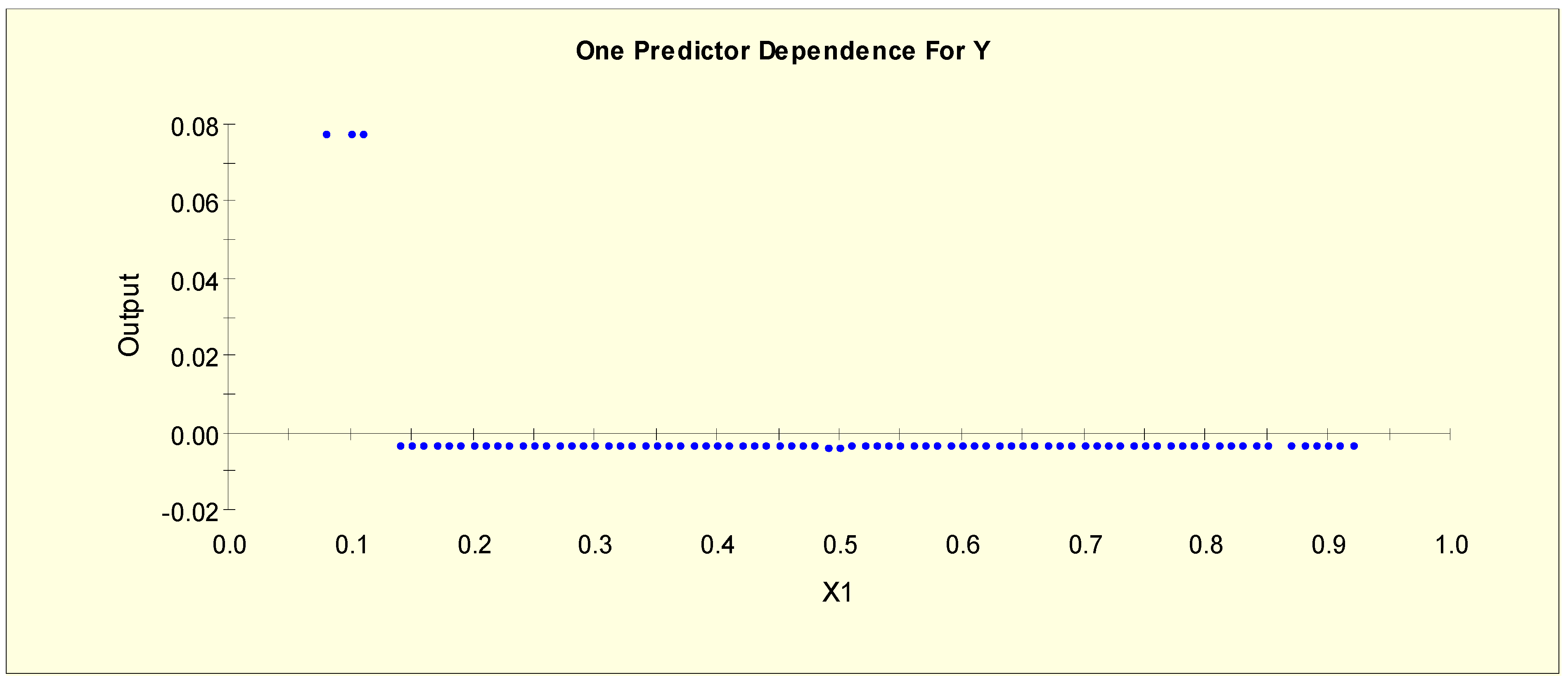
Figure 1 shows the partial dependency plot, which indicates the relationship between TSH (X17) and the log-odds from Model 1. From this plot, we can separate X17 into two levels given that the log-odds value shifts to a different level when X17 = 0.025, i.e., the splitting value is 0.025. The two binary variables, X17L1 and X17L2, are generated as shown in Table 3.
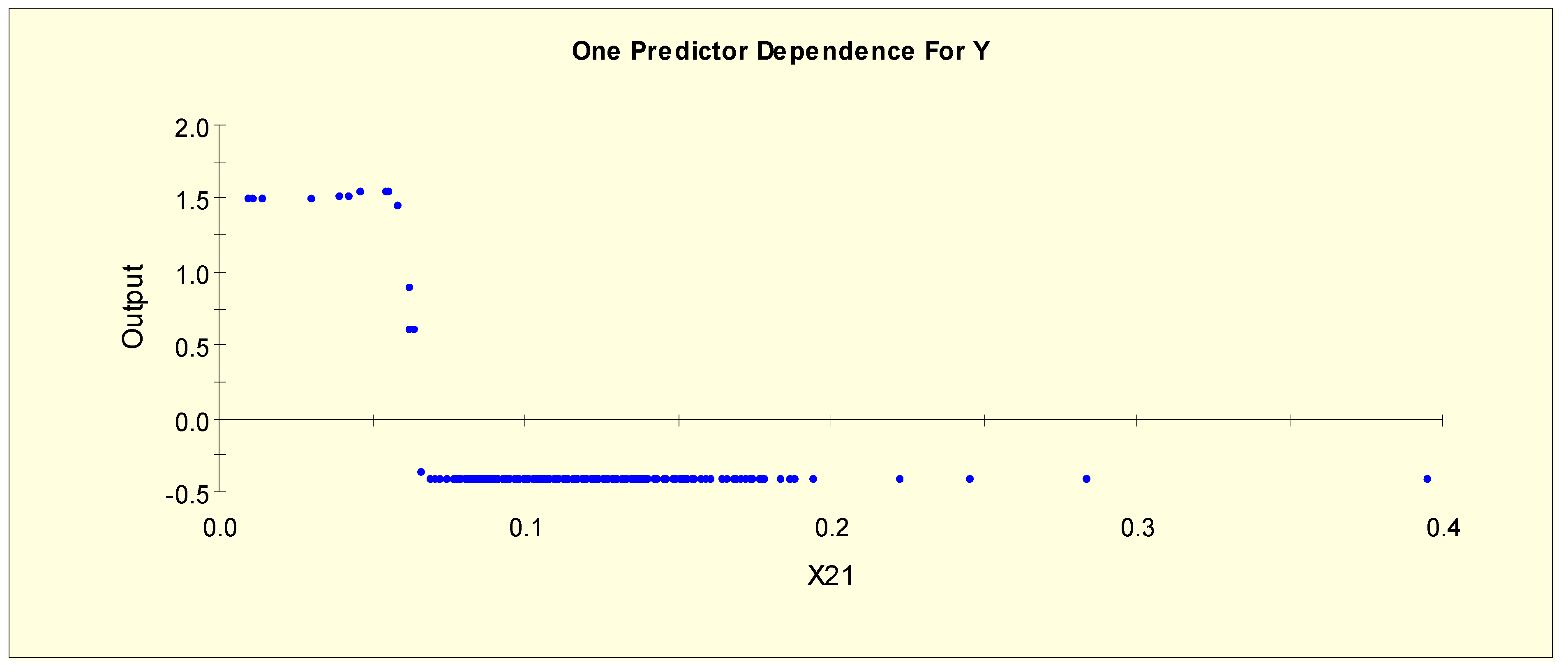
Figure 2 shows the partial dependency plot, which indicates the relationship between FTI (X21) and the log-odds from Model 1. From this plot, we can separate X21 into three levels given that the log-odds value stays constant and then shows a downward slope when X21 = 0.055. The downward slope stops when X21 = 0.07, and there is no change in the log-odds after this value. Therefore, this predictor is separated into three levels with two splitting values, 0.055 and 0.07. The three binary variables, X21L1, X21L2, and X21L3, are generated as shown in Table 3.
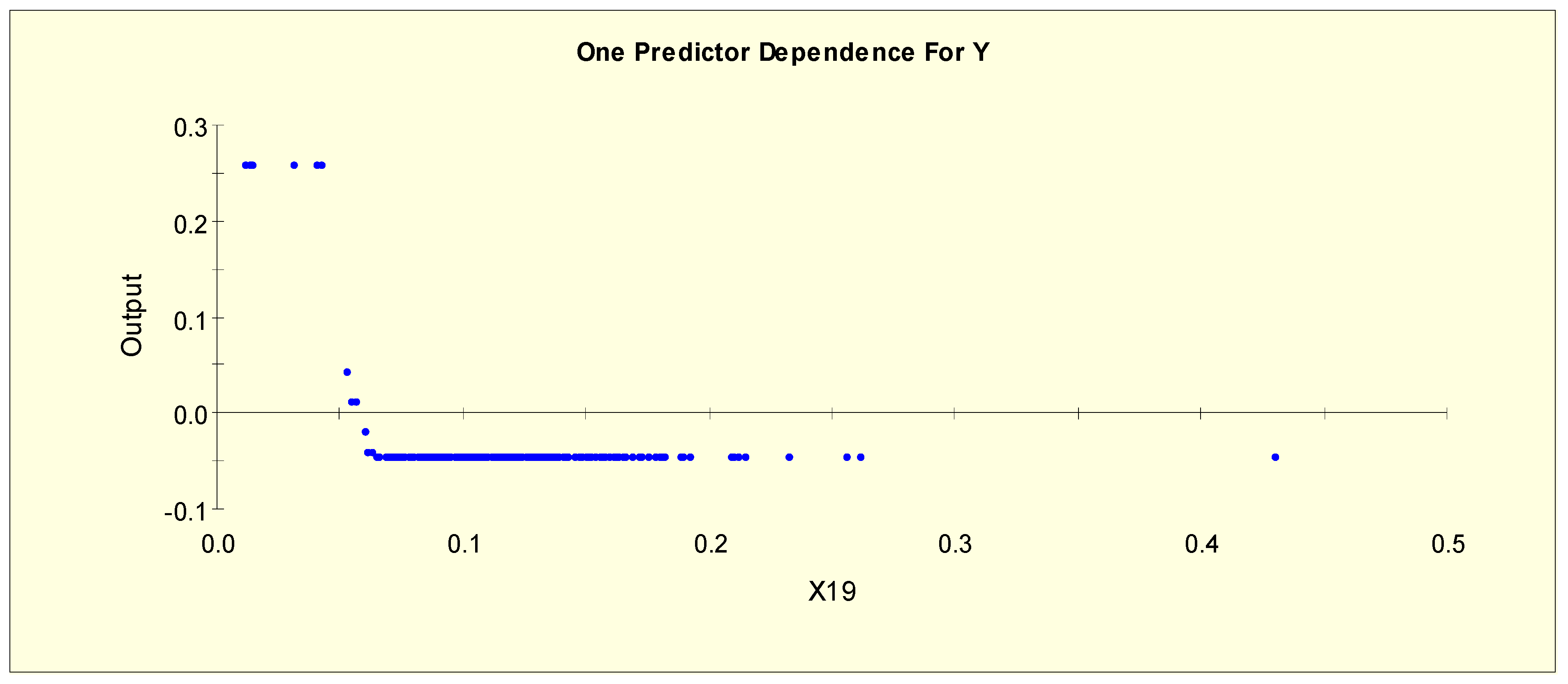
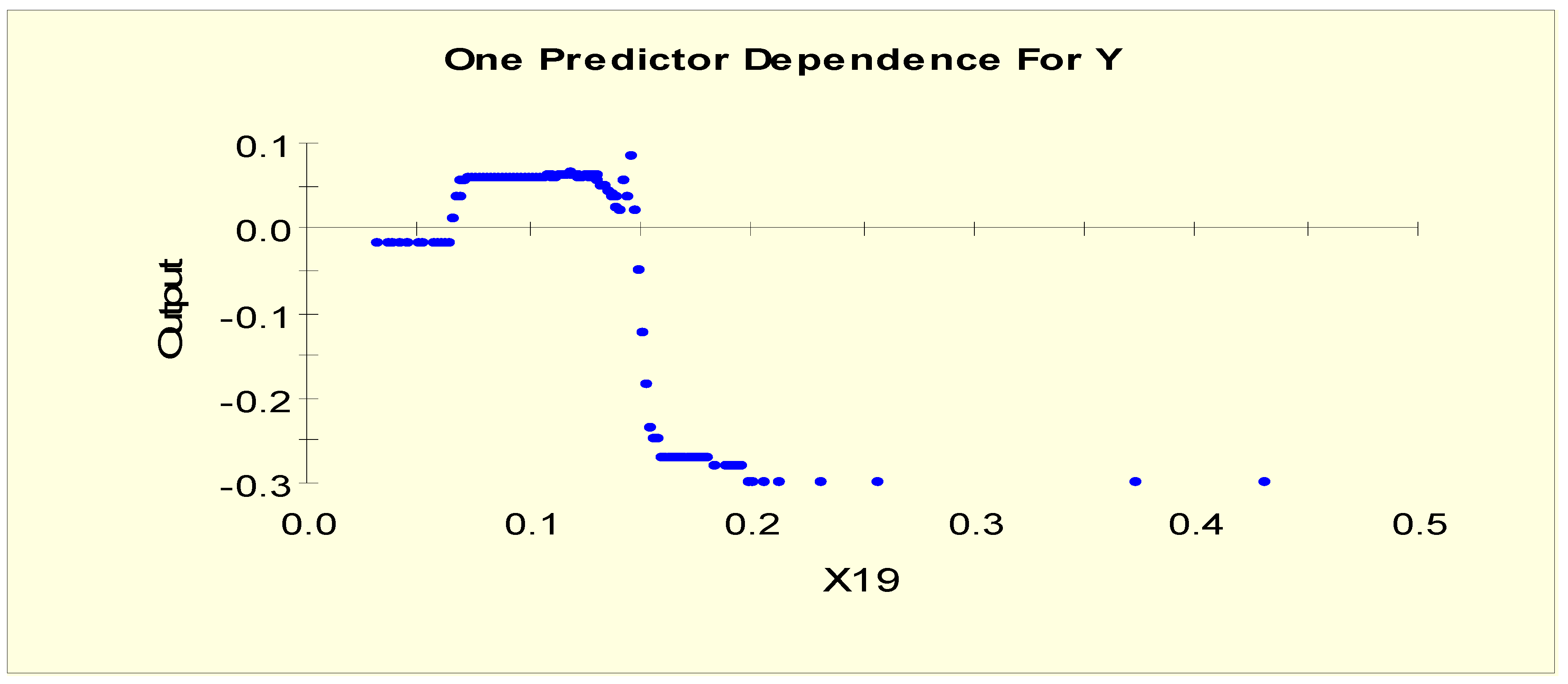
Figure 3 shows the partial dependency plot, which indicates the relationship between TT4 (X19) and the log-odds from Model 1. From this plot, we can separate X19 into three levels given that the log-odds value stays constant and then shows a downward slope when X19 = 0.042. The downward slope stops when X19 = 0.065, and there is no change in the log-odds after this value. Therefore, this predictor is separated into three levels with two splitting values, 0.042 and 0.065. The three binary variables, X19L1, X19L2, and X19L3, are generated as shown in Table 3.
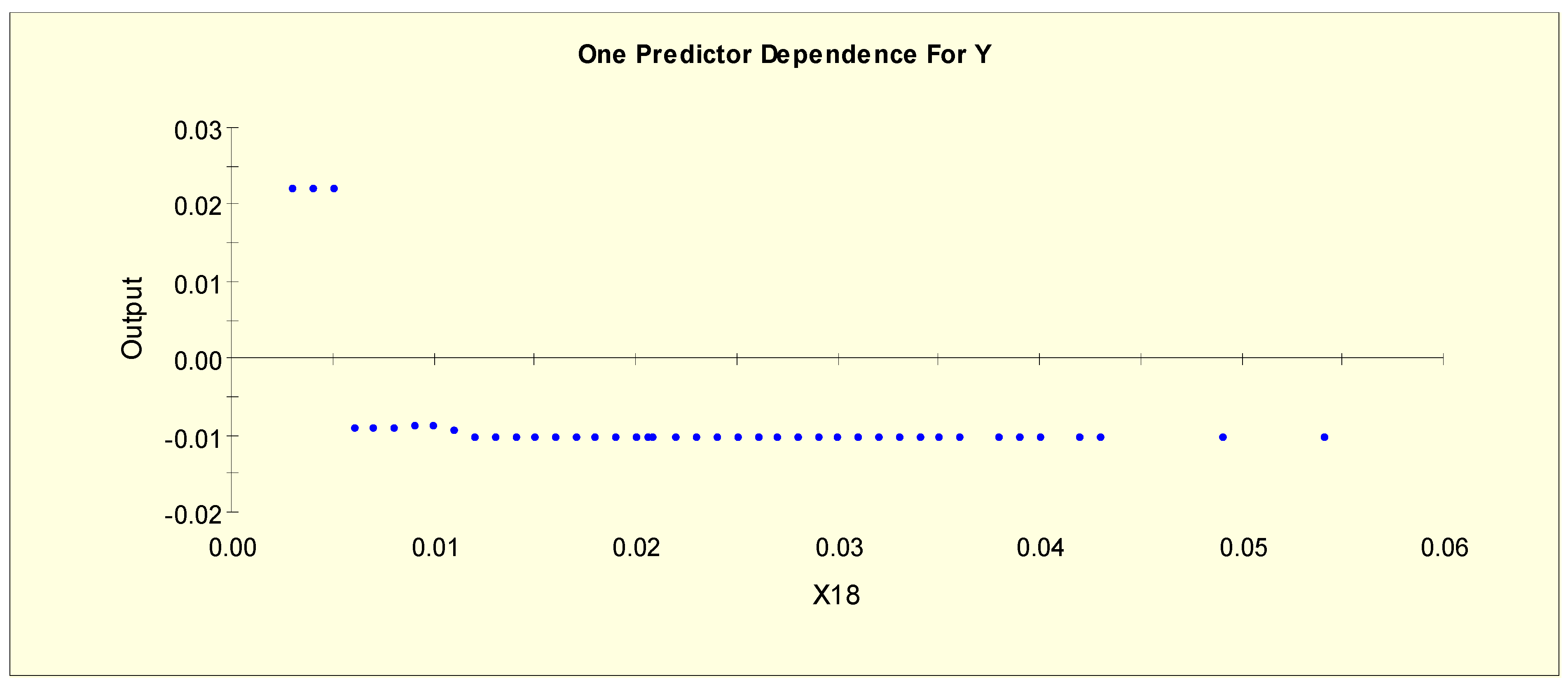
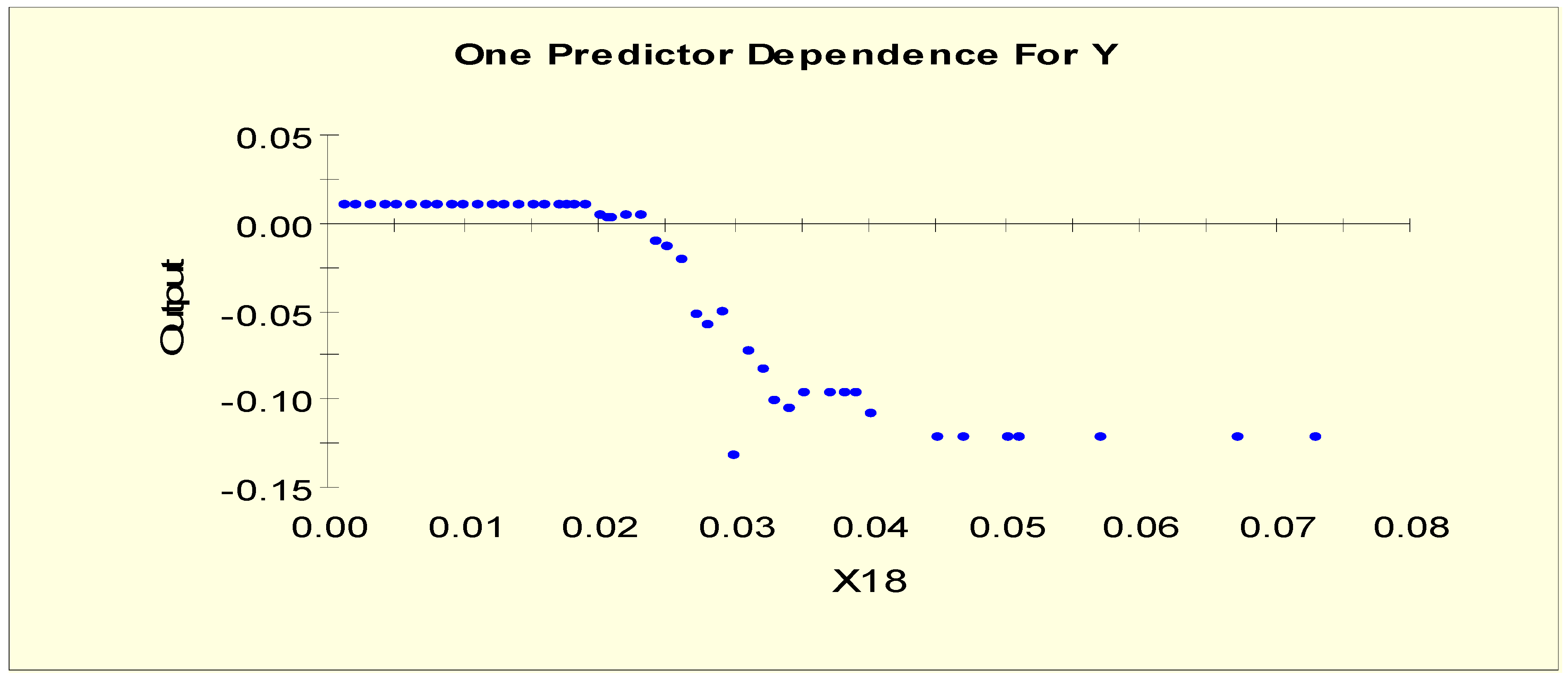
Figure 4 shows the partial dependency plot, which indicates the relationship between T3 (X18) and the log-odds from Model 1. From this plot, we can separate X18 into two levels given that the log-odds value drops to a different level when X18 = 0.006, i.e., the splitting value is 0.006. The two binary variables, X18L1 and X18L2, are generated as shown in Table 3.
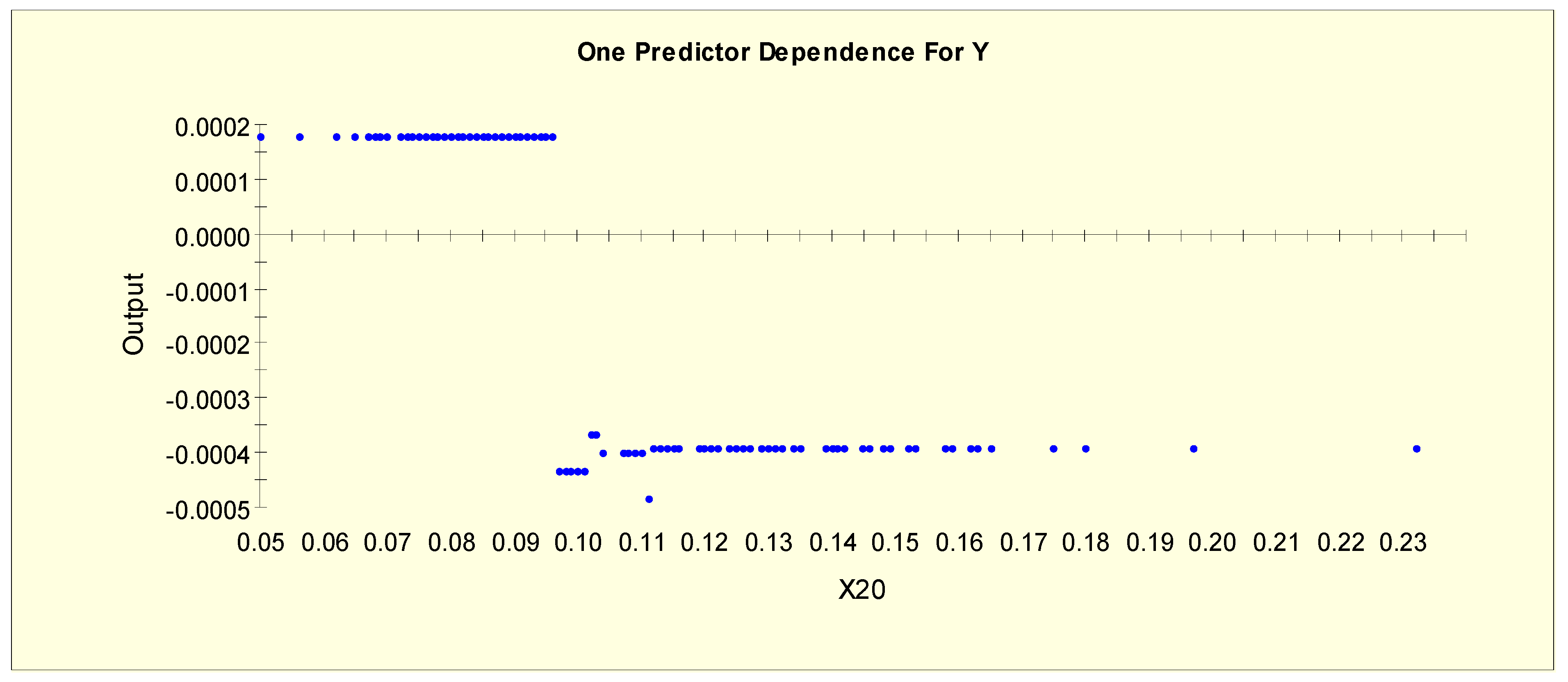
Figure 5 shows the partial dependency plot, which indicates the relationship between T4U (X20) and the log-odds from Model 1. From this plot, we can separate X20 into two levels given that the log-odds value drops to a different level when X20 = 0.097, i.e., the splitting value is 0.097. The two binary variables, X20L1 and X20L2, are generated as shown in Table 3.
Figure 6 shows the partial dependency plot, which indicates the relationship between age (X1) and the log-odds from Model 1. From this plot, we can separate X1 into two levels given that the log-odds value drops to a different level when X1 = 0.15, i.e., the splitting value is 0.15. The two binary variables, X1L1 and X1L2, are generated as shown in Table 3.
The second categories of X21 and X19 show a linear trend. Therefore, there are two more variables to generate for these two categories (Table 4).
4.2. Results from Model 2
The variable importance plot for Model 2 is shown in Table 5.
From Table 5, the most important predictor that contributes to predicting the response is TSH (X17), with a score of 100. The second most important predictor is thyroxine (X3), with a score of 44.88. We can observe that all six quantitative variables contribute to predicting the response, as each quantitative variable has a score higher than zero. The dependency plots of all the quantitative variables are shown in Figure 7, Figure 8, Figure 9, Figure 10, Figure 11 and Figure 12: the vertical axis represents a 0.5[log(p2/p0)], where p2 is the probability that a variable is in class 2 and where p0 is the probability that a variable is in class 0. The higher the value of the log-odds, the higher the probability that a variable belongs in class 2.
From Figure 7, Figure 8, Figure 9, Figure 10, Figure 11 and Figure 12, we take each quantitative variable and assign their parts to categories according to the respective function of each to the logit. Next, the new variables are generated as binary variables (Table 6). Please note that TreeNet by Salford Systems includes a feature that shows which values of the predictors constitute the separating points.
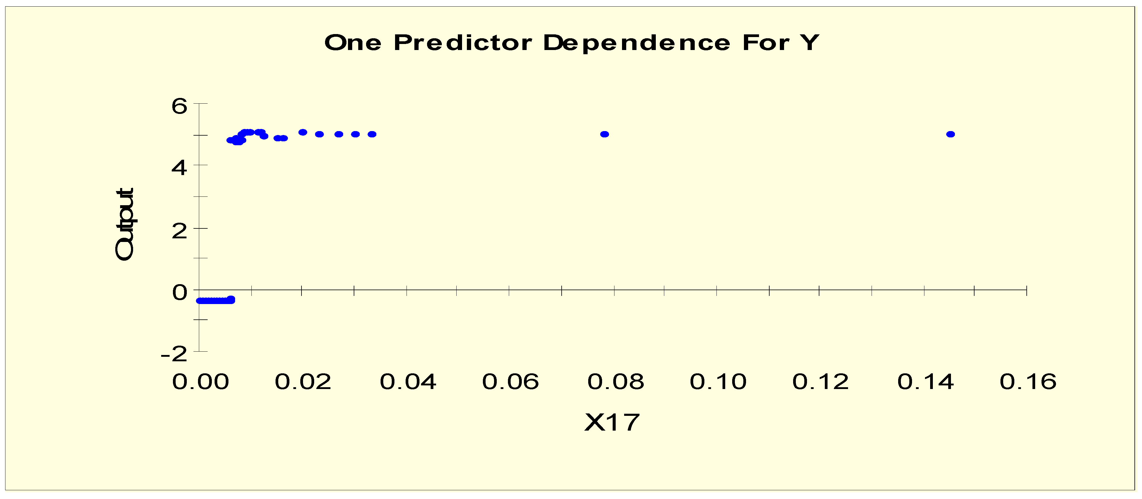
Figure 7 shows the partial dependency plot, which indicates the relationship between TSH (X17) and the log-odds from Model 2. From this plot, we can separate X17 into two levels given that the log-odds value shifts to a different level when X17 = 0.006, i.e., the splitting value is 0.006. The two binary variables, X17LL1 and X17LL2, are generated as shown in Table 6.
Figure 8 shows the partial dependency plot, which indicates the relationship between TT4 (X19) and the log-odds from Model 2. From this plot, we can separate X19 into four levels given that the log-odds value shifts to the different level when X19 = 0.065. Then, the value shows a downward slope when X21 = 0.145. The downward slope stops when X19 = 0.161, and there is no change in the log-odds after this value. Therefore, this predictor is separated into four levels with three splitting values: 0.065, 0.145, and 0.161. The four binary variables, X19LL1, X19LL2, X19LL3, and X19LL4, are generated as shown in Table 6.
Figure 9 shows the partial dependency plot, which indicates the relationship between T3 (X18) and the log-odds from Model 2. From this plot, we can separate X18 into three levels given that it shows a downward slope when X18 = 0.02. The downward slope stops when X18 = 0.045, and there is no change in the log-odds after this value. Therefore, this predictor is separated into three levels with two splitting values, 0.02 and 0.045. The three binary variables, X18LL1, X18LL2, and X18LL3, are generated as shown in Table 6.
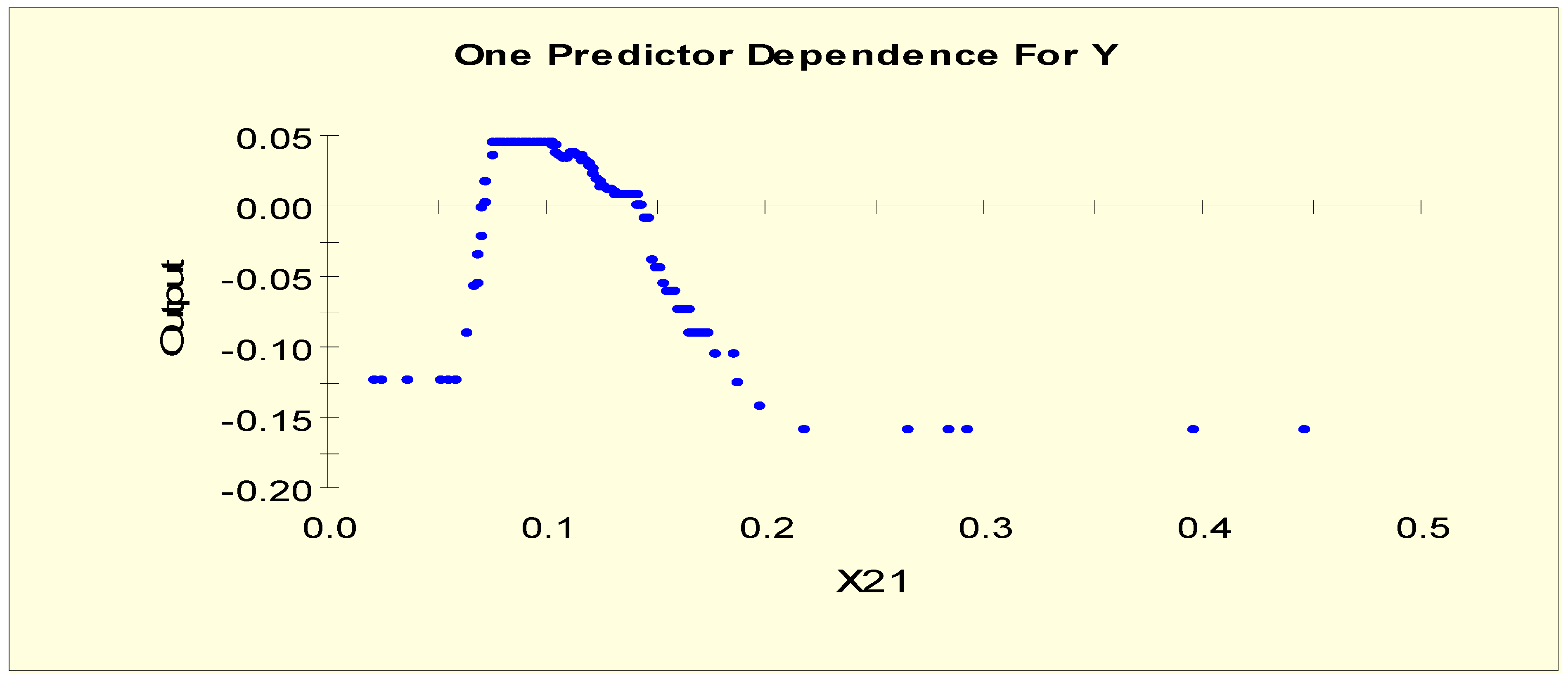
Figure 10 shows the partial dependency plot, which indicates the relationship between FTI (X21) and the log-odds from Model 2. From this plot, we can separate X21 into five levels given that it shows an upward slope when X21 = 0.057. The upward slope stops when X21 = 0.071, and the log-odds value stays constant until X21 = 0.115. Then, the plot shows a downward slope until X21 = 0.217. There is no change in the log-odds after this value. Therefore, this predictor is separated into five levels with four splitting values: 0.057, 0.071, 0.115, and 0.217. The five binary variables, X21LL1, X21LL2, X21LL3, X21LL4, and X21LL5, are generated as shown in Table 6.
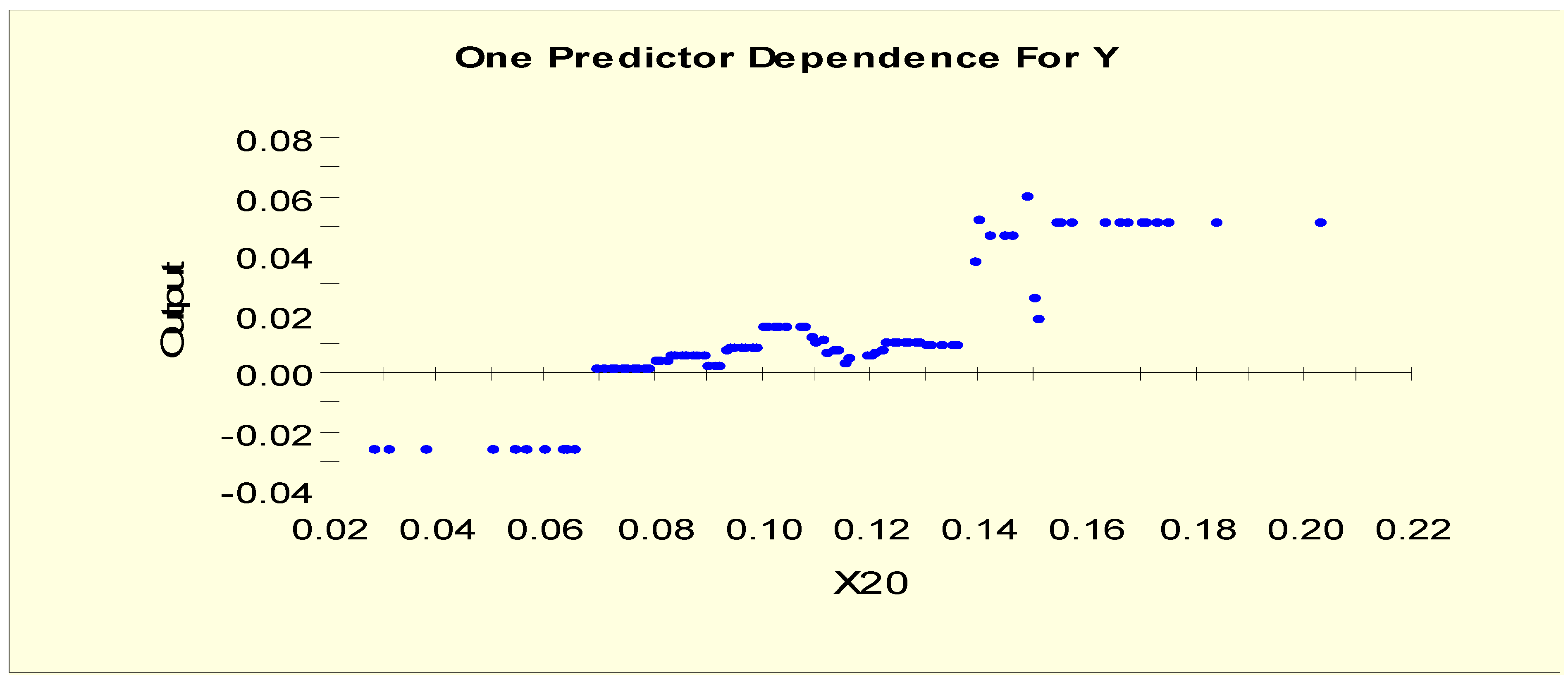
Figure 11 shows the partial dependency plot, which indicates the relationship between T4U (X20) and the log-odds from Model 2. From this plot, we can separate X20 into three levels given that the log-odds value shifts to a different level twice when X20 = 0.07 and when X20 = 0.15, i.e., the splitting values are 0.07 and 0.15. The three binary variables, X20LL1, X20LL2, and X20LL3, are generated as shown in Table 6.
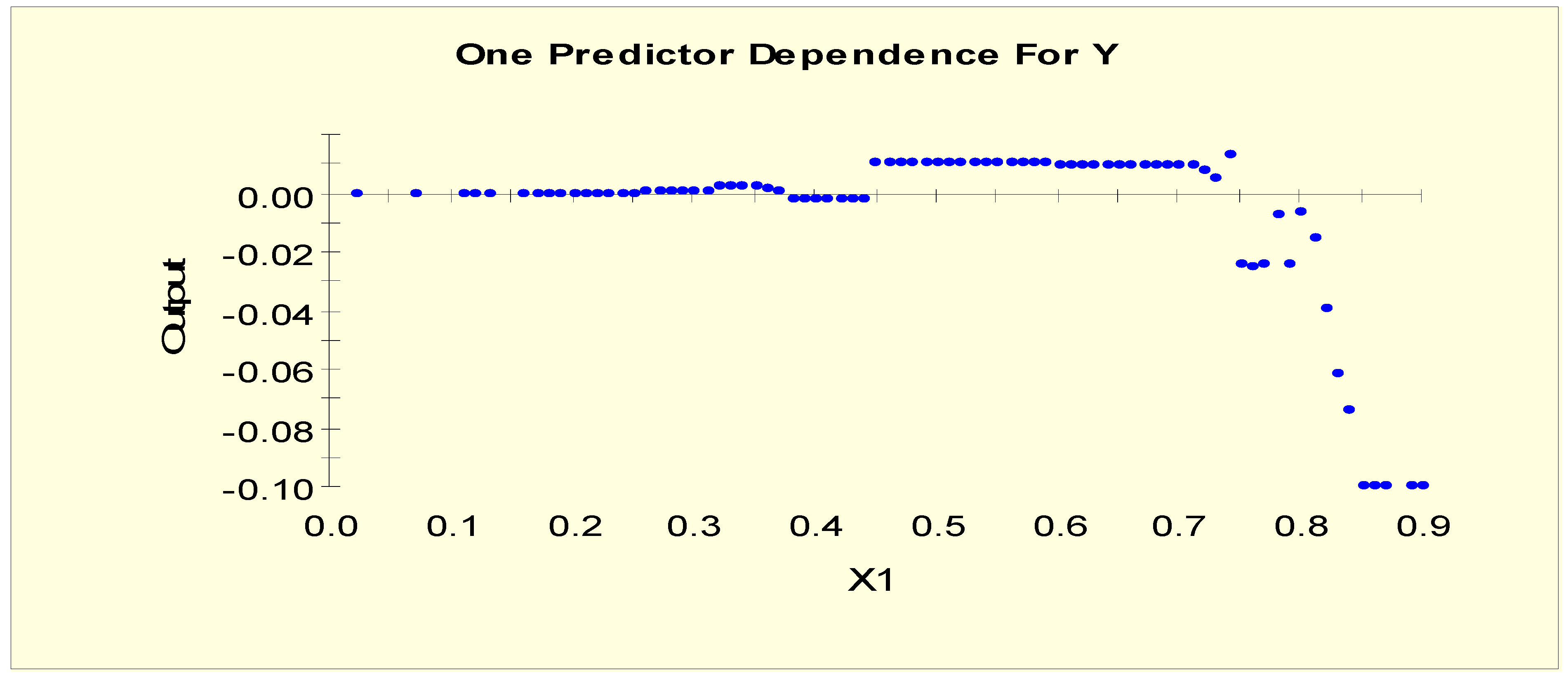
Figure 12 shows the partial dependency plot, which indicates the relationship between age (X1) and log-odds from Model 2. From this plot, there is a downward slope when X1 = 0.75. The downward slope stops when X1 = 0.85, and there is no change in the log-odds after this value. Therefore, this predictor is separated into three levels with two splitting values: 0.75 and 0.85. The three binary variables, X1LL1, X1LL2, and X1LL3, are generated as shown in Table 6.
Note that the second and fourth categories of X4, the third category of X19, the second category of X18, and the second category of X1 all show a linear trend. Therefore, there are five more variables to generate for these five categories (Table 7).
All the variables generated in this step, as shown in Table 3, Table 4, Table 6 and Table 7, serve as the input for building the multinomial model in the final step (step 5). However, only the generated binary variables from Table 3 and Table 6 are included in the input used to search for interactions via ASA in step 2 since ASA can find rules from categorical variables only.
Step 2: Use CBA to obtain the active rules. In this step, the variables input into the process are (i) the original categorical predictors (X2–X16) and (ii) the generated binary variables from Table 3 and Table 6. For this dataset, as the first class (hypo-function) accounts for 2.47% of the dataset, it is necessary to lower the level of support to below 1% in order to capture the rules for this class and set the minimum confidence at 80% to generate the active rules. In total, 5808 rules are generated in this step.
Step 3: Select all the classifier rules from CBA. As a large number of rules are generated in step 2, we take this approach to decrease the number of rules and thereby simplify the process. In total, 26 classifier rules are generated, some examples of which are as follows:
- Rule 6: If X20L1 = 1, X18LL1 = 0, and X21LL4 = 1, then Y = 0 with s = 8.537%, c = 100%.
- Rule 8: If X11 = 0, X19LL3 = 1, and X18LL1 = 0, then Y = 0 with s = 3.075%, c = 100%.
- Rule 22: If X8 = 0, X17L1 = 0, and X19L3 = 0, then Y = 1 with s = 1.935%, c = 97.26%.
- Rule 26: If X3 = 0, X17LL1 = 0, and X19LL2 = 1, then Y = 2 with s = 5.276%, c = 88.945%.
Step 4: Convert the 26 classifier rules into variables. For example, Rule 6 is converted into the new variable referred to as X20L1(1)X18LL1(0)X21LL4(1) and Rule 22 is converted into the new variable referred to as X8(0)X17L1(0)X19L3(0). From 26 classifier rules, we generate 26 interactions. However, two extra variables are generated from Rule 6 and Rule 8. From Model 2, the fourth category of X21 and the third category of X19 each generate a variable, X21QQ4 and X19QQ3, respectively. For Rule 6, as X21LL4 = 1, we generate another interaction, which involves X21QQ4, referred to as X20L1(1)X18LL1(0)X21QQ4. To generate this new variable, we multiply the generated variable X21QQ4 with the dummy variable:
The extra variable from Rule 8 is generated similarly. In total, 28 interactions are generated from the 26 classifier rules.
Step 5: In this illustration, we apply the backward stepwise method and use BIC to select the multinomial logit model. The candidate variables comprise the original variables (X1–X21), all the variables generated from TreeNet, and all 28 potential interactions from step 4.
From the backward stepwise method, we obtain the following model, which yields the best BIC at 233.41. We select this model to represent this dataset, which will be used for classification. To be specific, we will use this model to compute the probability of each patient being in a given class based on the values of the predictors applied. Then, we can assign the most likely class to each patient.
We can further establish the following facts based on the signs and values of the coefficients. The interpretation for the variables generated in Step 2 will be compared to the dependency plots from the TreeNet model, and the interaction generated from step 4 will be compared with the result from ASA:
(i) A patient who is on thyroxine and/or has had thyroid surgery has a higher probability of being in the normal class (Y = 0) than in any of the other classes.
(ii) A patient with an FTI value of 0.07 or higher has a greater probability of being in the normal class (Y = 0) than in the hypo-function class (Y = 1). This result is consistent with the result shown in Figure 2.
(iii) A patient with a TSH value below 0.006 has a greater probability of being in the normal class (Y = 0) than in the hyper-function class (Y = 2). This result is consistent with the result shown in Figure 7.
(iv) A patient with a TT4 value of between 0.065 and 0.145 or a T3 value below 0.02 has a greater probability of being in the hyper-function class (Y = 2) than in the normal class (Y = 0). This result is consistent with the results shown in Figure 8 and Figure 9.
(v) The higher the value of FTI in the range 0.057 to 0.071, the greater the probability of a patient being in the hyper-function class (Y = 2) than in the normal class (Y = 0). This result is consistent with the result shown in Figure 10.
(vi) A patient who has never had thyroid surgery and has a TT4 value below 0.065 and a TSH value of 0.025 or higher has a greater probability of being in the hypo-function class (Y = 1) than in any of the other two classes. This result is consistent with Rule 22.
Our proposed model (Model 3) provides a useful interpretation. However, we will also compare the performance of our model with that of the multinomial logit model developed from different sets of input. As shown in Table 8 Model 1 is the selected multinomial logit model when the candidate predictors comprise only the main effects (X1–X21), whereas Model 2 is the selected multinomial logit model when the candidate predictors comprise the main effects (X1–X21) and all the two-way interactions (X1X2–X20X21, where XiXj = Xi. Xj). Note that all the models are found from stepwise regression using BIC criterion.
4.3. Performance Comparison Using the Training Set
The comparison of the models is based on four criteria: BIC (Bayesian Information Criterion), AIC (Akaike Information Criterion), R2 (McFadden), and accuracy. There are 21 candidate predictors for Model 1, 231 for Model 2, and 90 for Model 3. The comparison shows that for all four criteria, the proposed model (Model 3) outperformed each of the other two models. The misclassification error from our proposed model is only 0.32%, as shown in Table 9.
4.4. Performance Comparison Using the Test Set
For the thyroid dataset, there is a test set comprising 3248 observations of 3178 patients (92.71%) with normal thyroid function, 73 patients (2.13%) with hypo-function, and 177 patients (5.16%) with hyper-function. We applied the eight-variable model (Model 3) obtained from the training set to find the misclassification error from the test set. The misclassification error is only 27 cases out of 3428 cases or 0.79% and the accuracy level is 99.21%, as shown in Table 10.
From Table 9 and Table 10, the proposed method provides very strong predictive ability for both the training set and the test set. We also applied Model 1 and Model 2 with the test set, and the accuracy was 87.51% and 87.95%, respectively.
With this illustration, following our stated approach, we found the model comprising the newly generated variables and the interaction using TreeNet and ASA, i.e., Model 3. This model provides the best fit, very strong predictive ability, and a meaningful interpretation of thyroid disease. Without TreeNet and ASA, this model could not be found.
4.5. Performance Comparison with Other Methodologies
The thyroid dataset has been used for several classification methods, including backpropagation speedup techniques [27], subspace search techniques [28], the local outlier factor and k-nearest neighbors [29].
Schiffmann, Joost, and Werner [27] compared the performance outcomes of 15 backpropagation algorithms for both the training set and test set of the thyroid dataset. Our approach outperforms 14 of these 15 algorithms for both the training and the test sets. The one exception, cascade correlation, has a better classification rate than our approach for the training set but does not perform as well as our approach for the test set. Keller, Müller, and Böhm [28] used the thyroid dataset to compare the performance of five classification methods: the local outlier factor [30], high-contrast subspaces [29], entropy-based subspace clustering [31], ranking interesting subspaces [32], and random subspaces [33]. Our approach outperforms each of these methods and also outperforms the k-nearest neighbors method using average distance as provided by Aggarwal and Sathe [29].
5. Discussion and Conclusions
Our model-building framework advances the multinomial logit model by generating variables and interactions as candidate predictors. We demonstrate that the integration of three techniques—TreeNet, ASA, and the multinomial logit model—constitutes a powerful and practical innovation for data analysis and also paves the way for additional innovative strategies. We have shown via our application example that these newly generated variables and interactions make a significant contribution to improving the multinomial logit model. Our selected model from the thyroid dataset outperforms all of the 21 methods previously applied to the test data.
As illustrated, the approach we propose not only provides superior classification, but also provides a meaningful interpretation of the factors and combinations of factors for thyroid disease. TreeNet eliminates the limitation of the quantitative variables in terms of providing a good fit and generating interactions from ASA. Using the approach described herein, we found that the newly generated variables and the interactions, which are the key to improving the performance of the multinomial logit model, can be found only by using our model-building framework.
Our framework can be applied to many fields to classify multi-level response. However, our focus is on the healthcare field and medical data. Given the consequences of COVID-19, many research studies have been published based on different kinds of modelling with a goal of predicting the prevalence and spread of the disease [34,35,36,37,38]. Our plan in future work is to use our model framework to classify patients with COVID-19 according to levels of severity as a basis for determining the kind of facility at which they should be treated in order to optimize the use of scarce medical resources overall.
Funding
This research received no external funding.
Institutional Review Board Statement
Not applicable.
Informed Consent Statement
Not applicable.
Data Availability Statement
The dataset used for this study can be found at https://archive.ics.uci.edu/ml/datasets/Thyroid+Disease.
Conflicts of Interest
The authors declare no conflict of interest.
References
- Zahid, F.M.; Tutz, G. Multinomial Logit Models with Implicit Variable Selection; Technical Report No. 89; Institute of Statistics, Ludwig-Maximilians-University: Munich, Germany, 2010. [Google Scholar]
- Cherrie, J.A. Variable Screening for Multinomial Logistic Regression on Very Large Data Sets as Applied to Direct Response Modeling. In Proceedings of the SAS Conference Proceedings, SAS Global Forum, Orlando, FL, USA, 16–19 April 2007. [Google Scholar]
- Camminatiello, I.; Lucadamo, A. Estimating multinomial logit model with multicollinearity data. Asian J. Math. Stat. 2010, 3, 93–101. [Google Scholar] [CrossRef]
- Kim, J.H.; Kim, M. Two-stage multinomial logit model. Expert Syst. Appl. 2011, 38, 6439–6446. [Google Scholar] [CrossRef]
- Changpetch, P.; Lin, D.K.J. Selection for multinomial logit models via association rules analysis. WIREs Comput. Stat. 2013, 5, 68–77. [Google Scholar] [CrossRef]
- Introducing TreeNet® Gradient Boosting Machine. Available online: https://www.minitab.com/content/dam/www/en/uploadedfiles/content/products/spm/TreeNet_Documentation.pdf (accessed on 18 February 2020).
- Changpetch, P.; Lin, D.K.J. Model selection for logistic regression via association rules analysis. J. Stat. Comput. Simul. 2013, 83, 1415–1428. [Google Scholar] [CrossRef]
- Agresti, A. Categorical Data Analysis, 2nd ed.; Wiley: Hoboken, NJ, USA, 2020. [Google Scholar]
- Yang, Y.; Webb, G.I. A Comparative Study of Discretization Methods for Naïve-Bayes Classifiers. In Proceedings of the 2002 Pacific Rim Knowledge Acquisition Workshop (PKAW’02), Tokyo, Japan, 18–19 August 2002; Yamaguchi, T., Hoffmann, A., Motoda, H., Compton, P., Eds.; Japanese Society for Artificial Intelligence: Tokyo, Japan, 2002; pp. 159–173. [Google Scholar]
- Catlett, J. On Changing Continuous Attributes into Ordered Discrete Attributes. In Proceedings of the European Working Session on Learning, European Working Session on Learning, Porto, Portugal, 6–8 March 1991; Springer: New York, NY, USA, 1991; pp. 164–178. [Google Scholar]
- Dougherty, J.; Kohavi, R.; Sahami, M. Supervised and Unsupervised Discretization of Continuous Features. In Machine Learning: Proceedings of the Twelfth International Conference on Machine Learning, Tahoe City, CA, USA, 9–12 July 1995; Morgan Kaufmann Publishers: San Francisco, CA, USA, 1995; pp. 194–202. [Google Scholar]
- Kononenko, I. Inductive and Bayesian learning in medical diagnosis. Appl. Artif. Intell. Int. J. 1993, 7, 317–337. [Google Scholar] [CrossRef]
- Kwedlo, W.; Krętowski, M. An Evolutionary Algorithm Using Multivariate Discretization for Decision Rule Induction. In Principles of Data Mining and Knowledge Discovery. PKDD 1999: Lecture Notes in Computer Science, Third European Conference, Prague, Czech Republic, 15–18 September 199; Żytkow, J.M., Rauch, J., Eds.; Springer: Heidelberg/Berlin, Germany, 1999; Volume 1704, pp. 392–397. [Google Scholar]
- Fayyad, U.M.; Irani, K.B. Multi-Interval Discretization of Continuous-Valued Attributes for Classification Learning. In Proceedings of the Thirteenth International Joint Conference on Artificial Intelligence, San Francisco, CA, USA, 28 August–3 September 1993; Morgan Kauffman: Chambéry, France, 1993; Volume 1, pp. 1022–1027. [Google Scholar]
- Pazzani, M.J. An Iterative Improvement Approach for the Discretization of Numeric Attributes in Bayesian Classifiers. In Proceedings of the First International Conference on Knowledge Discovery and Data Mining, Montreal, QC, Canada, 20–21 August 1995; Fayyad, U.M., Uthurusamy, R., Eds.; AAAI Press: Montreal, QC, Canada, 1995; pp. 228–233. [Google Scholar]
- Yang, Y.; Webb, G.I. Proportional k-interval discretization for naive-Bayes classifiers. In Machine Learning: ECML 2001: Lecture Notes in Computer Science, Freiburg, Germany, 5–7 September 2001; De Raedt, L., Flach, P., Eds.; Springer: Heidelberg/Berlin, Germany, 2001; Volume 2167, pp. 228–233. [Google Scholar]
- Hsu, C.N.; Huang, H.J.; Wong, T.T. Why Discretization Works for Naïve Bayesian Classifiers. In Proceedings of the Seventeenth International Conference on Machine Learning, Stanford, CA, USA, 29 June–2 July 2000; Langley, P., Ed.; Morgan Kaufman: San Francisco, CA, USA, 2000; pp. 309–406. [Google Scholar]
- Yang, Y.; Webb, G.I. Non-Disjoint Discretization for Naive-Bayes Classifiers. In Proceedings of the Nineteenth International Conference on Machine Learning (ICML’02), Sydney, Australia, 8–12 July 2002; Sammut, C., Hoffmann, A., Eds.; Morgan Kaufmann: San Francisco, CA, USA, 2002; pp. 666–673. [Google Scholar]
- Yang, Y.; Webb, G.I. Weighted Proportional k-Interval Discretization for Naive-Bayes Classifiers. In Advances in Knowledge Discovery and Data Mining. PAKDD 2003: Lecture Notes in Computer Science, 7th Pacific-Asia Conference, PAKDD, 2003, Seoul, Korea, 30 April 30–2 May 2003; Whang, K.Y., Jeon., J., Shim, K., Srivastava, J., Eds.; Springer: Heidelberg/Berlin, Germany, 2003; Volume 263, pp. 501–512. [Google Scholar]
- Aggarwal, M. On learning of choice models with interactive attributes. IEEE Trans. Knowl. Data Eng. 2016, 28, 2697–2708. [Google Scholar] [CrossRef]
- Berry, M.J.A.; Linoff, G. Data Mining Techniques: For Marketing, Sales, and Customer Support; John Wiley & Sons: New York, NY, USA, 1997. [Google Scholar]
- Agrawal, R.; Srikant, S. Fast Algorithms for Mining Association Rules. In Proceedings of the 20th International Conference on Very Large Data Bases, Santiago, Chile, 12–15 September 1994; Morgan Kaufmann: San Francisco, CA, USA, 1994; pp. 487–499. [Google Scholar]
- Liu, B.; Hsu, W.; Ma, Y. Integrating Classification and Association Rule Mining. In KDD-98 Proceedings of the Fourth International Conference on Knowledge Discovery and Data Mining, New York, NY, USA, 27–31 August 1998; Agrawal, R., Stolorz, P., Piatetsky-Shapiro, G., Eds.; AAAI Press: New York, NY, USA, 1998; pp. 80–86. [Google Scholar]
- Quinlan, J.R. C4.5: Programs for Machine Learning; Morgan Kaufmann: San Francisco, CA, USA, 1992. [Google Scholar]
- Changpetch, P.; Lin, D.K.J. Model selection for Poisson regression via association rules analysis. Internat. J. Stat. Prob. 2015, 4, 1–9. [Google Scholar] [CrossRef] [Green Version]
- Schwarz, G. Estimating the dimension of a model. Ann. Stat. 1978, 6, 461–464. [Google Scholar] [CrossRef]
- Schiffmann, W.; Joost, M.; Werner, R. Optimization of the Backpropagation Algorithm for Training Multilayer Perceptrons; Technical Report; University of Koblenz: Mainz, Germany, 1994. [Google Scholar]
- Keller, F.; Müller, E.; Böhm, K. HiCS: High Contrast Subspaces for Density-Based Outlier Ranking. In Proceedings of the 2012 IEEE 28th International Conference on Data Engineering (ICDE’12), Arlington, VA, USA, 1–5 April 2012; pp. 1037–1048. [Google Scholar]
- Aggarwal, C.C.; Sathe, S. Theoretical foundations and algorithms for outlier ensembles. SIGKDD Explor. Newsl. 2015, 17, 24–47. [Google Scholar] [CrossRef]
- Breunig, M.M.; Kriegel, H.; Ng, R.T.; Sander, J. LOF: Identifying Density-Based Local Outliers. In Proceedings of the 2000 ACM SIGMOD International Conference on Management of Data (SIGMOD’00), Dallas, TX, USA, 16–18 May 2000; ACM: New York, NY, USA, 2000; pp. 93–104. [Google Scholar]
- Cheng, C.; Fu, A.W.; Zhang, Y. Entropy-Based Subspace Clustering for Mining Numerical Data. In Proceedings of the Fifth ACM SIGKDD International Conference on Knowledge Discovery and Data Mining (KDD’99), San Diego, CA, USA, 15–18 August 1999; ACM: New York, NY, USA, 1999; pp. 84–93. [Google Scholar]
- Kailing, K.; Kriegel, H.P.; Kröger, P.; Wanka, S. Ranking Interesting Subspaces for Clustering High Dimensional Data. In Knowledge Discovery in Databases: PKDD 2003: Lecture Notes in Computer Science, PKDD 2003, 7th European Conference on Principles and Practice of Knowledge Discovery in Databases, Cavtat-Dubrovnik, Croatia, 22–26 September 2003; Lavrač, N., Gamberger, D., Todorovski, L., Blockeel, H., Eds.; Springer: Berlin/Heidelberg, Germany, 2003; Volume 2838, pp. 241–253. [Google Scholar]
- Skurichina, M.; Duin, R.P.W. Bagging, boosting and the random subspace method for linear classifiers. Pattern Anal. Appl. 2002, 5, 121–135. [Google Scholar] [CrossRef]
- Ceylan, Z. Estimation of COVID-19 prevalence in Italy, Spain, and France. Sci. Total Environ. 2020, 729, 138817. [Google Scholar] [CrossRef]
- Lukman, A.F.; Rauf, R.I.; Abiodun, O.; Oludoun, O.; Ayinde, K.; Ogundokun, R.O. COVID-19 prevalence estimation: Four most affected African countries. Infect. Dis. Model. 2020, 5, 827–838. [Google Scholar] [CrossRef] [PubMed]
- Benvenuto, D.; Giovanetti, M.; Vassallo, L.; Angeletti, S.; Ciccozzi, M. Application of the ARIMA model on the COVID-2019 epidemic dataset. Data Brief. 2020, 29, 105340. [Google Scholar] [CrossRef] [PubMed]
- La Gatta, V.; Moscato, V.; Postiglione, M.; Sperli, G. An epidemiological neural network exploiting dynamic graph structured data applied to the covid-19 outbreak. IEEE Trans. Big Data 2020, 14. [Google Scholar] [CrossRef]
- Varotsos, C.A.; Krapivin, V.F. A new model for the spread of COVID-19 and the improvement of safety. Safety Sci. 2020, 132, 104962. [Google Scholar] [CrossRef]
Figure 1.
Partial dependence plot of TSH (X17).

Figure 2.
Partial dependence plot of FTI (X21).

Figure 3.
Partial dependence plot of TT4 (X19).

Figure 4.
Partial dependence plot of T3 (X18).

Figure 5.
Partial dependence plot of T4U (X20).

Figure 6.
Partial dependence plot of age (X1).

Figure 7.
Partial dependence plot of TSH (X17).

Figure 8.
Partial dependence plot of TT4 (X19).

Figure 9.
Partial dependence plot of T3 (X18).

Figure 10.
Partial dependence plot of FTI (X21).

Figure 11.
Partial dependence plot of T4U (X20).

Figure 12.
Partial dependence plot of age (X1).


Table 1.
Predictors for the thyroid dataset.
| Attribute | Description | Variable |
|---|---|---|
| Age | Age in years | X1 |
| Sex | Gender | X2 = 1 if male and X2 = 0 if female |
| On Thyroxine | Patient on Thyroxine | X3 = 1 if yes and X3 = 0 if no |
| Query Thyroxine | Maybe on Thyroxine | X4 = 1 if yes and X4 = 0 if no |
| On antithyroid | On antithyroid medication | X5 = 1 if yes and X5 = 0 if no |
| Sick | Patient reports malaise | X6 = 1 if yes and X6 = 0 if no |
| Pregnant | Patient pregnant | X7 = 1 if yes and X7 = 0 if no |
| Thyroid surgery | History of thyroid surgery | X8 = 1 if yes and X8 = 0 if no |
| I131 treatment | Patient on I131 treatment | X9 = 1 if yes and X9 = 0 if no |
| Query hypothyroid | Maybe hypothyroid | X10 = 1 if yes and X10 = 0 if no |
| Query hyperthyroid | Maybe hyperthyroid | X11 = 1 if yes and X11 = 0 if no |
| Lithium | Patient on lithium | X12 = 1 if yes and X12 = 0 if no |
| Goiter | Patient has goiter | X13 = 1 if yes and X13 = 0 if no |
| Tumor | Patient has tumor | X14 = 1 if yes and X14 = 0 if no |
| Hypopituitary | Patient hypopituitary | X15 = 1 if yes and X15 = 0 if no |
| Psych | Psychological symptoms | X16 = 1 if yes and X16 = 0 if no |
| Thyroid Stimulating Hormone (TSH) | TSH value, if measured | X17 |
| Triiodothyronine (T3) | T3 value, if measured | X18 |
| Total Thyroxine (TT4) | TT4 value, if measured | X19 |
| Thyroxine Uptake (T4U) | T4U value, if measured | X20 |
| Free Thyroxine Index (FTI) | FTI—calculated from TT4 and T4U | X21 |
Table 2.
Variable importance plot for Model 1.
| Variable | Score | |
|---|---|---|
| X17 | 100.00 | |||||||||||||||||||||||||||||||||||||||||| |
| X21 | 63.88 | |||||||||||||||||||||||||| |
| X8 | 25.08 | |||||||||| |
| X3 | 17.38 | |||||| |
| X19 | 12.16 | |||| |
| X18 | 6.67 | || |
| X20 | 6.56 | || |
| X2 | 6.42 | || |
| X1 | 3.11 | |
| X10 | 2.71 | |
| X9 | 2.00 | |
| X11 | 1.93 |
Table 3.
Generated binary variables.
| Original Variables | Generated Binary Variables |
|---|---|
| TSH (X17) | X17L1 = 1 if X17 < 0.025 and X17L1 = 0 otherwise |
| X17L2 = 1 if 0.025 ≤ X17 and X17L2 = 0 otherwise | |
| FTI (X21) | X21L1 = 1 if X21 < 0.055 and X21L1 = 0 otherwise |
| X21L2 = 1 if 0.055 ≤ X21 < 0.07 and X21L2 = 0 otherwise | |
| X21L3 = 1 if 0.07 ≤ X21 and X21L3 = 0 otherwise | |
| TT4 (X19) | X19L1 = 1 if X19 < 0.042 and X19L1 = 0 otherwise |
| X19L2 = 1 if 0.042 ≤ X19 < 0.065 and X19L2 = 0 otherwise | |
| X19L3 = 1 if 0.065 ≤ X19 and X19L3 = 0 otherwise | |
| T3 (X18) | X18L1 = 1 if X18 < 0.006 and X18L1 = 0 otherwise |
| X18L2 = 1 if 0.006 ≤ X18 and X18L2 = 0 otherwise | |
| T4U (X20) | X20L1 = 1 if X20 < 0.097 and X20L1 = 0 otherwise |
| X20L2 = 1 if 0.097 ≤ X20 and X20L2 = 0 otherwise | |
| Age (X1) | X1L1 = 1 if X1 < 0.15 and X1L1 = 0 otherwise |
| X1L2 = 1 if 0.15 ≤ X1 and X1L2 = 0 otherwise |
Table 4.
Generated variables with linear trend.
| Original Variables | Generated Variables with Linear Trend |
|---|---|
| FT1 (X21) | X21Q2 = X21 if 0.055 ≤ X21 < 0.07 and X21Q2 = 0 otherwise |
| TT4 (X19) | X19Q2 = X19 if 0.042 ≤ X19 < 0.065 and X19Q2 = 0 otherwise |
Table 5.
Variable importance plot for Model 2.
| Variable | Score | |
|---|---|---|
| X17 | 100.00 | |||||||||||||||||||||||||||||||||||||||||| |
| X3 | 44.88 | |||||||||||||||||| |
| X8 | 25.20 | |||||||||| |
| X19 | 22.47 | ||||||||| |
| X18 | 17.51 | ||||||| |
| X21 | 10.87 | |||| |
| X20 | 8.04 | || |
| X1 | 6.68 | || |
| X10 | 5.15 | | |
| X5 | 4.21 | | |
| X12 | 4.02 | | |
| X11 | 3.20 | |
| X2 | 0.84 |
Table 6.
Generated binary variables.
| Original Variables | Generated Binary Variables |
|---|---|
| TSH (X17) | X17LL1 = 1 if X17 < 0.006 and X17LL1 = 0 otherwise |
| X17LL2 = 1 if 0.006 ≤ X17 and X17LL2 = 0 otherwise | |
| FTI (X21) | X21LL1 = 1 if X21 < 0.057 and X21LL1 = 0 otherwise |
| X21LL2 = 1 if 0.057 ≤ X21 < 0.071 and X21LL2 = 0 otherwise | |
| X21LL3 = 1 if 0.071 ≤ X21 < 0.115 and X21LL3 = 0 otherwise | |
| X21LL4 = 1 if 0.115 ≤ X21 < 0.217 and X21LL4 = 0 otherwise | |
| X21LL5 = 1 if 0.217 ≤ X21 and X21LL5 = 0 otherwise | |
| TT4 (X19) | X19LL1 = 1 if X19 < 0.065 and X19LL1 = 0 otherwise |
| X19LL2 = 1 if 0.065 ≤ X19 < 0.145 and X19LL2 = 0 otherwise | |
| X19LL3 = 1 if 0.145 ≤ X19 < 0.161 and X19LL3 = 0 otherwise | |
| X19LL4 = 1 if 0.161 ≤ X19 and X19LL4 = 0 otherwise | |
| T3 (X18) | X18LL1 = 1 if X18 < 0.02 and X18LL1 = 0 otherwise |
| X18LL2 = 1 if 0.02 ≤ X18 < 0.045 and X18LL2 = 0 otherwise | |
| X18LL3 = 1 if 0.045 ≤ X18 and X18LL3 = 0 otherwise | |
| T4U (X20) | X20LL1 = 1 if X20 < 0.07 and X20LL1 = 0 otherwise |
| X20LL2 = 1 if 0.07 ≤ X20 < 0.15 and X20LL2 = 0 otherwise | |
| X20LL3 = 1 if 0.15 ≤ X20 and X20LL3 = 0 otherwise | |
| Age (X1) | X1LL1 = 1 if X1 < 0.75 and X1LL1 = 0 otherwise |
| X1LL2 = 1 if 0.75 ≤ X1< 0.85 and X1LL2 = 0 otherwise | |
| X1LL3 = 1 if 0.85 ≤ X1 and X1LL3 = 0 otherwise |
Table 7.
Generated variables with linear trend.
| Original Variables | Generated Variables with Linear Trend |
|---|---|
| FT1 (X21) | X21QQ2 = X21 if 0.057 ≤ X21 < 0.071 and X21QQ2 = 0 otherwise |
| X21QQ4 = X21 if 0.115 ≤ X21 < 0.217 and X21QQ4 = 0 otherwise | |
| TT4 (X19) | X19QQ3 = X19 if 0.145 ≤ X19 < 0.161 and X19QQ3 = 0 otherwise |
| T3 (X18) | X18QQ2 = X18 if 0.02 ≤ X18 < 0.045 and X18QQ2 = 0 otherwise |
| Age (X1) | X1QQ2 = X1 if 0.75 ≤ X1< 0.85 and X1QQ2 = 0 otherwise |
Table 8.
Model comparison.
| Model | Candidate Predictors | BIC | AIC | R2 (McFadden) | Accuracy |
|---|---|---|---|---|---|
| Model 1 | Main effects (X1–X21) | 916.05 | 841.23 | 65.58% | 97.03% |
| Model 2 | Main effects (X1–X21) All two-way interactions | 561.56 | 449.32 | 82.59% | 98.36% |
| Model 3 | Main effects (X1–X21) Generated variables from step 2 Generated interactions from step 4 | 233.41 | 121.17 | 96.41% | 99.68% |
Table 9.
Misclassification from Model 3.
| Actual Class | ||||
|---|---|---|---|---|
| 0 | 1 | 2 | ||
| Predict class | 0 | 3479 | 2 | 1 |
| 1 | 3 | 91 | 0 | |
| 2 | 6 | 0 | 190 | |
Table 10.
Misclassification from Model 3 applied to the test set.
| Actual Class | ||||
|---|---|---|---|---|
| 0 | 1 | 2 | ||
| Predict class | 0 | 3165 | 6 | 8 |
| 1 | 4 | 67 | 0 | |
| 2 | 9 | 0 | 169 | |
Publisher’s Note: MDPI stays neutral with regard to jurisdictional claims in published maps and institutional affiliations. |
© 2021 by the author. Licensee MDPI, Basel, Switzerland. This article is an open access article distributed under the terms and conditions of the Creative Commons Attribution (CC BY) license (http://creativecommons.org/licenses/by/4.0/).
Share and Cite
MDPI and ACS Style
Changpetch, P. Multinomial Logit Model Building via TreeNet and Association Rules Analysis: An Application via a Thyroid Dataset. Symmetry 2021, 13, 287. https://0-doi-org.brum.beds.ac.uk/10.3390/sym13020287
AMA Style
Changpetch P. Multinomial Logit Model Building via TreeNet and Association Rules Analysis: An Application via a Thyroid Dataset. Symmetry. 2021; 13(2):287. https://0-doi-org.brum.beds.ac.uk/10.3390/sym13020287
Chicago/Turabian StyleChangpetch, Pannapa. 2021. "Multinomial Logit Model Building via TreeNet and Association Rules Analysis: An Application via a Thyroid Dataset" Symmetry 13, no. 2: 287. https://0-doi-org.brum.beds.ac.uk/10.3390/sym13020287
Note that from the first issue of 2016, this journal uses article numbers instead of page numbers. See further details here.