
Bifurcation Analysis of Time-Delay Model of Consumer with the Advertising Effect


1
Zhengzhou Key Laboratory of Big Data Analysis and Application, Henan Academy of Big Data, Zhengzhou University, Zhengzhou 450052, China
2
Department of Mathematics, College of Science, King Khalid University, P.O. Box 9004, Abha 61413, Saudi Arabia
3
Department of Mathematics, Faculty of Science, Al-Azhar University, Assiut branch, Assiut 71524, Egypt
4
Section of Mathematics, Università Telematica Internazionale Uninettuno, 00186 Rome, Italy
*
Author to whom correspondence should be addressed.
Symmetry 2021, 13(3), 417; https://0-doi-org.brum.beds.ac.uk/10.3390/sym13030417
Submission received: 14 February 2021
/
Revised: 22 February 2021
/
Accepted: 24 February 2021
/
Published: 4 March 2021
(This article belongs to the Special Issue Complex Variable in Approximation Theory)
Abstract
:Given the economic importance of advertising and product promotions, we have developed a diffusion model to describe the impact of advertising on sales. The main message of this study is to show the effect of advertising diffusion to convert potential buyers into actual customers which may result in persistent alteration in marketing over time. This work is devoted to studying the dynamic behavior of a reaction-diffusion model and its delayed version with the advertising effect. For the non-delay model, it is proven the existence of Hopf bifurcation. Moreover, the stability and direction of bifurcation of periodic solutions are detected. On the other hand, we consider there is a lag for responding of potential buyers to the advertising. Therefore, the time delay is deemed as an additional factor in the diffusion model. We have determined the critical values for the delay parameter that yield periodic solutions. Furthermore, the direction and the stability of bifurcating periodic solutions is studied. For supporting the theoretical analysis and demonstrate complex dynamic behaviors, numerical simulations including families of periodic curves are given.
1. Introduction
Advertising has an important role in our life. It mainly affects the determination of the image and method of purchase, and it also affects our thinking towards different and new products. Advertising is connected with brand recognition and choosing measures to build the commercial long-term strategy, while promotion activities are seasonal measures to raise the company’s immediate revenues by directly influence the prices of goods or services.
In view of the economic importance of advertising promotion, it has been discussed in many economic and social studies. In [1], how advertising creativity influences consumer treatment and response has been discussed. In [2], the effect of advertising bans has been studied to limit the spread of tobacco products. However, the results proved the effectiveness of advertising bans on the consumption of tobacco products. In [3], the effect of word of mouth on consumer marketing behavior was examined based on preliminary data collected from the population of some cities, and the results revealed the effect of word of mouth on marketing of various commercial products. For more information and results see [4,5].
Many studies have used the innovation diffusion theory since its appearance due to its great economic importance. Numerous mathematical models have been established to market new products. Sales promotions have been widely discussed in many studies from both mathematical and economic standpoints. Many of these models have been developed to clarify the diffusion of the products amongst potential customers of the population, by taking into account the influence of oral speech, advertising and other means of communication. Since then, these models have been studied and developed in several research perspectives which resulting in important theoretically and practically contributions.
To name a few, we can highlight some of the described diffusion models. In [6], Bass has developed a growth model describing successive purchases by assuming that the number of previous purchases affect the purchase expectations. Which led to good predictions of buying behavior consistent with experimental data. In [7], Dodson and etc. have been developed a model for the interaction process between adopters and non-adopters and the effect of repetitive purchase. Hence, the behavioral assumptions that support the model are clarified.
In [8], Australian scholar Feichtinger established a two-dimensional advertising diffusion model as follows:
where are the number of potential buyers of a specific brand at time t and customers of this brand at that time, respectively. The coefficients in model (1) are illustrated in Table 1.
In [9], it has been considered the impact of product marketing planning on potential consumers to improve Feichtinger’s model by
where c indicates the success rate of marketing planning. In [10], a mathematical model to interpret consumer behavior under the advertising and word-of-mouth effects was proposed, which was studied in both of continuous and discrete versions, for more studies see [11,12].
The theory of dynamism applied to behavior allows us to study and analyze this movement between the condition of current client and the potential one. The trajectory in time that reflects the evolution of both types of clients and their role change can be analyzed by studying the bifurcations of the dynamic model, since they reflect a change in the behavior of the elements studied. The analysis of the independent variables controlled by the organization and the sensitivity of the parametric values that reflect the trend in behavioral changes make it possible to visualize the possible movements in the system.
Recently, the differential equations theory (stability, bifurcation, chaos, etc.) has been used in several fields such as medicine, economics, life science, engineering, technology and sociology [13,14,15,16,17].
The analysis of time-delay differential equations is more realistic to describe the interactions between elements of dynamic systems. The time delays can be regarding to the period of some hidden processes, such as the stages of growth, response and sensitivity to some influences, and the incubation period of the infectious diseases [18,19,20,21,22].
Given the economic importance of the impact of revenue on daily life, we investigate the dynamic behaviors of the effect of ads to give a clearer view and to reveal the influencing factors. Based on [8], in our paper we consider a clear three compartment model which consists of the numbers of potential and actual consumers and the influence of advertising. In modification of [8], we consider that the dynamics of the potential buyers number and buyers are influenced by the advertising effect in Holling type I.
The rest of our article is regulated as follows. Section 2 provides the mathematical model and the equilibria existence. In Section 3 and Section 4 we analyze the dynamical behavior of continuous consumption behavior model and delayed consumption behavior model, respectively, including the numerical simulations. In the last, we conclude the paper with a brief discussion in Section 5.
2. The Mathematical Model and Its Dynamics
Advertising can affect a company’s sales volume in both the short and long term, contingent upon its targets. It is assumed that the rate of the conversion of potential buyers to customers, is proportional to the advertisements effect function. Suppose the advertisement stimulates the increase in the number of consumers represented by the positive nonlinear growth term for potential buyers, which can be conveniently represented by the response function Holling Type 2. Based on description of the dissemination of advertising in [23] the change of advertising influence over time can be described by the logistic curve.
Thus, the flows of individuals are divided into the two different groups and and the influence of advertising . can be presented as follows:
where a is the half-saturation constant and b is the response rate of the individuals, , and are control parameters of logistics curve.
To simplify calculations, we carry out the following transformations:
and
For avoiding the abuse of mathematical notation, we still denote by , system (2) becomes
where , .
Due to the previous transformations, systems (2) and (3) are topologically equivalent, so we are going to study system (3) instead of the original system.
Proposition 1.
The following triples are all equilibrium points of system (3)
- 1.
- Semi-trivial equilibrium point ,
- 2.
- Nontrivial equilibrium , where .
The Jacobian matrix of system (3) at takes the form
therefore, the characteristic equation is expressed as [24]
Which leads to a non negative eigenvalue and the other two eigenvalues satisfy the following equation
Lemma 1.
The eigenvalues of satisfy the following conditions
- 1.
- iff ;
- 2.
- iff ;
- 3.
- and iff ;
- 4.
- iff .
The Jacobian matrix of system (3) at takes the form
therefore, the characteristic equation can be written as
where , .
One can verify is always a non positive eigenvalue, the other two eigenvalues satisfy the following equation
Lemma 2.
The eigenvalues of satisfy the following conditions
- 1.
- iff ;
- 2.
- iff ;
- 3.
- and iff ;
- 4.
- iff .
Theorem 1.
The semi-trivial equilibrium point is
- 1.
- A hyperbolic saddle if ;
- 2.
- An unstable Equilibrium Point if ;
- 3.
- A non-hyperbolic point if the parameter satisfies one of the following conditions
- (a)
- ;
- (b)
- .
Theorem 2.
The non-trivial equilibrium point is
- 1.
- A hyperbolic saddle if ;
- 2.
- A stable Equilibrium Point if ;
- 3.
- A non-hyperbolic Equilibrium Point if .
3. Stability and Bifurcation Analysis
In this part, we investigate the topological equivalent system (3) of the original system and analyze the bifurcation.
3.1. Hopf Bifurcation of Semi-Trivial Equilibrium Point
Theorem 3.
System (8) undergoes Hopf at if .
Proof.
From (5), one can get the eigenvalues of of system (3) as follows:
To verify the transversality condition. Consider the real part of the complex eigenvalues of the characteristic equation . Let be the bifurcation parameter, then suppose that implies
Therefore, the eigenvalues of the system (8) become
where i denotes an imaginary unit. The transversality condition can be verified as
Hence, system (8) undergoes Hopf bifurcation. □
Next, the normal form theory is useful to study the direction and stability of bifurcating periodic solutions for system (8) [26]. Let the eigenvectors corresponding to the eigenvalues and be and , where and are real vectors.
By straightforward calculations, we obtain
Define
By straightforward calculations, we get
where
Then, following a similar computation process as in [15] we can calculate the first Lyapunov coefficient of system (3),
and
For classifying the existence of a generic Hopf bifurcation
3.2. Hopf Bifurcation of Non-Trivial Equilibrium Point
Next, we study the bifurcation analysis of system (3) at the equilibrium point . By applying the theory of series at the point , system (3) can be presented as
For system (3), let , then system (12) becomes
where
,
.
Theorem 4.
A bifurcation occurs at if and .
Proof.
As we did in the previous subsection we can get to determine the direction of Hopf bifurcation.
3.3. Numerical Simulations
In this part, a rigorous investigation of the influenced advertising diffusion model by word-of-mouth response to verify the analytical result numerically. The dynamics of system is explored using both of the software packages MATLAB and AUTO by varying different parameters. We select some parameters values to illustrate the existence of the Hopf bifurcation in different equilibrium points. For satisfying the bifurcation conditions, we select the parameters as and as a bifurcation parameter. The illustrative simulations are shown as following.
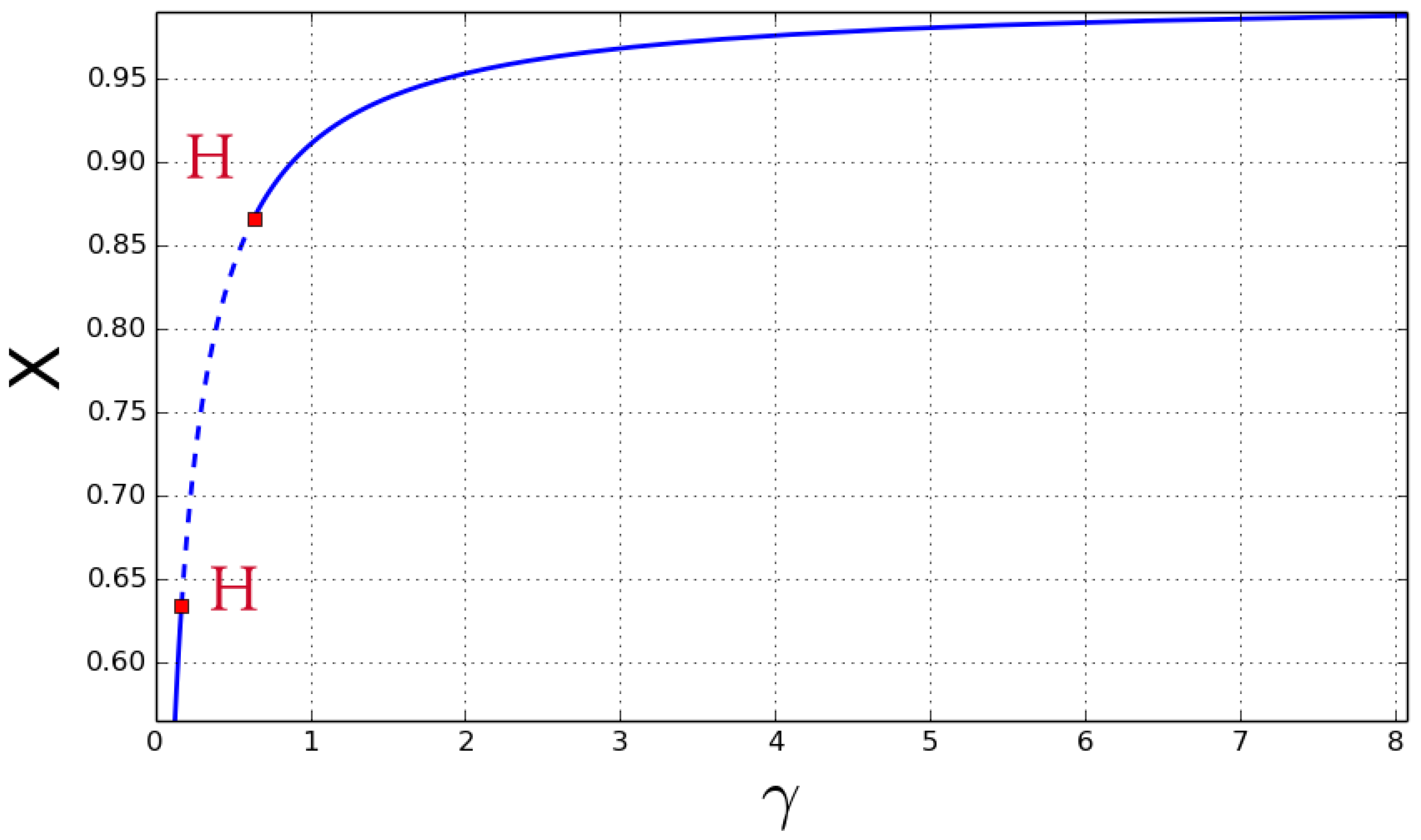
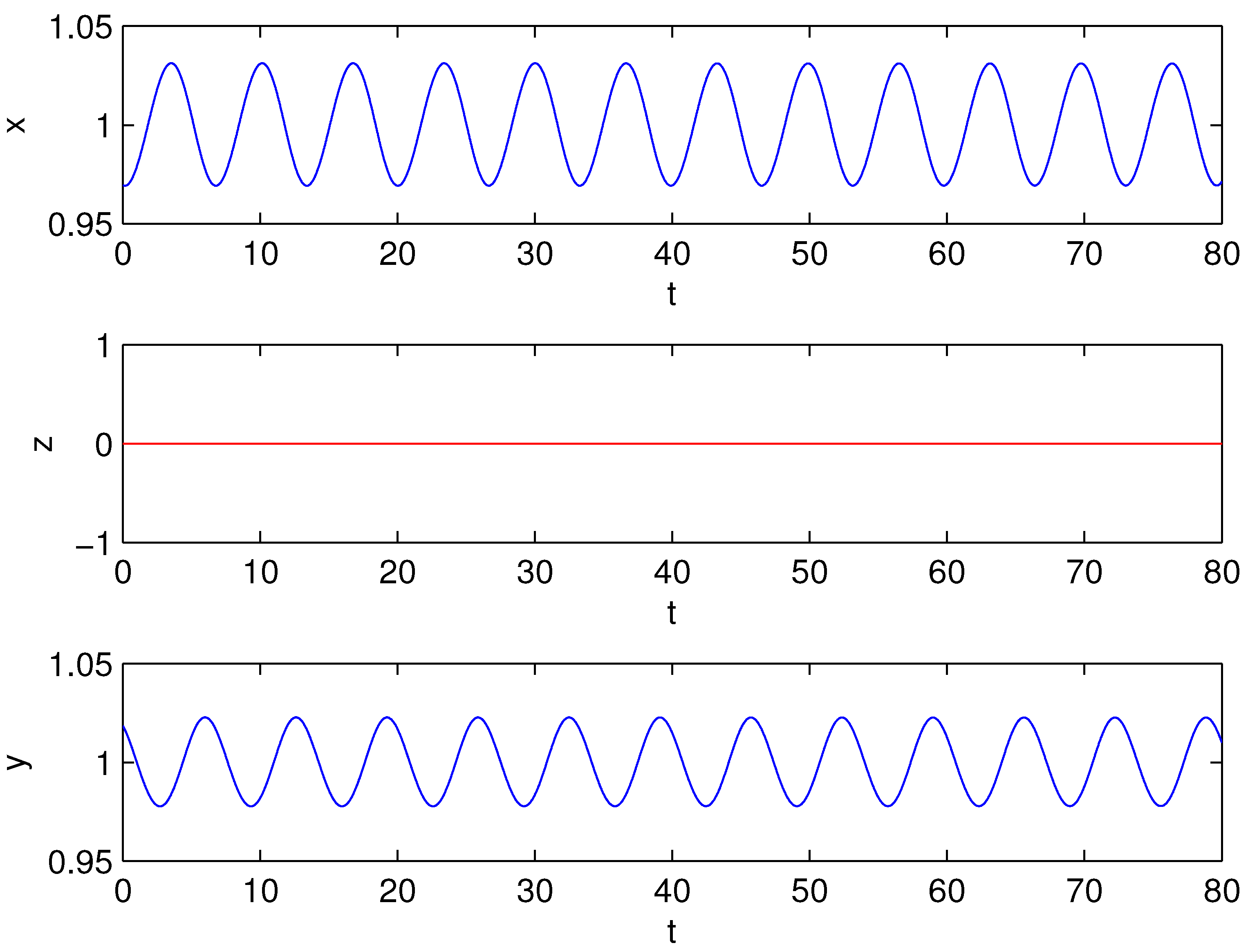
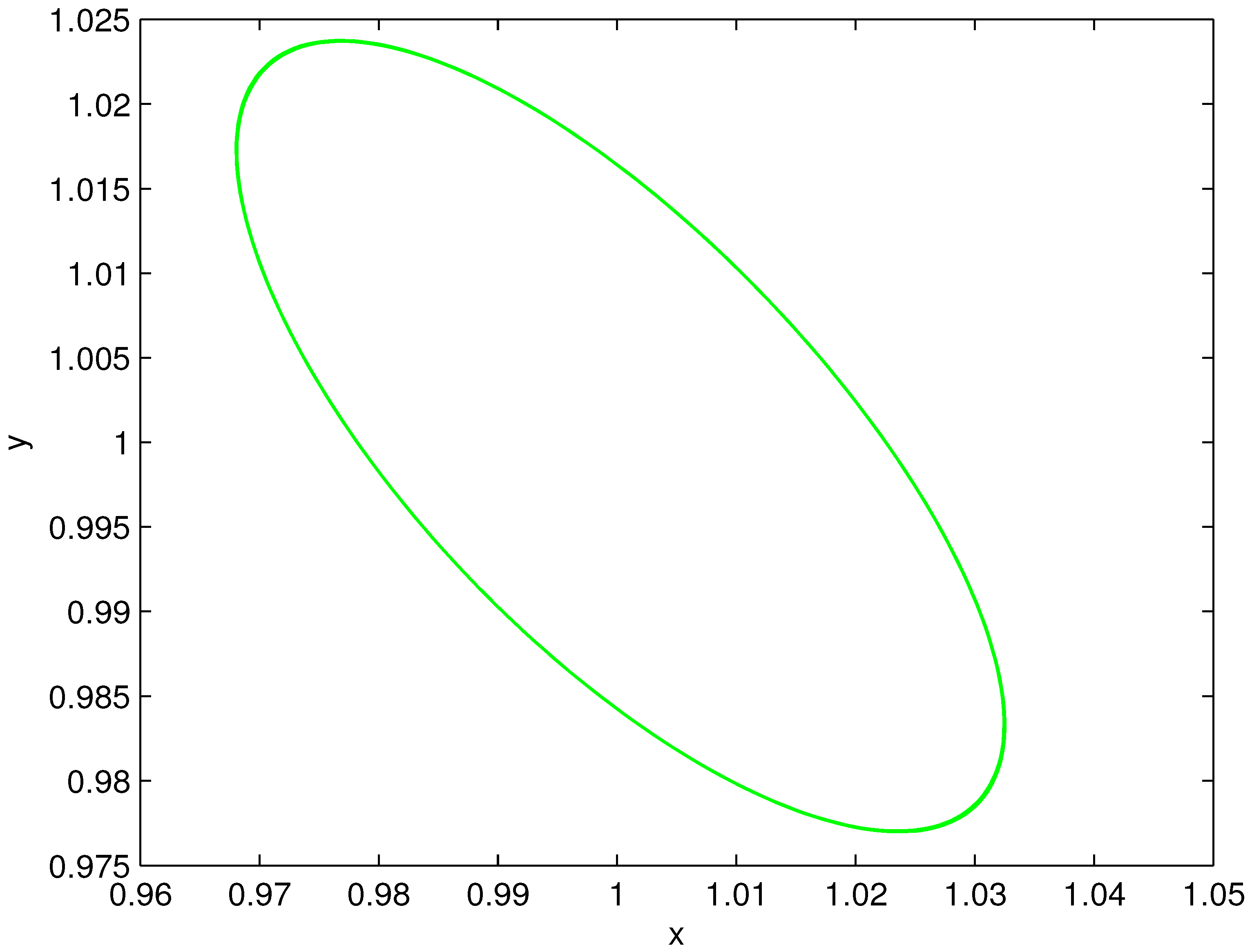
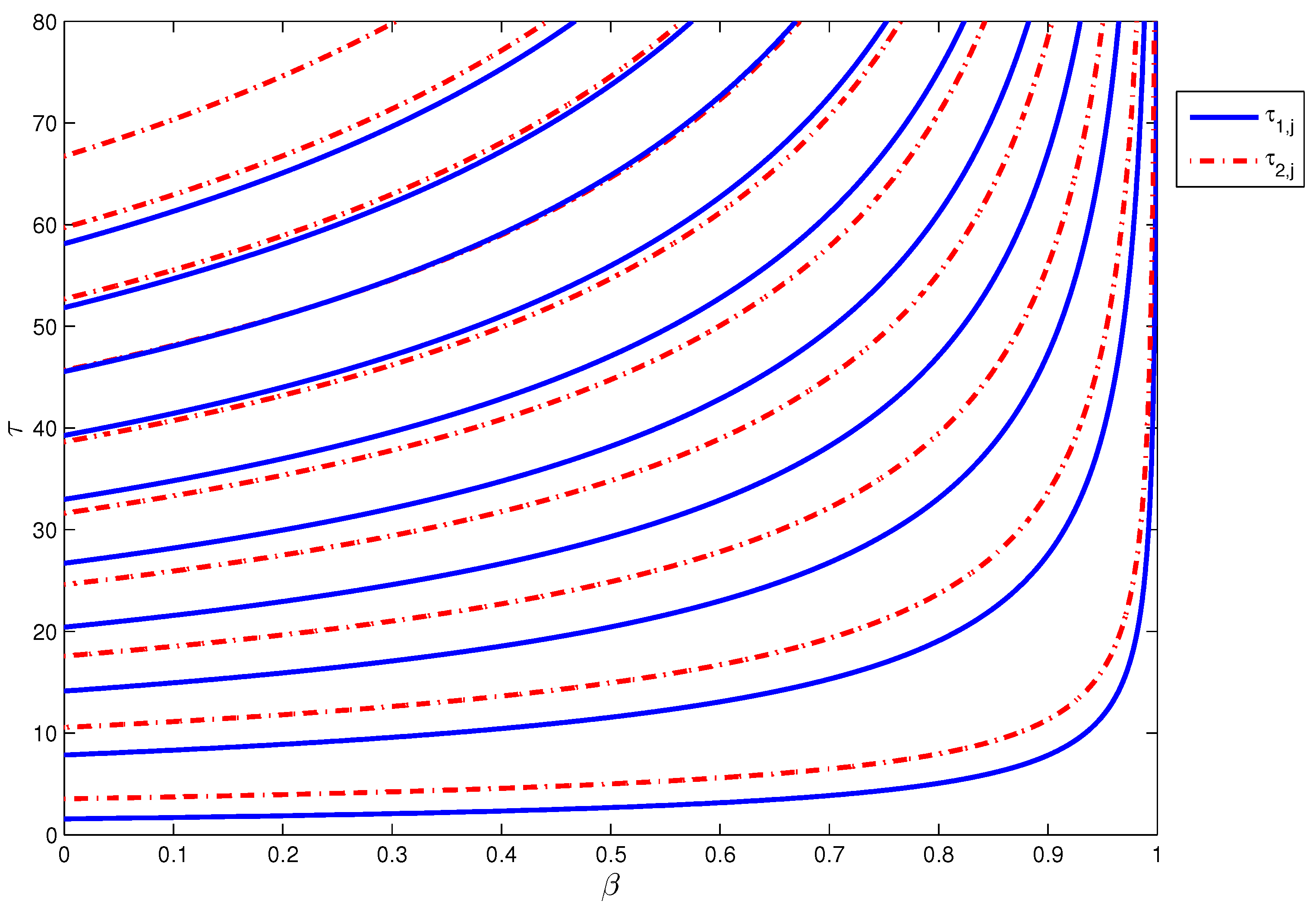
Figure 1 and Figure 2 show the values of at which Hopf bifurcation occurs. It can be seen from Figure 1 that Hopf bifurcation occurs at at one value , while there are two values at . Some phase portraits and time series of limit cycle are given in Figure 3 and Figure 4 at and in Figure 5, Figure 6, Figure 7 and Figure 8 at . By the computation of the AUTO package, we present all the first Lyapunov coefficient of the Hopf points in Table 2.
4. Delayed Model and Its Dynamics
Taking into account that the effect of advertising in the non-potential buyers class most probably does not happen instantaneously, it is assumed that the potential buyers takes time for reacting with the advertising. In other words, it is presumed that there is a time delayed in the response of potential buyers to purchase the product under the influence of advertising. Thus, the proportion of potential buyers who became customers due to advertising is . Consequently, the delayed model of (3) is given by
By applying the theory of series at the point , system (14) can be expressed as
4.1. Stability of Equilibria and Bifurcations of Periodic Solutions
Now, we analyze the delay effect on the dynamic behavior of system (15). When , system (15) returns to the system (3), which has been studied in the previous sections.
Obviously, the equilibria of system (3) still the same for the delayed system (15). From proposition (1), system (15) has two equilibria as well. Through the next transformation
The linearized system (15) becomes:
which can be written as
where,
The characteristic polynomial of the delayed system (15), depending on , is expressed as follows:
A straightforward calculation leads to
where
Obviously, is constantly an eigenvalue and the remain eigenvalues satisfy the following equation
Therefore, we analyze the distribution of the roots of Equation (19).
For has roots with negative real parts iff
where
Now, we consider . For the occurrence of the Hopf bifurcation, denote is the eigenvalue of the characteristic Equation (19), where and depend on the delay . A critical time delay must exist such that and the transversally condition is satisfied.
Assume that the characteristic Equation (19) has a pair of pure imaginary roots . By setting in (19), one obtains
Taking the real and imaginary parts, one gets
Taking the squares of both equations, we have
which leads to
where, ,
Let , we get
Next, we discuss the conditions under which Equation (26) has at least one positive root.
Lemma 3.
For the distribution of the roots of Equation (26), we have
Generally, it is assumed that Equation (26) has two positive roots Then from Equations (23) and (24) we have
The transversality condition can be verified in the following discussion:
By differentiating Equation (19) w.r.t. , we get
To facilitate the calculations, we consider , thus
we get
we find
Therefore, a Hopf bifurcation occurs at the equilibrium E when . We have the following theorem for the stability of the fixed point E.
Theorem 5.
Let be defined by Equation (27).
- If the conditions or do not hold, the fixed point E is unstable for all
- If the conditions and hold, the fixed point E is stable for all
- If the conditions and hold, the equilibrium point E is stable for and unstable for Moreover, the Hopf bifurcation occurs when
- If the conditions and hold, there is an integer , such thatSo the equilibrium point E is stable for for and unstable for for Moreover, the Hopf bifurcation occurs when and for
4.2. Direction and Stability of the Hopf Bifurcation
In the former section, we obtained the critical value of the time delay at which periodic solutions appear. As pointed out in [26], it is interesting to reveal the direction, stability and period of these bifurcating periodic solutions. Following the idea in [26], then the normal form and the center manifold theory are helpful to determine the properties of the periodic solutions at the critical value of . Henceforth, we assume that system (15) undergoes Hopf bifurcations at the equilibrium point for , then is corresponding purely imaginary roots of the characteristic Equation (15) at E.
Let, and . For avoiding the abuse of mathematical notation, we set instead of and instead of respectively. Thus, is the Hopf bifurcation value of system (15). Then system (15) can be written as a functional differential equation in as the following form
where and are given, respectively, as
and
where,
,
According to Riesz representation theorem, there is a bounded variation function in , such that
In fact, can be written as
where is the Dirac delta function. For , define
and
In order to facilitate, system (28) can be written into an operator equation
where for . For , the adjoint operator of A is defined as:
For normalization of the eigenvector of A and its adjoint , we define the bilinear inner product
where
By the discussion in the previous subsection, it is known that are eigenvalues of and also the eigenvalues of . First, we compute the eigenvector of and corresponding to and , respectively.
Consider is the eigenvector of corresponding to . Therefore
Then
one can get
Similarly, assume that the eigenvector of corresponding to is which can be written as
then from the definition of we can compute
Next, we study the stability of bifurcating periodic solution. As in [26], the bifurcating periodic solutions have the amplitude and nonzero Floquet exponent with . Then, , are given by
The sign of indicates the direction of bifurcation while determines the stability of , which is stable if and unstable if In the following, we construct the coordinates to describe a center manifold near , which is a local invariant, attracting a two-dimensional manifold [26].
Let be the solution of Equation (28) when . Define
On the center manifold we have
where
where are local coordinates for center manifold in the direction of and . Note that W is real if is real. We consider only real solutions. For the solution of Equation (28), since , we have
which can written as
where
Hence
then
By substituting in Equation (44), we get
Comparing the coefficients of equations (44) and (46), we get
where , ,
Furthermore, are constant vectors, which can be computed through the relations [27,28]
where
Using Equation (47) we can compute the following values [27]:
which determine the quantities of bifurcating periodic solutions in the center manifold at the critical value
- If , the direction of bifurcation is supercritical (subcritical) and the bifurcating periodic solutions exist for ,
- If , the solutions of bifurcating periodic solutions are orbitally stable (unstable),
- If , the periods of bifurcating periodic solutions increase (decrease).
Remark 1.
In [10], the authors discussed continuous and discrete systems by using a linear function to describe the response to the advertising effect. In the present article, we mainly focus on the stability of the equilibria and the existence of Hopf bifurcation of diffusion model by using Holling type II to describe the response, which generalizes and advances the outcome of the response description. In addition to analysis of the time delay model. The research method and theoretical findings are different from those in [10]. From this viewpoint, the present paper developed the proceeded work of article [10].
4.3. Numerical Simulations
In order to support our theoretical analysis, we shall carry out the numerical simulations. Model (14) involves six parameters, including the delay which can be chosen and vary Regarding to the semi-trivial equilibrium point , the characteristic Equation (18) can be written as
therefore the condition does not satisfied where Based on the first item of Theorem 5, is unstable for all .
On the other hand, for the nontrivial equilibrium, we have and by simple calculations the coefficients of (18) we get
From Equation (25) we have
so according to Lemma 3, Equation (26) has two positive roots for . We simulate the critical time delays (blue curves) and (red dash curves) for system (14) with by using Equations (25) and (27) in Figure 9, . As seen in this figure, there are finite stability domains for Furthermore, by fixing , we have two positive roots
then from (27) we have
for Consequently,
So, the equilibrium is stable for
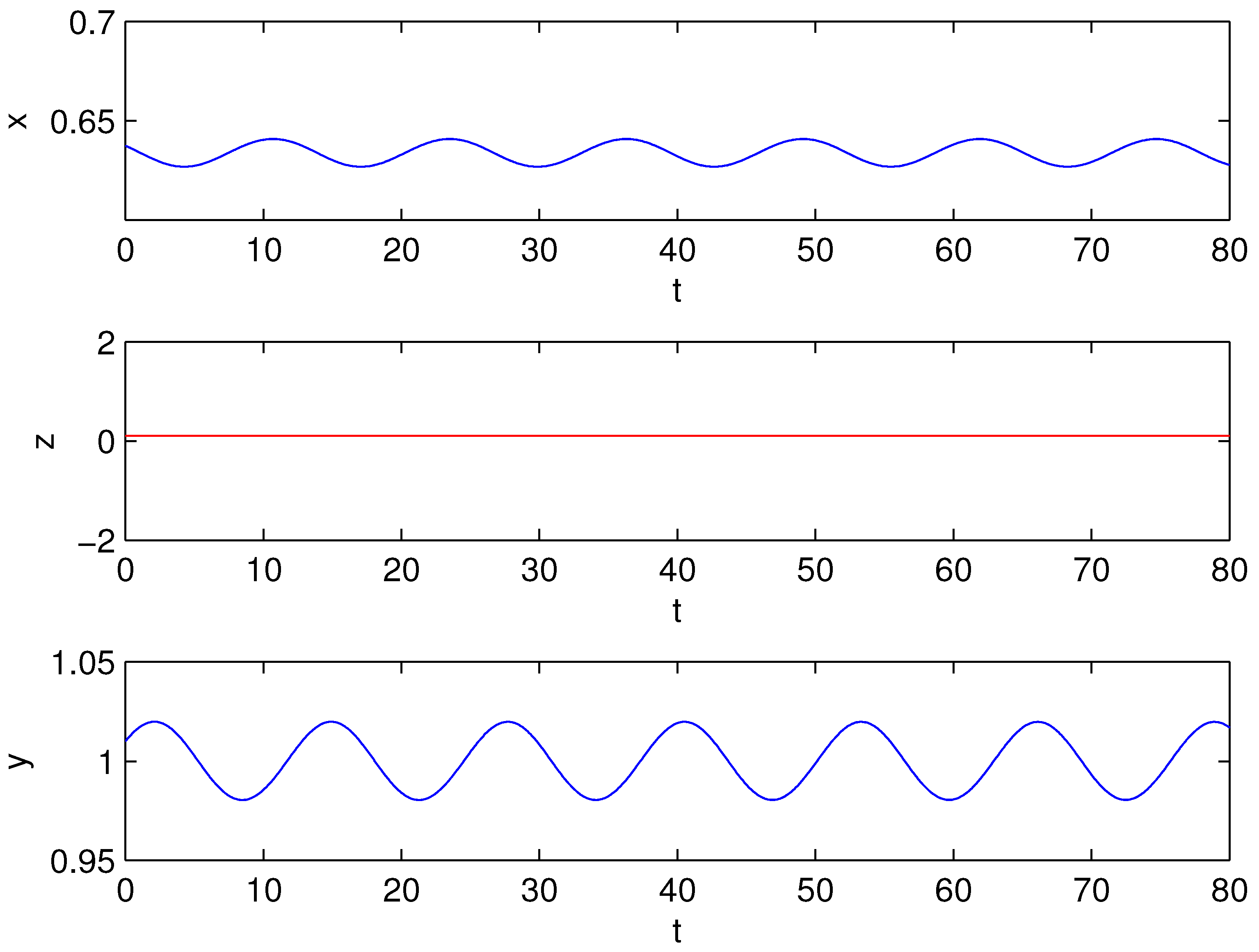
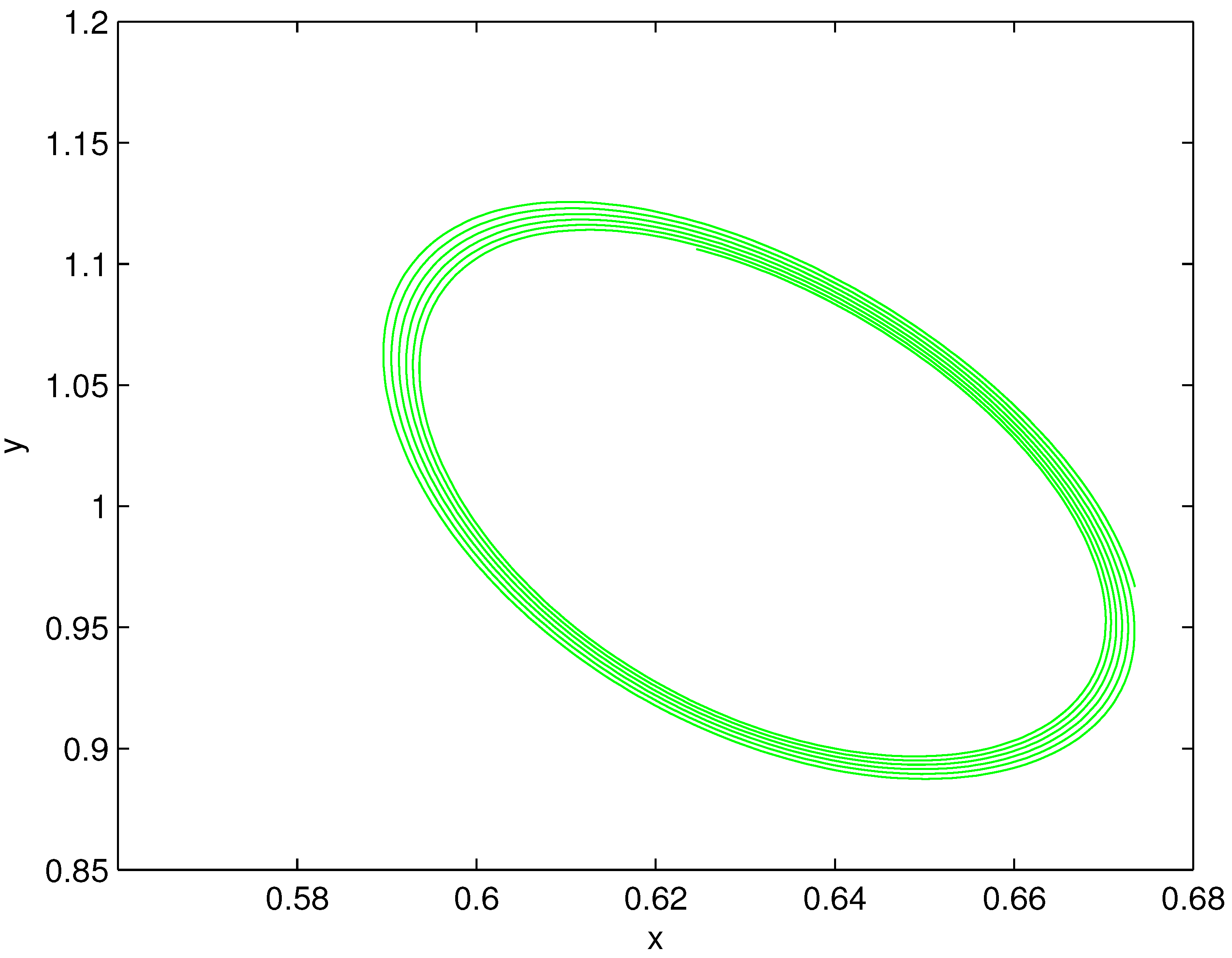
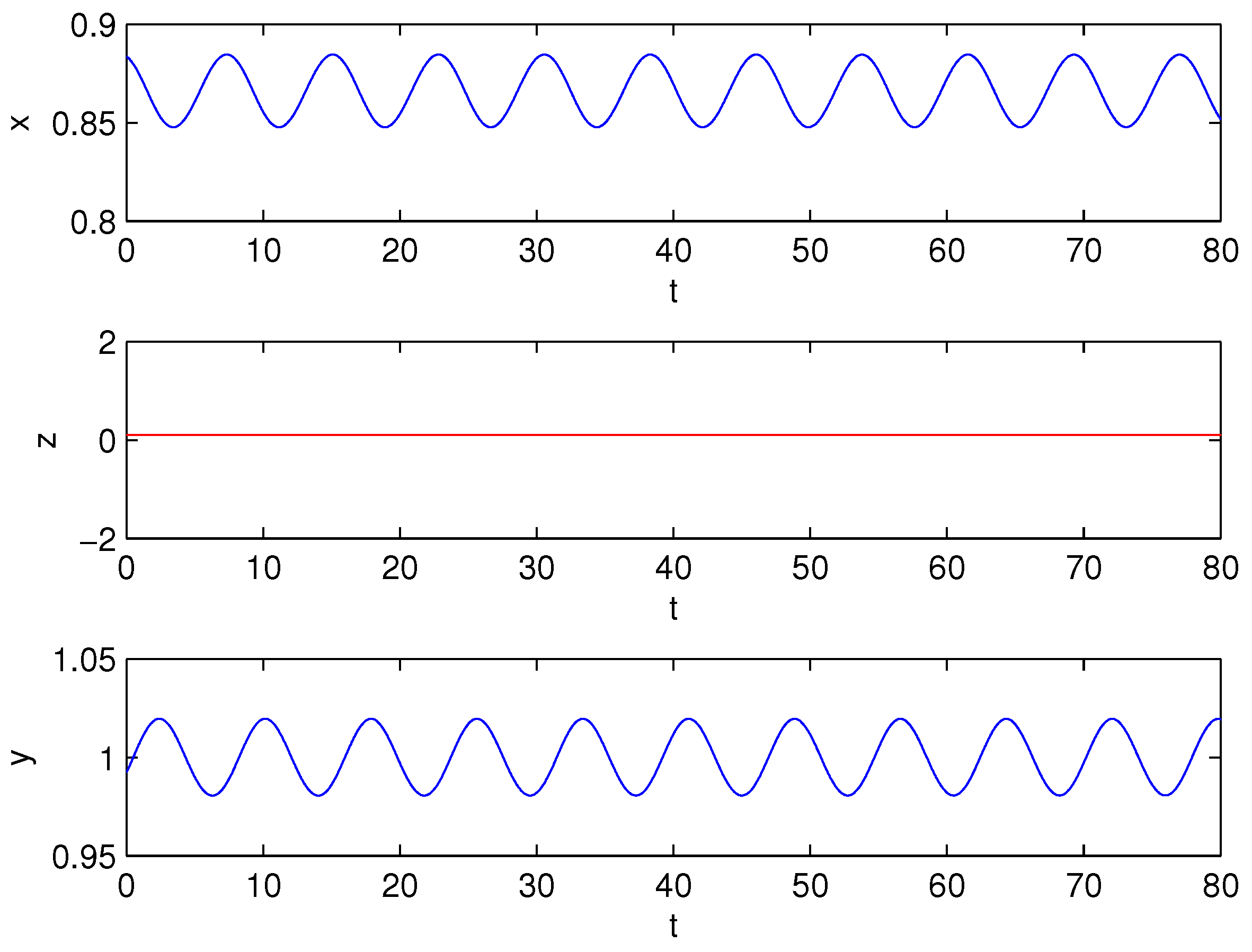
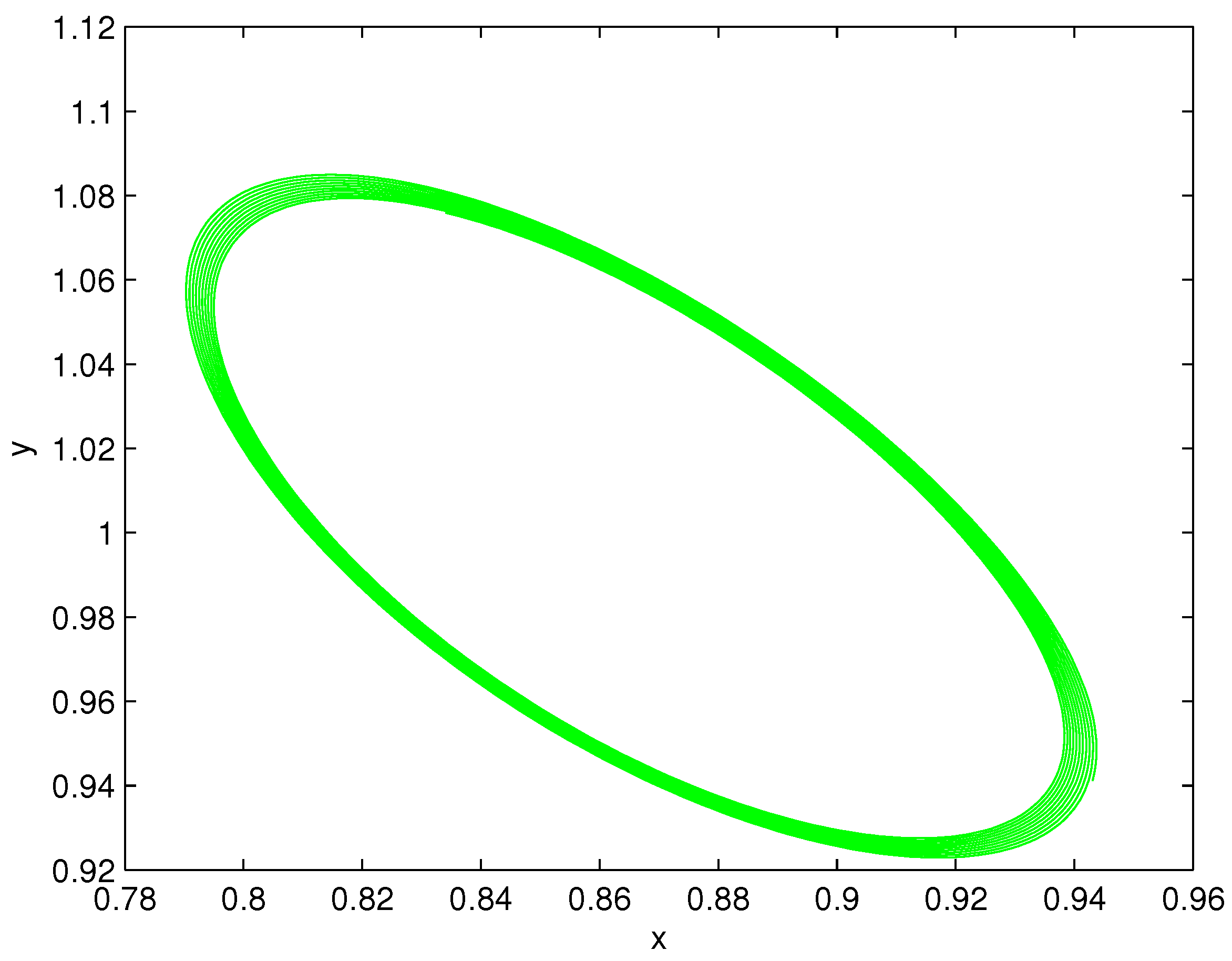
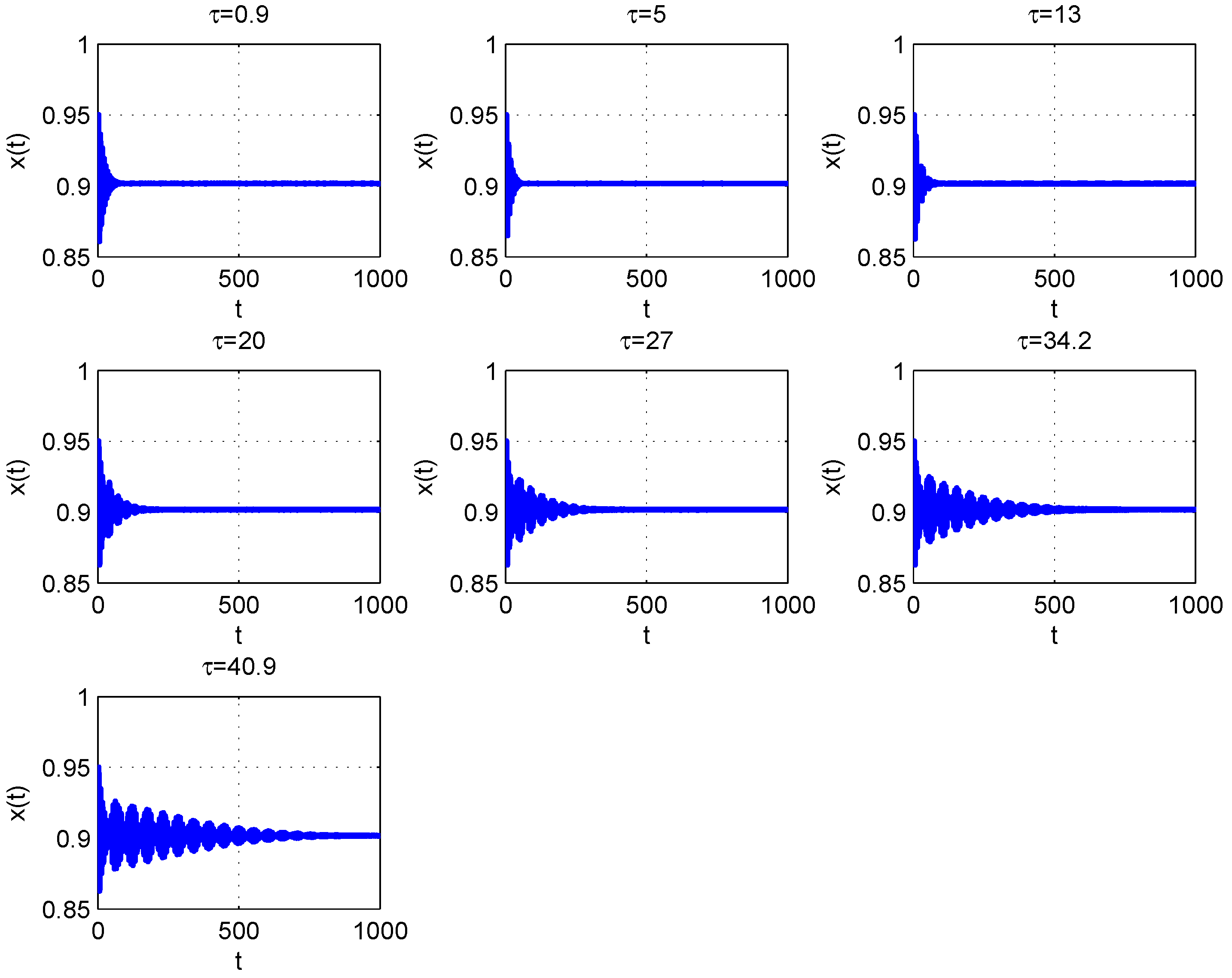
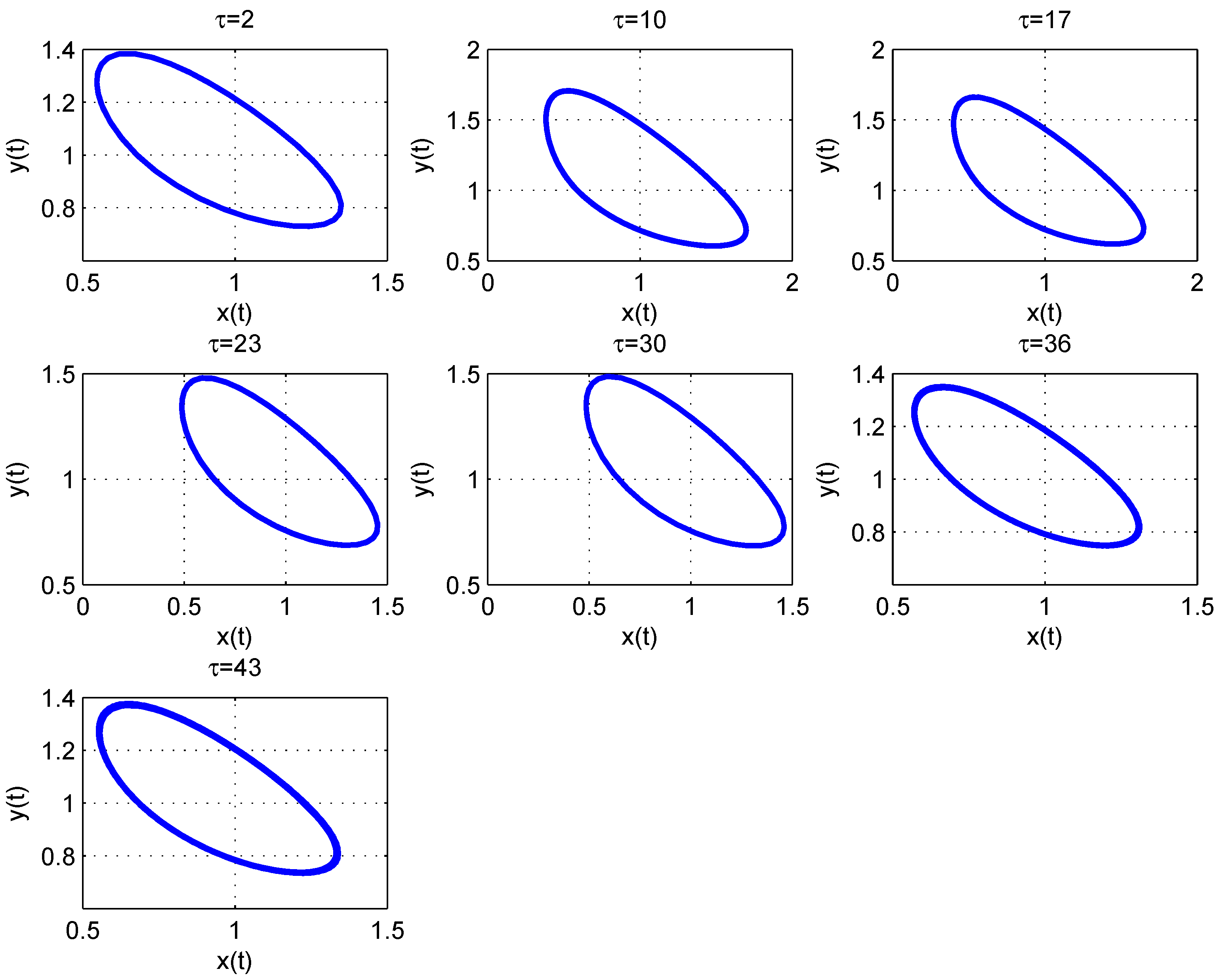
and otherwise it is unstable. Moreover, the Hopf bifurcation occurs when and for As discussed in Section 4.2, for we find that and . Thus, we get and , hence, the system undergoes supercritical Hopf bifurcation at the equilibrium and the bifurcating periodic solution is stable. As seen in Figure 10, delayed model (14) approaches stable fixed points for for for example and Moreover, the delayed model (14) has periodic solution when for as shown in Figure 11.
5. Discussion
As compared to the marketing strategies, advertising has striking advantages, for instance, the cost of it is significantly lower and its propagation is much faster especially on social media. It is supposed that the product information disseminates thanks to twice ways: word-of-mouth among people’s direct contacts and advertising. We investigated the effect of advertising diffusion to convert potential buyers into actual customers in order reveal the frequent fluctuations in sales and advertising over time. For the sake of completion the study, we must not lose sight of the period of influence of advertisements on individuals. It is expected that it will be encountered by a time delay in the duration of the effect. Therefore, model has been divided into continuous and delayed versions to analyze the dynamic behavior extensively.
In order to analyze the dynamics of system it is noted that system (3) has two kinds of equilibria, semi-trivial and nontrivial equilibria which exist for all values of parameters. The local stability behavior was carried out of the system around each equilibria for both delayed (15) and non-delayed (3) systems. According to the concepts of theory of Hopf bifurcation, the continuous system undergoes supercritical Hopf bifurcation under specific conditions, and the formula for critical value of the bifurcation parameter was derived. However, this result illustrates that advertising has a periodic effect on the consumers. Therefore, businesses deem the investment tradeoff between advertising and product services, rationally optimizes resource allocation from service level, product quality, creative advertising, packaging design, etc., to ameliorate its market share and maximize their enterprize profits.
Author Contributions
Software and Writing—original draft, M.A.A.-R. and M.Z.; Writing—review and editing, S.A. and C.C. All authors have read and agreed to the published version of the manuscript.
Funding
The authors extend their appreciation to the Deanship of Scientific Research at King Khalid University for funding this work through Research Group Program under grant number RGP. 1/58/42.
Data Availability Statement
No data were used to support this study.
Acknowledgments
The authors extend their appreciation to the Deanship of Scientific Research at King Khalid University for funding this work through Research Group Program under grant number RGP. 1/58/42. Furthermore, the authors would like to thank Jingli Ren for valuable suggestions incorporated into this work, which actively contributed to refining of the study.
Conflicts of Interest
The authors declare no conflict of interest.
References
- Smith, R.E.; Chen, J.; Yang, X. The impact of advertising creativity on the hierarchy of effects. J. Advert. 2008, 37, 47–62. [Google Scholar] [CrossRef]
- Blecher, E. The impact of tobacco advertising bans on consumption in developing countries. J. Health Econ. 2008, 27, 930–942. [Google Scholar] [CrossRef]
- Aslam, S.; Jadoon, E.; Zaman, K.; Gondal, S. Effect of word of mouth on consumer buying behavior. Mediterr. J. Soc. Sci. 2011, 2, 497. [Google Scholar]
- He, Q.; Qu, H. The impact of advertising appeals on purchase intention in social media environment analysis of intermediary effect based on brand attitude. J. Bus. Adm. Res. 2018, 7, 17. [Google Scholar] [CrossRef] [Green Version]
- Jovanović, P.; Vlastelica, T.; Kostić, S.C. Impact of advertising appeals on purchase intention. Manag. J. Sustain. Bus. Manag. Solut. Emerg. Econ. 2017, 21, 35–45. [Google Scholar]
- Bass, F.M. A new product growth model for consumer durables. Manag. Sci. 1969, 15, 215–322. [Google Scholar] [CrossRef]
- Dodson, J.A., Jr.; Muller, E. Models of new product diffusion through advertising and word-of-mouth. Manag. Sci. 1978, 24, 1568–1578. [Google Scholar] [CrossRef] [Green Version]
- Feichtinger, G. Hopf bifurcation in an advertising diffusion model. J. Econ. Behav. Organ. 1992, 17, 401–411. [Google Scholar] [CrossRef]
- Landa, F.J.; Velasco, F. Dynamic analysis of the current market and potential of organizations. Eur. J. Manag. Econ. Co. 2004, 13, 131–140. [Google Scholar]
- Nie, P.; Abd-Rabo, M.A.; Sun, Y.; Ren, J. A consumption behavior model with advertising and word-of-mouth effect. J. Nonlinear Model. Anal. 2019, 1, 461–489. [Google Scholar]
- Feichtinger, G.; GHEZZI, L.L.; Piccardi, C. Chaotic behavior in an advertising diffusion model. Int. J. Bifurc. Chaos 1995, 5, 255–263. [Google Scholar] [CrossRef]
- Sirghi, N.; Neamtu, M. Deterministic and stochastic advertising diffusion model with delay. WSEAS Trans. Syst. Control 2013, 4, 141–150. [Google Scholar]
- Kuznetsov, Y.A. Elements of Applied Bifurcation Theory, 2nd ed.; Marsden, J.E., Sirovich, L., Eds.; Springer: New York, NY, USA, 1998. [Google Scholar]
- Ren, J.; Yuan, Q. Bifurcations of a periodically forced microbial continuous culture model with restrained growth rate. Chaos Interdiscip. J. Nonlinear Sci. 2017, 27, 083124. [Google Scholar] [CrossRef] [PubMed] [Green Version]
- Ren, J.; Yu, L.; Zhu, H. Dynamic analysis of discrete-time, continuous-time and delayed feedback jerky equations. Nonlinear Dyn. 2016, 86, 107–130. [Google Scholar] [CrossRef]
- Charykov, N.A.; Charykova, M.V.; Semenov, K.N.; Keskinov, V.A.; Kurilenko, A.V.; Shaimardanov, Z.K.; Shaimardanova, B.K. Multiphase open phase processes differential equations. Processes 2019, 7, 148. [Google Scholar] [CrossRef] [Green Version]
- Li, H.; Cheng, J.; Li, H.B.; Zhong, S.-M. Stability analysis of a fractional-order linear system described by the caputo–fabrizio derivative. Mathematics 2019, 7, 200. [Google Scholar] [CrossRef] [Green Version]
- Mahmoud, G.M.; Arafa, A.A.; Mahmoud, E.E. Bifurcations and chaos of time delayed Lorenz system with dimension 2n + 1. Eur. Phys. J. Plus 2017, 132, 461. [Google Scholar] [CrossRef]
- Li, L.; Shen, J. Bifurcations and dynamics of the Rb-E2F pathway involving miR449. Complexity 2017, 2017, 1409865. [Google Scholar] [CrossRef] [Green Version]
- Rihana, F.A.; Lakshmananb, S.; Maurer, H. Optimal control of tumour-immune model with time-delay and immuno-chemotherapy. Appl. Math. Comput. 2019, 353, 147–165. [Google Scholar] [CrossRef]
- Yin, Z.; Yu, Y.; Lu, Z. Stability analysis of an age-structured SEIRS model with time delay. Mathematics 2020, 8, 455. [Google Scholar] [CrossRef] [Green Version]
- Sun, C.; Lin, Y.; Han, M. Stability and Hopf bifurcation for an epidemic disease model with delay. Chaos Solitons Fractals 2006, 30, 204–216. [Google Scholar] [CrossRef]
- Wang, F.; Wang, H.; Xu, K. Diffusive logistic model towards predicting information diffusion in online social networks. In Proceedings of the 2012 32nd International Conference on Distributed Computing Systems Workshops, Macau, China, 18–21 June 2012; pp. 133–139. [Google Scholar]
- J<i>a</i>¨ntschi, L. The eigenproblem translated for alignment of molecules. Symmetry 2019, 11, 1027. [Google Scholar] [CrossRef] [Green Version]
- Dimitrova, N.; Zlateva, P. Global stability analysis of a bioreactor model for phenol and Cresol Mixture Degradation. Processes 2021, 9, 124. [Google Scholar] [CrossRef]
- Hassard, B.D.; Kazarinoff, N.D.; Wan, Y.W. Theory and Applications of Hopf Bifurcation; Cambridge University Press: Cambridge, UK, 1981; Volume 41. [Google Scholar]
- Song, Y.; Wei, J. Bifurcation analysis for Chen’s system with delayed feedback and its application to control of chaos. Chaos Solitons Fractals 2004, 22, 75–91. [Google Scholar] [CrossRef]
- Yang, J.; Zhao, L. Bifurcation analysis and chaos control of the modified Chua’s circuit system. Chaos Solitons Fractals 2015, 77, 332–339. [Google Scholar] [CrossRef]
Figure 1.
Hopf bifurcation Diagrams of model at (3) for bifurcation values of .
Figure 1.
Hopf bifurcation Diagrams of model at (3) for bifurcation values of .

Figure 2.
Hopf bifurcation Diagrams of model at (3) for bifurcation values of .
Figure 2.
Hopf bifurcation Diagrams of model at (3) for bifurcation values of .

Figure 3.
The time series at , .

Figure 4.
The phase portrait of the limit cycle at , .

Figure 5.
The time series at ,

Figure 6.
The phase portrait of the limit cycle at , .

Figure 7.
The time series at , .

Figure 8.
The phase portrait of the limit cycle at , .

Figure 9.
The critical time delays (blue curves) and (red dash curves) for system (14) against .
Figure 9.
The critical time delays (blue curves) and (red dash curves) for system (14) against .

Figure 10.
The stable solution of system (14) with different values of .
Figure 10.
The stable solution of system (14) with different values of .

Figure 11.
Periodic solutions of system (14) with different values of .
Figure 11.
Periodic solutions of system (14) with different values of .


Table 1.
The meaning of the coefficients in the system.
| The Symbol | The Meaning |
|---|---|
| individuals stream into the firms market, | |
| the current customers leaving the market forever, | |
| current customers switching to a rival brand, | |
| proportionality measuring of the advertising effectiveness. |
Publisher’s Note: MDPI stays neutral with regard to jurisdictional claims in published maps and institutional affiliations. |
© 2021 by the authors. Licensee MDPI, Basel, Switzerland. This article is an open access article distributed under the terms and conditions of the Creative Commons Attribution (CC BY) license (http://creativecommons.org/licenses/by/4.0/).
Share and Cite
MDPI and ACS Style
Abd-Rabo, M.A.; Zakarya, M.; Cesarano, C.; Aly, S. Bifurcation Analysis of Time-Delay Model of Consumer with the Advertising Effect. Symmetry 2021, 13, 417. https://0-doi-org.brum.beds.ac.uk/10.3390/sym13030417
AMA Style
Abd-Rabo MA, Zakarya M, Cesarano C, Aly S. Bifurcation Analysis of Time-Delay Model of Consumer with the Advertising Effect. Symmetry. 2021; 13(3):417. https://0-doi-org.brum.beds.ac.uk/10.3390/sym13030417
Chicago/Turabian StyleAbd-Rabo, Mahmoud A., Mohammed Zakarya, Clemente Cesarano, and Shaban Aly. 2021. "Bifurcation Analysis of Time-Delay Model of Consumer with the Advertising Effect" Symmetry 13, no. 3: 417. https://0-doi-org.brum.beds.ac.uk/10.3390/sym13030417
Note that from the first issue of 2016, this journal uses article numbers instead of page numbers. See further details here.