A Novel Neural Network Training Algorithm for the Identification of Nonlinear Static Systems: Artificial Bee Colony Algorithm Based on Effective Scout Bee Stage

Abstract

In this study, a neural network-based approach is proposed for the identification of nonlinear static systems. A variant called ABCES (ABC Based on Effective Scout Bee Stage) is introduced for neural network training. Two important changes are carried out with ABCES. The first is an update of “limit” control parameters. In ABC algorithm, “limit” value is fixed. It is adaptively adjusted according to number of iterations in ABCES. In this way, the efficiency of the scout bee stage is increased. Secondly, a new solution-generating mechanism for the scout bee stage is proposed. In ABC algorithm, new solutions are created randomly. It is aimed at developing previous solutions in the scout bee stage of ABCES. The performance of ABCES is analyzed on two different problem groups. First, its performance is evaluated on 13 numerical benchmark test problems. The results are compared with ABC, GA, PSO and DE. Next, the neural network is trained by ABCES to identify nonlinear static systems. 6 nonlinear static test problems are used. The performance of ABCES in neural network training is compared with ABC, PSO and HS. The results show that ABCES is generally effective in the identification of nonlinear static systems based on neural networks.

1. Introduction

One of the most important issues of artificial intelligence is heuristic optimization algorithms. They are used to solve many real-world problems and provide many advantages. Therefore, the number of heuristic optimization algorithms has increased recently. Heuristic optimization algorithms are divided into different classes according to the source of inspiration such as swarm intelligence, bio-inspired, physics and chemistry-based, and other algorithms [1]. ABC algorithm is one of the most popular heuristic algorithms based on swarm intelligence. It is used to solve many problems in different areas.

One of the other important usage areas of ABC algorithm is artificial neural network (ANN) training. ANN produces output values by using input values. It can learn with samples. The learning process continues according to a tolerance value. The information obtained as a result of learning is stored in weights. In this way, using weights can produce suitable results in the face of similar situations. This is a very important advantage of ANN. It is one of the main reasons for choosing ANN within the scope of this study.

In our daily life, we encounter nonlinear systems in all areas. Some exhibit static, others dynamic behavior. In fact, this is why the identification of nonlinear systems is important. When the literature is examined, studies have been carried out on nonlinear dynamic systems generally in system identification. In other words, nonlinear static systems are ignored. Nonlinear dynamic systems are affected by previous times. Time series is one of the most important examples of these systems. Nonlinear static systems are time independent. They are formed as a result of the interaction of independent variables. In fact, many fields such as education, medicine, engineering, finance, business exhibit static behavior. This is the main difference between nonlinear static and dynamic systems. This structural difference affects the complexity level of the systems. This study focuses directly on the identification of nonlinear static systems.

Neuro-fuzzy and ANN are popular methods used in prediction and modeling. Both methods can learn with samples. The learning process makes the methods powerful. This situation allows the generation of an output for input values that they do not know at all. Although both methods have strengths and weaknesses according to problem types, there is no definite inference. Experiences are decisive in this process. In [2,3,4,5], ANFIS, one of the neuro-fuzzy models, was trained using ABC algorithm for the identification of nonlinear dynamic/static systems. In these studies, the performance of ANFIS training-based ABC algorithm on system identification was observed. However, the performance of ANN training based on ABC algorithm in the identification of nonlinear static systems is unknown. In [6], ANN was trained using the ABC algorithm for pattern classification. But it is not about system identification. Therefore, ANN training is carried out by using ABC algorithm and its variant to identify nonlinear static systems in this study. The performance of approaches such as ABC algorithm, PSO and HS are analyzed comparatively in the identification of nonlinear static systems for the first time. In this respect, it is a pioneering and innovative study. In fact, it is one of the first studies whose main subject is the identification of nonlinear static systems. Within the scope of this study, only standard ABC algorithm is not used for ANN training. A novel algorithm called ABCES based on ABC algorithm is introduced for ANN training. With ABCES, two important changes are realized in structure of ABC algorithm. The first is adjustment of limit control parameter. Unlike standard ABC algorithm, this control parameter is not fixed. It is determined adaptively. The second is updating of solution generation mechanism belonging to the scout bee stage. In standard ABC algorithm, the solutions for the scout bee stage are generated randomly. In the proposed method, a new solution generation mechanism that uses the global best solution to ensure the continuity of the gains achieved, has been proposed. In this way, the scout bee stage has been made more effective. These changes are an innovative approach to improving the performance of standard ABC algorithm.

2. Related Works

2.1. The Studies on ABC Algorithm

Some studies related to ABC algorithm are presented in this section. Horng [7] suggested a max entropy thresholding (MET) approach based on ABC algorithm for image segmentation. The study compared the results obtained with four different methods: PSO, hybrid cooperative-comprehensive learning-based PSO algorithm (HCOCLPSO), Fast Otsu’s method and honey-bee mating optimization (HBMO). Karaboga [8] designed digital infinite impulse response (IIR) filters by using ABC algorithm. Yeh and Hsieh [9] solved reliability redundancy allocation problem by using a variant of ABC algorithm and the results were compared with different methods in the literature. Hemamalini and Simon [10] used ABC algorithm for economic load dispatch problem. Hong [11] proposed a model to predict electric load based on support vector regression (SVR) and ABC algorithm. Şahin [12] used GA and ABC to maximize the thermal performance of a solar air collector. Zaman et al. [13] proposed a method based on ABC algorithm for synthesizing antenna arrays. Deng [14] used ABC algorithm to classify customers in mobile e-commerce environment. Bulut and Tasgetiren [15] developed a variant of ABC algorithm for economic lot scheduling problem. There are many studies related to ABC algorithm out of these [16,17,18].

Although ABC algorithm’s global convergence speed is very good, its different variants have been proposed to increase the speed of local convergence of ABC algorithm. The main purpose here is to improve the performance of ABC algorithm. Bansal et al. [19] proposed adaptive version of ABC algorithm. Here, two important parameters were adjusted according to current fitness values adaptively: step size and “limit” control parameters. Babaeizadeh and Ahmad [20] updated employed, onlooker and scout bee phases in ABC algorithm. Draa and Bouaziz [21] suggested a new ABC algorithm for image contrast enhancement. Karaboga and Gorkemli [22] proposed a variant known as qABC and modified solution generation mechanism belonging to onlooker phase. Gao et al. [23] presented new solution generation mechanisms using more information about the population. Wang [24] made two important updates via generalized opposition-based learning method and local best solution in ABC algorithm. Kıran and Fındık [25] added direction information for each dimension of each food source position to increase the speed of convergence of ABC algorithm. Liang and Lee [26] updated ABC algorithm using different operations and strategies such as elite, solution sharing, instant update, cooperative strategy and population manager strategies. Karaboga and Kaya [4] used arithmetic crossover and adaptive neighborhood radius to improve the performance of ABC algorithm. Different variants of ABC algorithm have been proposed out of these [27,28,29,30].

2.2. The Studies on ANN and Neuro-Fuzzy

Due to advantages of ANN, it is seen that it is used successfully in solving many real-world problems [31,32,33,34,35]. Capizzi et al. [36] proposed neural network topology to model surface plasmon polaritons propagation. Sciuto et al. [37] suggested an approach based on a spiking neural network for anaerobic digestion process. Capizzi et al. [38] used a back-propagation neural network (BPNN) for automated oil spill detection by satellite remote sensing. An effective training algorithm should be used to achieve effective results with ANN. Therefore, heuristic algorithms have been used extensively in ANN training recently. ABC algorithm is one of successful heuristic algorithms and it is used in ANN training. Mohmad Hassim and Ghazali [39] suggested an approach for training functional link neural network (FLNN) by using ABC algorithm for time series prediction. They demonstrated that the proposed approach was better than FLNN model based on BP. Zhang et al. [40] suggested a model based on a forward neural network for classifying MR brain image and adjusted with ABC algorithm the parameters of a forward neural network. Ozkan et al. [41] used a model-based neural network and ABC for modeling daily reference evapotranspiration. Chen et al. [42] used an approach based on BPNN and ABC algorithm for prediction of water quality. Karaboga and Ozturk [6] applied ABC algorithm to train FFNNs on pattern classification. The benchmark classification problems were used for performance analysis. Obtained results by using ABC algorithm was compared with the well-known some algorithms. It was reported that training FFNN based on ABC algorithm gave effective results on the related problem. Another usage area of ABC algorithm is ANFIS training. Karaboga and Kaya [2,3] used standard ABC algorithm for adaptive-network-based fuzzy inference system (ANFIS) training for nonlinear dynamic systems identification. In a different study, Karaboga and Kaya [4] proposed a new ANFIS training algorithm called an adaptive and hybrid artificial bee colony algorithm (aABC) to obtain more effective results in the identification of nonlinear dynamic systems. In the next study, Karaboga and Kaya [5] trained ANFIS by using aABC algorithm for nonlinear static systems identification. The performance of aABC algorithm was tested on 5 nonlinear static systems and compared with PSO, GA, HS and ABC algorithm.

3. Materials and Methods

3.1. Standard ABC Algorithm

The ABC algorithm is one of the popular swarm-based heuristic optimization algorithms. It models the food searching behavior of the honey-bees [43]. It includes three different types of bees named employed bees, onlooker bees and scout bees. There are some assumptions in ABC algorithm. Some of these are: half of the colony consists of employed bees. The other half is the onlooker bees. Specifically, the number of employed bees is equal to the number of onlooker bees. The basic steps of ABC algorithm are as follows:

In the initial phase, the positions of food sources are determined randomly by using (1). Here, $x_i$ shows ith solution. i is in range [1, population size]. $x_j^{min}$ is the lower value to be taken by parameter j. Also, $x_j^{max}$ is the upper value.

$$x_{ij}=x_j^{min}+rand(0,1)\left(x_j^{max}-x_j^{min}\right)$$

(1)

Every employed bee probabilistically develops a new food source using the solution positions in memory. (2) is used to create a new solution in this process. Here, k is an integer number in range [1, number of employed bees]. ${\mathsf{\Theta }}_{ij}$ is a random number in range [−1, 1].

$$v_{ij}=x_{ij}+{\mathsf{\Theta }}_{ij}\left(x_{ij}-x_{kj}\right)$$

(2)

If the amount of nectar of the new source is higher than before, information belonging to the previous position is deleted from the memory. At the same time, information belonging to the new food source is written to the memory. Otherwise, the previous position is maintained. After the search process is completed, the employed bees share the food source information with the onlooker bees. A onlooker bee evaluates the information of all bees. It selects a source according to the probability value obtained from (3). As in the employed bee stage, a new solution develops by modifying the current solution. And they control the nectar quantity of the candidate solution. If the nectar amount of the candidate solution is better, information of the previous solution is deleted from the memory.

$$p_i=\frac{fi{t}_i}{{\sum }_1^{SN}fi{t}_n}$$

(3)

“Limit” is one of the important control parameters of ABC algorithm. If a position is not improved up to the limit value, it is assumed that this food source was abandoned. The abandoned food source is replaced by a new food source by scout bee.

3.2. Artificial Bee Colony Algorithm Based on Effective Scout Bee (ABCES)

One of the most important control parameters of ABC algorithm is “limit”. Failure counter is the number of failures in producing the solution. When the failure counter reaches “limit” value, a random solution is created instead of the previous solution. This prevents the creation of qualified solutions. In the scout bee phase, instead of creating solutions randomly, it is aimed to be transformed into more qualified individuals. In this study, two major changes have been made in the structure of standard ABC algorithm. The main purpose of these changes is to make the scout bee stage more effective. With this modification, the convergence speed and solution quality of the algorithm are improved.

To make the scout bee stage more efficient, a strategy has been proposed to determine the limit control parameter. In the standard ABC algorithm, limit value is fixed throughout all iterations. This causes to go the scout bee stage less frequently to produce a new solution. limit value is adaptively determined by using (4) to prevent this.

$$limit=1+w\times D\times FoodNumber\times \left(\right(maxCycle-iter)/maxCycle)$$

(4)

Here, the maximum value of limit value is 1 + D × FoodNumber. maxCycle is the maximum number of iterations, and iter represents the number of current iterations. The limit value is adaptively adjusted according to the number of iterations. Initially, (maxCycle−iter)/maxCycle gets the maximum value and limit has the greatest value in the same way. In fact, the maximum value of limit is adaptively adjusted here. At each iteration, limit value changes. limit is set according to the value of w. w is a random number in the range [0, 1]. It is ensured that the value of the limit is within the range [1, $Uppe{r}_{limit}$]. $Uppe{r}_{limit}$ is found by using (5).

$$Uppe{r}_{limit}=1+D\times FoodNumber\times ((maxCycle-iter)/maxCycle)$$

(5)

The scout bee stage becomes more effective with the change in limit. In this case, an effective solution-generating mechanism is needed to obtain more qualified solutions. The main purpose here is to continue with a more effective solution than the previous solution. Therefore, the solution-generating mechanism given in (6) is proposed.

$$v_{ij}=\left\{\begin{array}{cc}{x}_{ij}\gamma +x_j^g(1-\gamma ),& r1<r2\\ x_{ij}+x_{ij}\times \delta ,& \mathrm{other}\end{array}\right.$$

(6)

$$r2=rand+\left(\right(maxCycle-iter)/maxCycle)$$

(7)

Here, $x^g$ is the global best solution. r1 is a random number in the range [0, 1]. r2 is determined by (7). $\gamma$ is the arithmetic crossover rate and is calculated randomly. $\delta$ is the step size and is accepted as 0.01. Arithmetic crossover is applied between the current solution and the global best solution. In other words, the quality of the current solution is being improved by approximating the global best solution. The value of r2 is randomly generated depending on the number of iterations. Thus, the related solution closes global best solution at first. In this way, the local convergence speed of the algorithm increases. Three different preventions are taken to prevent locally minimal risk. First, the arithmetic crossover rate is randomly selected. Secondly, when not r1 < r2, a new solution is produced in the neighborhood of the current solution. This is achieved via the step size ($\delta$). In particular, in high iterations, outside of global best solution, new solutions are produced according to the current solution. Therefore, quality solutions can even be obtained in high iterations. The third is the possibility of updating the current and global best solution in employed and onlooker bee stages. At the same time, it has been ensured that the new solutions are different from the global best solution with three different preventions.

In summary, adaptive adjustment of limit value is provided. The effectiveness of the scout bee stage is increased with new limit calculation method. A new solution-generating mechanism is proposed for the scout bee stage. In this way, the local convergence speed of the algorithm is increased, and it is provided that better quality solutions are obtained.

3.3. Training Feed Forward Artificial Neural Networks

Artificial neural Networks (ANNs) are one of the artificial intelligence techniques. ANNs consist of the interconnection of artificial neurons. Figure 1 shows the general structure of an artificial neuron. An artificial neuron consists of inputs, weights, bias value, activation and transfer function. In this way, an output is obtained from the inputs of neurons. The output of a neuron is calculated using (8). x is the input value. w are the weight values corresponding to the input. b is bias value. f is the activation function. y corresponds to the output of the artificial neuron.

$$y=f\left(\sum _{i=1}^m{w}_i{x}_i+b\right)$$

(8)

A FFNN consists of 3 layers as input, hidden and output. In FFNN, calculations specified in (8) are performed in each neuron. In this way, each neuron affects the neurons in the next layer. There is no interaction in the same layer. In FFNN, output is obtained corresponding to the input values. This is only possible by creating a model for a related problem. For this, the network needs to be trained. Training the network is the process of determining the weights and bias values. Training algorithms are used for this. One of the learning methods is learning with samples. Training dataset is required for this. It reflects the characteristics of the network and the network learns in the training process. The learning level of the network is related to the error value. Error value refers to the relationship between the real output and predicted output. A low error value is very important for a successful training process. For low error value, an effective training algorithm is required.

4. Simulation Results

4.1. Solution of Global Optimization Problems

In applications, 13 numerical test problems are used to analyze the performance of ABCES algorithm. The related problems are given in

Table 1. Benchmark functions used in experiments.

Function	Formulation
SumSquares	$f\left(x\right)={\sum }_{i=1}^{n}i{x}_i^2$
Levy	$f\left(x\right)={sin}^2\left(\pi w_1\right)+{\sum }_{i=1}^{n-1}{(w_i-1)}^2[1+10{sin}^2(\pi w_i+1)]+{(w_d-1)}^2+[1+{sin}^2\left(2\pi w_d\right)]$ $w_i=1+\frac{x_i-1}{4}$
Rosenbrock	$f\left(x\right)={\sum }_{i=1}^{n-1}[100{(x_{i+1}-x_i^2)}^2+{(x_i-1)}^2]$
The Sum of Different Powers	$f\left(x\right)={\sum }_{i=1}^n{\left|x_i\right|}^{i+1}$
Zakharov	$f\left(x\right)={\sum }_{i=1}^n{x}_i^2+{\left({\sum }_{i=1}^{n}0.5i{x}_i\right)}^2+{\left({\sum }_{i=1}^{n}0.5i{x}_i\right)}^4$
Ackley	$f\left(x\right)=-20exp\left(-0.2\sqrt{\frac{1}{n}{\sum }_{i=1}^n{x}_i^2}\right)-exp\left(\frac{1}{n}{\sum }_{i=1}^{n}cos\left(2\pi x_i\right)\right)+20+e$
Step	$f\left(x\right)={\sum }_{i=1}^n{\left(⌊x_i+0.5⌋\right)}^2$
Rastrigin	$f\left(x\right)={\sum }_{i=1}^n\left[x_i^2-10cos\left(2\pi x_i\right)+10\right]$
Griewank	$f\left(x\right)=\frac{1}{4000}{\sum }_{i=1}^n{x}_i^2+{\prod }_{i=1}^{n}cos\left(\frac{x_i}{\sqrt{i}}\right)+1$
Rotated Hyper-Ellipsoid	$f\left(x\right)={\sum }_{i=1}^n{\sum }_{j=1}^i{x}_j^2$
Dixon–Price	$f\left(x\right)={(x_1-1)}^2+{\sum }_{i=2}^{n}i{(2x_i^2-x_{i-1})}^2$
Perm	$f\left(x\right)={\sum }_{k=1}^n{\left[{\sum }_{i=1}^n(i^k+\beta )\left({\left(\frac{x_i}{i}\right)}^k-1\right)\right]}^2$
Sphere	$f\left(x\right)={\sum }_{i=1}^n{x}_i^2$

. For ABC and ABCES algorithms, population size is taken as 50. The results are obtained for different values of D ∈ {50,100,150,1000}. The number of evaluations has been used 100,000, 500,000, 1,000,000 values. Each application is run 30 times. Each initial population is determined randomly.

The results found with ABC and ABCES algorithms in 100,000 evaluations are given in

Table 2. Comparison of the results obtained by using ABC and ABCES (D: Dimension, Mean: Mean Values, SD: Standard Deviation, Population Size = 50, Number of Evaluation = 100,000.)

No	Function	Range	D	ABC		ABCES (Proposed)
				Mean	SD	Mean	SD
1	SumSquares	[−10, 10]	50	$9.61\times {10}^{-10}$	$1.94\times {10}^{-9}$	$2.25\times {10}^{-14}$	$2.65\times {10}^{-14}$
			100	$7.87\times {10}^{-3}$	$3.96\times {10}^{-2}$	$4.75\times {10}^{-6}$	$4.74\times {10}^{-6}$
			150	$9.90\times {10}^{-1}$	2.60	$5.80\times {10}^{-4}$	$4.62\times {10}^{-4}$
2	Levy	[−10, 10]	50	$1.28\times {10}^{-10}$	$3.66\times {10}^{-10}$	$7.69\times {10}^{-11}$	$1.29\times {10}^{-10}$
			100	$4.97\times {10}^{-4}$	$1.26\times {10}^{-3}$	$1.63\times {10}^{-5}$	$1.55\times {10}^{-5}$
			150	$1.57\times {10}^{-2}$	$3.82\times {10}^{-2}$	$1.15\times {10}^{-3}$	$8.41\times {10}^{-4}$
3	Sphere	[−100, 100]	50	$3.21\times {10}^{-9}$	$7.92\times {10}^{-9}$	$1.05\times {10}^{-13}$	$1.10\times {10}^{-13}$
			100	$3.53\times {10}^{-2}$	$6.87\times {10}^{-2}$	$5.71\times {10}^{-6}$	$4.65\times {10}^{-6}$
			150	$7.24\times {10}^{-1}$	2.19	$9.15\times {10}^{-4}$	$1.10\times {10}^{-3}$
4	Rosenbrock	[−30, 30]	50	4.55	5.63	2.33	2.70
			100	$2.10\times {10}^2$	$1.16\times {10}^2$	$1.45\times {10}^2$	$6.80\times {10}^1$
			150	$6.69\times {10}^2$	$4.65\times {10}^2$	$4.63\times {10}^2$	$3.54\times {10}^2$
5	The Sum of Different Powers	[−1, 1]	50	$4.48\times {10}^{-17}$	$1.92\times {10}^{-17}$	$2.65\times {10}^{-18}$	$2.24\times {10}^{-18}$
			100	$3.34\times {10}^{-11}$	$1.16\times {10}^{-10}$	$1.06\times {10}^{-15}$	$1.50\times {10}^{-15}$
			150	$1.98\times {10}^{-7}$	$7.54\times {10}^{-7}$	$1.83\times {10}^{-11}$	$4.07\times {10}^{-11}$
6	Zakharov	[−10, 10]	50	$1.12\times {10}^3$	$9.81\times {10}^1$	$1.35\times {10}^2$	$3.16\times {10}^1$
			100	$2.63\times {10}^3$	$1.32\times {10}^2$	$3.50\times {10}^2$	$5.97\times {10}^1$
			150	$4.31\times {10}^3$	$1.78\times {10}^2$	$5.83\times {10}^2$	$1.28\times {10}^2$
7	Ackley	[−32, 32]	50	$3.06\times {10}^{-5}$	$4.98\times {10}^{-5}$	$8.56\times {10}^{-7}$	$3.71\times {10}^{-7}$
			100	$2.46\times {10}^{-1}$	$3.39\times {10}^{-1}$	$2.70\times {10}^{-2}$	$1.94\times {10}^{-2}$
			150	2.01	$4.99\times {10}^{-1}$	1.25	$3.40\times {10}^{-1}$
8	Step	[−100, 100]	50	$6.03\times {10}^{-9}$	$1.82\times {10}^{-8}$	$2.35\times {10}^{-9}$	$4.55\times {10}^{-9}$
			100	$2.80\times {10}^{-2}$	$7.90\times {10}^{-2}$	$1.37\times {10}^{-4}$	$9.29\times {10}^{-5}$
			150	$8.46\times {10}^{-1}$	2.30	$4.25\times {10}^{-3}$	$2.10\times {10}^{-3}$
9	Rastrigin	[−5.12, 5.12]	50	$7.89\times {10}^{-2}$	$2.54\times {10}^{-1}$	$1.89\times {10}^{-1}$	$4.85\times {10}^{-1}$
			100	$1.44\times {10}^1$	4.76	$1.67\times {10}^1$	4.30
			150	$5.57\times {10}^1$	7.85	$6.60\times {10}^1$	7.93
10	Griewank	[−600, 600]	50	$2.54\times {10}^{-5}$	$1.00\times {10}^{-4}$	$3.86\times {10}^{-11}$	$9.49\times {10}^{-11}$
			100	$3.43\times {10}^{-2}$	$5.47\times {10}^{-2}$	$2.84\times {10}^{-3}$	$5.73\times {10}^{-3}$
			150	$2.65\times {10}^{-1}$	$3.14\times {10}^{-1}$	$4.39\times {10}^{-2}$	$3.95\times {10}^{-2}$
11	Rotated Hyper-Ellipsoid	[−65,536, 65,536]	50	$2.03\times {10}^{-4}$	$8.46\times {10}^{-4}$	$2.15\times {10}^{-7}$	$3.50\times {10}^{-7}$
			100	$4.73\times {10}^5$	$1.89\times {10}^6$	6.54	5.38
			150	$2.81\times {10}^7$	$8.16\times {10}^7$	$2.16\times {10}^4$	$2.54\times {10}^4$
12	Dixon–Price	[−10, 10]	50	$4.71\times {10}^{-2}$	$1.20\times {10}^{-1}$	$4.51\times {10}^{-2}$	$2.53\times {10}^{-2}$
			100	$2.42\times {10}^1$	$1.43\times {10}^1$	$1.48\times {10}^1$	8.03
			150	$7.48\times {10}^1$	$3.42\times {10}^1$	$5.92\times {10}^1$	$1.68\times {10}^1$
13	Perm	[−4, 4]	2	$2.54\times {10}^{-9}$	$5.40\times {10}^{-9}$	$5.50\times {10}^{-12}$	$1.41\times {10}^{-11}$
			4	$1.42\times {10}^{-1}$	$1.01\times {10}^{-1}$	$9.35\times {10}^{-3}$	$2.71\times {10}^{-2}$
			6	$2.01\times {10}^3$	$4.18\times {10}^3$	$1.51\times {10}^1$	$2.20\times {10}^1$

. 13 test functions are used, and the results are obtained for D = {50, 100, 150} in each function. In addition to the objective function and standard deviation values are given here. When D is 50, 100 and 150, ABCES algorithm has better results than ABC algorithm in SumSquares, Levy, Sphere, Rosenbrock, The Sum of Different Powers, Zakharov, Ackley, Step, Griewank, Rotated Hyper-Ellipsoid, Dixon–Price and Perm. ABC algorithm is only successful in Rastrigin. Apart from average objective function value, ABCES algorithm is more successful in the standard deviation values. This shows that the results obtained by using ABCES in 100,000 evaluations are more robust. The Wilcoxon signed rank test is used to determine the significance of the results and it is given in

Table 3. Wilcoxon signed rank test results between standard ABC and ABCES (Population Size = 50, Number of Evaluation = 100,000).

No	Function	Range	D	Statistical Results
				p-Value	Significance
1	SumSquares	[−10, 10]	50	0.000	+
			100	0.000	+
			150	0.000	+
2	Levy	[-10, 10]	50	0.041	+
			100	0.002	+
			150	0.165	-
3	Sphere	[−100, 100]	50	0.000	+
			100	0.000	+
			150	0.000	+
4	Rosenbrock	[−30, 30]	50	0.021	+
			100	0.019	+
			150	0.019	+
5	The Sum of Different Powers	[−1, 1]	50	0.000	+
			100	0.000	+
			150	0.000	+
6	Zakharov	[−10, 10]	50	0.000	+
			100	0.000	+
			150	0.000	+
7	Ackley	[−32, 32]	50	0.000	+
			100	0.000	+
			150	0.000	+
8	Step	[−100, 100]	50	0.090	-
			100	0.043	+
			150	0.003	+
9	Rastrigin	[−5.12, 5.12]	50	0.192	-
			100	0.131	-
			150	0.000	*
10	Griewank	[−600, 600]	50	0.000	+
			100	0.000	+
			150	0.000	+
11	Rotated Hyper-Ellipsoid	[−65,536, 65,536]	50	0.000	+
			100	0.000	+
			150	0.000	+
12	Dixon–Price	[−10, 10]	50	0.006	+
			100	0.002	+
			150	0.024	+
13	Perm	[−4, 4]	2	0.000	+
			4	0.000	+
			6	0.000	+

. The evaluation is made according to p = 0.05 level. 13 test functions are evaluated in 3 different dimensions (D = 50, 100, 150). Specifically, the significance of 39 results is examined. A significant difference is found in favor of the ABCES algorithm in 34 of these. This result indicates that ABCES algorithm is better in 34 objective function value. There is no significant difference in 4 results. In only one result, there is significant difference indicating that ABC algorithm is more good.

When the results are obtained in 100,000 evaluations are examined, it is seen that fast convergence continues in the problems. Therefore, it is determined that better results can be achieved in high iteration. Thus, the results found in 500,000 evaluations are given in

Table 4. Comparison of the results obtained by using ABC and ABCES (D: Dimension, Mean: Mean Values, SD: Standard Deviation, Population Size = 50, Number of Evaluation = 500,000).

No	Function	Range	D	ABC		ABCES (Proposed)
				Mean	SD	Mean	SD
1	SumSquares	[−10, 10]	50	$8.81\times {10}^{-16}$	$9.93\times {10}^{-17}$	$1.63\times {10}^{-16}$	$3.20\times {10}^{-17}$
			100	$2.12\times {10}^{-15}$	$1.96\times {10}^{-16}$	$4.08\times {10}^{-16}$	$5.96\times {10}^{-17}$
			150	$3.72\times {10}^{-15}$	$3.94\times {10}^{-16}$	$8.55\times {10}^{-16}$	$1.32\times {10}^{-16}$
2	Levy	[−10, 10]	50	$8.63\times {10}^{-16}$	$9.66\times {10}^{-17}$	$1.71\times {10}^{-15}$	$8.02\times {10}^{-16}$
			100	$2.14\times {10}^{-15}$	$1.89\times {10}^{-16}$	$1.03\times {10}^{-13}$	$1.73\times {10}^{-13}$
			150	$3.59\times {10}^{-15}$	$2.05\times {10}^{-16}$	$6.61\times {10}^{-12}$	$1.82\times {10}^{-11}$
3	Sphere	[−100, 100]	50	$9.10\times {10}^{-16}$	$9.92\times {10}^{-17}$	$1.64\times {10}^{-16}$	$2.95\times {10}^{-17}$
			100	$2.10\times {10}^{-15}$	$2.19\times {10}^{-16}$	$3.97\times {10}^{-16}$	$5.60\times {10}^{-17}$
			150	$3.88\times {10}^{-15}$	$3.57\times {10}^{-16}$	$8.99\times {10}^{-16}$	$1.42\times {10}^{-16}$
4	Rosenbrock	[−30, 30]	50	$2.80\times {10}^{-1}$	$7.03\times {10}^{-1}$	$1.61\times {10}^{-1}$	$4.09\times {10}^{-1}$
			100	$4.52\times {10}^{-1}$	$7.50\times {10}^{-1}$	$1.84\times {10}^{-1}$	$2.39\times {10}^{-1}$
			150	1.31	2.35	$9.09\times {10}^{-1}$	1.91
5	The Sum of Different Powers	[−1, 1]	50	$2.52\times {10}^{-17}$	$7.33\times {10}^{-18}$	$9.33\times {10}^{-19}$	$1.44\times {10}^{-18}$
			100	$4.43\times {10}^{-17}$	$1.29\times {10}^{-17}$	$2.69\times {10}^{-18}$	$4.30\times {10}^{-18}$
			150	$5.87\times {10}^{-17}$	$1.85\times {10}^{-17}$	$3.73\times {10}^{-18}$	$4.33\times {10}^{-18}$
6	Zakharov	[−10, 10]	50	$9.24\times {10}^2$	$9.83\times {10}^1$	$5.19\times {10}^1$	$1.57\times {10}^1$
			100	$2.51\times {10}^3$	$1.19\times {10}^2$	$1.88\times {10}^2$	$2.45\times {10}^1$
			150	$4.07\times {10}^3$	$2.04\times {10}^2$	$3.12\times {10}^2$	$5.00\times {10}^1$
7	Ackley	[−32, 32]	50	$6.59\times {10}^{-14}$	$5.36\times {10}^{-15}$	$3.26\times {10}^{-14}$	$2.89\times {10}^{-15}$
			100	$1.57\times {10}^{-13}$	$1.03\times {10}^{-14}$	$7.61\times {10}^{-14}$	$7.23\times {10}^{-15}$
			150	$3.34\times {10}^{-10}$	$4.23\times {10}^{-10}$	$2.47\times {10}^{-12}$	$5.58\times {10}^{-13}$
8	Step	[−100, 100]	50	$8.88\times {10}^{-16}$	$1.10\times {10}^{-16}$	$2.00\times {10}^{-15}$	$1.50\times {10}^{-15}$
			100	$2.12\times {10}^{-15}$	$2.25\times {10}^{-16}$	$6.98\times {10}^{-14}$	$1.17\times {10}^{-13}$
			150	$3.76\times {10}^{-15}$	$2.98\times {10}^{-16}$	$5.13\times {10}^{-12}$	$1.18\times {10}^{-11}$
9	Rastrigin	[−5.12, 5.12]	50	0	0	0	0
			100	$1.14\times {10}^{-13}$	$7.19\times {10}^{-14}$	$4.93\times {10}^{-14}$	$6.35\times {10}^{-14}$
			150	$2.38\times {10}^{-12}$	$4.09\times {10}^{-12}$	$1.65\times {10}^{-12}$	$6.54\times {10}^{-13}$
10	Griewank	[−600, 600]	50	$9.99\times {10}^{-17}$	$1.66\times {10}^{-16}$	0	0
			100	$4.22\times {10}^{-16}$	$3.44\times {10}^{-16}$	0	0
			150	$1.60\times {10}^{-15}$	$1.05\times {10}^{-15}$	$2.26\times {10}^{-16}$	$2.52\times {10}^{-16}$
11	Rotated Hyper-Ellipsoid	[−65,536, 65,536]	50	$8.83\times {10}^{-16}$	$1.12\times {10}^{-16}$	$1.60\times {10}^{-16}$	$3.63\times {10}^{-17}$
			100	$2.13\times {10}^{-15}$	$2.29\times {10}^{-16}$	$4.29\times {10}^{-16}$	$5.87\times {10}^{-17}$
			150	$1.95\times {10}^{-12}$	$3.39\times {10}^{-12}$	$3.24\times {10}^{-15}$	$6.81\times {10}^{-16}$
12	Dixon–Price	[−10, 10]	50	$7.82\times {10}^{-10}$	$1.37\times {10}^{-9}$	$3.05\times {10}^{-5}$	$2.06\times {10}^{-5}$
			100	$2.00\times {10}^{-5}$	$1.92\times {10}^{-5}$	$2.03\times {10}^{-3}$	$1.07\times {10}^{-3}$
			150	$1.60\times {10}^{-1}$	$5.82\times {10}^{-1}$	$2.00\times {10}^{-2}$	$8.78\times {10}^{-3}$
13	Perm	[−4, 4]	2	$5.97\times {10}^{-12}$	$2.38\times {10}^{-11}$	$1.09\times {10}^{-13}$	$2.58\times {10}^{-13}$
			4	$3.39\times {10}^{-2}$	$2.65\times {10}^{-2}$	$2.51\times {10}^{-2}$	$4.81\times {10}^{-2}$
			6	$2.80\times {10}^2$	$2.83\times {10}^2$	4.91	8.31

. In 500,000 evaluations, the quality of the solutions has improved at a high rate according to 100,000 evaluations in Levy, Sphere, The Sum of Different Powers, Zakharov, Ackley, Step, Rastrigin, Griewank and Rotated Hyper-Ellipsoid functions. The objective function values are ${10}^{-15}$ and below in all dimensions (D = 50, 100, 150) in SumSquares, Sphere, The Sum of Different Powers, Griewank and Rotated Hyper-Ellipsoid functions. The results obtained for D = 50 are ${10}^{-15}$ and below in Levy, Rastrigin and Step functions. They are between ${10}^{-10}$ and ${10}^{-15}$ for D = 100 and D = 150. Similarly, the objective function value obtained in Ackley function is between ${10}^{-10}$ and ${10}^{-15}$. In Perm function, the dimensions affected to the results a lot. Although the objective function value is about ${10}^{-13}$ in D = 2, it is about ${10}^{-2}$ in D = 4. Along with that, it is about 5 in D = 6. In Rosenbrock function, objective function values between 0.1 and 1 are obtained. In Zakharov function, they are between 51 and 312. This function has the highest objective function value. At the same time, Table 4 compares ABC and ABCDE algorithms. ABC algorithm is only better in Levy, Step and Dixon–Price functions. In other problems, the ABCES algorithm is more successful than the ABC algorithm. Although ABCES has better results in Levy and Step functions in 100,000 evaluations, this situation has changed in favor of the ABC algorithm in 500,000 evaluations. In Rastrigin function, while ABC algorithm is more successful in 100,000 evaluations, ABCES algorithm is better in 500,000 evaluations. The Wilcoxon signed rank test is performed between ABC and ABCES to determine the significance of the results obtained in 500,000 evaluations and it is given

Table 5. Wilcoxon signed rank test results between standard ABC and ABCES (Population Size = 50, Number of Evaluation = 500,000).

No	Function	Range	D	Statistical Results
				p-Value	Significance
1	SumSquares	[−10, 10]	50	0.000	+
			100	0.000	+
			150	0.000	+
2	Levy	[−10, 10]	50	0.000	*
			100	0.000	*
			150	0.000	*
3	Sphere	[−100, 100]	50	0.000	+
			100	0.000	+
			150	0.000	+
4	Rosenbrock	[−30, 30]	50	0.271	-
			100	0.111	-
			150	0.688	-
5	The Sum of Different Powers	[−1, 1]	50	0.000	+
			100	0.000	+
			150	0.000	+
6	Zakharov	[−10, 10]	50	0.000	+
			100	0.000	+
			150	0.000	+
7	Ackley	[−32, 32]	50	0.000	+
			100	0.000	+
			150	0.000	+
8	Step	[−100, 100]	50	0.000	*
			100	0.000	*
			150	0.000	*
9	Rastrigin	[−5.12, 5.12]	50	1.000	-
			100	0.002	+
			150	0.940	-
10	Griewank	[−600, 600]	50	0.000	+
			100	0.000	+
			150	0.000	+
11	Rotated Hyper-Ellipsoid	[−65,536, 65,536]	50	0.000	+
			100	0.000	+
			150	0.000	+
12	Dixon–Price	[−10, 10]	50	0.000	*
			100	0.000	*
			150	0.000	+
13	Perm	[−4, 4]	2	0.001	+
			4	0.116	-
			6	0.000	+

. The analyses are performed according to p = 0.05 level. The significance of 39 objective function values is examined. In 25 of them, a significant difference is obtained with ABCES algorithm. This result shows that ABCES algorithm is more successful than with ABC algorithm in these functions. ABC algorithm is only better in 8 of them. These results belong to Levy, Step and Dixon–Price functions which ABC algorithm is effective. In the remaining 6 results, no significant difference is found between ABC and ABCES. Despite ABCES is especially better in Rosenbrock function, it is not significant. Also, as in 100,000 evaluations, the best standard deviation values are generally obtained by ABCES algorithm in 500,000 evaluations.

It is very important the success that optimization algorithms show in high-dimensional problems. Therefore, the results obtained with ABC and ABCES algorithms are given for D = 1000 on SumSquares, Levy, Sphere, Rosenbrock, The Sum of Different Powers, Zakharov, Ackley, Step, Rastrigin, Griewank, Rotated Hyper-Ellipsoid and Dixon–Price functions in

Table 6. Comparison of the results obtained by using ABC and ABCES (D: Dimension, Mean: Mean Values, SD: Standard Deviation, Population Size = 50, Number of Evaluation = 1,000,000).

No	Function	Range	D	ABC		ABCES (Proposed)
				Mean	SD	Mean	SD
1	SumSquares	[−10, 10]	1000	1.33	3.11	$2.19\times {10}^{-5}$	$1.14\times {10}^{-5}$
2	Levy	[−10, 10]		$2.46\times {10}^{-3}$	$4.85\times {10}^{-3}$	$1.35\times {10}^{-4}$	$1.41\times {10}^{-4}$
3	Sphere	[−100, 100]		$1.36\times {10}^{-1}$	$3.13\times {10}^{-1}$	$6.82\times {10}^{-6}$	$2.62\times {10}^{-6}$
4	Rosenbrock	[−30, 30]		$2.34\times {10}^3$	$1.18\times {10}^3$	$1.62\times {10}^3$	$3.11\times {10}^2$
5	The Sum of Different Powers	[−1, 1]		$2.22\times {10}^{-9}$	$9.43\times {10}^{-9}$	$3.60\times {10}^{-16}$	$6.73\times {10}^{-16}$
6	Zakharov	[−10, 10]		$3.16\times {10}^4$	$4.80\times {10}^2$	$2.38\times {10}^3$	$2.69\times {10}^2$
7	Ackley	[−32, 32]		$6.05\times {10}^{-1}$	$1.28$	$5.95\times {10}^{-2}$	$3.13\times {10}^{-2}$
8	Step	[−100, 100]		$5.76\times {10}^{-2}$	$1.30\times {10}^{-1}$	$4.63\times {10}^{-4}$	$3.14\times {10}^{-4}$
9	Rastrigin	[−5.12, 5.12]		$1.86\times {10}^2$	$2.02\times {10}^2$	$2.20\times {10}^2$	$2.16\times {10}^1$
10	Griewank	[−600, 600]		$5.60\times {10}^{-2}$	$1.13\times {10}^{-1}$	$4.45\times {10}^{-3}$	$2.01\times {10}^{-2}$
11	Rotated Hyper-Ellipsoid	[−65,536, 65,536]		$6.40\times {10}^8$	$2.97\times {10}^9$	$6.25\times {10}^2$	$2.68\times {10}^2$
12	Dixon–Price	[−10, 10]		$2.23\times {10}^3$	$7.39\times {10}^2$	$1.96\times {10}^3$	$3.67\times {10}^2$

. ABC algorithm is only better in Rastrigin function. ABCES is more successful in all other problems. In particular, in Rotated Hyper-Ellipsoid function, the objective function value is obtained as 6.40 $\times {10}^8$ by ABC algorithm and no effective solution is found. In contrast, it is achieved as 6.25 $\times {10}^2$ by using ABCES. Other than that, while the success rate of ABC algorithm on SumSquares, Sphere and The Sum of Different Powers functions is low, more effective results are obtained with ABCES algorithm. The Wilcoxon signed rank test is used to determine whether the results are significant, and it is given in

Table 7. Wilcoxon signed rank test results between standard ABC and ABCES (D: Dimension, Mean: Mean Values, SD: Standard Deviation, Population Size = 50, Number of Evaluation = 1,000,000).

No	Function	Range	D	Statistical Results
				p-Value	Significance
1	SumSquares	[−10, 10]	1000	0.000	+
2	Levy	[−10, 10]		0.082	-
3	Sphere	[−100, 100]		0.000	+
4	Rosenbrock	[−30, 30]		0.002	+
5	The Sum of Different Powers	[−1, 1]		0.000	+
6	Zakharov	[−10, 10]		0.000	+
7	Ackley	[−32, 32]		0.000	+
8	Step	[−100, 100]		0.339	-
9	Rastrigin	[−5.12, 5.12]		0.000	*
10	Griewank	[−600, 600]		0.000	+
11	Rotated Hyper-Ellipsoid	[−65,536, 65,536]		0.000	+
12	Dixon–Price	[−10, 10]		0.131	-

. The analyses are performed according to p = 0.05 level. The significance status for 12 functions is examined. In 8 of them, a significant difference is found in favor of ABCES. In only one function, a significant difference is obtained with ABC algorithm. No significant difference is found in other functions. In addition, in all functions, the best standard deviation values are achieved by using ABCES. When the results given in Table 6 and Table 7 are evaluated, they show that ABCES algorithm is better than ABC algorithm on high-dimensional problems.

Comparison of GA, PSO, DE, ABC and ABCES algorithms is given in

Table 8. Statistical results of 30 runs obtained by GA, PSO, DE, ABC and ABCES [44].

Function	D	Range	Algorithm	Results
				Mean	Std.
SumSquares	30	[−10, 10]	GA	$1.48\times {10}^2$	$1.24\times {10}^1$
			PSO	0	0
			DE	0	0
			ABC	0	0
			ABCES (Proposed)	0	0
Sphere	30	[−100, 100]	GA	$1.11\times {10}^3$	$7.42\times {10}^1$
			PSO	0	0
			DE	0	0
			ABC	0	0
			ABCES (Proposed)	0	0
Rosenbrock	30	[−30, 30]	GA	$1.96\times {10}^5$	$3.85\times {10}^4$
			PSO	$1.52\times {10}^1$	$2.42\times {10}^1$
			DE	$1.82\times {10}^1$	5.04
			ABC	$8.87\times {10}^{-2}$	$7.74\times {10}^{-2}$
			ABCES (Proposed)	$5.36\times {10}^{-2}$	$1.62\times {10}^{-1}$
Zakharov	10	[−5, 10]	GA	$1.34\times {10}^{-2}$	$4.53\times {10}^{-3}$
			PSO	0	0
			DE	0	0
			ABC	$2.48\times {10}^{-4}$	$1.83\times {10}^{-4}$
			ABCES (Proposed)	0	0
Ackley	30	[−32, 32]	GA	$1.47\times {10}^1$	$1.78\times {10}^{-1}$
			PSO	$4.94\times {10}^{-1}$	$9.02\times {10}^{-2}$
			DE	0	0
			ABC	0	0
			ABCES (Proposed)	0	0
Step	30	[−100, 100]	GA	$1.17\times {10}^3$	$7.66\times {10}^1$
			PSO	0	0
			DE	0	0
			ABC	0	0
			ABCES (Proposed)	0	0
Rastrigin	30	[−5.12, 5.12]	GA	$5.29\times {10}^1$	4.56
			PSO	$4.40\times {10}^1$	$1.17\times {10}^1$
			DE	$1.17\times {10}^1$	2.54
			ABC	0	0
			ABCES (Proposed)	0	0
Griewank	30	[−600, 600]	GA	$1.06\times {10}^1$	1.16
			PSO	$1.74\times {10}^{-2}$	$2.08\times {10}^{-2}$
			DE	$1.48\times {10}^{-3}$	$2.96\times {10}^{-3}$
			ABC	0	0
			ABCES (Proposed)	0	0
Dixon–Price	30	[−10, 10]	GA	$1.22\times {10}^3$	$2.66\times {10}^2$
			PSO	${10}^{-8}$	$1.83\times {10}^{-9}$
			DE	${10}^{-9}$	$1.83\times {10}^{-10}$
			ABC	0	0
			ABCES (Proposed)	0	0
Perm	4	[−4, 4]	GA	$3.03\times {10}^{-1}$	$1.93\times {10}^{-1}$
			PSO	$3.61\times {10}^{-2}$	$4.89\times {10}^{-2}$
			DE	$2.40\times {10}^{-2}$	$4.60\times {10}^{-2}$
			ABC	$4.11\times {10}^{-2}$	$2.31\times {10}^{-2}$
			ABCES (Proposed)	$6.20\times {10}^{-3}$	$2.23\times {10}^{-2}$

. In the comparison, SumSquares, Sphere, Rosenbrock, Zakharov, Ackley, Step, Rastrigin, Griewank, Dixon–Price and Perm functions are used. Results of GA, PSO, DE and ABC algorithm are taken from [44]. The results are given for population/colony size is 50 and number of evaluations is 500,000. In addition, values below ${10}^{-12}$ in [44] are assumed as 0 (zero). For fair comparison, values below ${10}^{-12}$ are accepted as 0 (zero) in ABCES algorithm too. When the related table is analyzed, 0 (zero) are obtained with PSO, DE, ABC and ABCES algorithms in SumSquares, Sphere, Step functions. Algorithms other than GA and ABC reach 0 (zero) value in Zakharov function. Also, ABC and ABCES algorithms find 0 (zero ) value in Ackley function. The best results for Rastrigin, Griewank and Dixon–Price functions are achieved with ABC and ABCES algorithms. In addition, the best results for Rosenbrock and Perm are obtained by using ABCES Algorithm. These results given in Table 8 show that ABCES algorithm is generally more successful than GA, PSO, DE, and ABC algorithm.

4.2. Training Neural Networks with ABCES Algorithm for the Identification of Nonlinear Static Systems

In this section, the performance of ABCES algorithm is assessed on neural network training for the identification of nonlinear static systems. In the applications, 6 nonlinear static systems ($S_1,S_2,S_3,S_4,S_5,S_6$) given in

Table 9. Information on nonlinear static systems used.

System	Equation	Inputs	Output	Number of Training / Test Data	Range
$S_1$	$y=2sin\left(\pi x_1\right)$	$x_1$	y	80/20	[0, 1]
$S_2$	y = $10.391\left\{(x_1-0.4)(x_2-0.6)+0.36\right\}$	$x_1,x_2$	y	80/20	[0, 1]
$S_3$	y = $tanh(x_1+x_2-11)$	$x_1,x_2$	y	80/20	[0, 1]
$S_4$	y = $1+x_1^{0.5}+x_2^{-1}+x_3^{-1.5}$	$x_1,x_2,x_3$	y	173/43	[1, 6]
$S_5$	y = ${(x_1-5.5)}^2+{(x_2-5.5)}^2+x_3^2$	$x_1,x_2,x_3$	y	100/25	[0, 1]
$S_6$	y=$e^{2x_{1}sin\left(\pi x_4\right)}+sin\left(x_2{x}_3\right)$	$x_1,x_2,x_3,x_4$	y	100/25	[−0.25, 0.25]

are used. $S_1$ has one input. $S_2$ and $S_3$ consist of two inputs. $S_4$ and $S_5$ have three inputs. $S_6$ has four inputs. Datasets are created using the equations given here. For $S_1$, $S_2$ and $S_3$, y output value is obtained by using the input value(s) in the range of [0, 1]. The dataset contains 100 data for the first 3 systems. 80% of the dataset is used for training process and the rest is used for testing. The input values are in the range of [1, 6] for $S_4$. A dataset consisting of 216 data is created using 6 values for each input. 173 data points of the dataset belong to the training process. The rest are chosen for testing. A dataset with 125 data is created using related equation in $S_5$. Input values are in the range of [0, 1]. For $S_6$, input values are used in the range of [−0.25, 0.25] and a dataset consisting of 125 data is created. 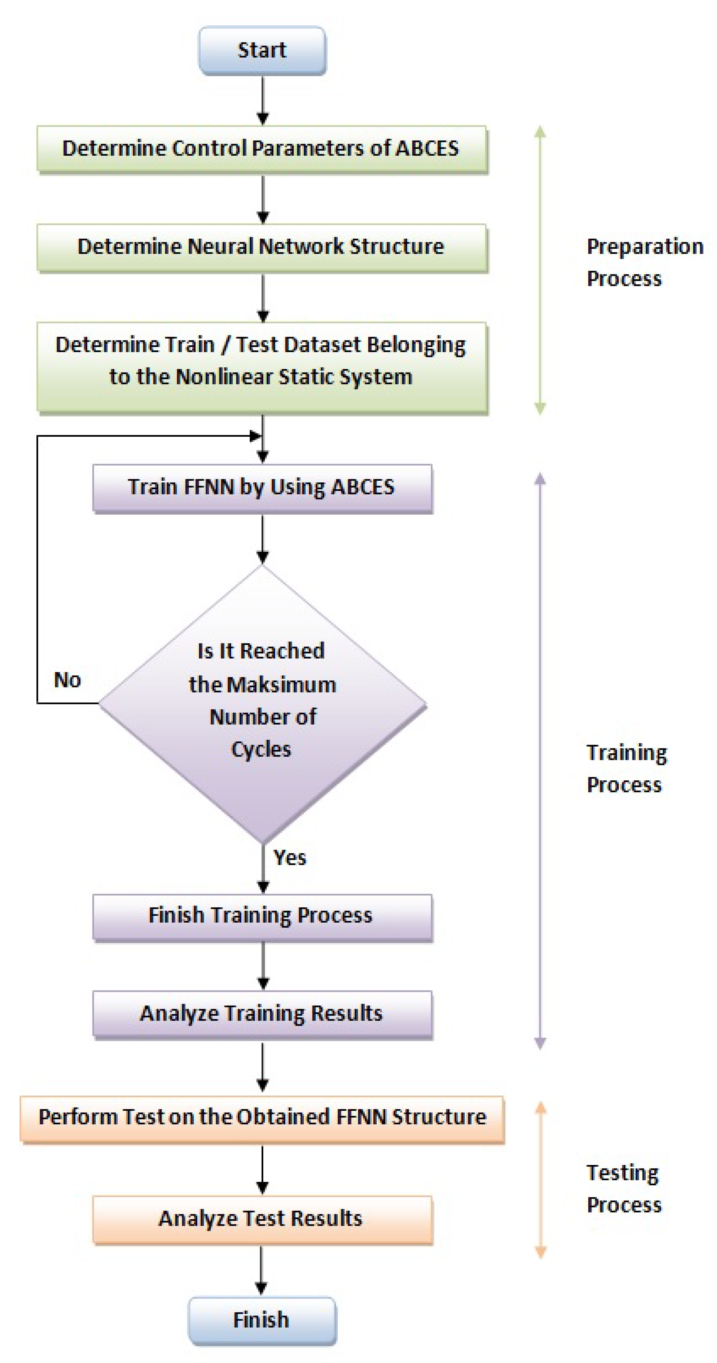In $S_5$ and $S_6$, 100 data points are used for the training process. The rest are chosen for testing. According to the dataset index value (i), mod (i, 5) = k operation is applied in all systems. If k = 0, the data is chosen for testing. Otherwise, it is included to dataset of the training process. There are two reasons for applying the mod operation according to 5 value: The first is to choose 80% of the dataset for the training process. In this case, the rest belong to the test dataset. It is ensured that the training dataset covers the whole dataset. This way, a more effective training process is realized. At the same time, the test dataset reflects the whole system. Feed forward neural network (FFNN) is used in this study. Sigmoid function is used for the neurons in the hidden layer and the output layer. Three different network structures are used for each system. 4, 8 and 12 neurons are used in the hidden layer. Training FFNN is realized via ABCES algorithm. Flow chart of FFNN training based on ABCES algorithm for the identification of nonlinear static systems is presented in Figure 2. Before the training, the input and output pairs of the nonlinear static system are normalized in the range of [0, 1]. For ABCES algorithm, population size and maximum number of iterations are taken as 20 and 5000, respectively. The number of training and test data used for each system is given in Table 9. MSE (mean squared error) calculated as in (9) is used as error value for training and testing process. Here, n is the number of samples. $y_i$ is real output and $\left({\overline{y}}_i\right)$ is predicted output. Each application is run 30 times to analyze it statistically. Mean error value (mean) and standard deviation (std) are obtained.

$$MSE=\frac{1}{n}\sum _{i=1}^n{(y_i-{\overline{y}}_i)}^2$$

(9)

The results obtained with the ABCES algorithm are presented in

Table 10. Results obtained with ABCES on nonlinear static system identification.

System	Network Structure	Train		Test
		Mean	Std	Mean	Std
S${}_1$	1-4-1	$1.16\times {10}^{-3}$	$4.86\times {10}^{-4}$	$2.21\times {10}^{-3}$	$7.65\times {10}^{-4}$
	1-8-1	$4.10\times {10}^{-4}$	$3.53\times {10}^{-4}$	$1.19\times {10}^{-3}$	$5.42\times {10}^{-4}$
	1-12-1	$2.73\times {10}^{-4}$	$1.64\times {10}^{-4}$	$1.12\times {10}^{-3}$	$5.81\times {10}^{-4}$
S${}_2$	2-4-1	$8.49\times {10}^{-4}$	$5.09\times {10}^{-4}$	$5.62\times {10}^{-3}$	$3.46\times {10}^{-3}$
	2-8-1	$2.52\times {10}^{-4}$	$1.03\times {10}^{-4}$	$2.47\times {10}^{-3}$	$1.62\times {10}^{-3}$
	2-12-1	$1.99\times {10}^{-4}$	$7.06\times {10}^{-5}$	$2.61\times {10}^{-3}$	$1.23\times {10}^{-3}$
S${}_3$	2-4-1	$6.45\times {10}^{-5}$	$3.64\times {10}^{-5}$	$2.57\times {10}^{-3}$	$1.16\times {10}^{-3}$
	2-8-1	$6.86\times {10}^{-5}$	$3.74\times {10}^{-5}$	$2.67\times {10}^{-3}$	$9.58\times {10}^{-4}$
	2-12-1	$7.03\times {10}^{-5}$	$3.33\times {10}^{-5}$	$3.06\times {10}^{-3}$	$2.21\times {10}^{-3}$
S${}_4$	3-4-1	$7.17\times {10}^{-4}$	$2.13\times {10}^{-4}$	$1.21\times {10}^{-3}$	$3.92\times {10}^{-4}$
	3-8-1	$4.35\times {10}^{-4}$	$1.87\times {10}^{-4}$	$9.50\times {10}^{-4}$	$3.88\times {10}^{-4}$
	3-12-1	$4.33\times {10}^{-4}$	$1.67\times {10}^{-4}$	$1.07\times {10}^{-3}$	$5.56\times {10}^{-4}$
S${}_5$	3-4-1	$3.59\times {10}^{-4}$	$1.74\times {10}^{-4}$	$3.06\times {10}^{-3}$	$3.69\times {10}^{-3}$
	3-8-1	$2.39\times {10}^{-4}$	$9.59\times {10}^{-5}$	$6.38\times {10}^{-3}$	$1.01\times {10}^{-2}$
	3-12-1	$2.41\times {10}^{-4}$	$9.06\times {10}^{-5}$	$6.74\times {10}^{-3}$	$7.21\times {10}^{-3}$
S${}_6$	4-4-1	$6.71\times {10}^{-4}$	$1.82\times {10}^{-4}$	$9.02\times {10}^{-4}$	$3.49\times {10}^{-4}$
	4-8-1	$4.56\times {10}^{-4}$	$1.46\times {10}^{-4}$	$8.42\times {10}^{-4}$	$8.09\times {10}^{-4}$
	4-12-1	$3.76\times {10}^{-4}$	$1.19\times {10}^{-4}$	$6.90\times {10}^{-4}$	$3.32\times {10}^{-4}$

. The increase in the number of neurons in the hidden layer in $S_1$ has increased the solution quality. The best mean error values for training and test are achieved with the 1-12-1 network structure. The number of neurons affects the mean training and test error values in $S_2$ differently. Although the best mean training error value is found with 2-12-1, the best mean test error value is obtained with 2-8-1. The low number of neurons in $S_3$ is more effective. The best mean error values for both training and test are achieved with 2-4-1. Close performance is observed in 3-8-1 and 3-12-1 network structures in $S_4$. Similarly, the best mean training error values for $S_5$ are found with 3-8-12 and 3-12-1. However, the best mean test error value is obtained by using 3-4-1. All the best results in $S_6$ are 4-12-1. When all systems are evaluated in general, it is possible to make four basic comments. First, network structure affects performance. Increasing or decreasing the number of neurons exhibits different behaviors depending on the system. Second, there is a difference between training and test errors. This situation can be explained by the selection of the training and test dataset. Third, generally low standard deviation values are obtained. This situation shows the stability of the solutions. Finally, the low error values found indicate that the ABCES algorithm is successful. 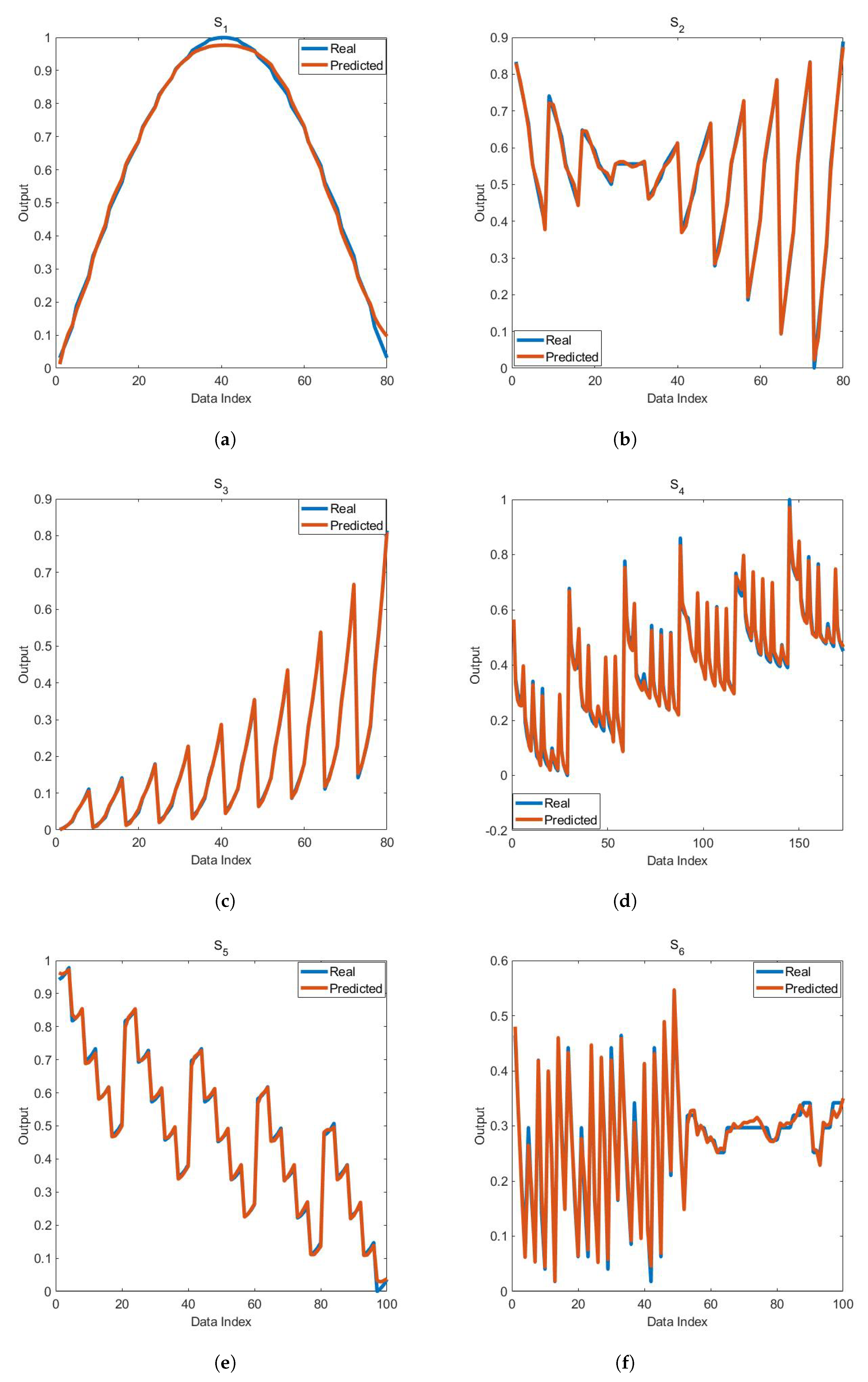In Figure 3, the graphs of the output found with ABCES algorithm and the real output are compared. It is seen that effective output graphics are obtained with ABCES algorithm in all systems. In fact, this is an indication that nonlinear static systems are identified with high accuracy.

It is compared with PSO, HS and ABC algorithm to better evaluate the performance of ABCES algorithm. The results are presented in

Table 11. Comparison of results found by using GA, PSO, HS, ABC and ABCES for on nonlinear static system identification based on neural network.

System	Network Structure	Train		Test
		Mean	Std	Mean	Std
S${}_1$	PSO	$2.08\times {10}^{-3}$	$6.86\times {10}^{-4}$	$3.26\times {10}^{-3}$	$1.17\times {10}^{-3}$
	HS	$1.29\times {10}^{-2}$	$7.38\times {10}^{-3}$	$1.44\times {10}^{-2}$	$8.17\times {10}^{-3}$
	ABC	$5.86\times {10}^{-4}$	$1.72\times {10}^{-4}$	$1.22\times {10}^{-3}$	$4.20\times {10}^{-4}$
	ABCES (Proposed)	$2.73\times {10}^{-4}$	$1.64\times {10}^{-4}$	$1.12\times {10}^{-3}$	$5.81\times {10}^{-4}$
S${}_2$	PSO	$1.95\times {10}^{-3}$	$8.65\times {10}^{-4}$	$7.56\times {10}^{-3}$	$3.55\times {10}^{-3}$
	HS	$2.50\times {10}^{-2}$	$1.00\times {10}^{-2}$	$3.94\times {10}^{-2}$	$1.82\times {10}^{-2}$
	ABC	$5.53\times {10}^{-4}$	$2.07\times {10}^{-4}$	$4.19\times {10}^{-3}$	$3.30\times {10}^{-3}$
	ABCES (Proposed)	$1.99\times {10}^{-4}$	$7.06\times {10}^{-5}$	$2.61\times {10}^{-3}$	$1.23\times {10}^{-3}$
S${}_3$	PSO	$8.17\times {10}^{-5}$	$3.35\times {10}^{-5}$	$3.74\times {10}^{-3}$	$1.29\times {10}^{-3}$
	HS	$1.21\times {10}^{-3}$	$7.68\times {10}^{-4}$	$8.43\times {10}^{-3}$	$4.73\times {10}^{-3}$
	ABC	$2.60\times {10}^{-4}$	$9.02\times {10}^{-5}$	$3.56\times {10}^{-3}$	$1.70\times {10}^{-3}$
	ABCES (Proposed)	$6.45\times {10}^{-5}$	$3.64\times {10}^{-5}$	$2.57\times {10}^{-3}$	$1.16\times {10}^{-3}$
S${}_4$	PSO	$1.96\times {10}^{-3}$	$9.17\times {10}^{-4}$	$2.31\times {10}^{-3}$	$7.28\times {10}^{-4}$
	HS	$9.28\times {10}^{-3}$	$8.00\times {10}^{-3}$	$8.71\times {10}^{-3}$	$7.41\times {10}^{-3}$
	ABC	$1.21\times {10}^{-3}$	$2.97\times {10}^{-4}$	$1.84\times {10}^{-3}$	$4.87\times {10}^{-4}$
	ABCES (Proposed)	$4.35\times {10}^{-4}$	$1.87\times {10}^{-4}$	$9.50\times {10}^{-4}$	$3.88\times {10}^{-4}$
S${}_5$	PSO	$4.88\times {10}^{-4}$	$3.38\times {10}^{-4}$	$2.16\times {10}^{-3}$	$4.01\times {10}^{-3}$
	HS	$2.94\times {10}^{-3}$	$1.45\times {10}^{-3}$	$8.58\times {10}^{-3}$	$5.24\times {10}^{-3}$
	ABC	$8.62\times {10}^{-4}$	$2.69\times {10}^{-4}$	$6.30\times {10}^{-3}$	$6.43\times {10}^{-3}$
	ABCES (Proposed)	$3.59\times {10}^{-4}$	$1.74\times {10}^{-4}$	$3.06\times {10}^{-3}$	$3.69\times {10}^{-3}$
S${}_6$	PSO	$2.72\times {10}^{-3}$	$1.44\times {10}^{-3}$	$2.61\times {10}^{-3}$	$1.33\times {10}^{-3}$
	HS	$1.58\times {10}^{-2}$	$7.14\times {10}^{-3}$	$1.65\times {10}^{-2}$	$9.56\times {10}^{-3}$
	ABC	$9.91\times {10}^{-4}$	$2.63\times {10}^{-4}$	$1.58\times {10}^{-3}$	$1.23\times {10}^{-3}$
	ABCES (Proposed)	$3.76\times {10}^{-4}$	$1.19\times {10}^{-4}$	$6.90\times {10}^{-4}$	$3.32\times {10}^{-4}$

. In $S_1$, the best mean training and test error values are found by ABCES algorithm. ABC algorithm is more effective after ABCES algorithm. The same is true for $S_2$. The best mean training error value in $S_3$ is found with ABCES. After ABCES, PSO is more effective. Although the best result in the mean test error value is obtained with ABCES, the worst results are found with HS. In $S_4$ it is clear that ABCES is effective. In $S_5$, the best mean training error value is found with ABCES, while the best mean test error value is obtained via PSO. The best results in $S_6$ are obviously found with ABCES. When the results are evaluated in general, ABCES algorithm is more successful in neural network training than others. After ABCES, the performances are listed as ABC algorithm, PSO and HS, respectively.

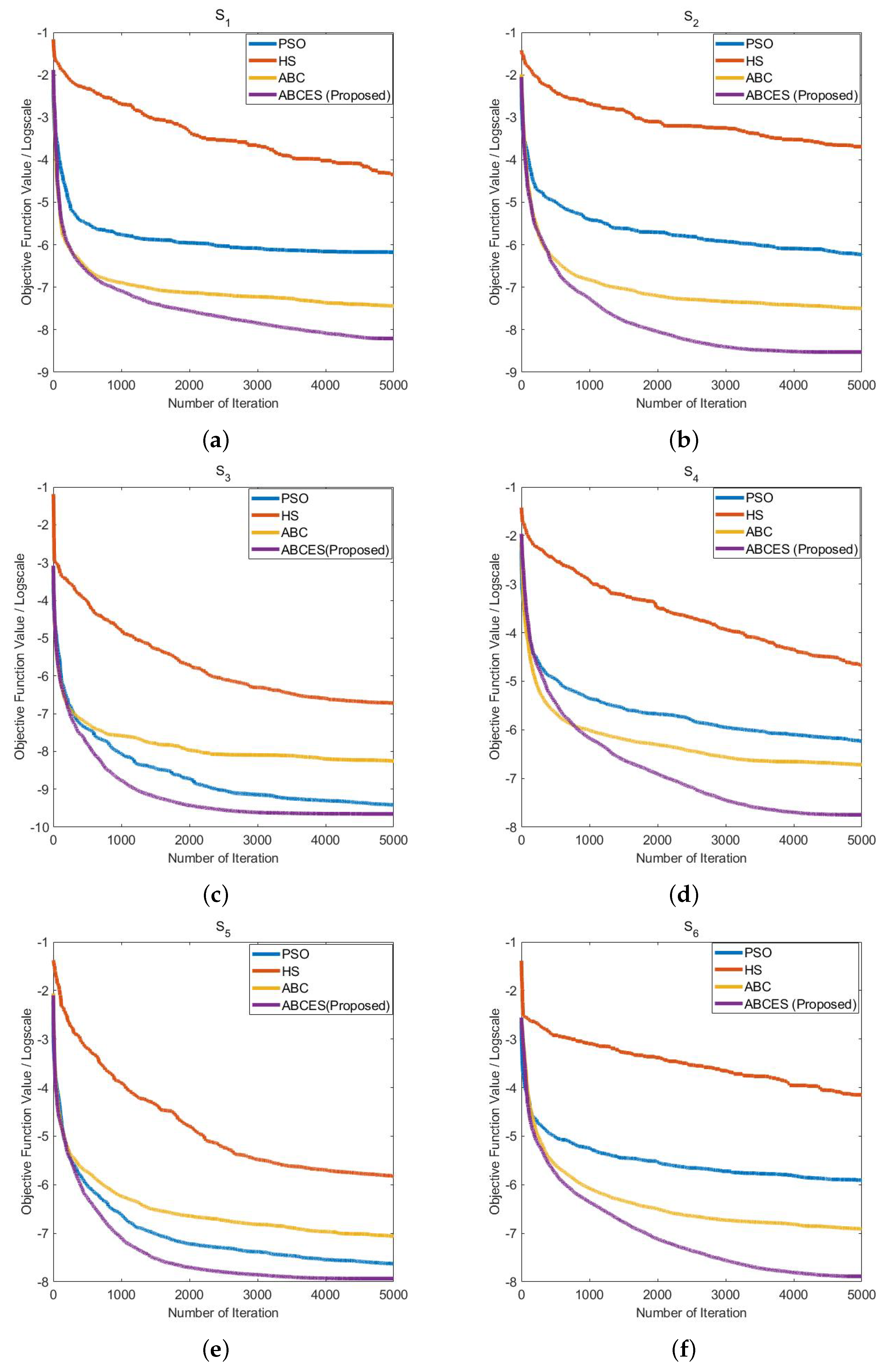
In Table 11, it is seen that the solution quality of ABCES algorithm is better than other algorithms. Besides the quality of the solution, the convergence speed is also important. Therefore, the convergence graphs of PSO, HS, ABC and ABCES on all systems are compared in Figure 4. It is observed that the convergence of ABCES algorithm is more effective on all systems. These graphics show that ABCES algorithm has better convergence speed than other algorithms. After the ABCES algorithm, the best convergence is achieved with the ABC algorithm, except $S_3$ and $S_5$. PSO has a more effective convergence than the ABC algorithm on $S_3$ and $S_5$.

5. Discussion

ABCES algorithm generates new solutions by using the information of previous solutions instead of random solution in the scout bee stage. “Limit” value is not fixed and is determined adaptively according to the number of iterations. How these changes affect the performance of ABCES algorithm is examined on two different problem groups: global optimization problems and FFNN training for the identification of nonlinear static systems.

The proposal of a new solution generation mechanism for the scout bee stage has been effective in solving global optimization problems. Many applications are realized in different number of evaluation and different problem dimensions. In these application results, it is observed that ABCES algorithm is generally more effective than ABC algorithm. Especially in high-dimensional problems, the performance of the algorithm has been significantly improved. The occurrence of a clear performance difference between the standard ABC algorithm and ABCES algorithm shows the effect of the scout bee stage and “Limit” control parameter. At the same time, it is seen that ABCES algorithm has more success in general compared to heuristics such as GA, PSO and DE. This is an indication that ABCES algorithm can compete with different heuristic algorithms. ABCES algorithm also finds low standard deviation values parallel to the low error value. This shows that the results are robust.

The identification of nonlinear static systems is one of the difficult problems due to system behavior. The effect of changes on both the scout bee stage and the “limit” control parameter are analyzed on 6 nonlinear static systems. Generally, as the number of neurons in the hidden layer increases, more effective results are obtained. This situation shows that the problem is difficult, and it reveals the necessity of more weight values to explain the relationship. With ABCES algorithm, a performance increase of 50% and above has been achieved in all systems compared to ABC algorithm. The changes in the scout bee stage have increased the convergence speed of ABCES algorithm. ANN training aims to find the closest output to the real output. It is seen from the analyzes that ABCES algorithm is an effective training algorithm in this regard. It is compared with heuristics such as PSO, HS and ABC to better understand the success of ABCES algorithm. The results show that ABCES algorithm is successful in FFNN training.

It is seen that the changes realized on the scout bee stage and limit control parameter with ABCES algorithm positively affect the result. Different solution-generating mechanisms for the scout bee stage can be integrated to further improve the performance of ABCES algorithm. At the same time, different approaches can be put forward to determine “limit” control parameter adaptively.

6. Conclusions

This paper proposes a neural network-based approach for the identification of nonlinear static systems. A new training algorithm called ABCES (ABC Based on Effective Scout Bee Stage) is introduced to achieve effective results in modeling with artificial neural networks. Standard ABC algorithm basically consists of three stages: employed bee, onlooker bee and scout bee. Employed and onlooker bee stages are more efficient than the scout bee stage. When the scout bee stage is reached, it is understood that better new solution is not developed. In this case, a random solution is created in the scout bee stage of standard ABC algorithm. In fact, this means failure to use of information obtained. If this is prevented, a more effective algorithm will be created. For this purpose, ABCES algorithm is proposed to create a more effective scout bee stage. In this algorithm, two important changes are made according to standard ABC algorithm. First, “limit” control parameter is set to adaptive according to the number of iterations. Secondly, a new solution generation mechanism that enables the adjustment of the new position according to the global best solution in the scout bee stage, is proposed. With these changes, an effective ABCES algorithm has been created. The performance of ABCES algorithm is evaluated on two different problem groups. First, the applications are realized on 13 numerical optimization test problems. It is compared with GA, PSO, DE and ABC algorithms. The Wilcoxon signed rank test is applied to determine the significance of the results. The results show that ABCES algorithm is generally more successful than other algorithms in solving numerical optimization problems.

Secondly, FFNN is trained by using ABCES algorithm for the identification nonlinear static systems. Six nonlinear static systems are used in the applications. The effect of different network structures on performance is examined. The performance of ABCES algorithm is compared with PSO, HS and ABC algorithm in terms of solution quality and speed of convergence. The results show that ABCES algorithm is generally more successful than other algorithms in the identification of nonlinear static systems based on neural networks.

In this study, ABCES algorithm is used first time and it is evaluated on global optimization problems and training FFNN. In future studies, it is possible to examine the performance of ABCES algorithm on different types of problems. As a continuation of this study, FFNN training can be performed by using ABCES algorithm to identify nonlinear dynamic systems. Additionally, neuro-fuzzy models can be trained with ABCES algorithm to identify nonlinear dynamic and static systems. Its performance on neuro-fuzzy training can be evaluated. Apart from system identification, ANN and neuro-fuzzy training can be carried out with ABCES for the solution of real-world problems.

References

1. Fister, I., Jr.; Yang, X.-S.; Fister, I.; Brest, J.; Fister, D. A brief review of nature-inspired algorithms for optimization. arXiv 2013, arXiv:1307.4186v1. [Google Scholar]
2. Karaboga, D.; Kaya, E. Training ANFIS by using the artificial bee colony algorithm. Turk. J. Electr. Eng. Comput. Sci. 2017, 25, 1669–1679. [Google Scholar] [CrossRef]
3. Karaboga, D.; Kaya, E. Training ANFIS Using Artificial Bee Colony Algorithm for Nonlinear Dynamic Systems Identification. In Proceedings of the 22nd Signal Processing and Communications Applications Conference (SIU), Trabzon, Turkey, 23–25 April 2014; IEEE: Piscataway, NJ, USA, 2014. [Google Scholar]
4. Karaboga, D.; Kaya, E. An adaptive and hybrid artificial bee colony algorithm (aABC) for ANFIS training. Appl. Soft Comput. 2016, 49, 423–436. [Google Scholar] [CrossRef]
5. Karaboga, D.; Kaya, E. Training ANFIS by using an adaptive and hybrid artificial bee colony algorithm (aABC) for the identification of nonlinear static systems. Arab. J. Sci. Eng. 2019, 44, 3531–3547. [Google Scholar] [CrossRef]
6. Karaboga, D.; Ozturk, C. Neural networks training by artificial bee colony algorithm on pattern classification. Neural Netw. World 2009, 19, 279. [Google Scholar]
7. Horng, M.-H. Multilevel thresholding selection based on the artificial bee colony algorithm for image segmentation. Expert Syst. Appl. 2011, 38, 13785–13791. [Google Scholar] [CrossRef]
8. Karaboga, N. A new design method based on artificial bee colony algorithm for digital IIR filters. J. Frankl. Inst. 2009, 346, 328–348. [Google Scholar] [CrossRef]
9. Yeh, W.-C.; Hsieh, T.-J. Solving reliability redundancy allocation problems using an artificial bee colony algorithm. Comput. Oper. Res. 2011, 38, 1465–1473. [Google Scholar] [CrossRef]
10. Hemamalini, S.; Simon, S.P. Artificial bee colony algorithm for economic load dispatch problem with non-smooth cost functions. Electr. Power Components Syst. 2010, 38, 786–803. [Google Scholar] [CrossRef]
11. Hong, W.-C. Electric load forecasting by seasonal recurrent SVR (support vector regression) with chaotic artificial bee colony algorithm. Energy 2011, 36, 5568–5578. [Google Scholar] [CrossRef]
12. Şahin, A.Ş. Optimization of solar air collector using genetic algorithm and artificial bee colony algorithm. Heat Mass Transf. 2012, 48, 1921–1928. [Google Scholar] [CrossRef]
13. Zaman, M.A.; Gaffar, M.; Alam, M.M.; Mamun, S.A.; Matin, M.A. Synthesis of antenna arrays using artificial bee colony optimization algorithm. Int. J. Microw. Opt. Technol. 2011, 6, 234–241. [Google Scholar]
14. Deng, X. An efficient hybrid artificial bee colony algorithm for customer segmentation in mobile E-commerce. J. Electron. Commer. Organ. (JECO) 2013, 11, 53–63. [Google Scholar] [CrossRef]
15. Bulut, O.; Tasgetiren, M.F. An artificial bee colony algorithm for the economic lot scheduling problem. Int. J. Prod. Res. 2014, 52, 1150–1170. [Google Scholar] [CrossRef]
16. Bansal, J.C.; Sharma, H.; Jadon, S.S. Artificial bee colony algorithm: A survey. Int. J. Adv. Intell. Paradig. 2013, 5, 123–159. [Google Scholar] [CrossRef]
17. Karaboga, D.; Gorkemli, B.; Ozturk, C.; Karaboga, N. A comprehensive survey: Artificial bee colony (ABC) algorithm and applications. Artif. Intell. Rev. 2014, 42, 21–57. [Google Scholar] [CrossRef]
18. Ozturk, C.; Hancer, E.; Karaboga, D. Color image quantization: A short review and an application with artificial bee colony algorithm. Informatica 2014, 25, 485–503. [Google Scholar] [CrossRef] [Green Version]
19. Bansal, J.C.; Sharma, H.; Arya, K.; Deep, K.; Pant, M. Self-adaptive artificial bee colony. Optimization 2014, 63, 1513–1532. [Google Scholar] [CrossRef]
20. Babaeizadeh, S.; Ahmad, R. An efficient artificial bee colony algorithm for constrained optimization problems. J. Eng. Appl. Sci. 2014, 9, 405–413. [Google Scholar]
21. Draa, A.; Bouaziz, A. An artificial bee colony algorithm for image contrast enhancement. Swarm Evol. Comput. 2014, 16, 69–84. [Google Scholar] [CrossRef]
22. Karaboga, D.; Gorkemli, B. A quick artificial bee colony (qABC) algorithm and its performance on optimization problems. Appl. Soft Comput. 2014, 23, 227–238. [Google Scholar] [CrossRef]
23. Gao, W.-F.; Liu, S.-Y.; Huang, L.-L. Enhancing artificial bee colony algorithm using more information-based search equations. Inf. Sci. 2014, 270, 112–133. [Google Scholar] [CrossRef]
24. Wang, B. A novel artificial bee colony algorithm based on modified search strategy and generalized opposition-based learning. J. Intell. Fuzzy Syst. 2015, 28, 1023–1037. [Google Scholar] [CrossRef]
25. Kıran, M.S.; Fındık, O. A directed artificial bee colony algorithm. Appl. Soft Comput. 2015, 26, 454–462. [Google Scholar] [CrossRef]
26. Liang, J.-H.; Lee, C.-H. A modification artificial bee colony algorithm for optimization problems. Math. Probl. Eng. 2015, in press. [Google Scholar] [CrossRef] [Green Version]
27. Babaeizadeh, S.; Ahmad, R. Enhanced constrained artificial bee colony algorithm for optimization problems. Int. Arab J. Inf. Technol. 2017, 14, 246–253. [Google Scholar]
28. Li, G.; Cui, L.; Fu, X.; Wen, Z.; Lu, N.; Lu, J. Artificial bee colony algorithm with gene recombination for numerical function optimization. Appl. Soft Comput. 2017, 52, 146–159. [Google Scholar] [CrossRef]
29. Ozturk, C.; Hancer, E.; Karaboga, D. A novel binary artificial bee colony algorithm based on genetic operators. Inf. Sci. 2015, 297, 154–170. [Google Scholar] [CrossRef]
30. Yaghoobi, T.; Esmaeili, E. An improved artificial bee colony algorithm for global numerical optimisation. Int. J. Bio-Inspired Comput. 2017, 9, 251–258. [Google Scholar] [CrossRef]
31. Dreiseitl, S.; Ohno-Machado, L. Logistic regression and artificial neural network classification models: A methodology review. J. Biomed. Inform. 2002, 35, 352–359. [Google Scholar] [CrossRef] [Green Version]
32. Lisboa, P.J.; Taktak, A.F. The use of artificial neural networks in decision support in cancer: A systematic review. Neural Netw. 2006, 19, 408–415. [Google Scholar] [CrossRef]
33. Tealab, A. Time series forecasting using artificial neural networks methodologies: A systematic review. Future Comput. Inform. J. 2018, 3, 334–340. [Google Scholar] [CrossRef]
34. Dase, R.K.; Pawar, D.D. Application of artificial neural network for stock market predictions: A review of literature. Int. J. Mach. Intell. 2010, 2, 14–17. [Google Scholar]
35. Dhillon, A.; Verma, G.K. Convolutional neural network: A review of models, methodologies and applications to object detection. Prog. Artif. Intell. 2020, 9, 85–112. [Google Scholar] [CrossRef]
36. Capizzi, G.; Lo Sciuto, G.; Napoli, C.; Tramontana, E. A multithread nested neural network architecture to model surface plasmon polaritons propagation. Micromachines 2016, 7, 110. [Google Scholar] [CrossRef] [Green Version]
37. Sciuto, G.L.; Susi, G.; Cammarata, G.; Capizzi, G. A Spiking Neural Network-Based Model for Anaerobic Digestion Process. In Proceedings of the 2016 International Symposium on Power Electronics, Electrical Drives, Automation and Motion (SPEEDAM), Anacapri Capri Island, Italy, 22–24 June 2016; IEEE: Piscataway, NJ, USA, 2016. [Google Scholar]
38. Capizzi, G.; Sciuto, G.L.; Woźniak, M.; Damaševicius, R. A Clustering Based System for Automated Oil Spill Detection by Satellite Remote Sensing. In Proceedings of the International Conference on Artificial Intelligence and Soft Computing, Zakopane, Poland, 12–16 June 2016; Springer: Cham, Switzerland, 2016. [Google Scholar]
39. Mohmad Hassim, Y.M.; Ghazali, R. An improved functional link neural network learning using artificial bee colony optimisation for time series prediction. Int. J. Bus. Intell. Data Min. 2013, 8, 307–318. [Google Scholar]
40. Zhang, Y.; Wu, L.; Wang, S. Magnetic resonance brain image classification by an improved artificial bee colony algorithm. Prog. Electromagn. Res. 2011, 116, 65–79. [Google Scholar] [CrossRef] [Green Version]
41. Ozkan, C.; Kisi, O.; Akay, B. Neural networks with artificial bee colony algorithm for modeling daily reference evapotranspiration. Irrig. Sci. 2011, 29, 431–441. [Google Scholar] [CrossRef]
42. Chen, S.; Fang, G.; Huang, X.; Zhang, Y. Water quality prediction model of a water diversion project based on the improved artificial bee colony–backpropagation neural network. Water 2018, 10, 806. [Google Scholar] [CrossRef] [Green Version]
43. Karaboga, D.; Basturk, B. A powerful and efficient algorithm for numerical function optimization: Artificial bee colony (ABC) algorithm. J. Glob. Optim. 2007, 39, 459–471. [Google Scholar] [CrossRef]
44. Karaboga, D.; Akay, B. A comparative study of artificial bee colony algorithm. Appl. Math. Comput. 2009, 214, 108–132. [Google Scholar] [CrossRef]
Figure 1. General structure of an artificial neuron.
Symmetry 13 00419 g001
Figure 2. Flowchart for FFNN training based on ABCES algorithm for the identification of nonlinear static systems.
Symmetry 13 00419 g002
Figure 3. Comparison of real and predicted outputs for (a) S 1 (b) S 2 (c) S 3 (d) S 4 (e) S 5 (f) S 6 .
Symmetry 13 00419 g003
Figure 4. Comparison of convergences of PSO, HS, ABC and ABCES on (a) S 1 (b) S 2 (c) S 3 (d) S 4 (e) S 5 (f) S 6 .
Symmetry 13 00419 g004