
TIN Surface and Radial Viewshed Determination Algorithm Parallelisation on Multiple Computing Machines


Graphics and High Performance Computing Group, Department of Computer Science, Faculty of Computer Science and Telecommunications, Cracow University of Technology, Warszawska st 24, 31-155 Cracow, Poland
*
Author to whom correspondence should be addressed.
Symmetry 2021, 13(3), 424; https://0-doi-org.brum.beds.ac.uk/10.3390/sym13030424
Submission received: 2 February 2021
/
Revised: 2 March 2021
/
Accepted: 3 March 2021
/
Published: 6 March 2021
(This article belongs to the Section Computer)
Abstract
:In this paper we have proposed a method of solving the computer graphic problem of creating a Triangulated Irregular Network (TIN) surface in large clouds in order to create viewsheds. The method is based on radial TIN surface and viewshed visualization task subdivision using multiple computing machines, which is intended to accelerate the process of generating the complete viewshed.
1. Introduction
Engineers who perform analytical and design tasks utilise software tools that often run on advanced workstations. Sophisticated tool systems have a very broad range of functionality, but sometimes lack sufficient effectiveness to compute new data types, such as 3D point clouds. Often, specific types of data can be entered into engineering tool systems, but their amount makes further work ineffective. This can be solved by subdivision, applied both to the functional and spatial scope. Partial calculations can be performed on multiple computers and thus accelerated. In this paper, we propose a solution that can be successfully applied using different equipment configurations and tasks in which there is a need to process large datasets. The case presented here is the problem of generating terrain models in representations of Triangulated Irregular Network (TIN) surfaces [1] on an extensive 3D point cloud, whose size does not allow for single-process calculation.
A point cloud is a set of points in three-dimensional space. Each point is determined by X, Y, Z, coordinates, and may contain colour information in the form of an RGB value. There are many methods dedicated to the acquisition of point cloud data. For small-size point clouds, one can use 3D scanners. In the case of large clouds, photogrammetry and LIDAR scanning are preferable [2,3,4]. The cloud examined and processed in this study was obtained by means of LIDAR scanning, as a part of the ISOK project (IT System of the Country Protection). As much as 98% of Poland’s territory was scanned during this project, with a density between 6–12 points/m.
The point cloud is available in the form of LAS files, in which each point is represented by X, Y, Z, coordinates, RGB colour and assigned to one of four classes: ground, building, water and vegetation [5]. Viewsheds are generated based on TIN surfaces [6]. The viewshed is a way to determine areas in a certain space from which a given point is visible and, simultaneously, the areas that are visible from the given point. In its simplest form, the viewshed is generated from a singular, specific viewpoint. Visibility maps are an extension of viewsheds and are generated from numerous points, which can be in the range of hundreds of thousands when creating a visibility map for large objects like a mountain range. A viewshed is generated for each point, and the resulting map is a composition of multiple viewsheds; it contains combined information about visibility. Viewsheds and visibility maps are used in road design, urban design, spatial and strategic planning, nature conservation, monument preservation and military science. This data is in the form of rasters, which allows it to be easily compiled with other data layers in CAD and GIS applications.
2. Software Performance Enhancement Methods
To ensure proper and effective software operation, the team of programmers that write it must use dedicated code writing principles and adhere to the latest solutions so that software can meet user expectations. Key principles include maintaining legible code structure, the application of proper variable types, applying indicators, programming patterns, etc. The art of software creation is perfected along with the emergence of new programming concepts and technologies [7].
When all available source code optimization methods are used and performance remains unsatisfactory, it can be parallelised, i.e., subdivided into subtasks that can be distributed across different processor threads [8] or cores. There are numerous technologies distinguished here, including OpenMP [9,10], MPI [11] or CUDA [12]. Each have their advantages and disadvantages and are dedicated to solving different task types. Not all tasks can be parallelised. Typically, this can be done only with tasks whose subtasks can be performed independently, i.e., the computing outputs of some are not required to begin others.
In cases when all performance enhancement methods have been applied, the code is optimal, parallelised and all computer resources are engaged, subtask distribution can be extended to other computers. In this case, processes that fully utilize multi-core architecture can be distributed. The proposed method allows for the distribution of tasks performed by well-known engineering software applications. However, many of these applications perform each task on individual cores. In this case, the same, or slightly modified, subtask distribution procedures used to distribute them to multiple computers can be applied to distribute them to available processors or processor cores.
3. Sample Task Overview
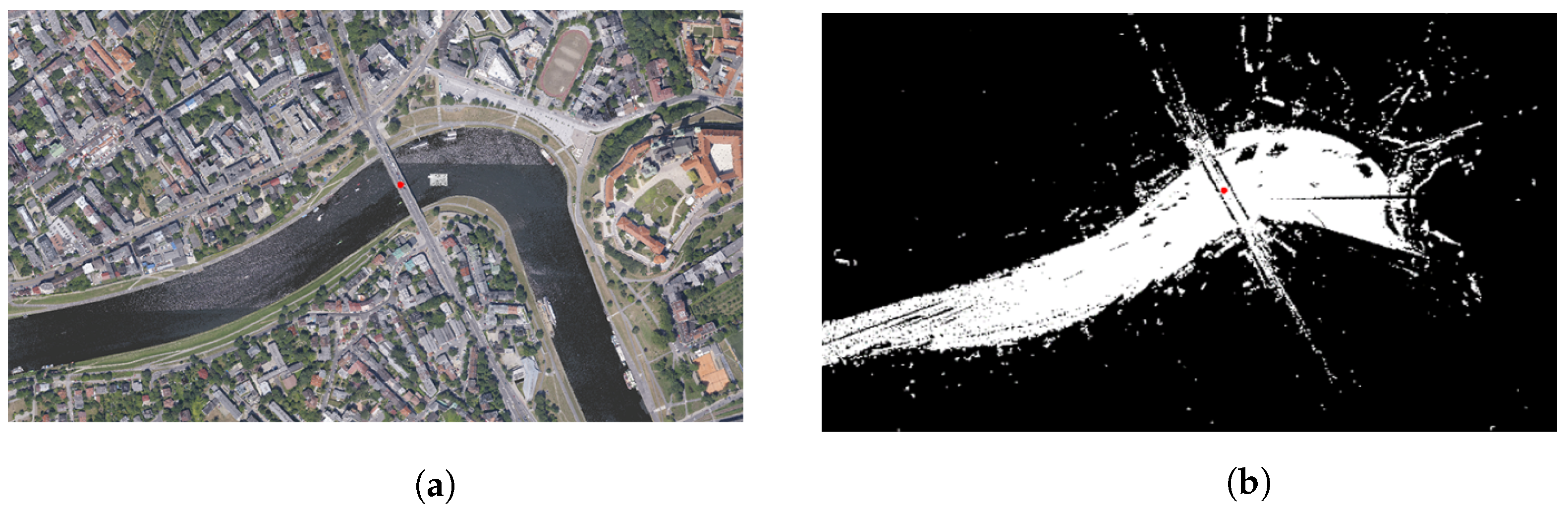
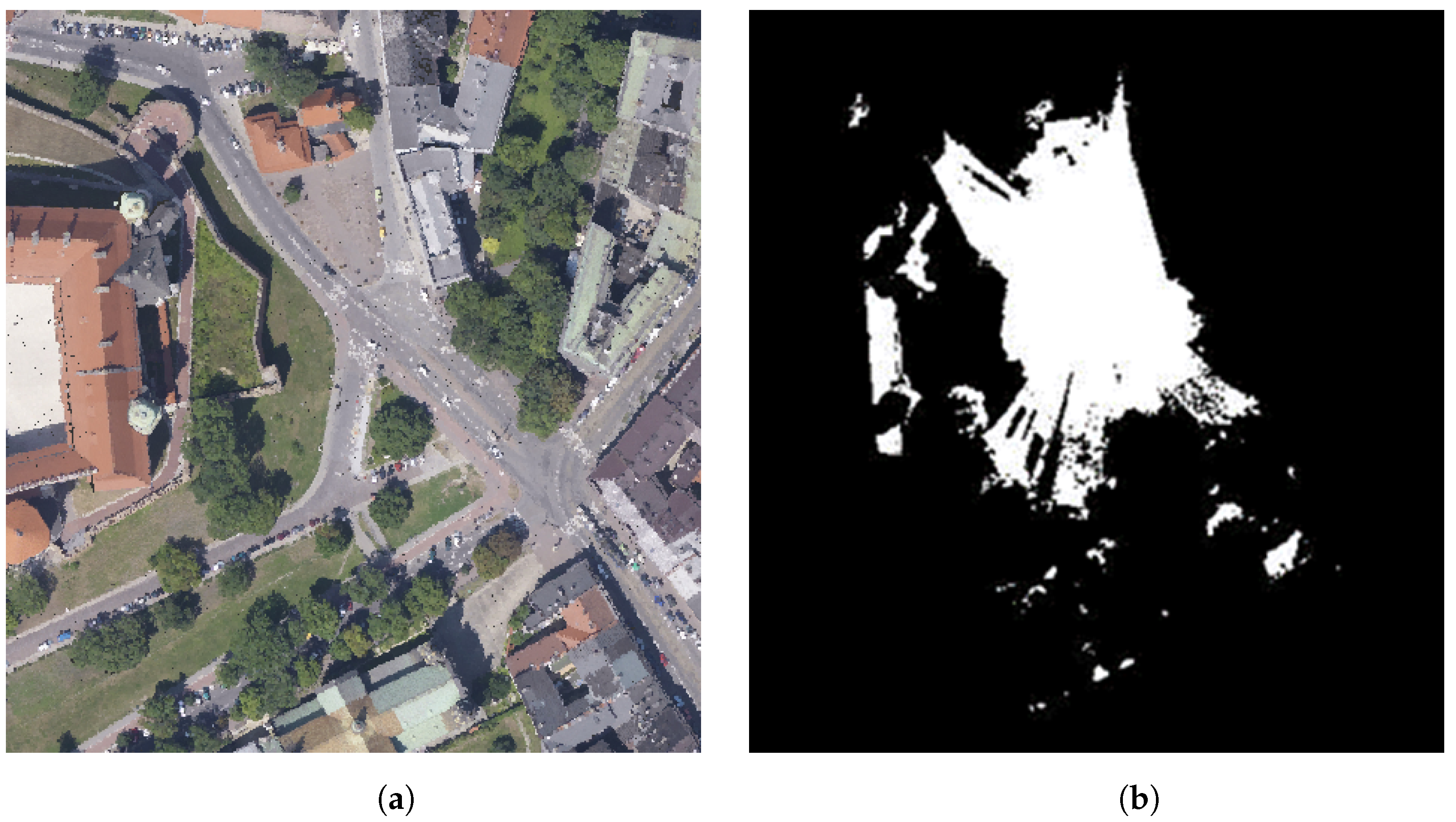
In this paper, we have presented a method that allows the processing of large datasets via an application that is commonly used by engineers in everyday work. In this application, it is not possible to process such a large dataset on an individual workstation in an acceptable timeframe. The method is presented on the example of a task that generates visibility charts in three-dimensional terrain model environments comprising dense point clouds. Visibility charts (Figure 1a,b) are graphical representations of space that are either visible or not visible from a given location. We also distinguish visibility maps, which are compilations of multiple visibility charts created based on different points.
Viewsheds are used in spatial analyses by, among others, urbanists, landscape architects and spatial planning professionals [13]. One of the methods used to generate them is based on the orthogonal rendering of a three-dimensional terrain model with a point light source placed at the location for which the viewshed is generated. The terrain model and cover should be represented by objects that obstruct light—preferably using a TIN representation. Setting a point light source with an indefinite illumination range at the location for which the viewshed is prepared results in the illumination of objects visible from said location. When raytracing is used to model light, the precision of the viewshed becomes proportional to the accuracy of the space’s geometric model and the resolution of the rendering.
The precision of the geometric model is dependent on the type of spatial data. The most precise data is provided by point clouds produced by LIDAR scans [14,15]. Point clouds [16]—are sets of points in three-dimensional space. Every point is defined by coordinates x, y, z in a given coordinate system. Apart from location information, every point can include additional information, such as RGB colour and class. The LAS [5] specification distinguishes four main classes: ground—which includes points on the ground; building—points that represent buildings; water—which represents water surfaces, and vegetation—points representing tall greenery.
The point cloud used in the study presented in this paper was obtained as a part of the ISOK project [17] in standard II, which requires 6–12 pt/m of real-world space. This is highly accurate spatial data. It is in immense demand among specialist designers and analysts who focus on urban space. However, their use often leads to numerous problems. Points, as non-dimensional objects, do not reflect traced rays in a visibility function. It is the result of rays penetrating between points. A closed surface is not created on the vertices, so the rays are not able to reflect. To produce a visibility chart, one must generate a polygonal mesh out of the point cloud. Here, the enormous amount of points becomes an obstacle. Landscape-scale visual analysis requires large areas to be modelled (e.g., 15 km × 20 km), and whose areas contain billions of individual points. Polygonal meshes should comprise a similar number of triangles. Computer systems used by these specialists are unable to generate such extensive meshes in an acceptable timeframe.
4. Dividing Tasks into Subtasks
Generating a viewshed is based on building a 3D geometric model of a space, producing a rendering with a single point-based light source at the observation point and thresholding the render image with a threshold set so that all illuminated places take on a positive value and all non-illuminated places take on a negative value. Typically, they are marked in black and white on the charts. In cases where a viewshed cannot be plotted due to the mesh being too dense, the model can be subdivided into radial sections [18]. The division of point clouds into radial sections is performed by projecting the cloud onto a 2D surface followed by radial sectioning following an angular radius. There can be any number of sections, which is dependent on the angular division selected. This number is entered by the user. A detailed overview of radial division has been presented in the paper. To accelerate the division, we applied an algorithm using a k-d tree (2D tree) along with a subtree rejection algorithm that has been presented in [6].
Their angular scope defines the size of the mesh section and the number of sections (inversely proportional). Viewsheds are compiled into maps which, for instance, display visibility from a given road. They show sections from which elements of space are visible, including extensive objects such as mountain chains, and how much of them can be seen. Numerous points are systematically distributed along the length of a road or on the surface of extensive objects. Their viewsheds, through matric summation, comprise visibility maps.
There are multiple ways in which these processes can be parallelised. Radial sections and individual viewsheds that form visibility maps are generated in separate processes. In cases where they are generated in model environments that consist of dense point clouds on workstations dedicated to engineering tasks, one must perform very fine divisions. To address this problem, an algorithm that subdivides the point cloud into radial sections from the central point was created, with the objective of creating smaller TIN surfaces. Fragmentary viewsheds are generated on these surfaces, as is their subsequent combination, which results in a complete viewshed.
The simplest process of subdividing the point cloud into radial sections, i.e., point by point, is very time-consuming. To further simplify it, we propose changing the storage structure of these points into a k-d tree, for which a novel tree rejection algorithm has been implemented. The algorithm outputs several small clouds, for which TIN surfaces re then generated. In the case of using a single computer, this can take a very long time, as every surface and chart creation operation is performed sequentially.
We can distinguish the following subtasks within visibility map and viewshed creation (Figure 2):
- Subdivision of the point cloud into radial sections
- Generation of a mesh in each radial section
- Rendering of each radial section
- Combining viewsheds from renderings of each section
- Matrix calculation of selected charts into a visibility map
4.1. Parallelization Method Proposal
In the case presented, we generate a viewshed via dividing point clouds into radial sections. Each section is then sent to one of multiple computing machines (Figure 3), where each machine is responsible for creating a three-dimensional TIN surface and generating a fragment of the viewshed. After this process concludes, the charts are returned to the main computer as components. During the final stage, all partial charts are combined into a single main chart, which solves the problem fully.
4.2. Program Operation Course
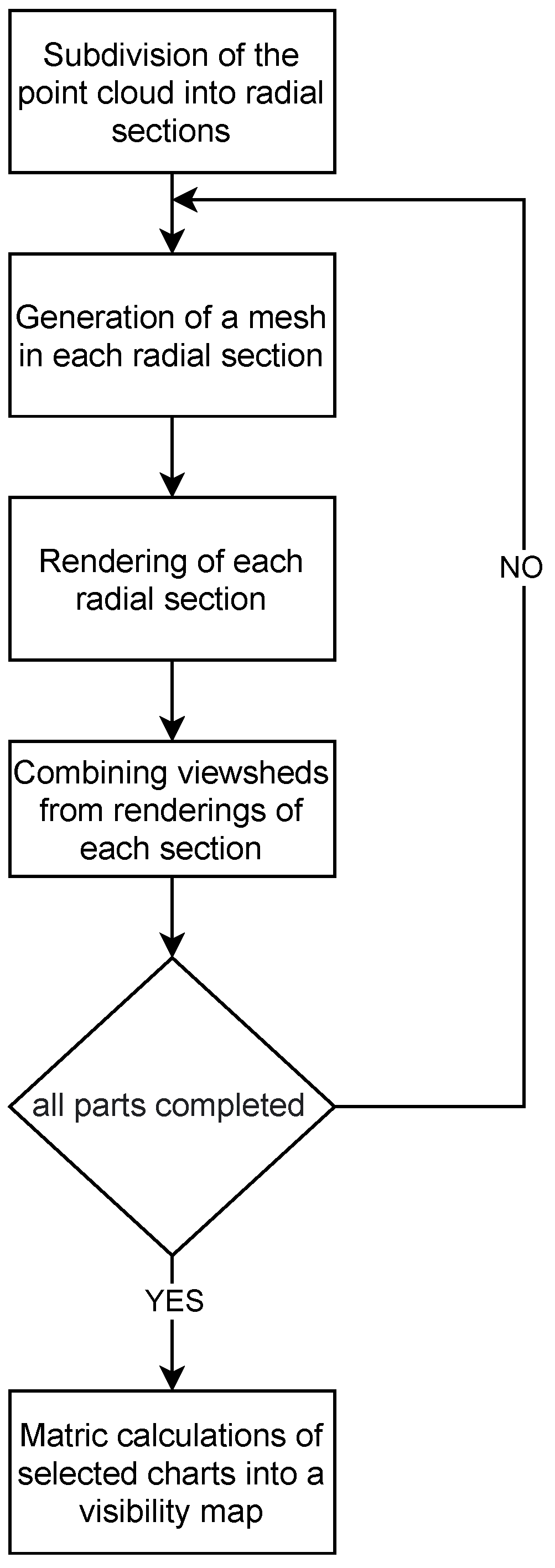
The first step taken by the program is the creation of a k-d tree, the second is the determination of small radial sections of the point cloud. Afterwards, it sends a header with information about the cloud and rendering method to each computer, along with sending N clouds to M computers. The structure of the radial section generation algorithm subdivides cloud after cloud, so there is no need to wait for all clouds to be created prior to the start of the transfer process. If a subsequent section is available, it is immediately processed. After completing every viewshed for every section, they are combined on the main computer into one viewshed. The entire process will be presented on the block diagram below (Figure 4).
4.3. Header File Description
For the program to properly function, every time it is run, a package is sent to each computer with a header file, a template (.dwt) with basic drawing environment parameters and a batch file (.bat) that runs the engineering program on node computers.
- Header file, which contains:
- –
- Coordinates for the point for which the viewshed is generated,
- –
- Rendering quality, scope and resolution parameters,
- –
- File names.
- The batch file that runs the program that awaits tasks and the program for TIN surface generation, which is Autocad Civil 3D ® [19],
- A script that runs in Autocad Civil 3D ®,
- A library with functions necessary for automatic surface generation, rendering and saving.
4.4. Overview of Tasks Assigned to Specific Computers
MOTHER COMPUTER—overview of processes performed on the main computer.
Input data—point cloud
- K-d tree execution
- Section number and angular scope determination
- Node computer number and access determination
- Package distribution
- Generation of N clouds and distribution to node computers
- Rendering reception
- Combination of partial viewsheds into a complete viewshed
Output data—complete viewshed
NODE COMPUTERS—overview of processes performed on N available computers.
Input data—partial cloud in a radial section
- Receipt of the header file with render and central point specification
- Receipt of point cloud section
- Viewshed execution
- Viewshed return with information about task conclusion
- Standby for another cloud/information about the completion of the entire process.
Output data—viewshed on a radial section
4.5. Technology
To create a program with the best possible performance, we used several technologies to make it user friendly, comply with software development principles and address the problem for which it has been created.
- C++ programming language [20]—the program that creates the k-d tree, divides the cloud and generates smaller clouds.
- AutoCad CIVIL 3D ® —for generating TIN surfaces and the viewshed.
- C# programming language [21]—to automate operations performed in Civil 3D ®
- Batch program [22]—for the automatic execution of the program on node computers.
5. Comparison of Algorithm Execution Times with the Use of Different Parallelization Methods
Methods derived from using the algorithm have been presented by conducting experiments with different cases of its execution. Shortening task execution times were observed while comparing the times obtained while using a single computing machine with limiting computer core number and with maximum load across all nodes. Times for sequential and parallel task execution were presented for different processor uses. Afterwards, we tested the use of different computer numbers. The experiments were performed on computers with the following parameters: Computer parameters:
- Operating system—Windows 10 64 bit
- Processor— i7-4760HQ 2.10–3.30 GHz
- RAM—16 GB DDR3L 1333 MHz/1600 MHz
- Drive—SSD
Available online: (accessed on 15 March 2012) Two tasks were formulated for the experiments.
Task 1, executed in the point cloud, marked with the letter (A), which consists of 82 × points. In this case, we analyzed task execution times for a single computer with varied processor use. The analysis covered both sequential and parallel algorithm operation. In the case of task 2, we applied the technology presented in the paper, which utilizes multiple computers. The algorithm was executed in parallel on multiple computers that operated sequentially. We used two point clouds. Cloud (B), with a number of points equal to 76 × , and a larger point cloud (C), whose number of points was 27 × . In addition, we investigated different numbers of point cloud sections: a division into 10 and 16 sections. Due to changes in subdivision, we presented the dependency between task performance time and the amount of parts calculated. We did not test the point cloud from task 1 in this manner, as the number of points in that cloud was small enough that the application of multiple computers with this algorithm would only extend calculation time.
5.1. Task 1: Subdivision of Point Cloud (A) into Four Parts
Case 1: The task was performed on a single computer with the use of a varying number of processor cores. Four point cloud parts were processed sequentially, one after another (Table 1).
This case demonstrated that sequential task performance time decreased as the number of engaged processor cores increased
Case 2: Task 1 was performed on a single computer with the use of different numbers of processor cores. The task was performed in parallel, with four clouds processed simultaneously (Table 2).
This case shows how parallel task performance time decreased along with the number of processor cores engaged. An observably substantial amount of time was saved here relative to case 1, wherein every part waited for the previous part to finish processing. In case 2, all were processed simultaneously. In this case, the size of each section is important. They were small enough that the computer, while creating TIN surfaces in parallel, had sufficient leftover operating memory and was able to process them all. Concerning parts with greater point numbers, there is a risk that parallel processing may not be performed. In such cases, one has to use the method shown in case 1, which is more time-consuming, but has the capacity to assign more processing power to a single part.
To better analyze the results presented above (Table 3), we present a comparison of calculation times for one part of cloud (A) on one core with the time of processing four parts of cloud (A) on four cores in parallel.
The comparison above shows that the processing times are comparable, which points to a four-fold decrease in the completion time of the entire task.
Below is a presentation of cloud A and its respective viewsheds (Figure 5a,b).
5.2. Subdivision of Point Cloud (B) into Ten and Sixteen Parts
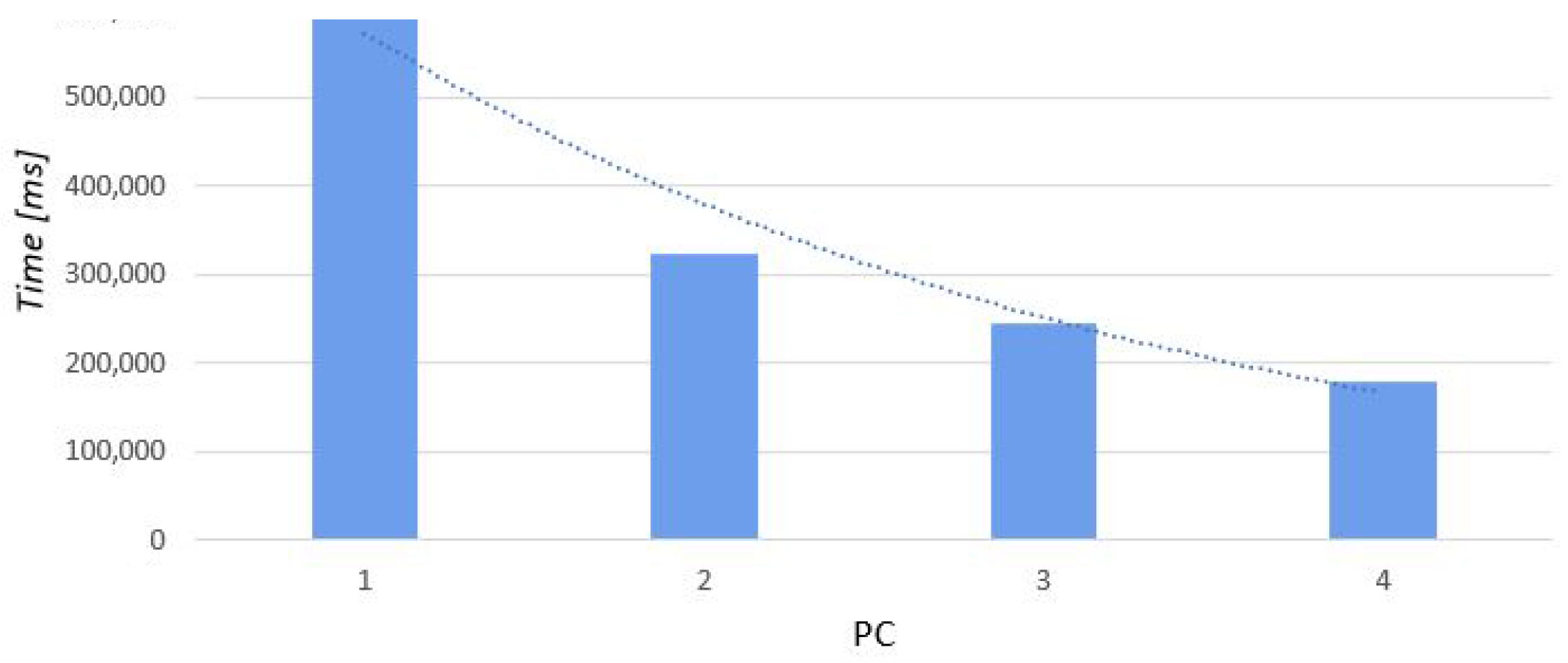
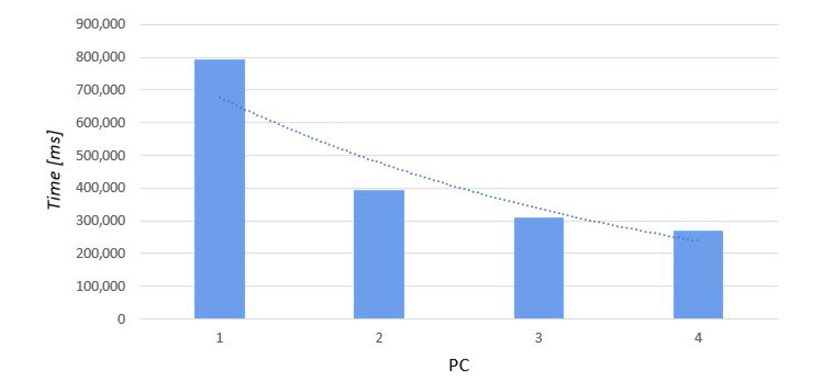
In this task, we used a point cloud that consisted of 76 × 105 points. Below is a presentation of the results, with a comparison of processing the same viewshed using a different number of computers and all available cores. The tasks were processed sequentially on all computers. In this case, the overall time needed to complete the entire task became much shorter (Table 4, Figure 6).
5.2.1. Case 1: Subdivision into 10 Parts
The table presented above (Table 4) indicates dependence between the number of computers and completion time. It shows that with the increase in the number of computers, time decreases.
5.2.2. Subdivision into Sixteen Parts
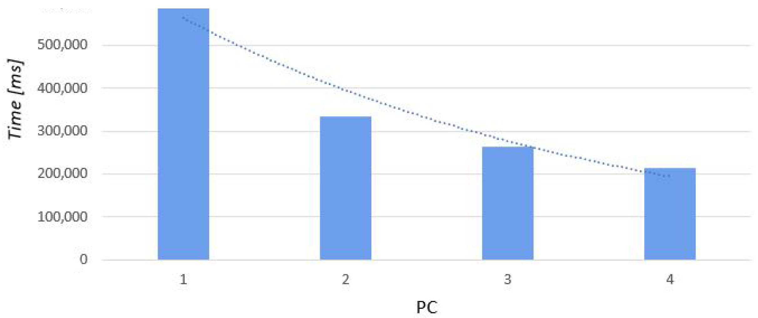
Two conclusions can be drawn from the diagrams (Figure 6 and Figure 7) and tables (Table 4 and Table 5) presented above. First, it can be concluded that increasing the number of computers on which the tasks are actually processed is justified. However, when the number of subdivisions is too large, this time cannot be effectively shortened. In the case of ten parts, the completion time was shorter than in the case of sixteen parts. This is caused by the fact that every time the program is run, the task completion time increases, which means the more instances of running the program on one computer, the longer the time required. The number of subdivisions was shown to be an important factor, affecting task completion time. It should be selected in such a way that the surface produced as a result of the subdivision has to be as large as possible, but it cannot exceed the computing capacity of the computer, and the number of divisions should be a multiple of the number of computers available.
Below is a presentation of cloud B and its respective viewsheds (Figure 8a,b).
5.3. Subdivision of Point Cloud (C) into Ten and Sixteen Parts
In the task presented here, we used a point cloud that consisted of 27 × 10 points. Below we shall present a table that compares the completion times for the same viewshed while using a different number of computers assuming the use of all available cores. The tasks were performed sequentially on each computer. As presented in the table below, the completion time of the entire task decreased substantially as the number of computers increased. (Table 6, Figure 9).
The table presented above (Table 6) indicates that task (Figure 10). completion time decreased as the number of computers increased.
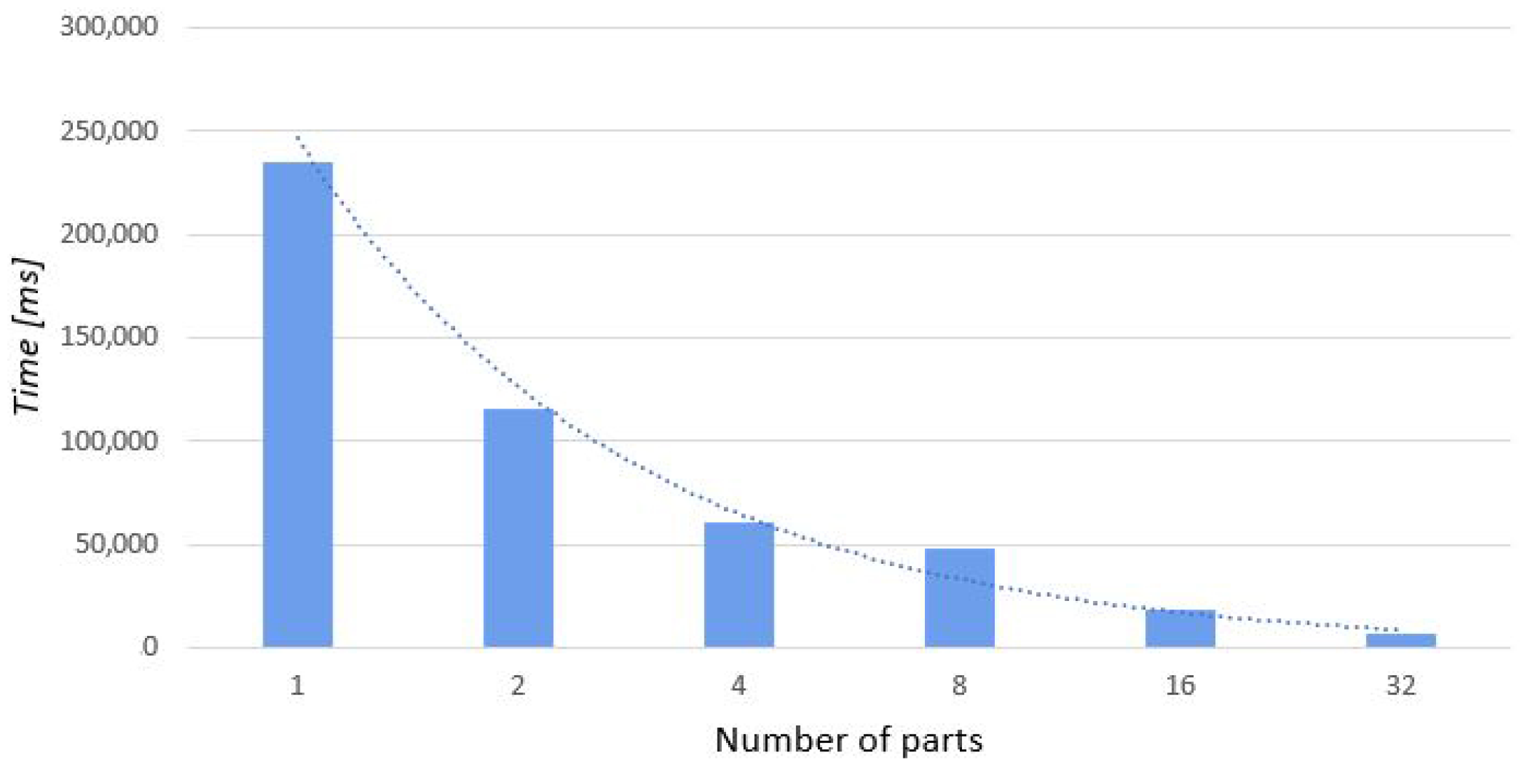
The division of the point cloud into radial sections is a process that is constant for any number of computers. It is performed on a single computer, which makes its parallelization across multiple machines unachievable. It is a bottleneck for the entire algorithm. In the stage to follow, we plan to parallelize it on a single computer using multi-threading. A table that presents division time depending on the number of parts has been presented below (Figure 11).
One major reason for the need to divide tasks across multiple machines is the necessity to load the entire point cloud into random-access memory (RAM). A subdivided point cloud occupies less space, which allows less powerful machines to process it. At present, it is impossible to determine the percentage share of points in a given point cloud subsection. This is a result of the constant angular radius that can cover a varying number of points. In the future, we plan to create an algorithm that will be able to divide point clouds following variable angular radii so as to ensure a constant point count per section. At present, RAM amount is implied by the largest cloud subsection. In addition, the size of the point cloud determines computer processing power necessary to successfully create a TIN surface.
Below is a graph that represents the dependency between the number of sections and the required amount of RAM (Figure 12). It is a simplified case in which the number of points per section is constant
The graph shown above shows that RAM demand drops as section count increases. In reference to the data presented, the most optimal division of a 64 GB cloud for a standard user is into eight sections, which results in a RAM demand of 8 GB. This is an amount that most currently available computers have at their disposal. We also leave enough free memory for other system operations to run in the background. Unfortunately, the current algorithm version cannot be directly referred to the graph above, as the number of points per section is variable, as already noted.
The time of task transfer between computers is not constant (Figure 13). Both here and in other aspects, it is a result of the variable number of points in each section. Program run time is affected only by the transfer time of a number of initial sections, which is associated with the number of node computers. Only the transfer of the initial point cloud sections is performed prior to the algorithm’s execution on node computers. The remaining clouds are transferred in parallel as the program is executed. Another factor that affects transfer time is the available bandwidth.
As shown in the graph above, transfer time shortens depending on computer count. This is due to the transfer of larger sections prior to the algorithm’s execution on node computers, which extends the overall processing time. In the case of transferring smaller sections at the start, the overall time decreases. Subsequent parts are sent during the processing of sections that have already been sent, which does not extend overall processing time.
The graph below shows the number of points in a section depending on section count (Figure 14). It can be seen that as the number of sections grows, the number of points decreases. However, in this case we have also accounted for an even division, in which each section is of equal size. In the case of the algorithm presented, we can encounter a situation in which there is a division into four sections and one of them can be even a dozen or so times larger than the other sections. This depends on the location of the division point within the cloud.
Below is a presentation of two divisions of a single cloud with a point count of 15 × 10 into four sections, but from different points (Figure 15a,b).
The maximum point count in the first division is 380,113 while in the second it is 586,923.
Unfortunately, it is impossible to identify the mode of division, as it primarily depends on the location of the central division point relative to the entire cloud.
The principle that should be followed in selecting the number of computers and sections is to ensure a division in which the largest section can fit into a computer’s RAM and the number of computers is equal to the number of sections. Unfortunately, it is very rare for this to be the case. When dealing with a substantial number of sections, we should strive to arrive at a division in which the maximum section size can fit into a computer’s memory while keeping the number of sections as low as possible. In this distribution, the number of points from the cloud allocated to each computer can differ up to several times. We are of the opinion that we should assume the worst case scenario, in which there is a single part that is substantially larger. All computers must have the parameters necessary to process this cloud. Our future research is aimed at creating an algorithm that would divide point clouds into radial sections while accounting for a variable angular radius so as to keep the number of points per section constant.
6. Other Uses of the Algorithm
The method of parallelization of computations presented in this article can be used in many engineering fields. Even with minor changes, they do not have to be related to the point cloud. In fact, any more complex task can be broken down into smaller ones and distributed among multiple computers. An example of such tasks may be calculations on multidimensional tables, where their respective parts are sent to different computers, analyses of the strength of building components where another computer is responsible for each group of elements, or even the simple studies of the impact of variable coefficients on the environment, where each change is computed by a different computer. There are many possibilities, but they require adjustments and slight changes to the algorithm and the entire program.
7. Other Studies
The authors of other studies mostly focused on parallelizing the first operation type, namely processing the entire point cloud [23,24], for instance with the aim of dividing it. Here, parallelization is based on dividing points between a processor’s cores and threads (reference). We have also studied this. In this paper, we have not focused on parallelizing the point cloud division itself, but on parallelizing the task of creating TIN surfaces on them and generating viewsheds. Simplifying the triangulation of the entire point cloud via its division and transfer to multiple computers lowers processing power and RAM demand. It also shortens processing and in some cases enables this processing altogether. A similar algorithm has been applied in 3dsMax ® [25], but it is not associated with triangulation, but with rendering individual animation frames.
Unfortunately, at present there is no algorithm that could solve the task presented. Comparing the parallelization of a different part of the algorithm with parallelizing task transfer would bring neither desirable nor comparable outcomes.
8. Validation
The presented results indicate what should be the appropriate procedure for dividing a task and distributing individual subtasks into computing resources. The calculation times and hardware conditions quoted here allow to select the appropriate division and distribution strategy depending on whether the calculation is a single viewshed or a visibility map consisting of many graphs. It can be seen that splitting a single viewshed job and distributing these parts to 2 computers allows you to get the result faster than on one machine, despite time consuming distribution. The time gain is also noticeable when distributing tasks to separate processes assigned to single processors on one computer. Running consecutive parts of the task in parallel on 4 cores resulted in almost three times faster than calculating these parts one after another on 4 cores. It follows that performing these calculations in parallel, both on one computer and on several computers, is always profitable.
9. Discussion
The comparison of calculation times presented in Section 5 clearly indicates that when a single computer is used, the number of processors engaged in the calculations significantly affects the algorithm execution time. In the tasks presented, both in the case of executing the process sequentially and in parallel, the time required decreased significantly. This proves that poor processor core management can lead to ineffective computer work and to wastage of computing power at our disposal. In the case of more advanced tasks, distributing them to node computers also brought the expected results, i.e., a decrease in completion time. The results point to an important conclusion that the appropriate selection of point cloud subdivision parts is essential. Should this selection be inappropriate, completion time will not be effectively decreased. The parts produced via subdivision should be selected in such a manner as to make maximum use of a computer’s computing power. Their number should be a multiple of the number of available computers. Only then can we effectively accelerate the process.
10. Conclusions
The time decreases obtained with different acceleration methods presented here can be compared. With the use of multiple computers, a single computer, a multi-threaded processor or the use of the graphics card’s computing power. Every solution that speeds up the process is good, but users might not necessarily be able to use each one. Not everyone has a dedicated graphics card, multi-core processor or access to several computers. When developing software, we need to keep in mind who is going to use it and what possibilities they will have in terms of running it. The best solution, as in the case presented, is to develop software dedicated to a specific user. Likewise, we should adapt the acceleration method to the algorithm in use. Not every program can be parallelized using every type of technology. The best solution is to use all solutions available on both the programming and hardware side.
The paper clearly demonstrates a significant acceleration of calculations executed to solve a specific engineering problem. The method proposed allows engineers to make good use of well-known software, which allows complete supervision and control of the process and its output. Another advantage is the possibility of using available hardware outside of the hours when it is in direct use. This method is an example in which engineers have the ability to process large datasets in a productive and creative manner, suitable to their needs.
Author Contributions
Conceptualization, J.O. and P.O.; methodology, J.O. and P.O.; software, J.O. and P.O.; validation, J.O. and P.O.; formal analysis, J.O. and P.O.; investigation, J.O. and P.O.; resources, J.O. and P.O.; data curation, J.O. and P.O.; writing—original draft preparation, J.O. and P.O.; writing—review and editing, J.O. and P.O.; visualization, J.O. and P.O.; supervision, J.O. and P.O.; project administration, J.O. and P.O.; All authors have read and agreed to the published version of the manuscript.
Funding
This research received no external funding.
Institutional Review Board Statement
Not applicable.
Informed Consent Statement
Informed consent was obtained from all subjects involved in the study.
Data Availability Statement
Not applicable.
Acknowledgments
The author would like to express their thanks to the editors for their helpful comments in advance.
Conflicts of Interest
The authors declare no conflict of interest.
References
- Valeriy, Y.; Mallet, C.; David, N. Catchment hydrologic response with a fully distributed triangulated irregular network model. Water Resour. Res. 2004. [Google Scholar] [CrossRef]
- Kurczyński, Z. Forogramertia; Wydawnictwo Naukowe PWN: Warsaw, Poland, 2014. [Google Scholar]
- Ptak, A. LiDAR w wielkim mieście. Geodeta Magazyn Geoinformacyjny 2014, 12, 28–29. [Google Scholar]
- Orlof, J. Chmura punktów—Nowa struktura danych. Aura Ochrona Środowiska 2017, 12, 3–6. [Google Scholar]
- LAS (LASer) File Format, Version. Library of Congress. 2015. Available online: https://www.loc.gov/preservation/digital/formats/fdd/fdd000418.shtml (accessed on 12 September 2020).
- Orlof, J.; Ozimek, P.; Łabędź, P.; Widłak, A.; Nytko, M. Determination of Radial Segmentation of Point Clouds Using K-D Trees with the Algorithm Rejecting Subtrees. Symmetry 2019, 11, 1451. [Google Scholar] [CrossRef] [Green Version]
- Martin, R.C. Clean Architecture: A Craftsman’s Guide to Software Structure and Design; Pearson Education: London, UK, 2017. [Google Scholar]
- Pllana, S.; Xhafa, F. Programming Multi-Core and Many-Core Computing Systems; Wiley: Hoboken, NJ, USA, 2017. [Google Scholar]
- Chandra, R.; Dagum, L.; Kohr, D.; Maydan, D.; McDonald, J.; Menon, R. Parallel Programming in Openmp; Morgan Kaufmann: Burlington, MA, USA, 2001. [Google Scholar]
- Chapman, B.; Jost, G.; Van Der Pas, R. Using OpenMP: Portable Shared Memory Parallel Programming; MIT Press: Cambridge, MA, USA, 2008. [Google Scholar]
- Pacheco, P. Parallel Programming with MPI; Morgan Kaufmann: Burlington, MA, USA, 1996. [Google Scholar]
- Wen-mei, W. GPU Computing Gems Emerald; Morgan Kaufmann: Burlington, MA, USA, 2011. [Google Scholar]
- Xi, W.; Zhou, X.; Zhang, J. An upgraded visualization and analytical tool for landscape modeling. Environ. Model. Softw. 2020, 134, 104849. [Google Scholar] [CrossRef]
- Risse, B.; Mangan, M.; Sturzl, W.; Webb, B. Software to convert terrestrial LiDAR scans of natural environments into photorealistic meshes. Environ. Model. Softw. 2018, 99, 88–100. [Google Scholar] [CrossRef] [Green Version]
- Fagerman, J.; Juchmann, W. Lidar Scanning by Helicopter in the USA. 2015. Available online: https://www.gim-international.com/content/article/lidar-scanning-by-helicopter-in-the-usa (accessed on 12 November 2020).
- Han, X.F.; Jin, J.S.; Wang, M.J.; Jiang, W.; Gao, L.; Xiao, L. A review of algorithms for filtering the 3D point cloud. Signal Process. Image Commun. 2017, 57, 103–112. [Google Scholar] [CrossRef]
- Informatyczny System Osłony Kraju. 2012. Available online: http://www.isok.gov.pl/en/about-the-project (accessed on 10 November 2020).
- Orlof, J. Point Cloud based viewshed generation in Autocad Civil 3D. Tech. Trans. 2017, 12, 143–155. [Google Scholar]
- Tickoo, S. Exploring AutoCAD Civil 3D 2017; Cadcim Technologies: Schererville, IN, USA, 2016. [Google Scholar]
- Allain, A. Jumping into C++; Cprogramming.com: Somerville, MA, USA, 2013. [Google Scholar]
- White, M. Mastering C#; Independently published: Traverse City, MI, USA, 2019. [Google Scholar]
- Muntasir, K.; Tickoo, S. Batch File: The Resource Guide to Batch File Code and Commands; CreateSpace Independent Publishing Platform: Scotts Valley, CA, USA, 2011. [Google Scholar]
- Najdataei, H.; Nikolakopoulos, Y.; Gulisano, V.; Papatriantafilou, M. Continuous and Parallel LiDAR Point-Cloud Clusterin. In Proceedings of the 2018 IEEE 38th International Conference on Distributed Computing Systems (ICDCS), Vienna, Austria, 2–6 July 2018; pp. 671–684. [Google Scholar] [CrossRef]
- Zeng, X.; He, W. GPGPU-based parallel processing of massive LiDAR point cloud. Proc. SPIE 2009. [Google Scholar] [CrossRef]
- Mahmoud, A.; ALmurshidi, H.S. Backburner Management For Network Rendering 3DS MAX. JMESS 2017, 3, 2458–2925. [Google Scholar]
Figure 1.
(a) A fragment of a city seen in orthogonal projection, with an observation point marked in red. (b) A Viewshed generated for the observation point.
Figure 1.
(a) A fragment of a city seen in orthogonal projection, with an observation point marked in red. (b) A Viewshed generated for the observation point.

Figure 2.
A Viewshed creation block diagram.

Figure 3.
The principle of task distribution across numerous computers.

Figure 4.
The program operation block diagram.

Figure 5.
(a) A point cloud (A). (b) The final viewshed for task 1, point cloud (A).

Figure 6.
Dependence between the number of computers and completion time.

Figure 7.
Dependence between the number of PCs and calculation completion time for cloud (B), divided into 16 parts.
Figure 7.
Dependence between the number of PCs and calculation completion time for cloud (B), divided into 16 parts.

Figure 8.
(a) A point cloud (B). (b) The final viewshed for task 2, point cloud (B).

Figure 9.
Dependence between the number of PCs and time of calculation performed on point cloud (C), divided into 16 parts.
Figure 9.
Dependence between the number of PCs and time of calculation performed on point cloud (C), divided into 16 parts.

Figure 10.
The final viewshed point cloud (C).

Figure 11.
Dependence between the number of parts and divide time.

Figure 12.
Dependence between the number of parts and RAM (random-access memory).

Figure 13.
Dependence between the number of parts time transfer.

Figure 14.
Dependence between the number of parts and points in part.

Figure 15.
(a) A fragment of a point cloud divided in four parts. (b) A fragment of a point cloud divided in four parts.
Figure 15.
(a) A fragment of a point cloud divided in four parts. (b) A fragment of a point cloud divided in four parts.


Table 1.
Task 1 performance time, performed sequentially on cloud point (A) on a single computer with the use of different numbers of processor cores.
Table 1.
Task 1 performance time, performed sequentially on cloud point (A) on a single computer with the use of different numbers of processor cores.
| Core | 1 | 2 | 4 |
|---|---|---|---|
| Time [ms] | 1,129,225 | 612,482 | 602,478 |
Table 2.
Task 1 performance time, performed on point cloud (A), on a single computer with the parallel use of varying number of processor cores.
Table 2.
Task 1 performance time, performed on point cloud (A), on a single computer with the parallel use of varying number of processor cores.
| Core | 1 | 2 | 4 |
|---|---|---|---|
| Time [ms] | 792,035 | 379,278 | 204,832 |
Table 3.
Comparison of the time necessary to process a single part of cloud (A) on one core with the processing time of four parts of cloud (A) on four cores in parallel.
Table 3.
Comparison of the time necessary to process a single part of cloud (A) on one core with the processing time of four parts of cloud (A) on four cores in parallel.
| Cloud Parts/Core | 1/1 | 4/4 |
|---|---|---|
| Time [ms] | 199,275 | 202,868 |
Table 4.
Completion time of task 2, performed on point cloud (B), sequentially, on different numbers of computers.
Table 4.
Completion time of task 2, performed on point cloud (B), sequentially, on different numbers of computers.
| PC | 1 | 2 | 3 | 4 |
|---|---|---|---|---|
| Time [ms] | 641,035 | 324,583 | 245,481 | 178,425 |
Table 5.
Completion time of task 2, performed on point cloud (B), in parallel, on a different number of computers.
Table 5.
Completion time of task 2, performed on point cloud (B), in parallel, on a different number of computers.
| PC | 1 | 2 | 3 | 4 |
|---|---|---|---|---|
| Time [ms] | 641,035 | 333,861 | 262,800 | 212,968 |
Table 6.
Performance time of task 2, on point cloud (C), in parallel, on a different number of computers that operated sequentially.
Table 6.
Performance time of task 2, on point cloud (C), in parallel, on a different number of computers that operated sequentially.
| PC | 1 | 2 | 3 | 4 |
|---|---|---|---|---|
| Time [ms] | 792,584 | 394,626 | 310,788 | 268,859 |
Publisher’s Note: MDPI stays neutral with regard to jurisdictional claims in published maps and institutional affiliations. |
© 2021 by the authors. Licensee MDPI, Basel, Switzerland. This article is an open access article distributed under the terms and conditions of the Creative Commons Attribution (CC BY) license (http://creativecommons.org/licenses/by/4.0/).
Share and Cite
MDPI and ACS Style
Orlof, J.; Ozimek, P. TIN Surface and Radial Viewshed Determination Algorithm Parallelisation on Multiple Computing Machines. Symmetry 2021, 13, 424. https://0-doi-org.brum.beds.ac.uk/10.3390/sym13030424
AMA Style
Orlof J, Ozimek P. TIN Surface and Radial Viewshed Determination Algorithm Parallelisation on Multiple Computing Machines. Symmetry. 2021; 13(3):424. https://0-doi-org.brum.beds.ac.uk/10.3390/sym13030424
Chicago/Turabian StyleOrlof, Jerzy, and Paweł Ozimek. 2021. "TIN Surface and Radial Viewshed Determination Algorithm Parallelisation on Multiple Computing Machines" Symmetry 13, no. 3: 424. https://0-doi-org.brum.beds.ac.uk/10.3390/sym13030424
Note that from the first issue of 2016, this journal uses article numbers instead of page numbers. See further details here.