
Chaotic Compressive Spectrum Sensing Based on Chebyshev Map for Cognitive Radio Networks


1
RITM Laboratory, CED Engineering Sciences, Hassan II University, Casablanca 20000, Morocco
2
Department of Electrical and Computer Engineering, The University of North Carolina at Charlotte, Charlotte, NC 28223, USA
*
Authors to whom correspondence should be addressed.
Symmetry 2021, 13(3), 429; https://0-doi-org.brum.beds.ac.uk/10.3390/sym13030429
Submission received: 8 February 2021
/
Revised: 27 February 2021
/
Accepted: 2 March 2021
/
Published: 7 March 2021
Abstract
:Recently, the chaotic compressive sensing paradigm has been widely used in many areas, due to its ability to reduce data acquisition time with high security. For cognitive radio networks (CRNs), this mechanism aims at detecting the spectrum holes based on few measurements taken from the original sparse signal. To ensure a high performance of the acquisition and recovery process, the choice of a suitable sensing matrix and the appropriate recovery algorithm should be done carefully. In this paper, a new chaotic compressive spectrum sensing (CSS) solution is proposed for cooperative CRNs based on the Chebyshev sensing matrix and the Bayesian recovery via Laplace prior. The chaotic sensing matrix is used first to acquire and compress the high-dimensional signal, which can be an interesting topic to be published in symmetry journal, especially in the data-compression subsection. Moreover, this type of matrix provides reliable and secure spectrum detection as opposed to random sensing matrix, since any small change in the initial parameters generates a different sensing matrix. For the recovery process, unlike the convex and greedy algorithms, Bayesian models are fast, require less measurement, and deal with uncertainty. Numerical simulations prove that the proposed combination is highly efficient, since the Bayesian algorithm with the Chebyshev sensing matrix provides superior performances, with compressive measurements. Technically, this number can be reduced to 20% of the length and still provides a substantial performance.
1. Introduction
The cognitive radio system has been proposed as a convenient solution to enhance the radio spectrum utilization and deal with spectrum scarcity issue in the next generation of wireless communications. It allows secondary/unlicensed users (SUs) to intelligently identify vacant primary communication channels, called spectrum holes, to use them for data transmission, without any interferences with primary/licensed users (PUs) [1,2]. In this respect, spectrum sensing is the main component in cognitive radio cycle since it is the process in which the measurements are performed. Due to several wireless transmission impairments, such as noise, multipath fading, and other varying environmental conditions, this process can be affected by the uncertainty in measurements, which decreases the cognitive radio performance [3]. To enhance the sensing results, SUs can cooperate with each other by exchanging sensing data, to get a relevant decision about the spectrum occupancy.
Cooperative spectrum sensing is conceived to improve the sensing performance and decision reliability by analyzing the current connections between different SUs monitoring the same spectrum. In the literature, cooperative sensing architecture can be divided into three main schemes: centralized [4], distributed [5], and external [6]. In the centralized scheme, SUs report their sensing information to a fusion center, which collects all sensing results to make an appropriate decision on spectrum occupancy. On the contrary, in the distributed scheme, the spectrum sensing is performed independently by SUs without the fusion center intervening. While in the external structure, the sensing decision is taken by an external device, which applies technical limitations on the SUs through the sensing process.
The network functionalities based on the above methods can be disrupted when unauthorized users attempt to access the system. As a result, several challenges need to be addressed, including the authentication of SUs belonging to the same network, the confidentiality of the sensing information, the sensing measurements uncertainty, and sensing time. Therefore, the design of an efficient cooperative sensing network is dependent on three aspects: securing communication links between the different nodes and the fusion center of the network [7,8], dealing with uncertainty in measurements, and accelerating the spectrum sensing. To address these different concerns, many solutions using the compressive sensing technique, are proposed in the literature.
Compressive sensing was first proposed by Candès et al., as a new paradigm to achieve a signal-sampling rate under the traditional Shannon–Nyquist one [9]. This technique can successfully restore the original signal from just a few linear measurements. To sense wideband spectrum in CRNs, Tian and Giannakis introduced the theory of compressive spectrum sensing (CSS), which combines the compressive sensing technique with the spectrum sensing process [10]. Then, the concept of CSS was extended and implemented for cooperative CRNs by Tian [11]. Subsequently, several solutions have been proposed in this field from different perspectives based on three common processes: sub-Nyquist sampling, sparse recovery, and spectrum detection [12]. The first process aims at presenting the original signal in a suitable sparse basis, to be compressed then by the sensing matrix and reducing its dimension consequently. Next, the sparse signal is recovered from the few linear measurements taken in the first step. At last, the spectrum sensing process is performed based on different sensing techniques such as energy detection [13], Autocorrelation detection [14], matched filter detection [15], machine learning [16], wavelet detection [17], and blind spectrum detection [18].
For the sub-Nyquist sampling process, the design of the sensing matrix is the key of a successful compressive sensing solution. Random matrices [19] are the most widely used as sensing matrices due to their theoretical benefits as to universality and construction ease. Examples of these matrices include Gaussian, Bernoulli, Hadamard, and uniform matrices. Despite their advantages, hardware implementation of random matrices is costly and requires a large storage memory, which makes the use of this type of matrices impractical for some large-scale applications. To address these limitations, deterministic matrices [20] are developed as an alternative solution. These matrices achieve the same performance as random matrices but with less computational complexity, reduced memory usage and fast recovery. Examples of deterministic matrices include Toeplitz [21], Circulant [22], and Binary BCH. In this paper, we focus on other attractive types of sensing matrices for compressive sensing called chaotic sensing matrices. This category of matrices provides the advantages of both random and deterministic matrices. Chaotic system produces a pseudo-random matrix in a deterministic approach, which can improve the efficiency of the system. Another interesting benefit of chaotic sensing matrices is security, since joining the network by an external user requires knowledge of the initial conditions used for producing the sensing matrix; otherwise, the user can be rejected by the network and identified as a hacker. There are several maps to generate chaotic matrices, including the logistic map [23], quadratic map [24], Chebyshev map [25], tent map [26], and many other types.
For the sparse recovery process, several algorithms have been proposed to estimate a sparse signal with a lower number of compressed measurements. The aim of these algorithms is finding the sparest solution of the undetermined system presenting the acquisition operation. In the literature, the recovery algorithms are classified under three approaches: convex optimization [27], greedy [28], and Bayesian models [29]. The convex optimization algorithms rely on linear programming to solve the compressive sensing recovery problems. Some examples of algorithms under this approach are basis pursuit (BP; also called l1 minimization) and gradient descent. The greedy approach is an iterative method for estimating the sparse signal coefficients by looking for a local optimal at each iteration. Examples of greedy algorithms include matching pursuit, orthogonal matching pursuit (OMP), and subspace pursuit. Bayesian model is a statistical method that defines the input signal through probability distributions to deal with uncertainty in measurements, which makes it different from previous approaches that consider deterministic signal input. Examples of Bayesian recovery algorithms include Laplace priors, belief propagation, and relevance vector machine. However, convex algorithms are robust to noise but slower, uncertain, and difficult to implement for large-size applications. Greedy algorithms are fast but uncertain and require more measurements than convex algorithms. Bayesian models possess the benefits of both categories. They are fast, require less measurement, and deal with uncertainty.
Since chaotic sensing matrices were proposed to compressive sensing [30], various modifications and enhancements have been applied to improve this type of matrices. For instance, the authors in Reference [31] performed an experimental analysis to prove that the chaotic sensing matrices based on the two sequences Chua and Lorenz provide the same performance results as those using random sensing matrices. Moreover, Gan et al. presented a new chaotic construction based on Chebyshev sequence, which has a good sampling efficiency for sparse signals [25]. Few years later, a generalization of the previous method has been developed and published in Reference [32] for topologically conjugate chaotic systems. Most recently, the authors in Reference [33] used a chaining method to construct a novel sinusoidal chaotic sensing matrix with no transient time for compressive sensing. Furthermore, many structural chaotic sensing matrices have also been proposed for some particular applications of compressive sensing [34,35,36]. For Example, the authors in Reference [34] presented a Toeplitzed structurally chaotic matrix, using two steps. In the first step, they multiplied an orthonormal matrix with a chaotic-based Toeplitz matrix. In the second step, they subsampled the resultant matrix to obtain the structural one. In Reference [35], the authors generated an incoherence rotated chaotic matrix based on QR decomposition. They choose first an appropriate chaotic system and remove the first 1000 chaotic elements. Then, the first row of the sensing matrix is fixed and the remaining rows are generated by a circular way. In Reference [36], the authors developed an inversion operator, a chaotic-based circulant matrix, and a subsampling operator, to construct a new structural chaotic sensing matrix, based on the chaotic Chebyshev map.
Much progress has been achieved by using chaotic sensing matrices in real-world applications. For instance, Kamel et al. proposed a new technique to fill up a chaotic sensing matrix for CSS in CRNs [37]. The authors used different initial parameters for every column of the sensing matrix, to improve the randomness of the matrix and provide inherent security to the compressive sensing system. Examples of more applications of chaotic matrices are image encryption [38], body-to-body networks [39], network coding [40], and wireless sensor networks [41]. However, all the work already mentioned focuses mainly on the sub-sampling process of the compressive sensing technique. For the signal recovery process, they commonly use convex or greedy algorithms with more complexity and do not deal with uncertainty in measurements. Indeed, to our best knowledge, a few papers use chaotic sensing matrices in CRNs. Therefore, designing a comprehensive and efficient cognitive radio system that supports the improvement in the two main processes of compressive sensing is still a topic that deserves to be studied and which can be an attractive subject for computer science, theory, and methods of symmetry journals.
In this paper, we present a novel CSS solution for CRNs. The proposed technique is based on a robust combination that exploits the efficiency of Bayesian recovery via Laplace prior algorithm and the strengths of chaotic sensing matrix, using Chebyshev map. Compared to the existing techniques, our proposed model is a trade-off to improve the performance of CSS technique in CRNs by addressing three main challenges at once. The first one is dealing with the uncertainty issue in measurements by using Bayesian inference, which is a powerful probabilistic method. This technique uses patterns inside prior data to predict future events. The second challenge is accelerating the spectrum sensing process by using the compressive sensing technique, which acquires a high-dimensional signal with a lower number of measurements and less processing time, as well. The third challenge is providing comprehensive security to the system by using Chebyshev sensing matrix, since any small change in the initial parameters generates a different sensing matrix. This means that it is very difficult for an external user to use the network without having prior information about the initial parameters used to generate the sensing matrix.
The main contributions of this work are summarized as follows:
- Review of the compressive sensing theory;
- Review of the cooperative spectrum sensing theory;
- Analysis of Chebyshev sensing matrix;
- Mathematical model of the Bayesian recovery;
- Performance Evaluation of the proposed technique based on different metrics;
- Comparison between Chebyshev matrix and logistic, quadratic, and random matrices.
The rest of this paper is structured in three main sections: Section 2 reviews the theoretical background about compressive sensing and spectrum sensing. Section 3 presents the system model and the methodology of the proposed technique. Section 4 analyzes the experiments results of the proposed technique, using different metrics. Last, a conclusion is given.
2. Literature Review
2.1. Compressive Sensing Model
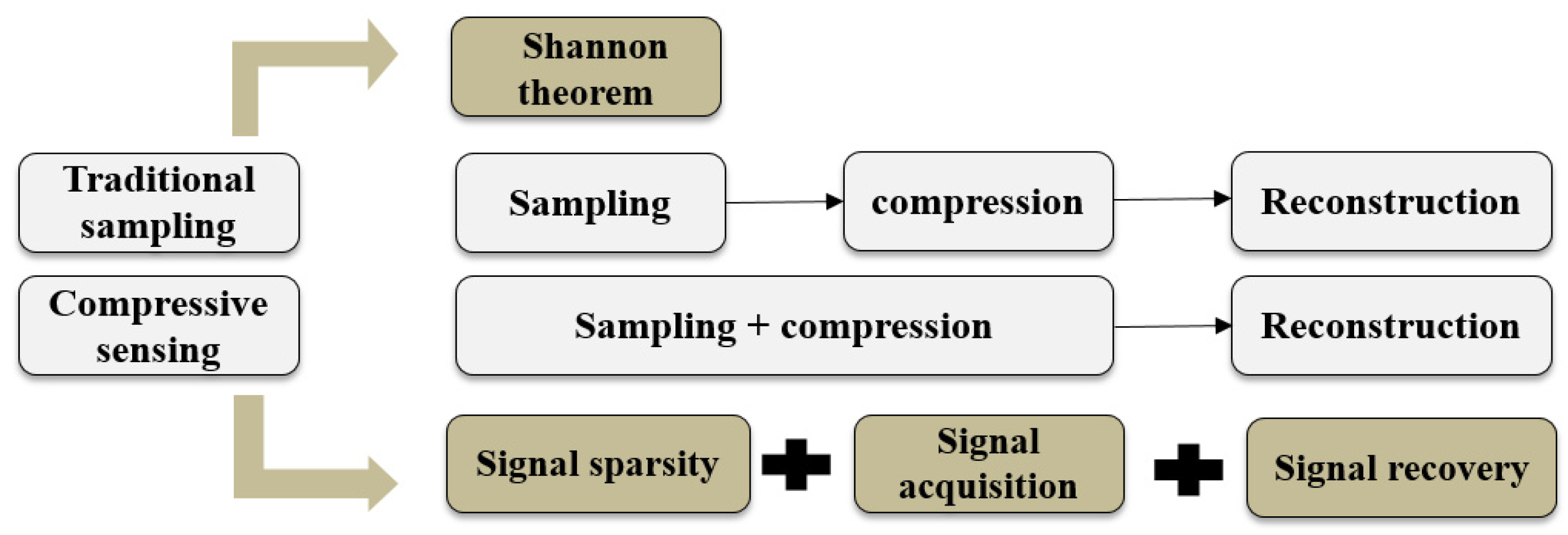
Compressive sensing is a powerful technique, which combines both, sampling and compression technologies in a one-step process. It is firstly presented as innovative method to sample signals with a lower frequency than Shannon’s one, to accelerate the channels sensing, minimize the complexity of the computations and decrease the hardware cost [42,43]. The reduction of hardware cost occurs by using different schemes to replace the classical ADC used at the Nyquist rate. These schemes decrease the number of samples required for high-dimensional-signal acquisition while consuming less energy. For examples, the authors in Reference [44] proposed a new scheme of compressive sensing technique to increase the battery lifetime of the sensor nodes during transmission. In Reference [45], the authors proposed a novel design for deterministic compressive sensing recovery that consumes less power and hardware resources (less DSP cores and RAM). In References [46,47], the authors studied one-bit compressive sensing as a suitable solution to decrease the hardware cost by considering only the sign of every measurement. Figure 1 illustrates the three major processes involved in the compressive sensing concept: signal sparsity, signal acquisition, and signal recovery.
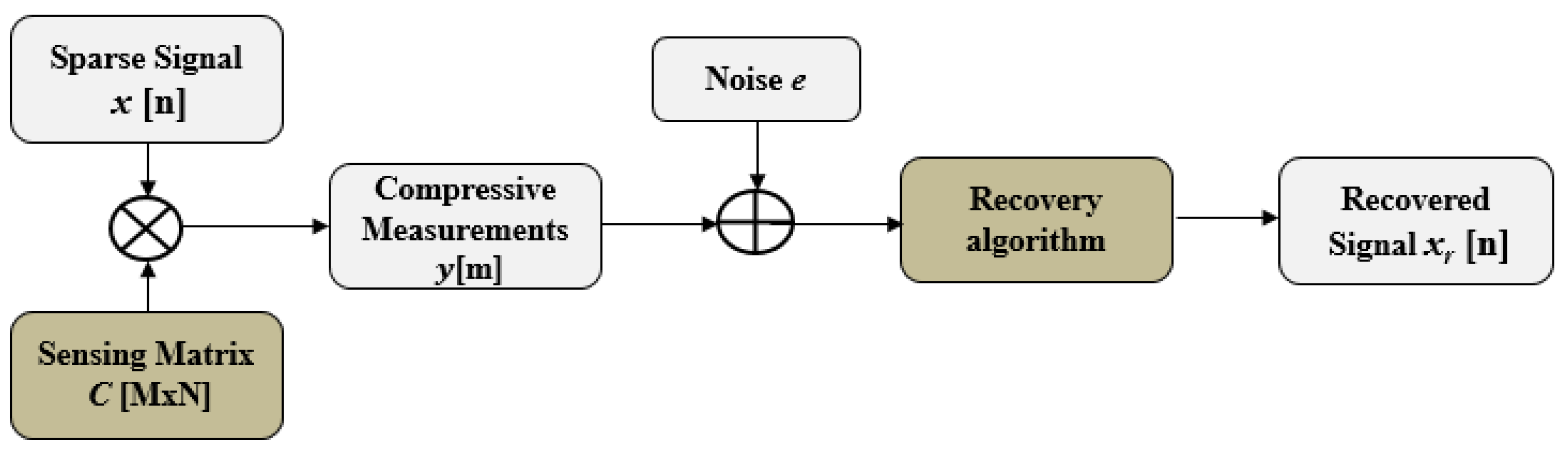
Let x ∈ RN be a K-sparse signal of length n in a specific dictionary D; thus, x can be approximated by sparse vector, q, which contains, at most, K non-zeros, and (N − k) entries are zero, i.e., x = Dq and ∥q∥0 ≤ K. Then, the compression process is represented as a result of the multiplication operation of a sensing matrix C and the sparse signal x. It can be described mathematically, as follows:
where C ∈ RM×N is a M × N sensing matrix, y ∈ RM is the compressive measurement vector of length m << n, and e is the measurement noise. Figure 2 represents the general model of compressive sensing.
y = Cx + e
To determine the optimal and sparsest solution of the underdetermined system given by (1), the sensing matrix C must be appropriately selected. Many requirements of sensing matrix C are discussed in the literature, to guarantee a robust and stable signal reconstruction, most commonly used in theory the restricted isometry property (RIP) [48] and the mutual coherence [49]. For the RIP, it is a feature of orthonormal matrices related to a restricted isometric constant. A matrix C ∈ RM×N that satisfies the RIP in order k is given by the following equation:
where ε is the restricted isometry constant of the sensing matrix C, is the l2-norm, and x is the received sparse signal. Random sensing matrices have been confirmed to satisfy the RIP with high probability [50]. For the coherence criterion, it evaluates the sensing matrix quality and its efficacy. The mutual coherence of a matrix is denoted as μ(C), which measures the maximal value of correlation between the columns of C. It is defined as follows:
where Ci and Cj are two normalized columns of C. Low coherence corresponds to low correlation between the columns of C, implying that a small number of compressive measurements are required for signal recovery.
μ(C) = max |<Ci|Cj>|
Then, the sparse signal, x, can be restored from the set of compressive measurements y by solving Equation (1). This operation can be formulated as l0-minimisation problem to find the optimal solution of the system as follows:
where xr is the estimate of x and is the l0-norm, which calculates the number of non-zero coefficients of a vector. In complexity theory, the l0-minimization has been qualified as NP-hard problem. Therefore, to address this complexity, a number of methods using convex optimization algorithms, are proposed as an alternative solution to solve this problem, which uses l1-norm instead l0-nom [51], as follows:
where is the l1-norm that provide the sum of elements of a vector. The compressive recovery algorithms recommended in the literature to solve this type of problems can be categorized into three approaches: convex, greedy, and Bayesian. The aim of these algorithms is finding the sparse solution of the input signal from less number of measurements and by addressing different factors including noise, complexity, and performance guarantees.
2.2. Cooperative Spectrum Sensing Model
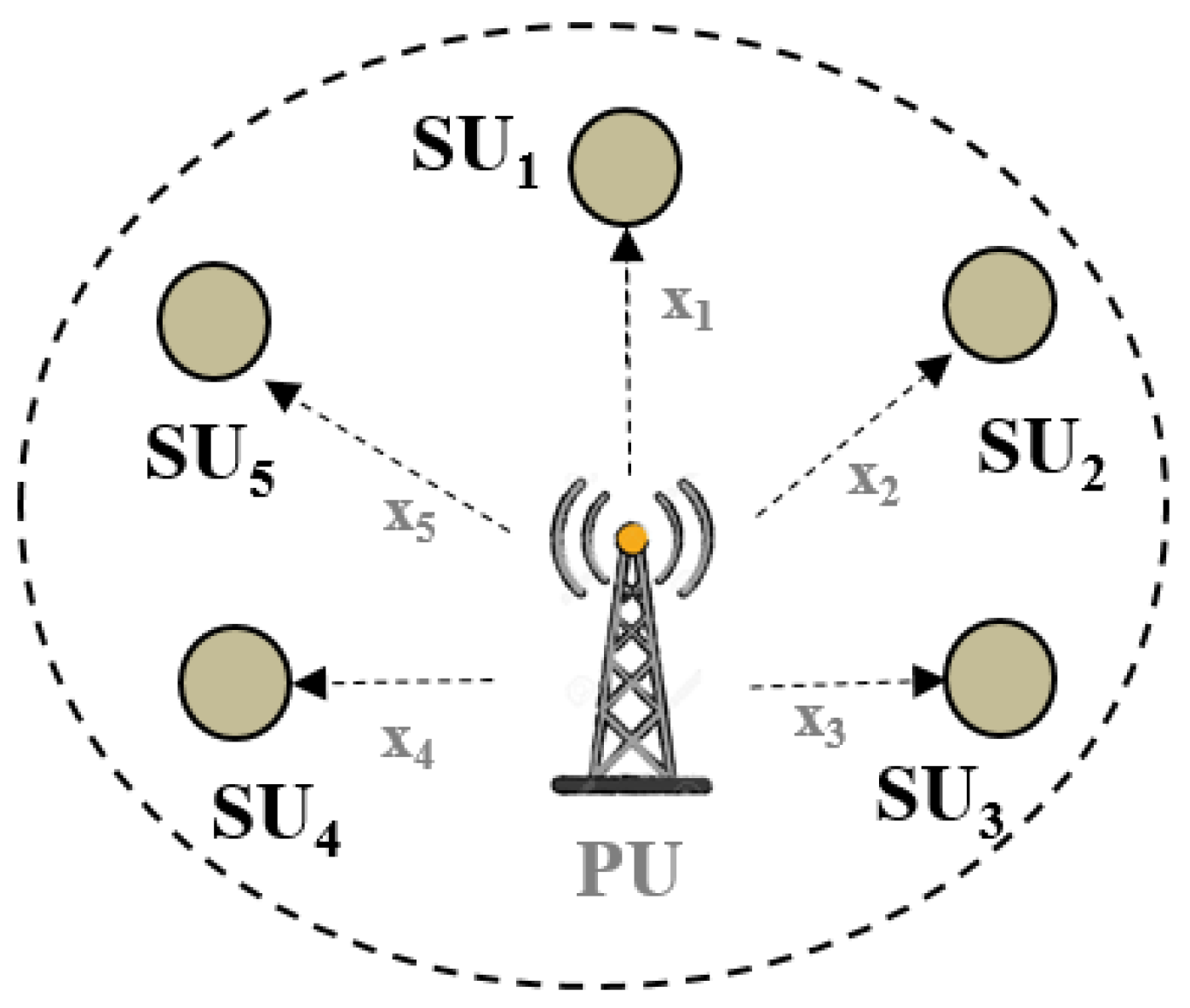
Spectrum sensing is the crucial process in the cognitive radio cycle. It allows SUs to detect the unused primary spectrum, called spectrum holes, in order to exploit them for data transmission, without any interference with PUs [52]. For cooperative sensing model [53], the received signal of the ith SU can be defined as follows:
where N is the number of samples, xi(n) is the ith SU received signal, s(n) presents the PU signal, and wi(n) is the additive white Gaussian noise (AWGN) with zero mean and variance δw. H0 and H1 denote respectively the absence and the presence of the PU signal. Figure 3 shows an example of the cooperative sensing network.
xi(n) = wi(n) H0: PU is absent
xi(n) = s(n) + wi(n) H1: PU is present
xi(n) = s(n) + wi(n) H1: PU is present
To investigate the received signal xi(n), there are several spectrum sensing techniques proposed in the literature that can be used, including energy detection, machine learning, and matched filter. Then, to make a relevant decision about the occupancy of the PU, an adaptive threshold, denoted by Λ, is selected according to sensing technique used and compared next to the output signal T of each node, as follows:
if T ≥ Λ, H1: PU is present
if T < Λ, H0: PU is absent
if T < Λ, H0: PU is absent
Subsequently, each SU achieves its local decision using the results of the comparison.
To evaluate a cooperative spectrum sensing technique, three main evaluation metrics can be used: the cooperative probability of detection, the cooperative probability of false alarm, and the cooperative probability of miss detection [53]. These probabilities are derived from the individual spectrum sensing metrics, as follows:
- The cooperative probability of detection (Cd) is defined as follows:
Cd = 1 − (1 − Pd )p
- The cooperative probability of false alarm (Cfa) is defined as follows:
Cfa = 1 − (1 − Pfa )p
- The cooperative probability of miss detection (Cmd) is defined as follows:
Cmd = 1 − (1 − Pmd )p
3. Methodology
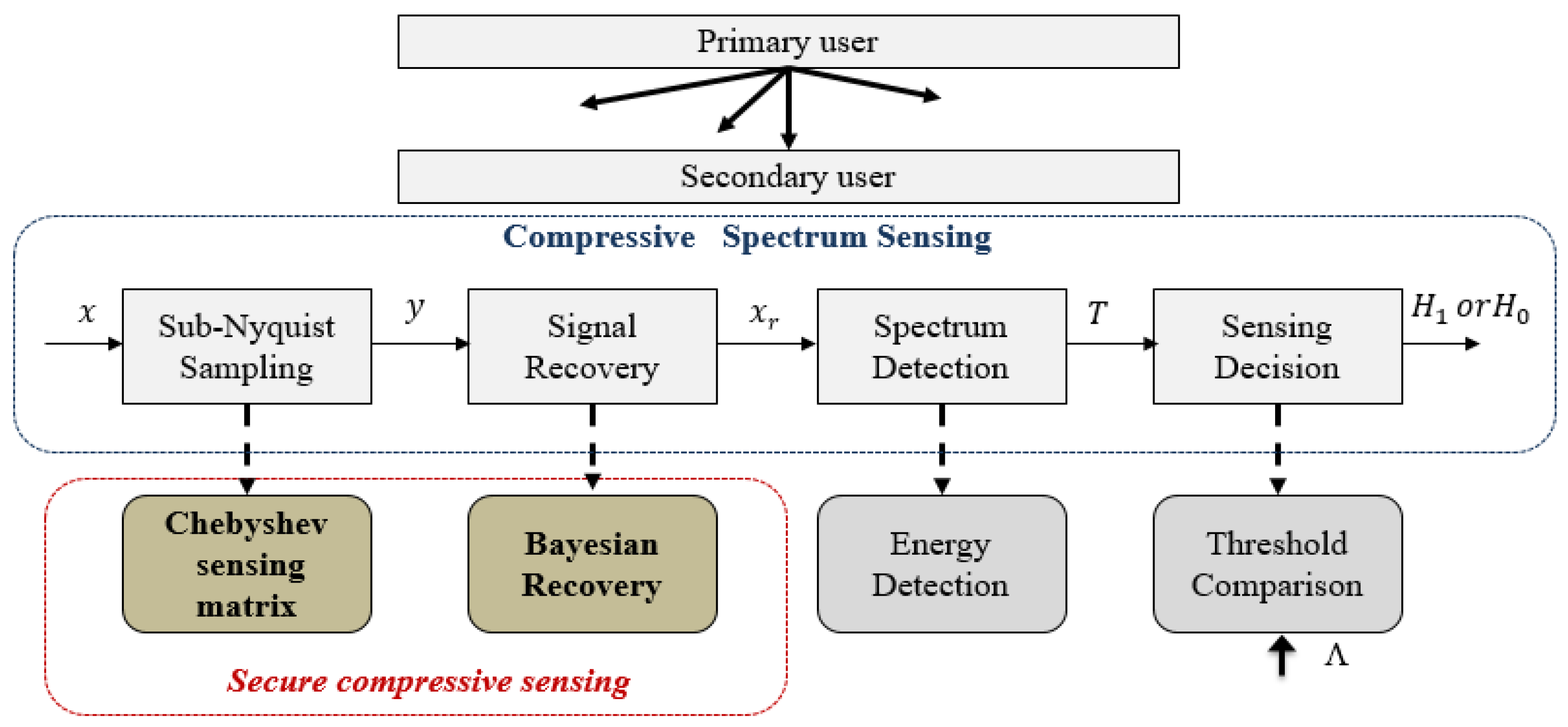
Figure 4 represents the main blocs of the proposed chaotic compressive spectrum sensing approach. It aims at adapting the sparsity and recovering the received signal, x, from a few non-adaptive measurements, y, with high probability. Then, an adapted threshold, Λ, is selected according to the energy-based detection technique. The predefined threshold is compared next with the test statistic, TED, to make the final sensing decision by choosing between the binary hypotheses, H1 (occupied) and H0 (vacant). To simply the system and verify the efficiency of the proposed solution, we focus on a direct communication between a single SU and PU.
3.1. Sub-Nyquist Sampling Based on Chebyshev Sensing Matrix
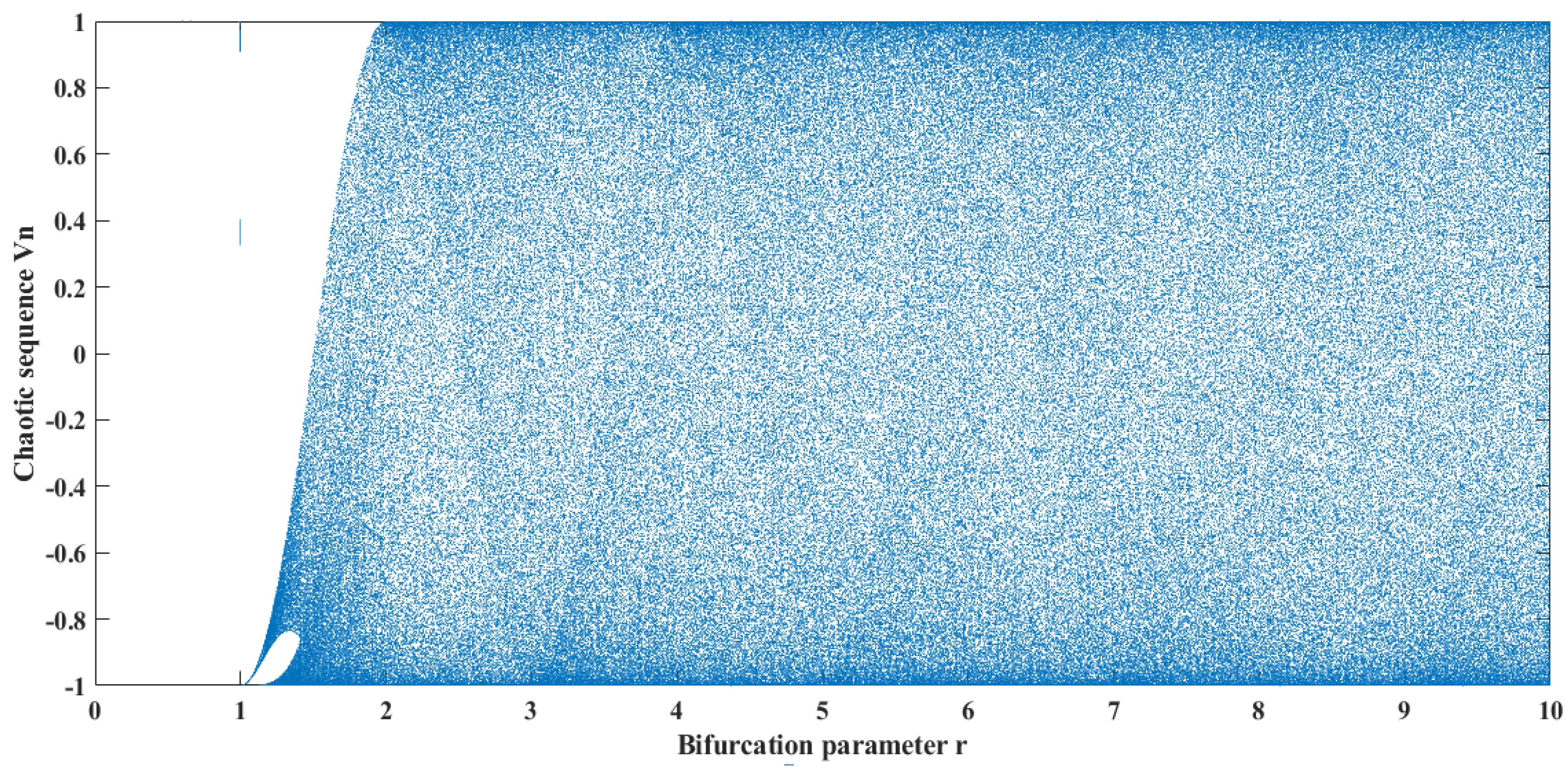
The sub-Nyquist sampling process is performed with the chaotic sensing matrix [37] based on Chebyshev map, to reduce the number of measurements taken from the original signal and to provide an inherent security to the system. The Chebyshev map [25,54] is a discrete chaotic system with an initial condition, V0, and a bifurcation parameter, r, and can be defined by the following recurrence sequence
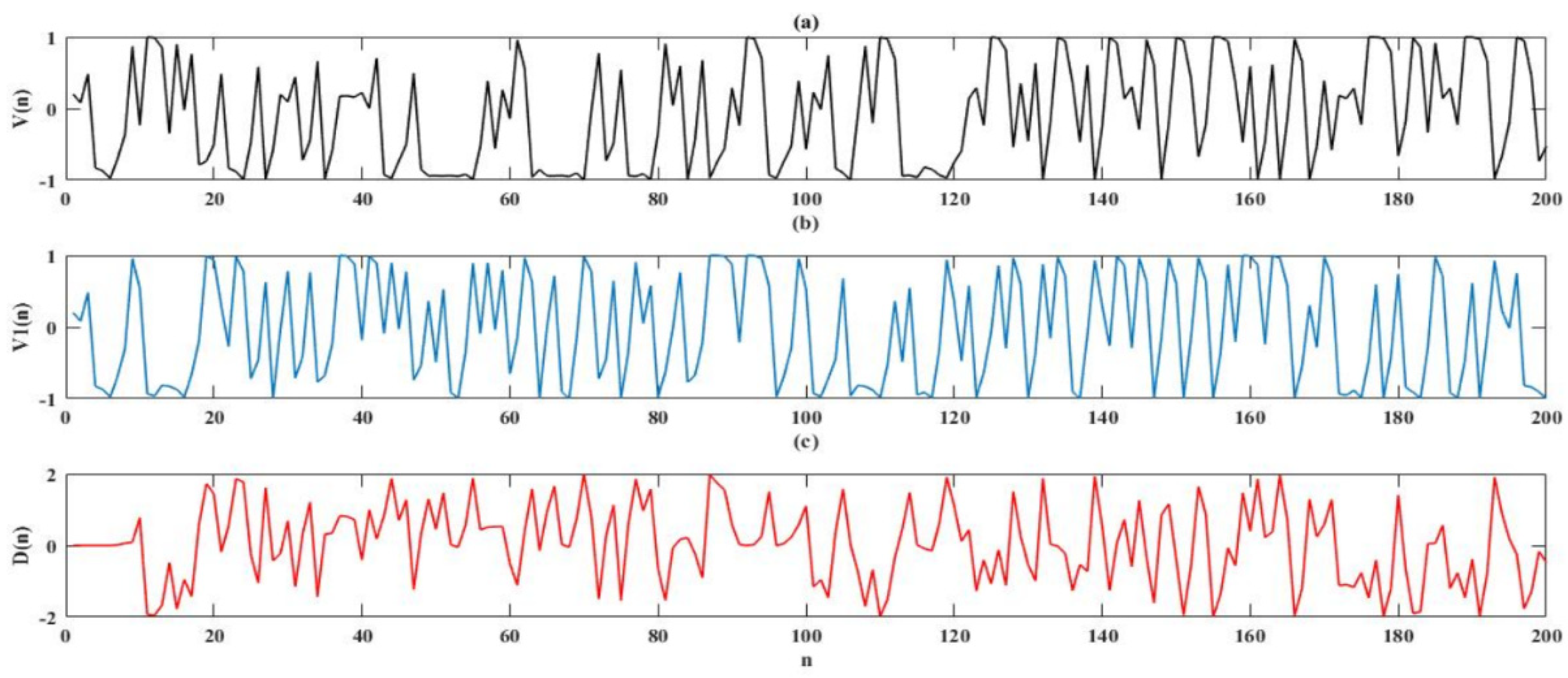
where Vn is the nth term in the recurrence sequence with Vn ∈ [−1, 1] for n = 0, 1,2, … and r ∈ [2,∞). The bifurcation diagram of the Chebyshev map presented in Figure 5 illustrates the chaotic performance for different values of r. As we can see, it is recommended to use values of r greater than 2 where the chaotic behavior is significant. However, the sensitivity to the initial value and the bifurcation parameter is the particularity that makes chaotic systems more relevant. It means that any small change in these parameters generates different sequences. For example, if we fix r = 3.5 in the recurrence sequence (11), and we change V0 with a very small value, i.e., the first sequence uses V0 = 0.2, and the second uses V0 = 0.200001, then we get a significant difference, denoted as D, between the two generated sequences, as shown in Figure 6. This sensitivity makes the Chebyshev sensing matrix a suitable choice for a secure system.
Vn+1 = cos (r cos−1 (Vn))
To design the Chebyshev sensing matrix C ∈ RMxN, we use the sequence described by Equation (11) as V (h, d, V0) = {Vn, Vn+d,…, Vn+hd} with h = 0, 1, 2 …, a sampling distance d and initial condition V0. Then, to verify the randomness of the sensing matrix, the first 1000 trials of the sequence are skipped [37], and we denote the regularization of V (h, d, V0) as follows:
where Ch ∈ C(h,d,c0) is the new sequence that we use to construct our sensing matrix, column by column, such that we get the following:
where is for normalization.
Ch = V1000+hd
The sensitivity to the initial conditions present the key of security of each chaotic matrix that makes this type of matrices a suitable solution to enhance the security in case of cooperative CRNs; only by sharing the accurate initial parameters of the chaotic map can any user in the network perfectly reconstruct the received signal.
3.2. Bayesian Recovery via Laplace Prior
To solve the problem defined by Equation (5), we apply the Bayesian recovery algorithm based on Laplace prior technique [55], to handle uncertainty in measurements. The Bayesian algorithm is a statistical technique that defines all unknown variables through probability distributions. In the proposed model, compressive measurements (y), original signal (x), chaotic sensing matrix (C), and noise (e) are the main parameters in the system. The objective is to provide a full posterior distribution for the values of x based on prior belief, including the sparsity assumption of x and the relationship between the noisy measurements, y, and the received signal, x. To realize this, the Bayesian model requires the definition of a joint distribution P (x, α, β, and y) of all unknown parameters by introducing new variables, α and β, called hyper parameters. To simplify the analysis of the joint distribution, the following factorization is used:
where P (x | α) is a prior distribution which defines our knowledge on the nature of x and P(y | x, β) is the conditional distribution with β = 1/∂2 is the inverse noise variance.
P (x, α, β, y) = P (y | x, β) P (x | α) P (β) P (α)
According to the central limit theorem, when the number of measurements is small compared to the length of the received signal (N ≫ M), the measurements vector y can be approximated as Gaussian distribution with zero mean and a variance β−1 [56]. Hence, the conditional distribution of y, given the sparse signal, x, can be expressed as follows:
P (y | x, β) ~ N (y | Cx, β−1)
To simplify the analysis, the Gamma distribution [55] is used to define the hyper parameter β as follows:
where cβ and dβ are the scale and the shape parameter, respectively, assigned to β. They are called hyper priors.
P (β | cβ, dβ) ~ Γ (β | cβ, dβ)
To exploit the sparsity of the received signal x, a Laplacian density function is used to describe the prior distribution P (x | α) as follows:
P (x | α) = (α/2)N exp (−α‖x‖1)
Next, the Bayesian inference based on an evidence procedure is used, which can be defined by the following decomposition:
where P (x | y, α, β, λ) ∝ P (x, y, α, β, λ), and it can be defined as a multivariate Gaussian distribution [14,55,57] with a mean µ and covariance ∑ given as follows:
P (x, α, λ, β | y) = P (x | y, α, β, λ) P (α, β, λ | y )
µ = β ∑ CTy, ∑ = [βCTC + A]−1 with A = diag (1/αi)
To estimate the hyper parameters used in this procedure, we consider firstly the following factorization:
P (α, β, λ | y ) = [P (y, α, β, λ )/P(y)] ∝ P (y, α, β, λ )
Secondly, we maximize the joint distribution P (y, α, β, λ) or its logarithm L [14,55] given by the following equations:
where J = β−1 I + CA−1CT and I denotes the identity matrix.
Finally, we determinate the derivatives of the logarithm presented by (21) to define the two hyper parameters, β and λ, as follows:
Subsequently we can solve the l1-minimisation problem given by (5).
3.3. Spectrum Detection and Sensing Decision
The spectrum sensing process can be defined as follows:
where N is the number of samples, xr(n) is the SU recovered signal, s(n) is the primary signal, and w(n) is the additive white Gaussian noise (AWGN) with zero mean and variance δw. H0 and H1 denote respectively the absence and the presence of the PU signal.
xr(n) = w(n) H0: PU is absent
xr(n) = s(n) + w(n) H1: PU is present
xr(n) = s(n) + w(n) H1: PU is present
To analyse the SU recovered signal xr(n), the energy-based sensing detection is used. It is performed by comparing between a detector output, TED, and a detection threshold, Λ, to make the final decision about the primary signal occupancy. In our model, the detector output is the input sparse signal energy given by the following:
where N is the number of samples and xr(n) is the SU recovered signal. Therefore, the sensing decision can be formulated as follows:
where Λ is the sensing threshold. In an energy-detection model with a large samples number, the detector output, TED, can be approximated as a Gaussian distribution, according to the central limit theorem [56,58], and given by the following:
where N is the number of samples, and δw and δs are the variance of the noise and the PU signal, respectively. Probability of detection, Pd, and probability of false alarm, Pfa, can be expressed by using the Q-function [58], as follows:
if TED ≥ Λ, H1: PU is present
if TED < Λ, H0: PU is absent
if TED < Λ, H0: PU is absent
From Equation (27), the sensing threshold Λ can be derived as follows:
The sensing threshold is a critical parameter in energy detection. Thus, in our model we adjust the threshold based on the signal sparsity to improve the system performance and to maximize its efficiency. The proposed threshold can be formulated as follows:
To summarize the main steps of our methodology, the pseudocode for the proposed solution can be formulated as follows in Algorithm 1.
| Algorithm 1 Chaotic compressive spectrum sensing |
| Input: Signal length N Number of compressive measurements M Sparsity level K Noise variance δw Signal-to-noise ratio SNR Energy detection threshold Λ |
| Output: Sensing decision H0/H1 |
| Step 1: Define the received signal x -Generate the sparse signal PU: s -Add the channel noise: x = + sδw Step 2: Construct the Chebyshev sensing matrix C -Initial value: V0 -Bifurcation parameter: r -Sampling distance: d -The Chebyshev sequence: Vn+1 = cos (r cos−1 (Vn)) -The regularization of V (h, d, V0): Ch = V1000+hd -Construction of the matrix C: C1 (Vn, M, N) -Normalization of the matrix C: C = C1 Step 3: Generate the noisy compressive measurements: y = Cx + e Step 4: Solve by Bayesian recovery algorithm: xr = argmin Step 5: Perform spectrum detection -Calculate the energy of xr: TED = xr(n)2 -Make the final decision: if TED ≥ Λ, H1: PU is present if TED < Λ, H0: PU is absent |
4. Simulation Results
To investigate the efficiency of the proposed chaotic system, three aspects are discussed: (i) the system performance of signal recovery process, in order to evaluate the strength of the Bayesian model, compared to the two other techniques, convex and greedy algorithms; (ii) the common performance of the proposed system in terms of quality of the sampling matrix and total number of detection, compared with other chaotic sensing matrices: (iii) the sensitivity of the system to the initial conditions of the proposed sampling matrix, to prove its ability to handle security issues when an external user tries to join the network.
For numerical simulations, we generate a discrete sparse signal x of length N = 500 samples and randomly place K = 50 spikes (10% of N). For sampling process, the same chaotic Chebyshev matrix is used in the different comparisons of this paper and generated via Equation (11) with V0 = 0.3, which presents the initial value; r = 3.5 is the bifurcation parameter, and d = 15 denotes sampling distance. To solve the recovery problem, we apply the Bayesian algorithm based on the Laplace prior technique, to speed up the recovery time and deal with uncertainty in measurements. The system performance using this technique is compared to two other recovery techniques, namely BP [59] and OMP [27] algorithms. These algorithms were used because they provide the best performance in two key categories of recovery processes: greedy and convex.
To evaluate the sampling performance of the proposed system, the Chebyshev sensing matrix is tested and compared to random matrix and two other chaotic matrices based on two different maps, the logistic map and the quadratic map, which are defined, respectively, as follows:
where Zn and Gn denote the nth term in the chaotic sequence, with Z0 = G0 = 0.5 as the initial values and r1 = 3.9 and r2 = 1.2 as the bifurcation parameters.
Zn+1 = r1 Zn (1 − Zn)
Gn+1 = r2 − G2n
The following performance metrics are used: mutual coherence [49], recovery error [60], spikes error rate (SER), sampling time, recovery time, processing time, probability of detection (Pd), and probability of false detection (Pfd). The coherence is one of the main requirement of compressive sensing to ensure a robust recovery of the signal. It evaluates the sensing matrix quality and its efficacy by using Equation (3). The recovery error is defined as the distance between the estimated signal and the original signal, x. It is formulated as follows:
The spikes error rate SER evaluates the error rate of the recovered signal spikes. It calculates the sum of the false and missed spikes divided by the signal’s length. It is given by the following equation:
where Nfs and Nms denote the number of false and missed recovered spikes, respectively. The sampling time metric evaluates the speed of a sensing matrix. It refers to the time required for acquisition process using a particular sensing matrix. Recovery time is the elapsed time during the reconstruction process. Processing time is the time needed to perform the whole algorithms, including acquisition process, recovery process, and sensing decision process. The probabilities of detection and false detection are computed by the following:
where Nd is the total number of detections, Nfd is the total number of miss detections, and Nt is the number of total trials.
The performance results of the first aspect are presented in Figure 7 and Figure 8, which illustrate a comparison results between three recovery algorithms, i.e., Bayesian, BP, and OMP algorithms, with the Chebyshev sensing matrix.
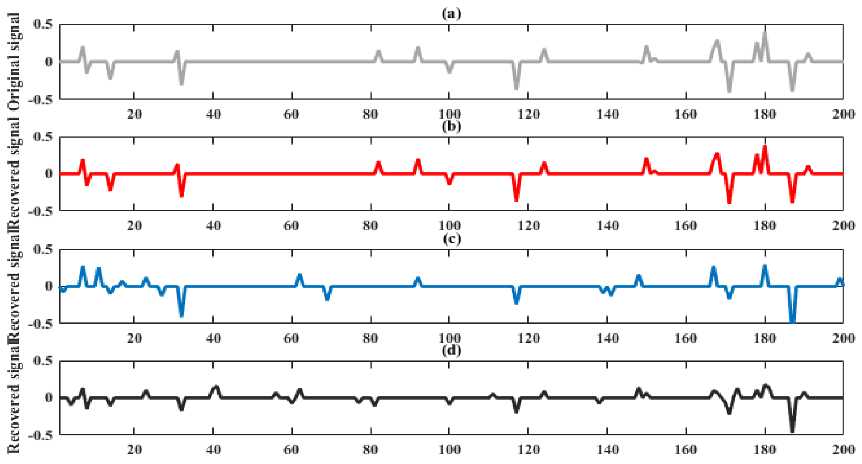
Figure 7a shows an example of a sparse signal with N = 200 samples and K = 15 spikes for a signal-to-noise ratio (SNR) of −10 dB. Figure 7b–d presents the output signal using the Chebyshev matrix according to (11) with the Bayesian recovery, BP and OMP algorithms, respectively. As we can see in Figure 7b, the Bayesian recovery is more efficient in combination with the Chebyshev sensing matrix and gives a more similar output signal to the input one. However, the estimated signal using the BP and OMP algorithms reveals some variations, as shown in Figure 7c,d. As a result, our proposed combination is efficient and reliable.
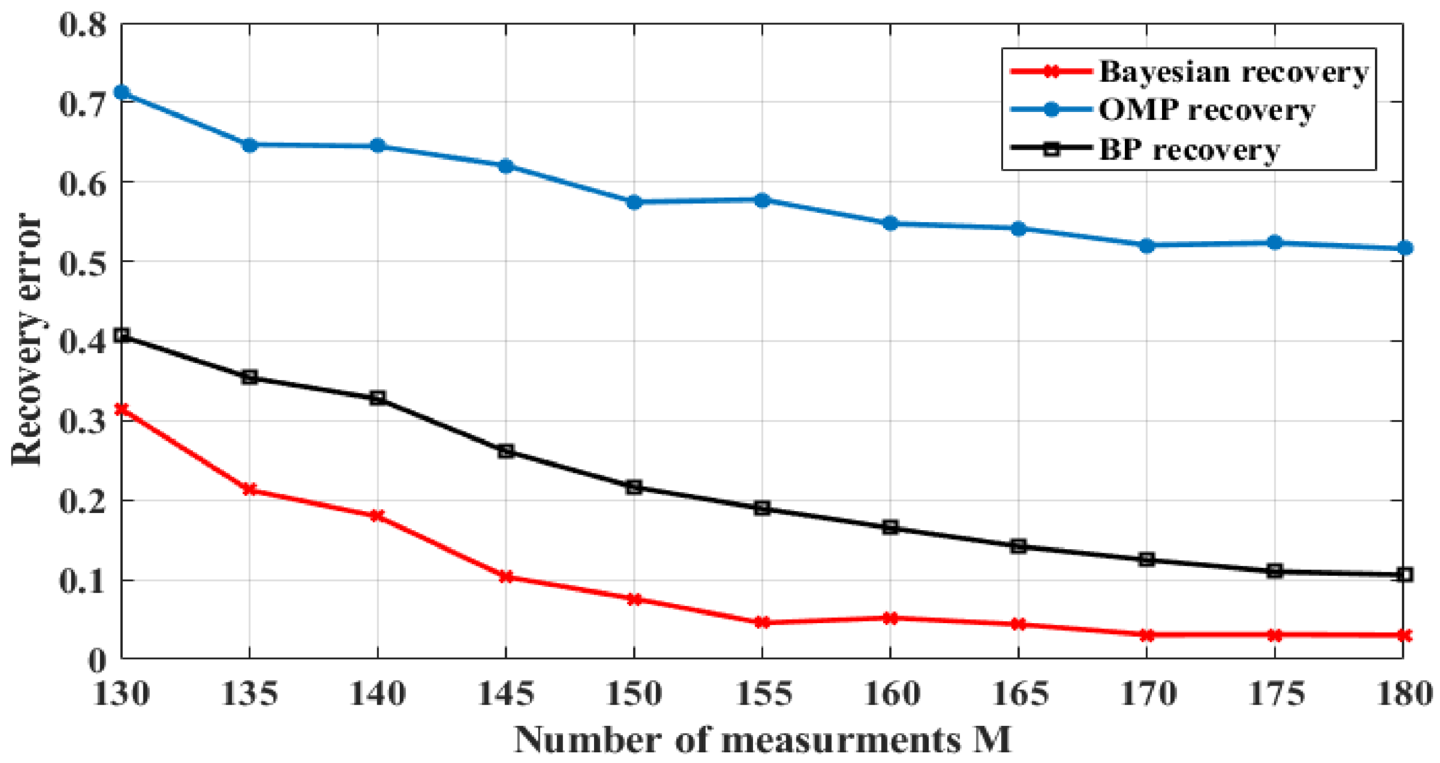
Figure 8 shows the comparison results based on the recovery error metric for multiple values of the compressive measurements, M, with SNR = −10 dB. As we can see, the three recovery algorithms minimize the recovery error with the growth of number measurements, M. However, these results show that OMP has a high recovery error compared to other recovery techniques, since the Bayesian model gives the best error rate with the lowest number of measurements.
As presented in Table 1, this work shows that using the Chebyshev-based Compressive sensing with OMP is fast but uncertain and presents a high recovery error level; the BP algorithm is slower and shows a good recovery error level, but it is uncertain and more complex; and the Bayesian recovery is the fastest, is less complex, deals with uncertainty, and provides low recovery error. This means that our combination is the most balanced and efficient one.
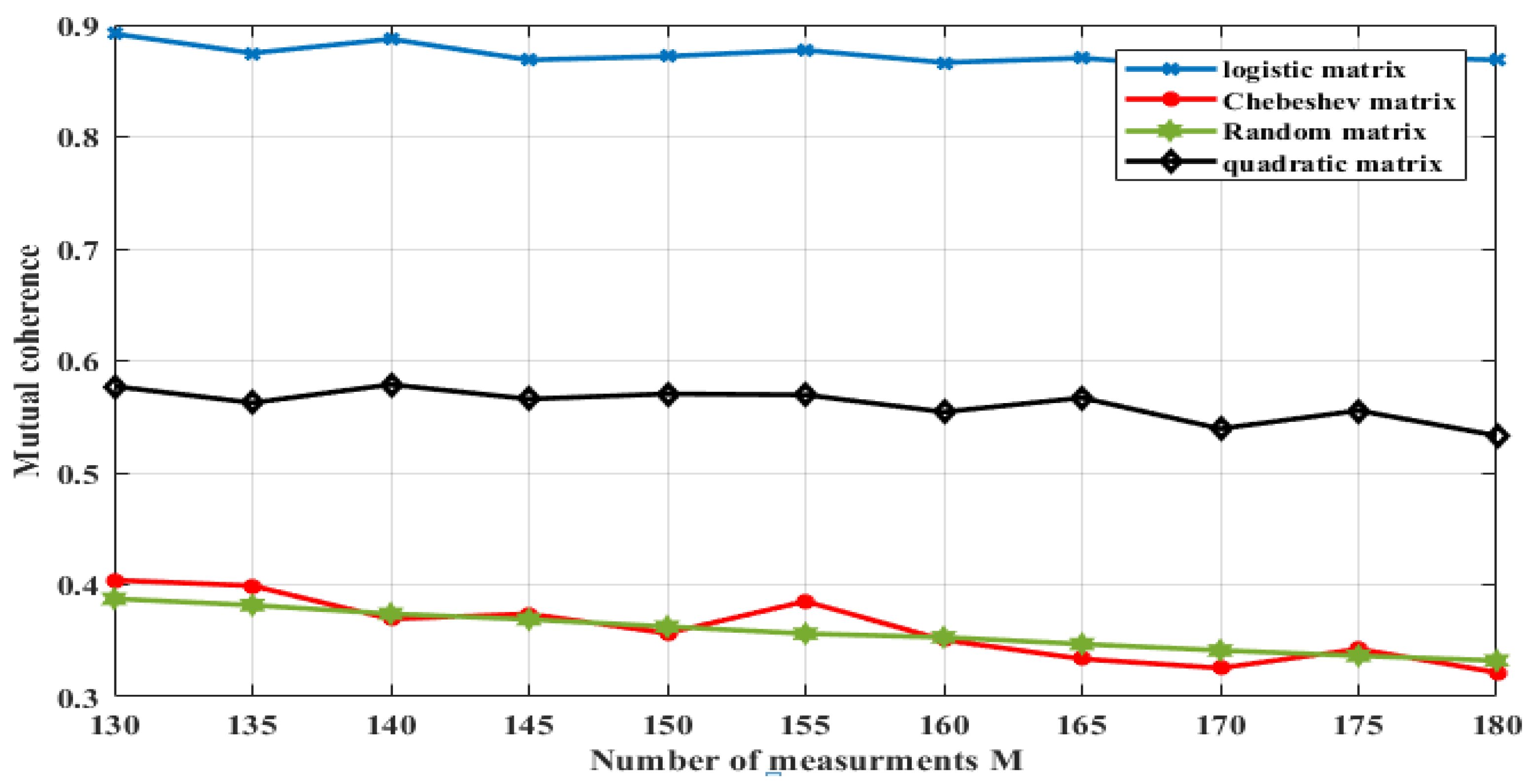
For the second aspect, we start our analysis by the study of the mutual coherence for different sensing matrices as shown in Figure 9, where we plotted the mutual coherence against the number of measurements M. The matrices considered for this test include thw random matrix and three different chaotic matrices based on different sequences: the logistic sequence, according to Reference [30]; the quadratic sequence, according to Reference [31]; and the Chebyshev matrix, according to Reference [11]. The figure shows that Chebyshev matrix, in some points, is similar to the random matrix, and both present a low coherence when compared to the other matrices. Thus, the significant differences existing between chaotic matrices prove the efficiency of the Chebyshev matrix that can perform well with less measurements. Furthermore, the Chebyshev sensing matrix is deterministic; therefore, it is more practical to construct and transmit than random matrices. It means that the proposed sensing matrix can replace the commonly used random one.
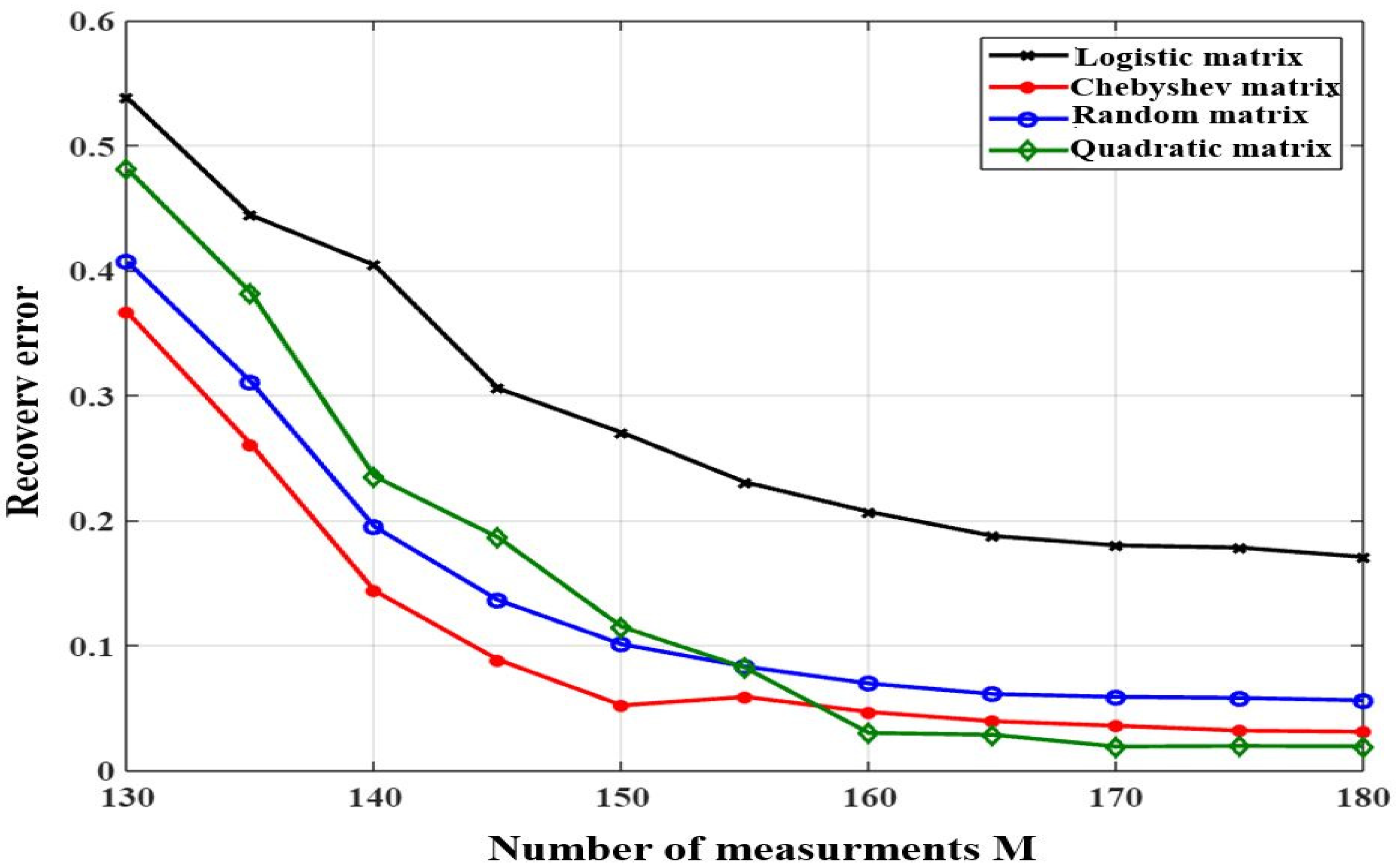
Figure 10 shows the comparison results based on the recovery error metric for multiple values of the compressive measurements M. As we can see, all sensing matrices considered in this simulation minimize the recovery error with the growth of number measurements, M. However, the difference in the performance results between the sensing matrices is substantial and significant, especially from M = 130 to M = 155. It is worth noting that the Chebyshev matrix performs better than the other sensing matrices, since it achieves an acceptable error rate with a minimum amount of measurements, M = 130 = 26% of N. Hence, the Chebyshev matrix is a suitable choice to improve the performance of the proposed system in both acquisition and recovery process, in terms of sampling time and computational complexity, by acquiring the received signal with the lowest number of measurements and an acceptable recovery error.
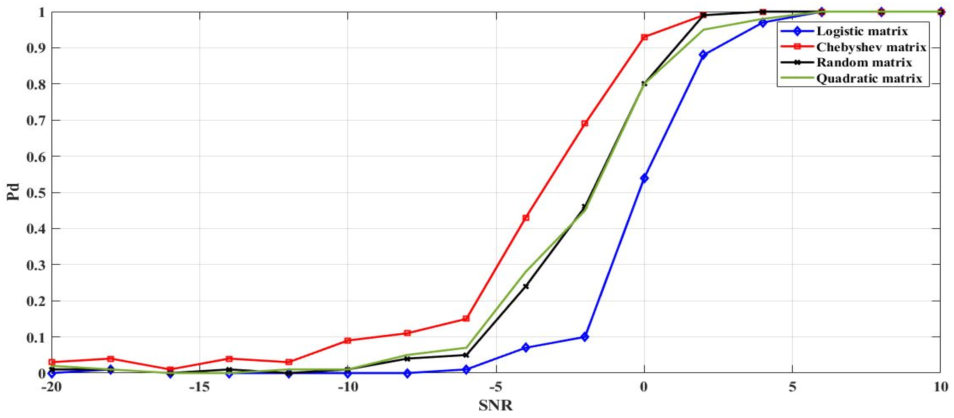
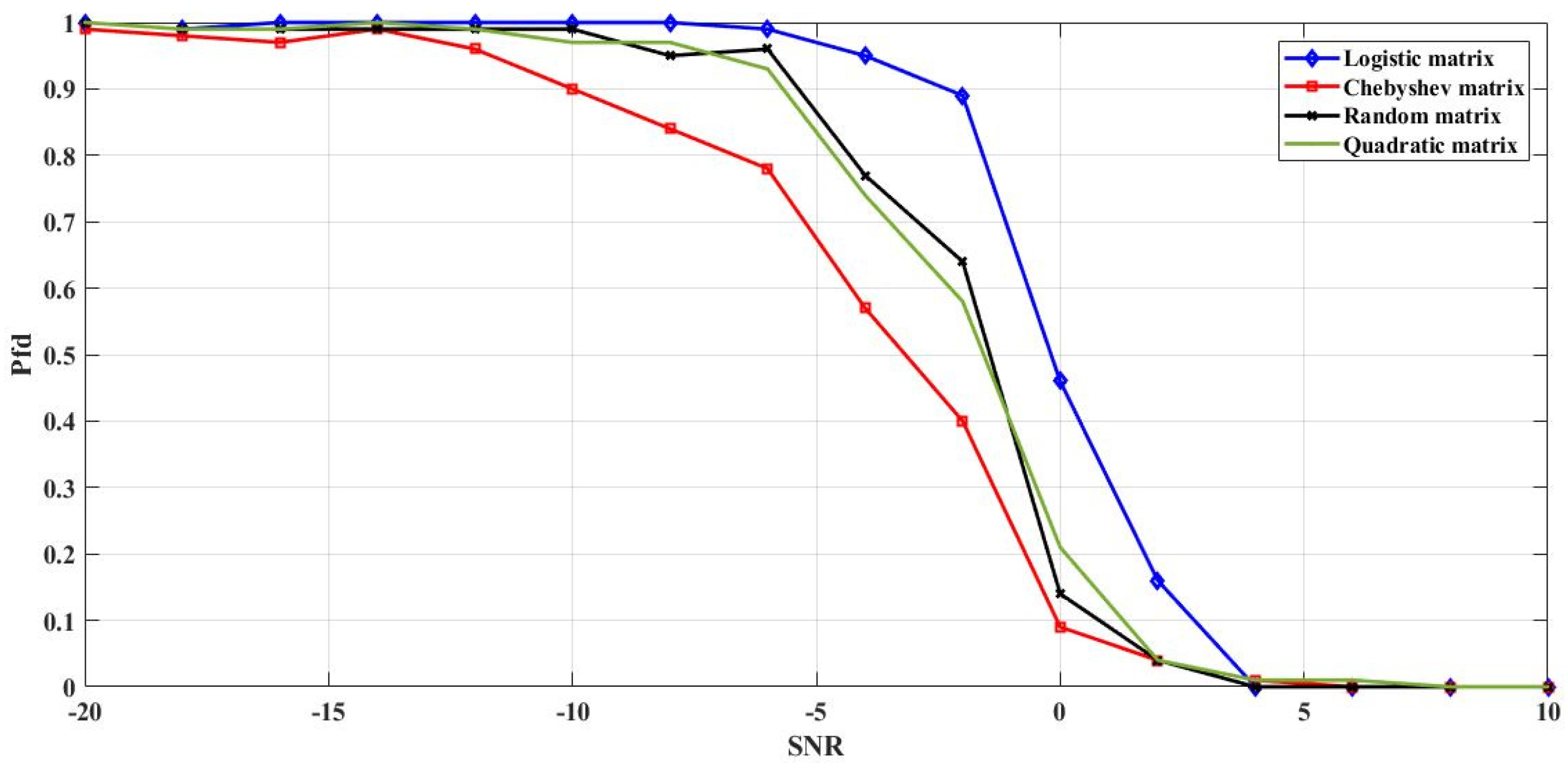
As for spectrum sensing process, to evaluate the efficiency of the proposed solution, we performed different comparisons between the probabilities of detection and false detection versus SNR. Examples of results are presented in Figure 11, Figure 12, Figure 13 and Figure 14. The SNR values’ range is from −20 dB to +10 dB. Figure 11 presents the probability of detection as a function of SNR for Logistic, Chebyshev, quadratic, and random sensing matrices with a probability for false alarm (Pfa) of 0.01. This figure also illustrates that the probability of detection increases proportionally with SNR for all sensing matrices, to reach 100% for SNR = 5 dB. It is also noted that the probability of detection, based on the Chebyshev sensing matrix, increases faster than the other matrices for lower SNR values. However, Figure 12 shows the opposite of the above result, where the probability of false detection of the proposed Chebyshev sensing matrix decreases faster than the logistic, quadratic, and the random matrices, to reach 0% for SNR = 4 dB.
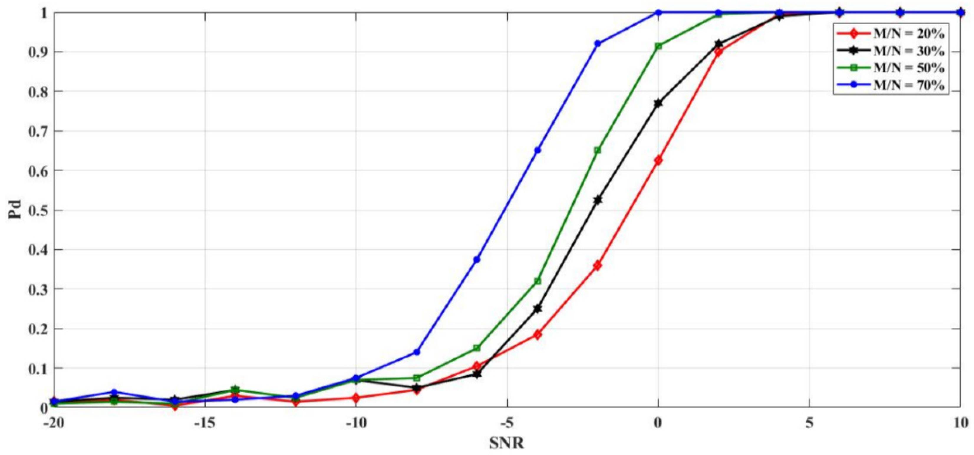
Figure 13 presents the probability of detection against SNR for compressive spectrum sensing based on Chebyshev matrix for four different values of the compression ratio, M/N = 20%, 30%, 50%, and 70%. One can see, for a compression ratio M/N = 70%, the probability of detection reaches 100% for SNR = 0 dB for M/N = 50%, the probability of detection meets 100% for SNR = 2 dB, and for M/N = 30% = 20% the probability of detection achieves 100% for SNR = 5 dB. This means that we can reduce the compressive measurements, M, until 20% of N and still get a substantial performance.
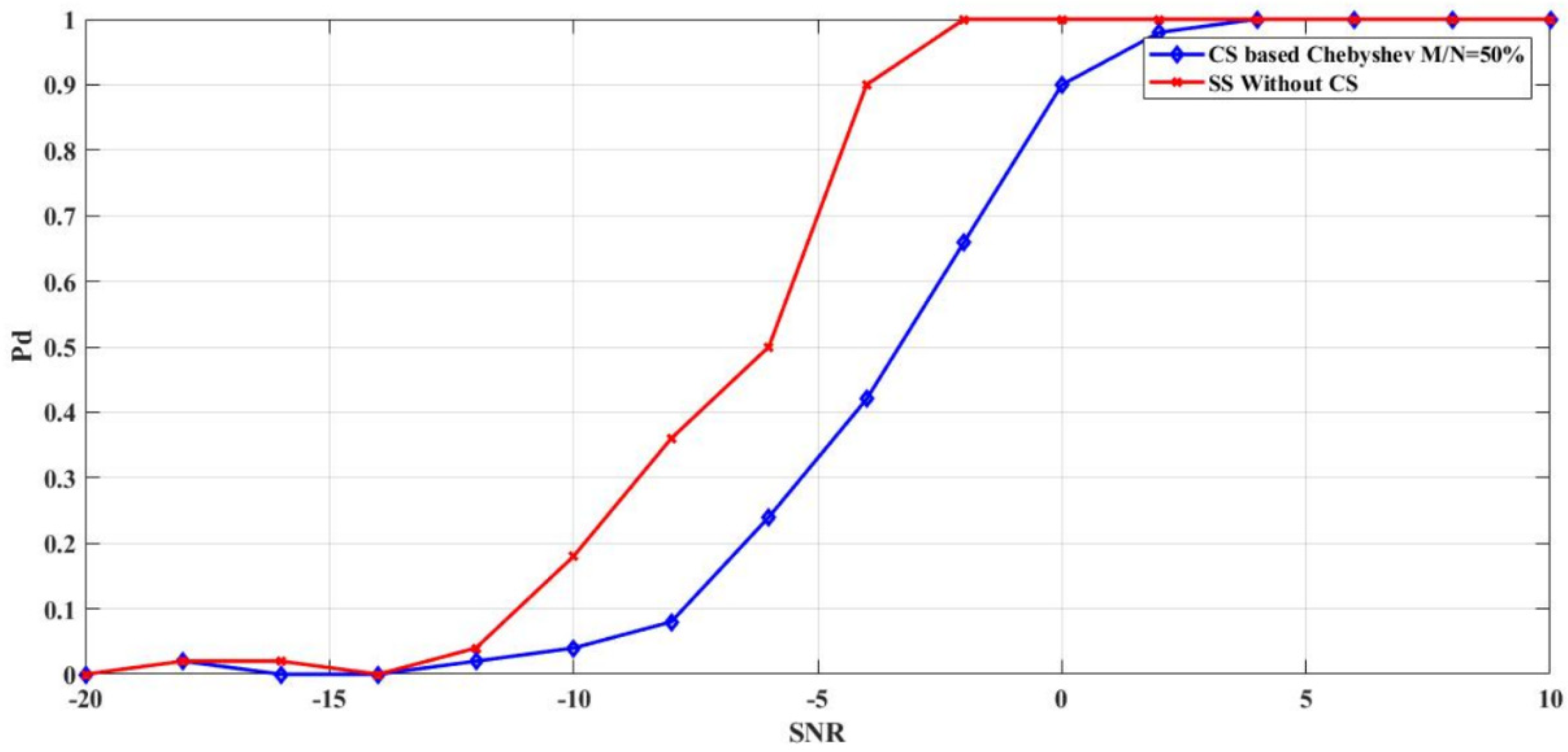
Figure 14 shows the probability of detection as a function of the SNR for two techniques: chaotic CSS and normal sensing without compressive sensing. As shown in the figure, for probability of false alarm Pfa = 0.01 the probability of detection growths as the SNR increase for both techniques, the proposed model and the normal sensing. It can also be noted that the probability of detection without compressive sensing reaches 100% for SNR= −2 dB, while the probability of detection of our proposed model with a compression ratio M/N = 50% achieves 100 % for SNR = 2 dB. It means that, with a smaller number of measurements, we can still maintain appropriate detection performance close to the normal sensing.
Sampling time is another metric used to evaluate the performance of the system, using different sensing matrices, in terms of the speed of signal acquisition. Examples of the comparison results are presented in Table 2. As expected, the simulation results show that the Chebyshev sensing matrix requires a lower value of sensing time.
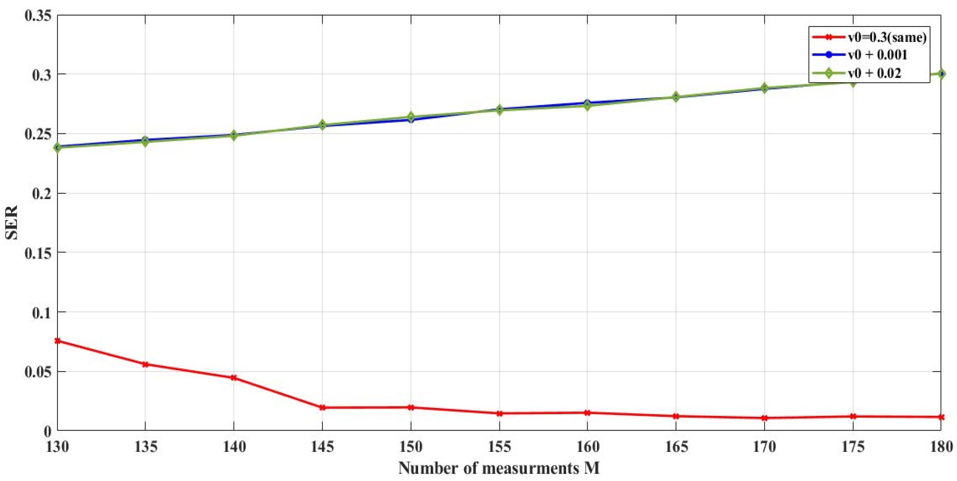
Next, to verify the sensitivity of the system to the initial parameters of the chaotic Chebyshev matrix, we used two different matrices: the first one for the acquisition process and the second for the recovery process. The sensing matrix generated in reconstruction process used different initial parameters (different bifurcation parameters, r, and initial values, V0).
Figure 15 shows an example of the comparison results in the case of using a Chebyshev map according to (11), with the same initial value (V0 = 0.3) in both the acquisition and reconstruction step and three other matrices with different initial values (V0+0.001 and V0+0.02) in the reconstruction step. As we can see, any minor variations in the initial value produce a different sequence for the sensing matrix, which generates a different recovered signal with a high error rate. This means that it is very difficult for an outside user to use the network without having prior information about the initial conditions used to produce the sensing matrix.
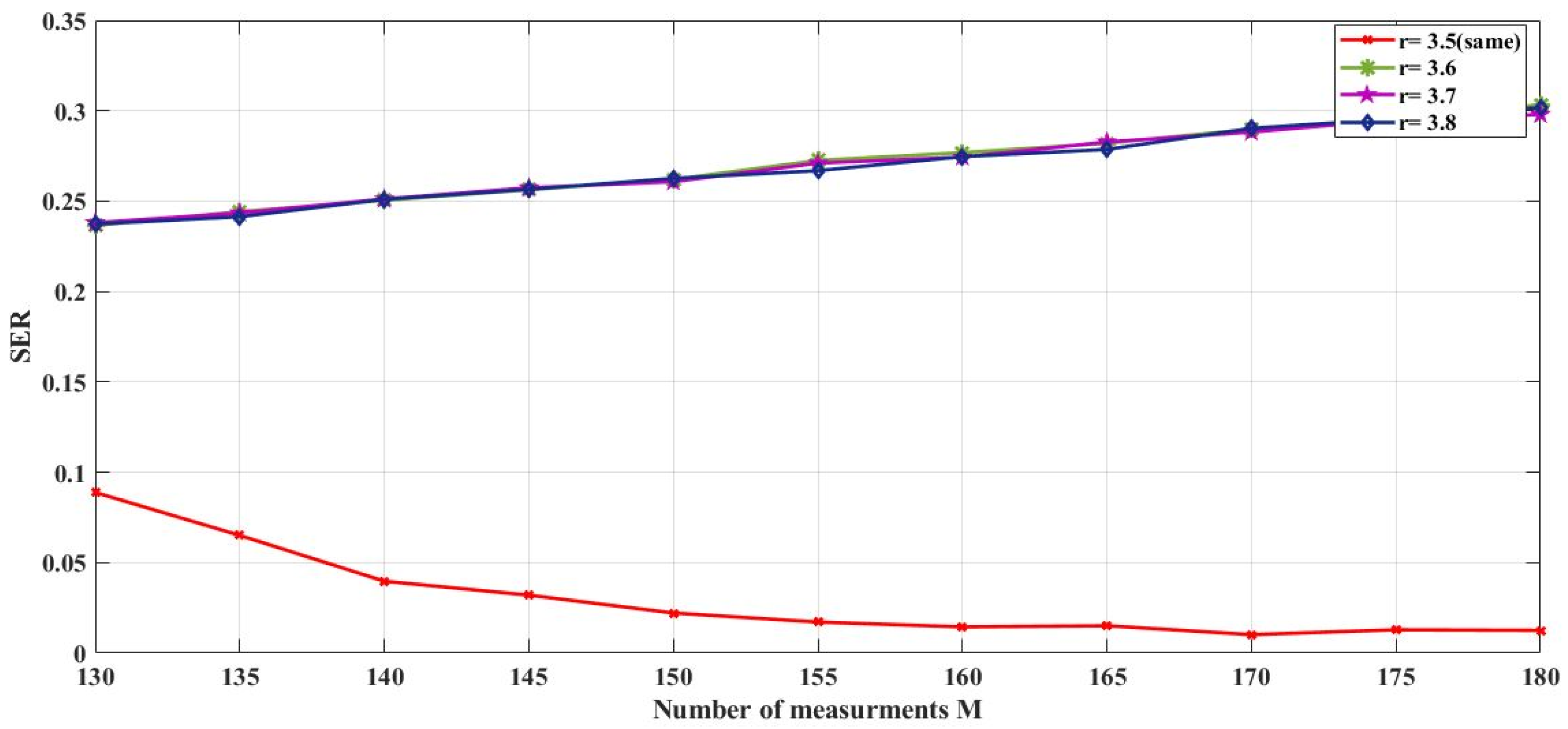
In Figure 16, the same test is executed, but this time the bifurcation parameter, r, is modified. The transmitter uses r = 3.5 to generate the Chebyshev chaotic matrix, and we evaluate the system performance of four receivers, using r = 3.5, 3.6, 3.7, and 3.8. As expected, only users that use the same bifurcation parameter at the reconstruction process are able to recover the signal with a low error rate. Thus, the proposed system is very sensitive to both the initial value and bifurcation parameter.
Table 3 summarizes examples of the different performance comparisons performed in this work. Column (1) shows the results according to the normal sensing technique. Columns (2)–(5) present examples of simulation performance resulting from the compressive spectrum sensing based on different sensing matrices: Chebyshev matrix, logistic matrix, quadratic matrix, and random matrix. As one can see, for the probability of false alarm, Pfa = 0.01 and SNR = 0 dB, the normal sensing reaches a probability of detection of 100%. However, the compressive spectrum sensing based on different sensing matrices meets 92%, 80%, 55%, and 80% for SNR = 0 dB for the sensing matrices Chebyshev, quadratic, logistic, and random, respectively. For the recovery error, the compressive spectrum sensing based on different sensing matrices has a recovery error values of 0.023, 0.02, 0.18, and 0.05, for the sensing matrices, Chebyshev, quadratic, logistic, and random, respectively. For the coherence metric, Chebyshev and random matrices both present a low coherence value of 0.32 and 0.33, respectively, compared to the other sensing matrices, quadratic and logistic. It means that the Chebyshev matrix can perform well with a lower number of measurements. For the processing time of the normal sensing is 33 ms, while the time for the compressive spectrum sensing based on different sensing matrices is 24, 26.3, 25.4, and 28 ms, for the sensing matrices Chebyshev, quadratic, logistic, and random, respectively. To summarize, we can conclude that the proposed combination between the Bayesian recovery and Chebyshev sensing matrix is reliable, robust, and faster, since with only 50% of compressive measurements, the probability of detection decreases by 8%, but the processing time is reduced by approximately 27%.
5. Conclusions
In this paper, a novel chaotic CSS solution is proposed for cooperative CRNs. This solution aims at improving the acquisition and recovery processes by taking into consideration three aspects, namely the security issues, time, and the uncertainty in measurements. Our proposed model provides a robust combination, using a chaotic sensing matrix based on Chebyshev map and Bayesian recovery algorithm via Laplace prior. The Chebyshev sensing matrix has the advantages of the deterministic matrices; thus, it can be easily performed and shared between the different nodes of the cooperative network, unlike random matrices, which need extra memory capacity and more time to be stored and shared over the network. However, the most interesting benefit of this type of matrix is that it provides an integral security of the system, since a slight change in the initial parameters generates a different sensing matrix. This property makes it difficult to unauthorized users to join the cooperative network without having adequate information about the parameters used to generate the sensing matrix. For the recovery process, a strong Bayesian inference based on Laplace prior technique is used to handle uncertainty in measurements. To evaluate the proposed technique, we opt for several performance metrics, including coherence, recovery error, spikes error rate, sampling time, recovery time, processing time, probability of detection, and probability of false detection. Through analyzing the simulation results, we can conclude that the Bayesian algorithm with the Chebyshev sensing matrix is more efficient than the Bayesian algorithm with the logistic, quadratic, and random matrices. In addition, the proposed combination provides superior performances, but with less compressive measurements, which can be reduced to 20% of the signal’s length. In further work, we will extend the scenario to multiple SUs, and we also plan to focus on improving the spectrum sensing process by using other techniques to continue reducing the number of measurements.
Author Contributions
Conceptualization, S.B.; methodology, S.B., M.R. and F.S.; software, S.B.; validation, S.B., M.R. and F.S.; formal analysis, S.B., M.R. and F.S.; investigation, S.B.; resources, S.B., M.R. and F.S.; data curation, S.B., M.R. and F.S.; writing—original draft preparation, S.B.; writing—review and editing, S.B., M.R. and F.S.; visualization, S.B., M.R. and F.S.; supervision, M.R., F.S. and A.H.; project administration, A.H. All authors have read and agreed to the published version of the manuscript.
Funding
This research received no external funding.
Institutional Review Board Statement
Not applicable.
Informed Consent Statement
Not applicable.
Data Availability Statement
Not applicable.
Conflicts of Interest
The authors declare no conflict of interest.
References
- Ridouani, M.; Hayar, A.; Haqiq, A. Relaxed constraint at cognitive relay network under both the outage probability of the primary system and the interference constrain. In Proceedings of the IEEE European Conference on Networks and Communications, London, UK, 8–12 June 2015; pp. 1–6. [Google Scholar]
- Elrhareg, H.; Ridouani, M.; Hayar, A. Routing Protocols on Cognitive Radio Networks: Survey. In Proceedings of the IEEE International Smart Cities Conference, Casablanca, Morocco, 14–17 October 2019; pp. 296–302. [Google Scholar] [CrossRef]
- Salahdine, F.; Kaabouch, N.; El Ghazi, H. Techniques for dealing with uncertainty in cognitive radio networks. In Proceedings of the IEEE 7th Annual Computing and Communication Workshop and Conference, Las Vegas, NV, USA, 9–11 January 2017; pp. 1–6. [Google Scholar] [CrossRef]
- Ejaz, W.; Hattab, G.; Cherif, N.; Ibnkahla, M.; Abdelkefi, F.; Siala, M. Cooperative Spectrum Sensing with Heterogeneous Devices: Hard Combining Versus Soft Combining. IEEE Syst. J. 2018, 12, 981–992. [Google Scholar] [CrossRef]
- Ben Halima, N.; Boujemaa, H. Cooperative Spectrum Sensing with Distributed/Centralized Relay Selection. Wirel. Pers. Commun. 2020, 115, 611–632. [Google Scholar] [CrossRef]
- Mengbo, Z.; Lunwen, W.; Yanqing, F. Distributed cooperative spectrum sensing based on reinforcement learning in cognitive radio networks. Int. J. Electron. Commun. 2018, 94, 359–366. [Google Scholar]
- Salahdine, F.; Kaabouch, N. Security threats, detection, and countermeasures for physical layer in cognitive radio networks: A survey. Phys. Commun. 2020, 39, 101001. [Google Scholar] [CrossRef]
- Arabia-Obedoza, M.R.; Rodriguez, G.; Johnston, A.; Salahdine, F.; Kaabouch, N. Social Engineering Attacks A Reconnaissance Synthesis Analysis. In Proceedings of the 11th IEEE Annual Ubiquitous Computing, Electronics and Mobile Communication Conference (UEMCON), New York, NY, USA, 28–31 October 2020; pp. 843–848. [Google Scholar] [CrossRef]
- Benazzouza, S.; Ridouani, M.; Salahdine, F.; Hayar, A. A Survey on Compressive Spectrum Sensing for Cognitive Radio Networks. In Proceedings of the IEEE International Smart Cities Conference (ISC2), Casablanca, Morocco, 14–17 October 2019; pp. 535–541. [Google Scholar] [CrossRef] [Green Version]
- Tian, Z.; Giannakis, G.B. Compressed Sensing for Wideband Cognitive Radios. In Proceedings of the IEEE International Conference on Acoustics, Speech and Signal Processing—ICASSP ’07, Honolulu, HI, USA, 15–20 April 2007; Volume 4, p. IV-1357. [Google Scholar] [CrossRef]
- Tian, Z. Compressed Wideband Sensing in Cooperative Cognitive Radio Networks. In Proceedings of the IEEE GLOBECOM 2008–2008 IEEE Global Telecommunications Conference, New Orleans, LA, USA, 30 November–4 December 2008; pp. 1–5. [Google Scholar] [CrossRef] [Green Version]
- Ridouani, M.; Hayar, A.; Haqiq, A. Continuous transmit in cognitive radio systems: Outage performance of selection decode-and-forward relay networks over Nakagami-m fading channels. EURASIP J. Wirel. Commun. Netw. 2015, 2015, 102. [Google Scholar] [CrossRef] [Green Version]
- Ridouani, M.; Hayar, A.; Haqiq, A. Perform sensing and transmission in parallel in cognitive radio systems: Spectrum and energy efficiency. Digit. Signal Process. 2017, 62, 65–80. [Google Scholar] [CrossRef]
- Arjoune, Y.; Kaabouch, N. Wideband Spectrum Sensing: A Bayesian Compressive Sensing Approach. Sensors 2018, 18, 1839. [Google Scholar] [CrossRef] [Green Version]
- Salahdine, F.; El Ghazi, H.; Kaabouch, N.; Fihri, W.F. Matched filter detection with dynamic threshold for cognitive radio networks. In Proceedings of the International Conference on Wireless Networks and Mobile Communications (WINCOM), Marrakech, Morocco, 20–23 October 2015; pp. 1–6. [Google Scholar] [CrossRef]
- Khalfi, B.; Zaid, A.; Hamdaoui, B. When machine learning meets compressive sampling for wideband spectrum sensing. In Proceedings of the 13th International Wireless Communications and Mobile Computing Conference (IWCMC), Valencia, Spain, 26–30 June 2017; pp. 1120–1125. [Google Scholar] [CrossRef]
- El-Khamy, S.E.; El-Mahallawy, M.S.; Youssef, E.-N.S. Improved wideband spectrum sensing techniques using wavelet-based edge detection for cognitive radio. In Proceedings of the International Conference on Computing, Networking and Communications (ICNC), San Diego, CA, USA, 28–31 January 2013; pp. 418–423. [Google Scholar] [CrossRef]
- Hayar, A. Process for Sensing Vacant Bands over the Spectrum Bandwidth and Apparatus for Performing the Same Based on Sub Space and Distributions Analysis. European Patent 08368002.5, 1 February 2008. [Google Scholar]
- Arjoune, Y.; Kaabouch, N.; El ghazi, H.; Tamtaoui, A. A performance comparison of measurement matrices in compressive sensing. Int. J. Commun. Syst. 2018, 31, e3576. [Google Scholar] [CrossRef]
- Thu, L.N.; Shin, Y. Deterministic sensing matrices in compressive sensing: A survey. Sci. World J. 2013. [Google Scholar] [CrossRef] [Green Version]
- Salahdine, F.; Kaabouch, N.; El Ghazi, H. A Bayesian recovery technique with Toeplitz matrix for compressive spectrum sensing in cognitive radio networks. Int. J. Commun. Syst. 2017, 30, e3314. [Google Scholar] [CrossRef]
- Salahdine, F.; Kaabouch, N.; El Ghazi, H. Bayesian compressive sensing with circulant matrix for spectrum sensing in cognitive radio networks. In Proceedings of the IEEE 7th Annual Ubiquitous Computing, Electronics and Mobile Communication Conference (UEMCON), New York, NY, USA, 20–22 October 2016; pp. 1–6. [Google Scholar] [CrossRef] [Green Version]
- Suneel, M. Electronic circuit realization of the logistic map. Sadhana 2006, 31, 69–78. [Google Scholar] [CrossRef] [Green Version]
- Ramadan, N.; Ahmed, H.H.; Elkhamy, S.E.; Abd-El-Samie, F.E. Chaos-based image encryption using an improved quadratic chaotic map. Am. J. Signal Process. 2016, 6, 1–13. [Google Scholar]
- Gan, H.; Li, Z.; Li, J.; Wang, X.; Cheng, Z. Compressive sensing using chaotic sequence based on Chebyshev map. Nonlinear Dyn. 2014, 78, 2429–2438. [Google Scholar] [CrossRef]
- Li, C.; Luo, G.; Qin, K.; Li, C. An image encryption scheme based on chaotic tent map. Nonlinear Dyn. 2017, 87, 127–133. [Google Scholar] [CrossRef]
- Rani, M.; Dhok, S.B.; Deshmukh, R.B. A Systematic Review of Compressive Sensing: Concepts, Implementations and Applications. IEEE Access 2018, 6, 4875–4894. [Google Scholar] [CrossRef]
- Salahdine, F.; Kaabouch, N.; El Ghazi, H. A survey on compressive sensing techniques for cognitive radio networks. Phys. Commun. 2016, 20, 61–73. [Google Scholar] [CrossRef] [Green Version]
- Gao, Y.; Chen, Y.; Ma, Y. Sparse-Bayesian-Learning-Based Wideband Spectrum Sensing with Simplified Modulated Wideband Converter. IEEE Access 2018, 6, 6058–6070. [Google Scholar] [CrossRef]
- Yu, L.; Barbot, J.P.; Zheng, G.; Sun, H. Compressive Sensing with Chaotic Sequence. IEEE Signal Process. Lett. 2010, 17, 731–734. [Google Scholar] [CrossRef] [Green Version]
- Kafedziski, V.; Stojanovski, T. Compressive sampling with chaotic dynamical systems. In Proceedings of the 19thTelecommunications Forum (TELFOR), Belgrade, Serbia, 22–24 November 2011; pp. 695–698. [Google Scholar]
- Gan, H.; Xiao, S.; Zhao, Y. A large class of chaotic sensing matrices for compressed sensing. Signal Process. 2018, 149, 193–203. [Google Scholar] [CrossRef]
- Gan, H.; Xiao, S.; Zhang, Z.; Shan, S.; Gao, Y. Chaotic Compressive Sampling Matrix: Where Sensing Architecture Meets Sinusoidal Iterator. Circuits Syst. Signal Process. 2019, 39, 1581–1602. [Google Scholar] [CrossRef]
- Zeng, L.; Zhang, X.; Chen, L.; Cao, T.; Yang, J. Deterministic Construction of Toeplitzed Structurally Chaotic Matrix for Compressed Sensing. Circuits Syst. Signal Process. 2015, 34, 797–813. [Google Scholar] [CrossRef]
- Yao, S.; Wang, T.; Shen, W.; Shaoming, P.; Chong, Y. Research of incoherence rotated chaotic measurement matrix in compressed sensing. Multimed. Tools Appl. 2015, 76, 17699–17717. [Google Scholar] [CrossRef]
- Gan, H.; Xiao, S.; Zhao, Y.; Xue, X. Construction of efficient and structural chaotic sensing matrix for compressive sensing. Signal Process. Image Commun. 2018, 68, 129–137. [Google Scholar] [CrossRef]
- Kamel, S.H.; Abd-El-Malek, M.B.; El-Khamy, S.E. Compressive spectrum sensing using chaotic matrices for cognitive radio networks. Int. J. Commun. Syst. 2019, 32, e3899. [Google Scholar] [CrossRef]
- Linh-Trung, N.; Minh-Chinh, T.; Tran-Duc, T.; Le, H.V.; Do, M.N. Chaotic Compressed Sensing and Its Application to Magnetic Resonance Imaging. REV J. Electron. Commun. 2014, 3, 84–92. [Google Scholar] [CrossRef]
- Peng, H.; Tian, Y.; Kurths, J.; Li, L.; Yang, Y.; Wang, D. Secure and Energy-Efficient Data Transmission System Based on Chaotic Compressive Sensing in Body-to-Body Networks. IEEE Trans. Biomed. Circuits Syst. 2017, 11, 558–573. [Google Scholar] [CrossRef] [PubMed]
- Xie, D.; Peng, H.; Li, L.; Yang, Y. An efficient privacy-preserving scheme for secure network coding based on compressed sensing. AEU Int. J. Electron. Commun. 2017, 79, 33–42. [Google Scholar] [CrossRef]
- Li, X.; Wang, C.; Yang, Z.; Yan, L.; Han, S. Energy-efficient and secure transmission scheme based on chaotic compressive sensing in underwater wireless sensor networks. Digit. Signal Process. 2018, 81, 129–137. [Google Scholar] [CrossRef]
- Qaisar, S.; Bilal, R.M.; Iqbal, W.; Naureen, M.; Lee, S. Compressive sensing: From theory to applications, a survey. J. Commun. Netw. 2013, 15, 443–456. [Google Scholar] [CrossRef]
- Qin, Z.; Gao, Y.; Plumbley, M.D.; Parini, C.G. Wideband Spectrum Sensing on Real-Time Signals at Sub-Nyquist Sampling Rates in Single and Cooperative Multiple Nodes. IEEE Trans. Signal Process. 2016, 64, 3106–3117. [Google Scholar] [CrossRef] [Green Version]
- Aziz, A.; Singh, K.; Osamy, W.; Khedr, A.M. An Efficient Compressive Sensing Routing Scheme for Internet of Things Based Wireless Sensor Networks. Wirel. Pers. Commun. 2020, 114, 1905–1925. [Google Scholar] [CrossRef]
- Fardad, M.; Sayedi, S.M.; Yazdian, E. A Low-Complexity Hardware for Deterministic Compressive Sensing Reconstruction. IEEE Trans. Circuits Syst. I Regul. Pap. 2018, 65, 3349–3361. [Google Scholar] [CrossRef]
- Salahdine, F.; Kaabouch, N.; El Ghazi, H. One-bit compressive sensing vs. multi-bit compressive sensing for cognitive radio networks. In Proceedings of the IEEE International Conference on Industrial Technology (ICIT), Lyon, France, 20–22 February 2018; pp. 1610–1615. [Google Scholar] [CrossRef]
- Han-Fei, Z.; Lei, H.; Jian, L. Compressive sampling for spectrally sparse signal recovery via one-bit random demodulator. Digit. Sig. Process. 2018, 81, 1–7. [Google Scholar]
- Baraniuk, R.G.; Davenport, M.A.; Devore, R.A.; Wakin, M.B. A Simple Proof of the Restricted Isometry Property for Random Matrices. Constr. Approx. 2008, 28, 253–263. [Google Scholar] [CrossRef] [Green Version]
- Taghouti, M. Compressed sensing. In Computing in Communication Networks; Fitzek, F.H.P., Granelli, F., Seeling, P., Eds.; Academic Press: London, UK; San Diego, CA, USA; Cambridge, MA, USA; Oxford, UK, 2020; pp. 197–215. [Google Scholar]
- Eftekhari, A.; Yap, H.L.; Rozell, C.J.; Wakin, M.B. The restricted isometry property for random block diagonal matrices. Appl. Comput. Harmon. Anal. 2015, 38, 1–31. [Google Scholar] [CrossRef]
- Sharon, Y.; Wright, J.; Ma, Y. Computation and relaxation of conditions for equivalence between l1 and l0 minimization. IEEE Trans. Info. Theory 2008, 5. Available online: http://people.eecs.berkeley.edu/~yima/psfile/Equivalence-L1L0.pdf (accessed on 3 January 2021).
- Ridouani, M.; Hayar, A.; Haqiq, A. A novel power control based on a relaxed constraint in cognitive system. Trans. Emerg. Telecommun. Technol. 2016, 27, 745–758. [Google Scholar] [CrossRef]
- Salahdine, F.; Ghribi, N.K.E.; Kaabouch, N. A Cooperative Spectrum Sensing Scheme Based on Compressive Sensing for Cognitive Radio Networks. Int. J. Digit. Inf. Wirel. Commun. 2019, 9, 124–136. [Google Scholar] [CrossRef]
- Geisel, T.; Fairén, V. Statistical properties of chaos in Chebyshev maps. Phys. Lett. A 1984, 105, 263–266. [Google Scholar] [CrossRef]
- Babacan, S.D.; Molina, R.; Katsaggelos, A.K. Bayesian Compressive Sensing Using Laplace Priors. IEEE Trans. Image Process. 2010, 19, 53–63. [Google Scholar] [CrossRef]
- Manesh, M.; Apu, S.; Kaabouch, N.; Hu, W. Performance evaluation of spectrum sensing techniques for cognitive radio sys-tems. In Proceedings of the IEEE Ubiquitous Computing, Electronics and Mobile Communications Conference, New York, NY, USA, 20–22 October 2016; pp. 1–6. [Google Scholar]
- Benazzouza, S.; Ridouani, M.; Salahdine, F.; Hayar, A. A Secure Bayesian Compressive Spectrum Sensing Technique Based Chaotic Matrix for Cognitive Radio Networks. In Proceedings of the IEEE International Conference on Information Assurance and Security (IAS 2020), 15–18 December 2020; Available online: https://www.researchgate.net/publication/346572030_A_Secure_Bayesian_Compressive_Spectrum_Sensing_Technique_Based_Chaotic_Matrix_for_Cognitive_Radio_Networks (accessed on 3 January 2021).
- Abdessamad, E.; Saadane, R.; El Aroussi, M.; Wahbi, M.; Hamdoun, A. Spectrum sensing with an improved Energy detection. In Proceedings of the International Conference on Multimedia Computing and Systems (ICMCS), Marrakech, Morocco, 14–16 April 2014; pp. 895–900. [Google Scholar] [CrossRef]
- Abo-Zahhad, M.M.; Hussein, A.I.; Mohamed, A.M. Compressive Sensing Algorithms for Signal Processing Applications: A Survey. Int. J. Commun. Netw. Syst. Sci. 2015, 8, 197–216. [Google Scholar]
- Salahdine, F.; Ghribi, E.; Kaabouch, N. Metrics for Evaluating the Efficiency of Compressing Sensing Techniques. In Proceedings of the International Conference on Information Networking (ICOIN), Barcelona, Spain, 7–10 January 2020; pp. 562–567. [Google Scholar] [CrossRef] [Green Version]
Figure 1.
The compressive sensing processes.

Figure 2.
General model of compressive sensing.

Figure 3.
Example of cooperative sensing network with a primary/licensed user (PU) and five secondary/unlicensed users (SUs).
Figure 3.
Example of cooperative sensing network with a primary/licensed user (PU) and five secondary/unlicensed users (SUs).

Figure 4.
General model of chaotic compressive spectrum sensing.

Figure 5.
Bifurcation graph of the Chebyshev map.

Figure 6.
Example of Chebyshev sequence, using different initial value and fixed bifurcation parameter: (a) the Chebyshev sequence using initial condition (V0) = 0.2, (b) the Chebyshev sequence using V0 = 0.200001, and (c) the difference between the first and the second sequence.
Figure 6.
Example of Chebyshev sequence, using different initial value and fixed bifurcation parameter: (a) the Chebyshev sequence using initial condition (V0) = 0.2, (b) the Chebyshev sequence using V0 = 0.200001, and (c) the difference between the first and the second sequence.

Figure 7.
Signal output comparison of three recovery techniques with Chebyshev sensing matrix: (a) input signal, (b) output signal of Bayesian recovery, (c) output signal of orthogonal matching pursuit (OMP) technique, and (d) output signal of basis pursuit (BP) technique.
Figure 7.
Signal output comparison of three recovery techniques with Chebyshev sensing matrix: (a) input signal, (b) output signal of Bayesian recovery, (c) output signal of orthogonal matching pursuit (OMP) technique, and (d) output signal of basis pursuit (BP) technique.

Figure 8.
Comparison of recovery error metric for multiple value of compressive measurements M for Bayesian, OMP, and BP algorithms.
Figure 8.
Comparison of recovery error metric for multiple value of compressive measurements M for Bayesian, OMP, and BP algorithms.

Figure 9.
Coherence comparison for different sensing matrices.

Figure 10.
Comparison of recovery error metric for multiple value of compressive measurements, M, for Logistic, Chebyshev, quadratic, and random sensing matrices.
Figure 10.
Comparison of recovery error metric for multiple value of compressive measurements, M, for Logistic, Chebyshev, quadratic, and random sensing matrices.

Figure 11.
Probability of detection as a function of SNR for Logistic, Chebyshev, quadratic, and random sensing matrices with probability for false alarm (Pfa) of 0.01.
Figure 11.
Probability of detection as a function of SNR for Logistic, Chebyshev, quadratic, and random sensing matrices with probability for false alarm (Pfa) of 0.01.

Figure 12.
Probability of false detection as a function of SNR for Logistic, Chebyshev, quadratic, and random sensing matrices with probability of false alarm (Pfa) of 0.01.
Figure 12.
Probability of false detection as a function of SNR for Logistic, Chebyshev, quadratic, and random sensing matrices with probability of false alarm (Pfa) of 0.01.

Figure 13.
Probability of detection as a function of SNR for compressive spectrum sensing based on Chebyshev matrix for different values of the compression ratio, M/N = 20%, 30%, 50%, and 70%.
Figure 13.
Probability of detection as a function of SNR for compressive spectrum sensing based on Chebyshev matrix for different values of the compression ratio, M/N = 20%, 30%, 50%, and 70%.

Figure 14.
Probability of detection versus SNR for two techniques: chaotic compressive spectrum sensing (CSS) and normal sensing without compressive sensing with probability for false alarm (Pfa) of 0.01.
Figure 14.
Probability of detection versus SNR for two techniques: chaotic compressive spectrum sensing (CSS) and normal sensing without compressive sensing with probability for false alarm (Pfa) of 0.01.

Figure 15.
Sensitivity of the system to varying the initial value of the sensing matrix.

Figure 16.
Sensitivity of the system to changing the bifurcation parameter of the chaotic sensing matrix.
Figure 16.
Sensitivity of the system to changing the bifurcation parameter of the chaotic sensing matrix.


Table 1.
Comparison of the recovery algorithms with Chebyshev sensing matrix.
| Evaluation Metrics | Chebyshev with Bayesian | Chebyshev with OMP | Chebyshev with BP |
|---|---|---|---|
| Recovery time (ms) | Fast | Fast | Slow |
| Recovery error | Low | High | Low |
| Complexity | Not complex | Not Complex | Complex |
| Uncertainty | Deal with uncertainty | Uncertain | Uncertain |
Table 2.
Sampling time comparison.
| Sensing Matrices | Chebyshev | Logistic | Quadratic | Random |
|---|---|---|---|---|
| Sampling time (ms) | 0.67 | 1.2 | 0.88 | 3.7 |
Table 3.
Comparison results of different sensing techniques.
| Evaluation Metrics | Normal Sensing | Sensing with Chebyshev | Sensing with Logistic | Sensing with Quadratic | Sensing with Random |
|---|---|---|---|---|---|
| Probability of detection SNR = 0 dBP fa = 0.01 | 100% | 92% | 55% | 80% | 80% |
| Recovery error M/N = 50% | No recovery | 0.023 | 0.18 | 0.02 | 0.05 |
| Coherence | No coherence | 0.32 | 0.85 | 0.53 | 0.33 |
| Processing time (ms) | 33 | 24 | 26.3 | 25.4 | 28 |
Publisher’s Note: MDPI stays neutral with regard to jurisdictional claims in published maps and institutional affiliations. |
© 2021 by the authors. Licensee MDPI, Basel, Switzerland. This article is an open access article distributed under the terms and conditions of the Creative Commons Attribution (CC BY) license (http://creativecommons.org/licenses/by/4.0/).
Share and Cite
MDPI and ACS Style
Benazzouza, S.; Ridouani, M.; Salahdine, F.; Hayar, A. Chaotic Compressive Spectrum Sensing Based on Chebyshev Map for Cognitive Radio Networks. Symmetry 2021, 13, 429. https://0-doi-org.brum.beds.ac.uk/10.3390/sym13030429
AMA Style
Benazzouza S, Ridouani M, Salahdine F, Hayar A. Chaotic Compressive Spectrum Sensing Based on Chebyshev Map for Cognitive Radio Networks. Symmetry. 2021; 13(3):429. https://0-doi-org.brum.beds.ac.uk/10.3390/sym13030429
Chicago/Turabian StyleBenazzouza, Salma, Mohammed Ridouani, Fatima Salahdine, and Aawatif Hayar. 2021. "Chaotic Compressive Spectrum Sensing Based on Chebyshev Map for Cognitive Radio Networks" Symmetry 13, no. 3: 429. https://0-doi-org.brum.beds.ac.uk/10.3390/sym13030429
Note that from the first issue of 2016, this journal uses article numbers instead of page numbers. See further details here.