1. Introduction
Due to mathematical simplicity and some unique anomalies, the irreversible transport property in one-dimensional (1D) systems has attracted many physicists [
1,
2,
3,
4,
5,
6,
7,
8,
9].
In the previous paper, we have analyzed an anomalous diffusion of an exciton as a quantum Brownian particle in a one-dimensional molecular chain [
10]. We have shown that the momentum space separates into infinite sets of disjoint irreducible subspaces dynamically independent of one another due to the one-dimensionality. We have analyzed the hydrodynamic mode of an exciton through a kinetic equation, and obtained a sound velocity, and a diffusion coefficient, defined in each subspace. Because of the separation into these subspaces, we have shown that these transport coefficients have a momentum dependence. As a result, the phase mixing due to the sound velocity affects the broadening of the spatial distribution of the exciton in addition to the diffusion process. We have shown that the increase rate of the mean-square displacement of the exciton increases linearly with time and diverges in the long-time limit. This leads to a divergence of the phenomenological diffusion coefficient
defined by the following relation [
8,
10,
11,
12]
where
means the average over the distribution function at time
t. In addition to the definition (
1), there is another phenomenological definition in which the mean-square displacement is divided by time
t and the long-time limit is taken [
13,
14]. However, the results of this paper are essentially the same regardless of which definition we use.
Nevertheless, based on the microscopic dynamics starting from the Liouville-von Neumann equation for the density matrix, we have obtained the following convection-diffusion equation for the Wigner distribution function of an exciton
with the well-defined microscopic momentum dependent diffusion coefficient
and the momentum dependent velocity of sound propagation
after the local equilibrium is achieved [
10]:
In this paper, we will report an interesting anomaly of this one-dimensional system. As we will show, the anomaly will come from the competition between the time-symmetric behavior due to the phase-mixing process and the time-asymmetric behavior due to the diffusion process. Because of the linear divergence in time due to the phase mixing in the phenomenological diffusion coefficient
in Equation (
1), it seems that subtraction of the linear time-dependent term from
may give an appropriate phenomenological diffusion coefficient. However, we found that for this new definition of the phenomenological diffusion coefficient the value can be negative. Indeed, for a general initial condition of the distribution function of the exciton we have obtained that [
10]
with
where the second term of the right-hand side in Equation (
3) comes from the phase mixing in the sound propagation. Note that the second term of the right-hand side in Equation (
4) does not appears in our pervious paper [
10] where we have considered a special case of the initial condition of the distribution with a single Gaussian called the minimum-uncertainty wave packet. As we will show, the second term of Equation (
4) can be so negative as to result in a negative value for the new definition of the phenomenological diffusion constant
.
This implies that starting with a given mean-square displacement of the exciton, there is a situation in time where the mean-square displacement of the exciton decreases. Does this means that the second law of thermodynamics is violated? In this paper, we will show that even in this unexpected situation, our kinetic equation satisfies the H-theorem. Hence, the second law of thermodynamics is not violated. We will also discuss a physical picture of the situation where the mean-square displacement of the exciton decreases.
2. Model and Quantum Transport Equation
In this section, we introduce the one-dimensional quantum molecular chain model. Moreover, we summarize the characteristics of an exciton propagation in this one-dimensional system, which we have reported in the previous paper [
10].
We consider the relaxation dynamics of an exciton which weakly interacts with phonons of an underlying lattice on a one-dimensional quantum molecular chain. The Hamiltonian of this system is given by [
10,
15]
where the exciton interacts with the phonons via a dimensionless coupling constant
g which indicates the order of the interaction, and the momentum of the exciton is designated by
p and its state by
. The state
is normalized by the Kronecker delta. The notations
and
denote creation and annihilation operators of the phonons with wave vector
q, and
L denotes the length of the chain. We assume the free particle dispersion for the exciton and the linear dispersion for acoustic phonons to be
where
m is an effective mass and
c is the speed of sound. Furthermore, we assume a deformation potential type [
16] for the coupling between the exciton and the phonons as
where
is the coupling constant, and
is the molecular mass density. The Hamiltonian (
5) has also been used to describe a free electron coupling with the field of acoustic phonons in semiconductors [
16].
We impose the usual periodic boundary condition with period
L leading to discrete momenta
and wave numbers
with
. In considering the thermodynamic limit (
), we should replace summations over momenta and wave numbers with integrations at an appropriate stage:
The time evolution of the total system obeys the quantum Liouville equation
where
is the density operator of the total system and the Liouvillian
is defined by a commutation relation with the Hamiltonian
H as
.
We focus on the time evolution of the reduced density operator of the exciton defined by
where
means that the trace is taken over all the phonon modes. The phonons are assumed to be in thermal equilibrium with a temperature
T represented by
We can express the reduced density operator in terms of the Wigner representation [
2,
17] in the momentum space of the exciton as
where the round bracket is defined by
and normalized by the delta function in the limit
as
In Equation (
15), the expression is taken so that the average of the momenta of the left and right momentum states is
P and the difference is
. The Fourier transform of
gives the Wigner distribution function in “phase space”:
Note that the component is a momentum distribution of the exciton, while the components represent inhomogeneity in space.
The equation of motion of the reduced distribution function
is obtained from the complex spectral representation of the Liouvillian [
17]. In our previous papers, we have investigated the time evolution of the reduced distribution function
by solving the complex eigenvalue problem of the Liouvillian in a situation where the exciton weakly couples to the phonons. Here, we summarize the results for convenience of the readers. For details, see references [
10,
15,
18].
We found that the resonance condition between the exciton and phonons in the 1D system leads to the separation of the momentum space for the exciton into infinite sets of disjoint irreducible subspaces. In other words, due to the one-dimensionality, momentum states of the exciton can change only within a subset of discrete momentum states:
where a different choice of
in the range
gives a different and disjoint set of momenta. Hence, momentum relaxation toward the Maxwell distribution occurs independently within each momentum subspace.
In the relaxation process of the momentum distribution
within a momentum subspace, there exists a stationary mode and decaying modes. Only the stationary mode remains after a finite relaxation time
determined from the eigenvalue problem for the time evolution of the momentum distribution (See Equation (A26) in Ref. [
10]).
Since the relaxation time
for the momentum distribution is finite, there exists a hydrodynamic regime where the wavenumber
k is small enough that the characteristic time for the relaxation of spatial inhomogeneity is much longer than the relaxation time
[
19]. In this hydrodynamic regime, the momentum relaxation occurs in a very early stage. As a result, a local equilibrium is established before any appreciable change in spacial distribution occurs.
We have obtained the time evolution of the reduced distribution function
in the hydrodynamic regime at the local equilibrium with transport coefficients [
10], a hydrodynamic sound velocity
and a diffusion coefficient
, as follows:
where the origin of time
t is shifted to
, and
is the initial distribution of the exciton. The momentum distribution at local equilibrium follows the Maxwell distribution in each momentum subspace as
The transport coefficients
and
are obtained, respectively, as the real part and the imaginary part of the eigenvalues of the Liouvillian [
10]. Since the eigenvalue equation consists only of components with discrete momenta (
18) relative to a momentum
, the transport coefficients are defined at each
. Besides, the momenta in a subset (
18) share the values of the hydrodynamic sound velocity and the diffusion coefficient as
Since the transport coefficients exist in each momentum subspace, they have momentum dependence in this 1D system (For the explicit forms of the sound velocity
and diffusion coefficient
, see Equations (63) and (64) in Ref. [
10]).
The discussion later in this paper does not depend on the detailed forms of
and
. What is important is that they have momentum dependence, and that the sound velocity can take either positive or negative values, depending on
as
and that the diffusion coefficient is always positive,
The reduced distribution function (
20) is a function of the discrete momenta
. However, since
and
take any real number when
varies continuously in the range (
19), the function
is defined to be a continuous function of
P. Fourier transform of Equation (
20) gives a Wigner distribution function (
17) for the exciton at local equilibrium. One can easily show that the Wigner distribution function follows the convection-diffusion Equation (
2).
3. H-Theorem for the Quantum Transport Equation
In this section, we prove that the H-theorem holds for the condition (
24) when the Wigner distribution function follows the convection-diffusion Equation (
2). In the proof, we assume that the Wigner distribution function is normalized as follows:
and satisfies the boundary conditions:
As is well known, the Wigner distribution function is a quasi-probability distribution, and unlike distribution functions in classical systems, it can take negative values [
20]. Therefore, if we define a functional in the form of
, which is conventionally used as the H-function, this functional has an imaginary part when the Wigner distribution function takes negative values.
We then introduce a new function which is non-negative at any
X and
P with a sufficiently large constant
as follows:
for the case
is bounded from below. (See the example shown in the next section.) It is clear that this function also obeys the convection-diffusion Equation (
2).
Let us introduce a functional with the new function (
28) and the Wigner distribution function as
Note that we use
only for the argument of the natural logarithm. This is because if we replace
in Equation (
29) with
, then the functional diverges because of the factor
C.
In the transition from the second line to the third line, we substituted Equation (
2) and performed integration by parts over
X with the boundary conditions (
26) and (27). It is clear that the inequality in Equation (
30) holds because of the conditions (
24) and (
28). Hence, this functional satisfies the H-theorem.
In the time derivative of the H function (
30), the contribution of the convection term with
in Equation (
2) disappears and only the contribution of the diffusion term with
remains. In other words, only the diffusion term in Equation (
2) is essential for the decrease in the H function.
When we consider the time evolution of the Wigner distribution function of a free particle which has no interaction with the phonons, there is no diffusion term in the transport equation. Therefore, the time derivative of the H function (
29) is zero. This is consistent with the fact that free particle propagation is a reversible process and there is no production of entropy.
From the above discussion it becomes obvious that, if the Wigner distribution function obeys the convection-diffusion Equation (
2), the H-theorem holds. That is to say, there is no entropy reduction in the exciton propagation at the local equilibrium in this one-dimensional quantum system. It should be emphasized that it is essential for the H-theorem that the diffusion coefficient
derived from the microscopic theory is always positive.
4. Example of the Exciton Propagation with Apparent
Negative Diffusion Coefficient
As explained in
Section 1 and
Section 2, the transport coefficients have momentum dependence due to the one-dimensionality in this system. Because of the momentum dependence of the hydrodynamic sound velocity, a wave packet spreads in time not only due to the diffusion processes but also due to the effect of the phase mixing. As a result, the phenomenological time-dependent diffusion coefficient
increases linearly with time in this 1D quantum system.
Surprisingly, for particular initial distributions, the phenomenological time-independent diffusion coefficient can be negative. However, as we proved in the previous section, the H-theorem holds for any initial distribution since the diffusion coefficient is always positive.
In this section, we give an example of the initial distribution for which the constant term of the phenomenological diffusion coefficient is negative. We also illustrate the physical picture of the apparent negative diffusion.
First, let us show that the first term
in Equation (
4) is always non-negative. Although the Wigner distribution function, which is a quasi-probability function, can take negative values, if integrated over
X, it becomes the true momentum probability distribution and takes non-negative values [
21]. In addition, the diffusion coefficient
is always positive, as shown in Equation (
24). Thus, we obtain
where
Therefore, in order for
to be satisfied, the second term in Equation (
4) should be negative. The reason why the second term in Equation (
4) can be negative is that the hydrodynamic sound velocity
can take either positive or negative values as shown in Equation (
23).
As an example of the initial distribution for
to be satisfied, we consider the case where the initial state is given as a superposition of two Gaussian wave packets, as follows:
where, for each
,
The notations
and
indicate the coordinate and momentum of the peak position of the Gaussian wave packet. The normalization constants
satisfy
where
The momentum representation of the wave function (
34) is written as
For simplicity, we assume that both of the two Gaussian wave packets
are minimum uncertainty wave packets, which satisfy
In this case, the Fourier component of the initial Wigner distribution function is given by (see Equation (
15))
By substituting this into Equation (
17), the initial Wigner distribution function is obtained as follows:
Each term of the summation in the first term of Equation (
40) represents an isolated Gaussian wave packet, and the second term comes from the cross term of the two Gaussian wave packets. It can be seen that the second term can take negative values. We note that the sign of the initial momentum
determines the direction of the sound (See Equation (
23)).
By substituting the initial distribution (
39) into Equation (
20) and performing the Fourier transform (
17), we obtain the Wigner distribution function at local equilibrium. We then calculate the average values of the phenomenological diffusion coefficient (
1). We have calculated numerically the transport coefficients
and
using Equations (63) and (64) in Ref. [
10].
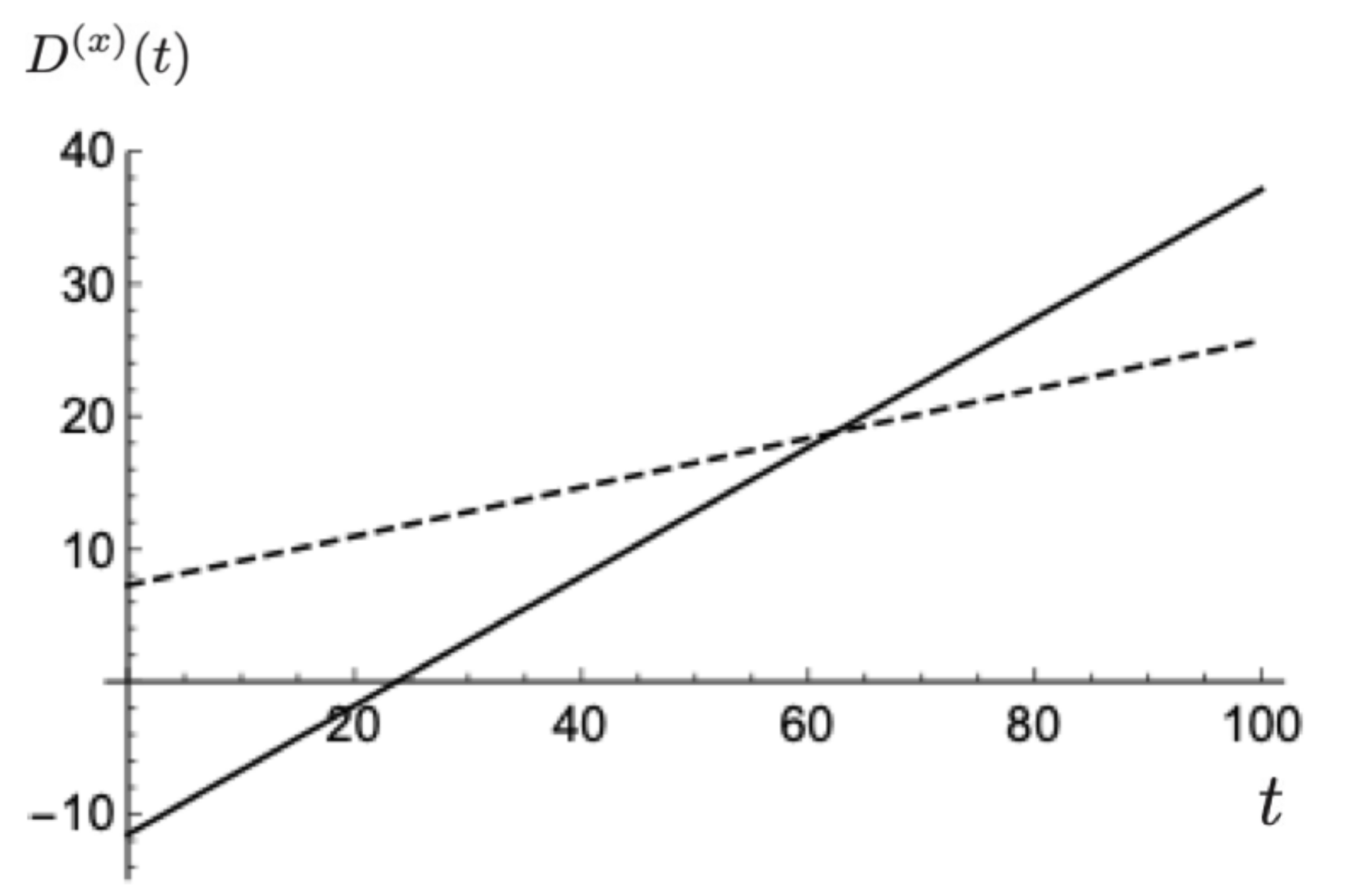
In
Figure 1, we display the time evolution of the phenomenological diffusion coefficient
under two different initial conditions. The constant term of the phenomenological diffusion coefficient
is given by
. This figure clearly shows that the constant term
can take a negative value depending on the initial conditions. Moreover,
increases linearly with time under both initial conditions, which is consistent with Equation (
3). The difference in the increase rate of
is due to the different initial distributions and thus the different variances of the sound velocity.
To draw this figure, we chose the positions of the two peaks of the Gaussian wave packet in the initial distribution as
for the solid-line with the negative constant term
and as
for the dashed-line with the positive constant term
. Note that we have chosen opposite signs for the momenta at the two peaks. These are the conditions for the two peaks to approach and to go away from each other, respectively (See Equation (
23)).
Therefore, the situation where apparent negative diffusion occurs with can be understood by the physical picture as follows. The width of each Gaussian distribution increases due to the diffusion process and the phase mixing process. Nevertheless, the width of the entire distribution function decreases because the two Gaussian distributions approach each other. As a result, the mean-square displacement decreases in the first stage of the time evolution. After the two Gaussian distributions pass each other, the variance of the displacement increases monotonically.
In
Figure 1, the value of
for the solid-line increases linearly with time and changes from negative to positive value around
. By drawing numerically the time evolution of the Wigner distribution function we confirmed that the two peaks of the Gaussian packets approach each other and pass around
.
We should note that the occurrence of the apparent negative diffusion is due to the approaching of the peaks in the initial distribution rather than due to the existence of the negative region in the Wigner distribution function.
We can say that the apparent negative diffusion occurs because of the competition between the effects of diffusion and phase mixing which leads to the approach of the two Gaussian wave packets. Because the phase mixing occurs due to the one-dimensionality of the system, this competition is unique to a 1D quantum system.
Even in the presence of the negative phase mixing process which reduces the mean-square displacement, there is no entropy reduction in this system since the phase mixing is a reversible process. On the contrary, the entropy in this system monotonically increases due to the diffusion process.


