
A New Analysis of Fractional-Order Equal-Width Equations via Novel Techniques
by
 , , , , and
Muhammad Naeem
1 ,
,
Ahmed M. Zidan
2,3,
Kamsing Nonlaopon
4,* ,
,
Muhammad I. Syam
5,
Zeyad Al-Zhour
6 and
Rasool Shah
7 1
Deanship of Joint First Year, Umm Al-Qura University, Makkah P.O. Box 517, Saudi Arabia
2
Department of Mathematics, College of Science, King Khalid University, Abha 9004, Saudi Arabia
3
Department of Mathematics, Faculty of Science, Al-Azhar University, Assiut 71524, Egypt
4
Department of Mathematics, Faculty of Science, Khon Kaen University, Khon Kaen 40002, Thailand
5
Department of Mathematical Sciences, United Arab Emirates University, Al Ain 15551, United Arab Emirates
6
Department of Basic Engineering Sciences, College of Engineering, Imam Abdulrahman Bin Faisal University, Dammam 31441, Saudi Arabia
7
Department of Mathematics, Abdul Wali Khan University, Mardan 23200, Pakistan
*
Author to whom correspondence should be addressed.
Symmetry 2021, 13(5), 886; https://0-doi-org.brum.beds.ac.uk/10.3390/sym13050886
Submission received: 27 April 2021
/
Revised: 7 May 2021
/
Accepted: 12 May 2021
/
Published: 17 May 2021
(This article belongs to the Special Issue Methods on Discrete Dynamical Systems, Networks, and Optimization for Signal Modelling)
Abstract
:In this paper, the new iterative transform method and the homotopy perturbation transform method was used to solve fractional-order Equal-Width equations with the help of Caputo-Fabrizio. This method combines the Laplace transform with the new iterative transform method and the homotopy perturbation method. The approximate results are calculated in the series form with easily computable components. The fractional Equal-Width equations play an essential role in describe hydromagnetic waves in cold plasma. Our object is to study the nonlinear behaviour of the plasma system and highlight the critical points. The techniques are very reliable, effective, and efficient, which can solve a wide range of problems arising in engineering and sciences.
1. Introduction
Many researchers have studied fractional evaluation equations in the last decade because of their significant applicability in various fields of modern technology and science. It has been demonstrated that time-fractional equations define certain physical processes and that their application solves different problems. In this regard, it is critical to develop more implementations of innovative for fractional calculus [1,2,3,4,5,6]. Ford and Simpson found the fractional Caputo derivative [7] to be the best technique for finding time-fractional problems since it consistently contains the initial specifications that are missing in different individual models [8]. According to Spanier and Oldham, integrals and fractional derivatives can be utilized to demonstrate much more useful synthetic models than traditional approaches [9]. Furthermore, later on, fractional theory commitments and implementation, such as fractal mathematics, can be discussed in the literature. Readers interested are referred to [10,11,12,13,14,15,16,17,18].
Many researchers have focused on partial differential equations in recent years due to their wide range of technology and research implementations. These fractional equations are appropriate for identifying different important inventions in fluid dynamics, magnetic fields, nuclear physics, acoustics, electrodynamics, particle physics, optical structures, viscoelasticity, and other fields [19,20,21]. The fractional-order nonlinear Equal-Width equations are fundamental partial differential equations that show the various complex nonlinear phenomenon in the field of sciences, usually in plasma physics, plasma waves, fluid mechanics, chemical physics, solid-state physics, etc. The Equal-Width equations described the behavior of nonlinear waves in a variety of nonlinear systems, including hydromagnetic waves in acoustic waves in plasma, surface waves incompressible fluids, cold plasma, shallow water waves, acoustic waves in enharmonic crystals, and so on [22,23,24,25].
The general fractional-order equal width (EW) equation has the following form for long waves traveling in the positive direction [26,27,28,29,30,31,32,33]:
where p is a positive integer; and are the positive constant, which require the boundary conditions as ; and is a parameter presenting order of fractional derivative. The derivative is understood in Caputo–Fabrizio form. Function is probability density function, is the spatial coordinate, and ℑ is the temporal coordinate. This expression carries a parameter that describes fractional-order derivative. For , fractional-order equations convert into classical equations. In this paper, we shall incorporate periodic boundary conditions for a region . The form of the initial wave will be taken so that at large distances from the wave, is very small and follows the free-space boundary conditions .
Numerous researchers have used various techniques to solve nonlinear fractional differential equations. Many investigators have used various methods to solve a variety of problems in previously implemented different analytical and numerical methods, such as the Adomian decomposition technique, finite difference method, generalized differential transform technique, finite element technique, perturbation methods, fractional differential transform technique, homotopy analysis strategy, iterative technique, etc., see [26,27,28,29,30,31,34,35,36] for more details. The homotopy analysis method (HAM) is a brilliant mathematical strategy proposed and applied by Liao [32,33,37]. Some scientists have shown the promise of using the HAM to study different mathematical modeling [38]. Furthermore, a good fundamental method identified as the homotopy analysis transform technique is as an important example of the homotopy analysis method that is used by combining the Laplace transformation technique. This inventive convergence of HAM and Laplace transformation is used to examine a wide variety of different problems [39,40]. When compared to traditional methods, these changes promote and strengthen the problem-solving methodology.
Several authors have suggested techniques for find the solution of fractional partial differential equations applying the fractional order Caputo and Fabrizio operators. The fractional-order wave equations was analyzed analytically by Xu in [41], who reduced the governing equation to two fractional ordinary differential equations. Dehghan et al. in [42], for example, used the HAM to solve linear partial differential equations; fractional derivatives are expressed by Liouville-Caputo sense in this work. Using the CF fractional derivative, Goufo et al. [43] developed a mathematical analysis of a model of rock fracture in the environment and achieved computational and analytical techniques. In [44], Jafari et al. utilized the HAM to solve a multi-order fractional differential equation investigated by Diethelm and Ford [45]. The chinese mathemation JH He introduce the homotopy perturbation method in 1998 [46]. This technique is efficient and accurate and eliminates an unconditione matrix, complicate integrals, and infinite series form. This method does not need of the problem a specific parameters. The homotopy perturbation transformation method (HPTM) combines the Elzaki transformation and the Homotopy perturbation method. Many researcher have been implemented HPTM to solving differential equations, such as Navier-Stokes problems [47], heat-like problems [48], gas dynamic model [49], Fisher’s and hyperbolic equation [50].
Daftardar-Gejji and Jafari [51,52] developed a new iterative approach for solving nonlinear equations in 2006. Jafari et al. [53] first applied Laplace transform in the iterative technique. They proposed a new straightforward method called the iterative Laplace transform method to look for the numerical solution of the fractional partial differential equation (FPDE) system. the iterative Laplace transform method to solve linear and non-linear partial differential equations such as time-fractional Fokker Planck equation [54], Zakharov Kuznetsov equation [55] and Fornberg Whitham equation [56], etc.
In this paper, we use the Iterative and homotopy perturbation transform methods to solved fractional Equal-Width equations with the help of Caputo-Fabrizio. The fractional calculus fundamental definitions are defined in Section 2, write the general methodologies in Section 3 and Section 4, many test models to show the effectiveness of suggested techniques are given in Section 5 and Section 6, and finally, the conclusion is given in Section 7.
2. Preliminaries Concepts
This section provides some fundamental concepts of fractional calculus.
Definition 1
([57]). The Liouville–Caputo fractional derivative of order ϱ is given as:
where is the integer n-th order derivative of and .
For , we defined the Laplace transform for the Liouville–Caputo fractional derivative of order ϱ as:
Definition 2
([57]). The Caputo–Fabrizio fractional derivative of order ϱ is defined by
where is a normalization form such that . The exponential law is used as the nonsingular kernel in this fractional derivative.
For , we defined the Laplace transform for the Caputo–Fabrizio fractional derivative of order ϱ as:
3. Homotopy Perturbation Transform Method
Consider the general form fractional-order partial differential equation of the form
with the initial condition
where is the fractional-order Caputo operator of and N are linear and nonlinear functions, and the source term is .
Next, we apply the Laplace transform to (5), and we get
Further, simplification through Laplace differentiation leads to
Now, the perturbation procedure in terms of power series with parameter p is presented as
where perturbation term is p and .
The nonlinear terms can be defined as
where are He’s polynomials of and can be determined as [46]
where
4. The New Iterative Transform Method Basic Procedure
Consider a particular type of a FPDE of the form
with the initial conditions
where M and N are linear and nonlinear functions, respectively.
5. Implementation of the HPTM
Example 1.
Consider the fractional-order nonlinear Equal-Width equation; if , and is given as
with the initial condition
Applying the Laplace transform to (29) with initial condition (30), we have
or
Now, using the inverse Laplace transform to (32), we have
Now, by implementing HPM, we get
The nonlinear terms can be defined with the help of He’s polynomials
He’s polynomials are defined as
With the coefficients comparing p-like, we get
and
Provided the series form solution is
Then, we have
Putting into (36), we obtain the solution of this problem as
The exact solution of this problem as follows:
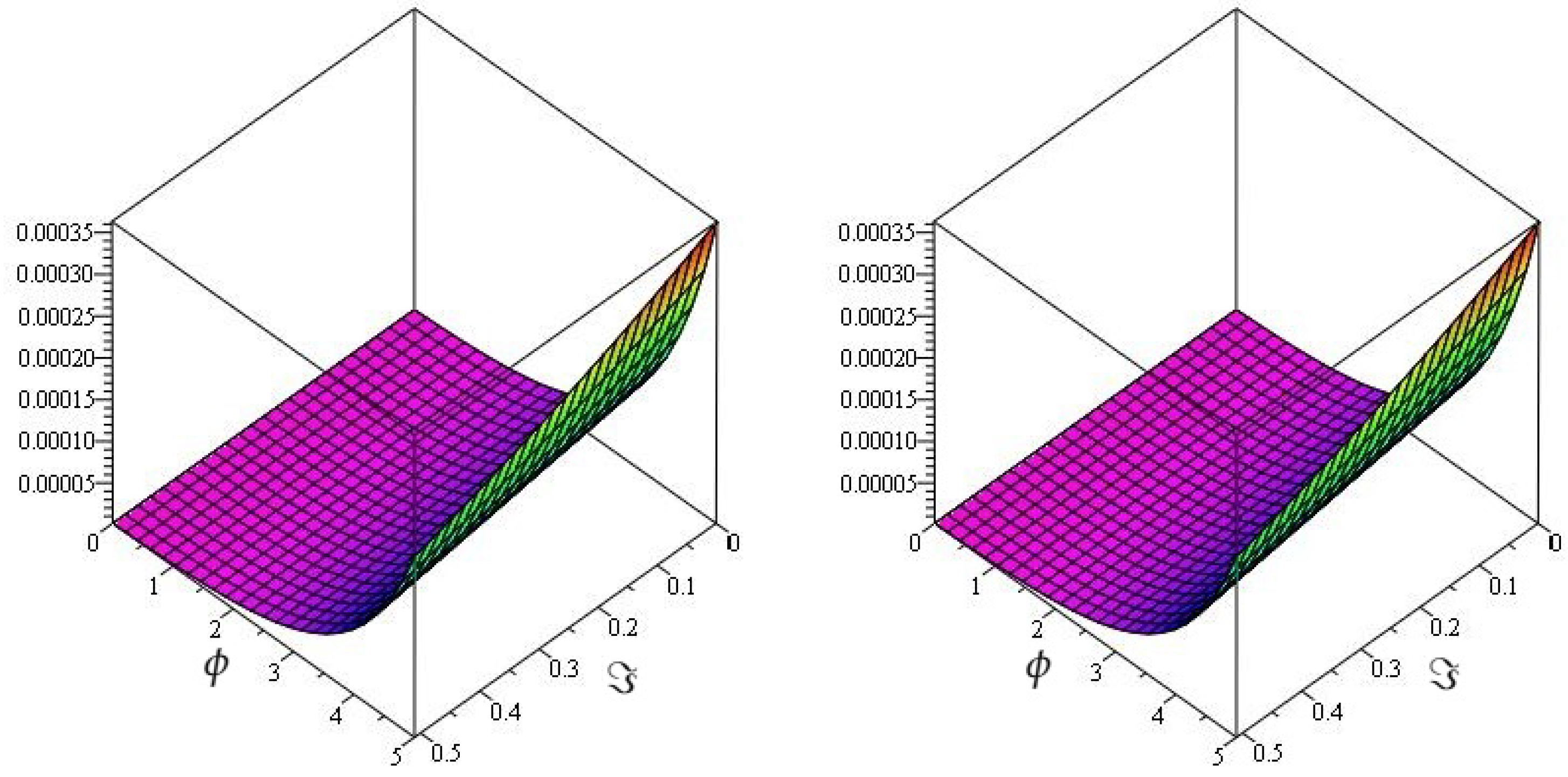
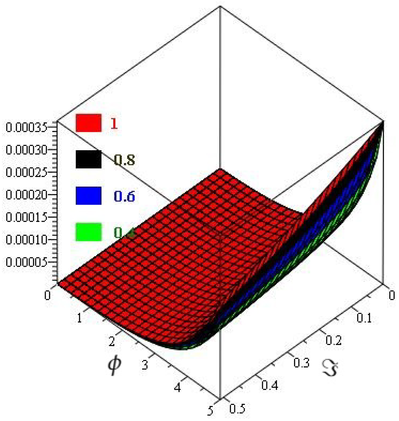
In Figure 1, the exact and the HPTM solutions of Example 1 at are shown by subgraphs. From the given figure, it can be seen that both the HPTM and exact results are in close contact with each other. Furthermore, in Figure 2, the HPTM results of Example 1 are investigated at different fractional-order at and of the 3D graph. It is analyzed that fractional-order problem solutions converge to an integer-order effect as fractional-order analysis to integer-order.
Example 2.
Consider the fractional nonlinear Equal-Width equation of the form: if , and are given as
with the initial condition
Applying Laplace transform to (39), we get
Using the initial condition (40) into (41), we get
By applying inverse Laplace transform to (42), we get
Now, we implement HPM, and we get
The nonlinear terms can be defined with the help of He’s polynomials
He’s polynomial are defined as
By comparing p-like coefficients, we get
The series form solution is
Then, we have
Putting in (46), we obtain the solution of this problem as
The exact solution of this problem is
In Figure 3, the exact and the HPTM solutions of Example 2 at are shown by subgraphs. From the given figure, it can be seen that both the HPTM and exact results are in close contact with each other. Furthermore, in Figure 4, the HPTM results of Example 2 are investigated at different fractional-order at and of 3D graph. According to the analysis, that fractional-order problem solutions converge to an integer-order effect as fractional-order analysis to integer-order.
Example 3.
Consider the fractional nonlinear fractional-order modified equal width equation is given as follows. Consider the fractional nonlinear Equal-Width equation of the form
with the initial condition
Using Laplace transform to (49), we get
Putting the initial condition (50) into (51), we have
By applying inverse Laplace transform to (52), we have
Now, we implement HPM, and we get
The nonlinear terms can be defined with the help of He’s polynomials
He’s polynomials are defined as
By comparing p-like coefficients, we get
The series form solution is
Then, we have
Putting into (56), we obtain the solution of this problem as
The exact solution of this problem is
In Figure 5, the exact and the HPTM solutions of Example 3 at are showm by subgraphs, respectively. From the given figure, it can be seen that both the HPTM and exact results are in close contact with each other. Furthermore, in Figure 6, the HPTM results of Example 3 are investigated at different fractional-order at and of 3D graph. Analysis shows that fractional-order problem solutions converge to an integer-order effect as fractional-order analysis to integer-order.
6. Implementation of Iterative Transform Method
Example 4.
Consider the fractional nonlinear Equal-Width equation of the form
with the initial condition
Applying the Laplace transform to (59), we get
Applying inverse Laplace transform to (61), we have
Now, by using the suggested analytical method, we get
The series form result is
Then, we have
Putting into (63), we obtain the solution of this problem as
The exact solution of this problem is
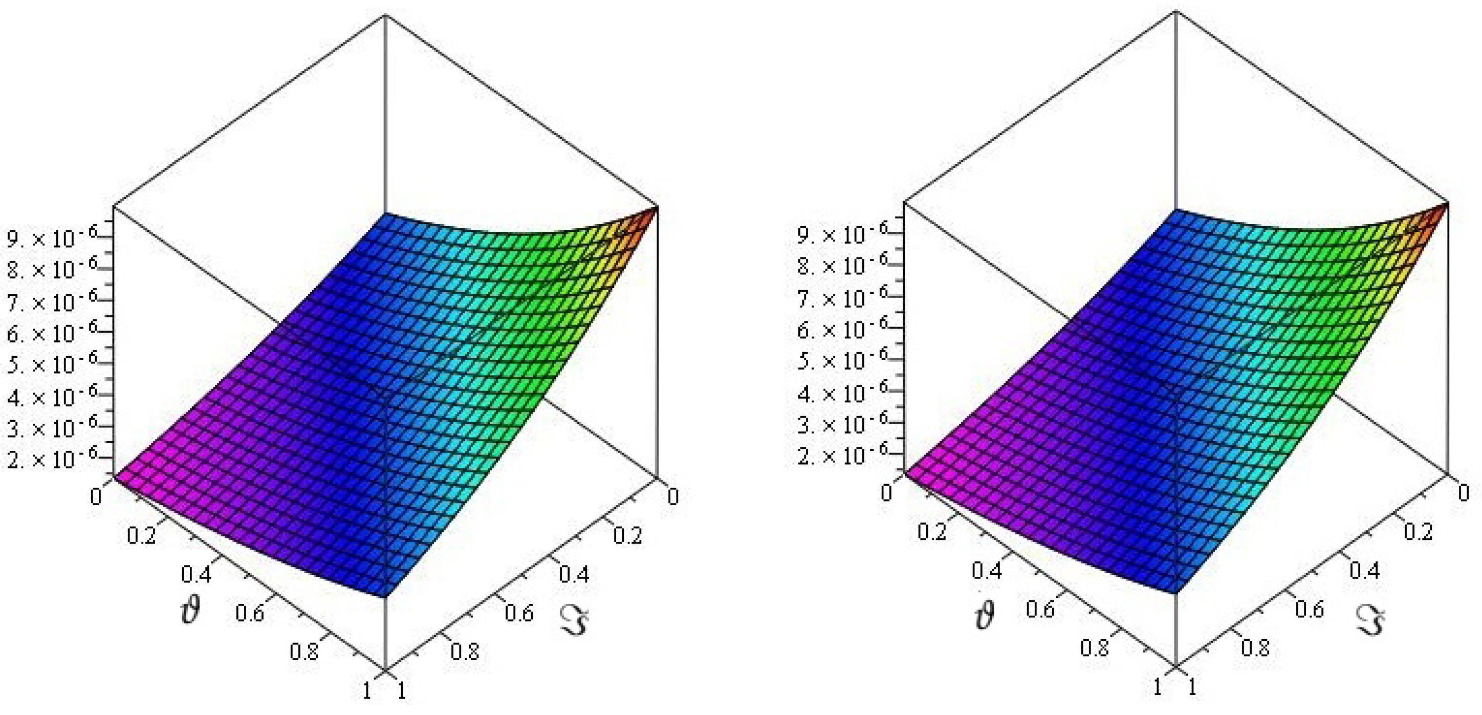
In Figure 7, it is shown that the exact and the NITM solutions graph with respect to ϕ and ℑ of Example 4 at . From the given figures, it can be seen that both the NITM and exact results are in close contact with each other. Furthermore, in Figure 8, the NITM results of Example 4 are investigated at different fractional-order at and of 2D graph with respect to ϕ and ℑ.
Example 5.
Consider the fractional nonlinear Equal-Width equation of the form
with the initial condition
Applying the Laplace transform to (66), we get
Applying inverse Laplace transform to (68), we have
Now, by using the suggested analytical method, we get
The series form result is
Then, we have
Putting into (70), we obtain the solution of this problem as
The exact solution of this problem is
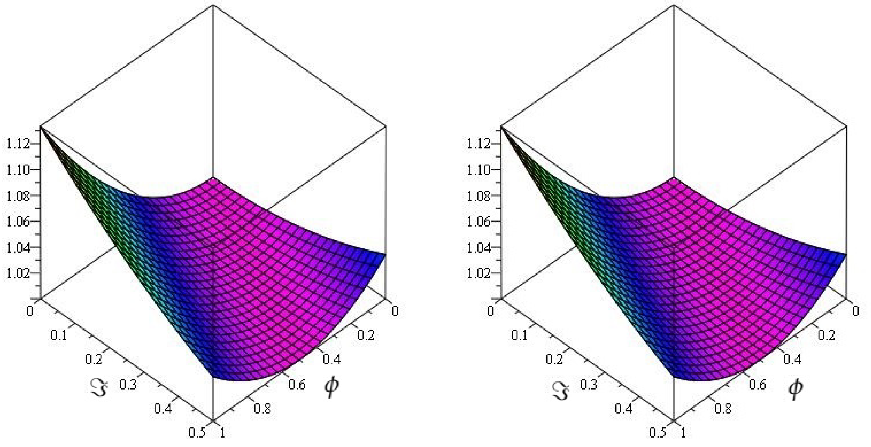
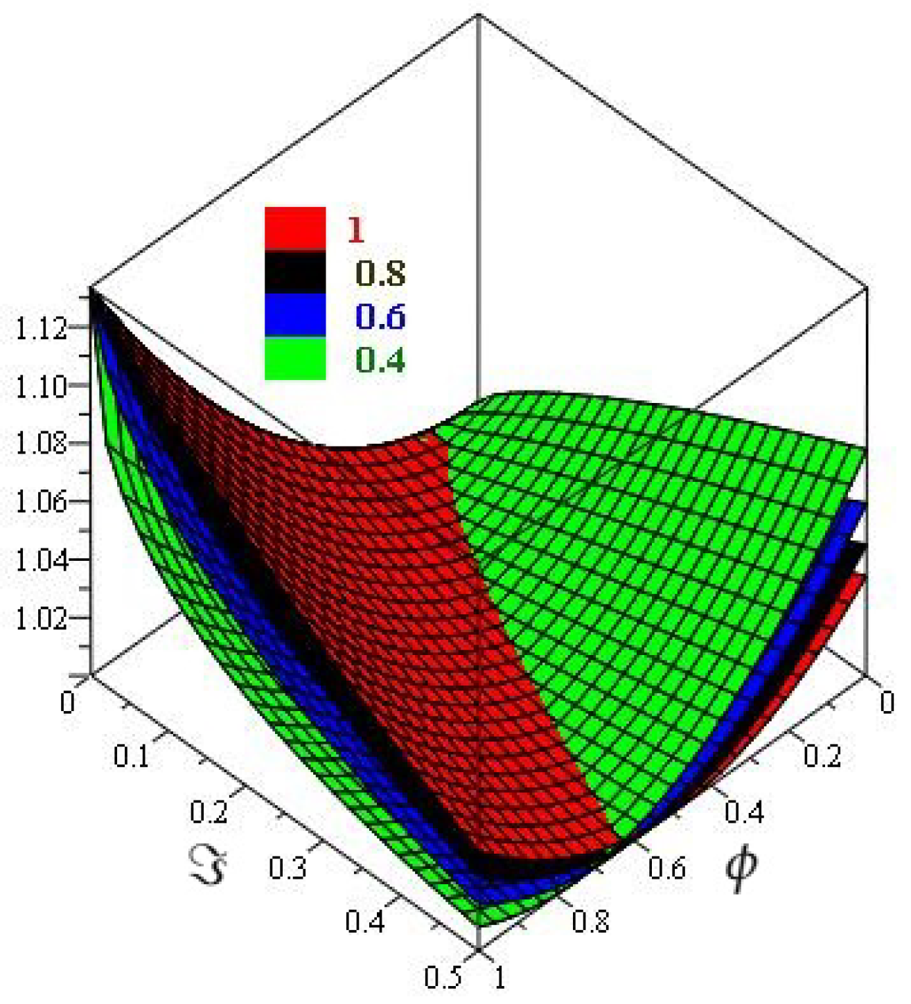
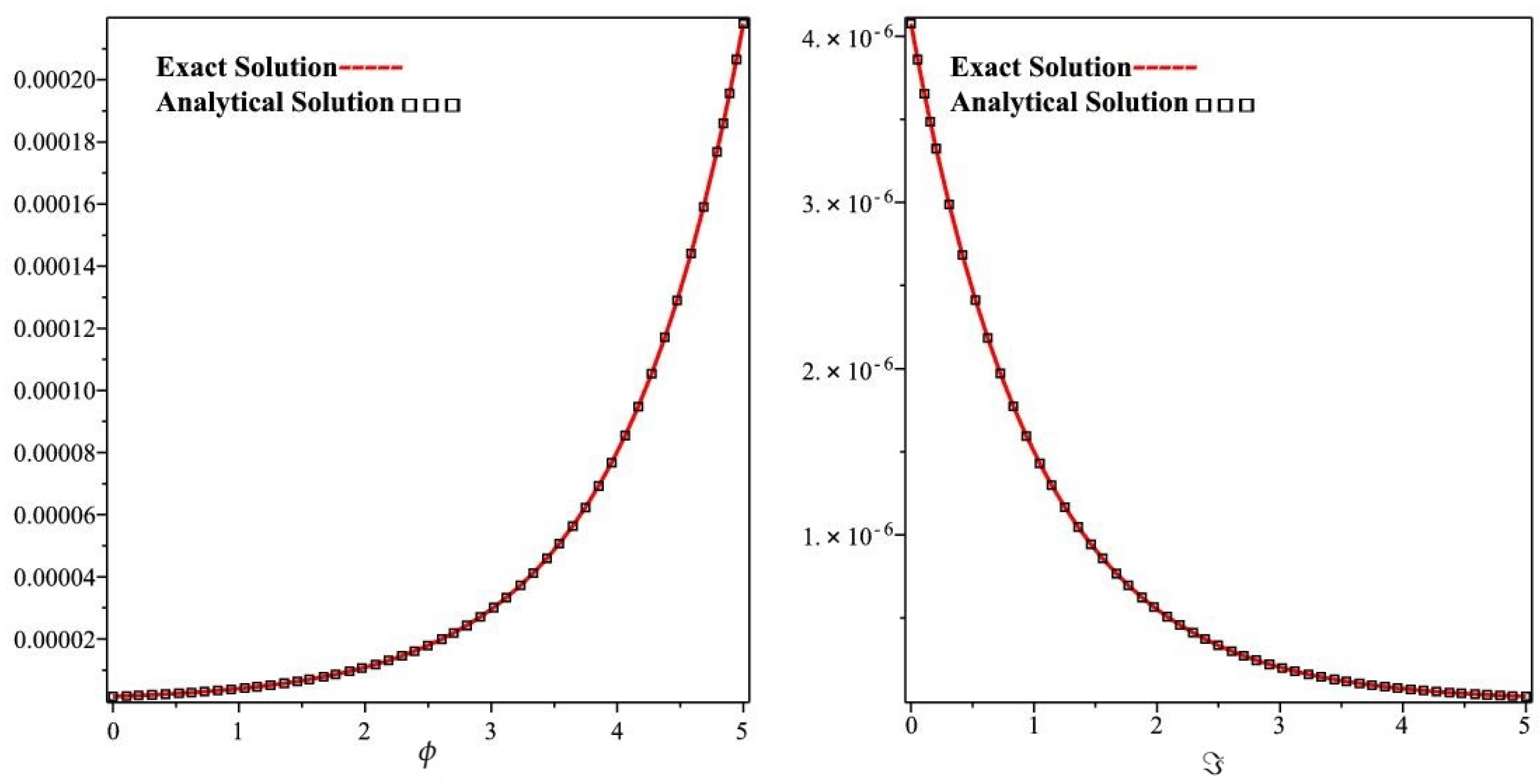
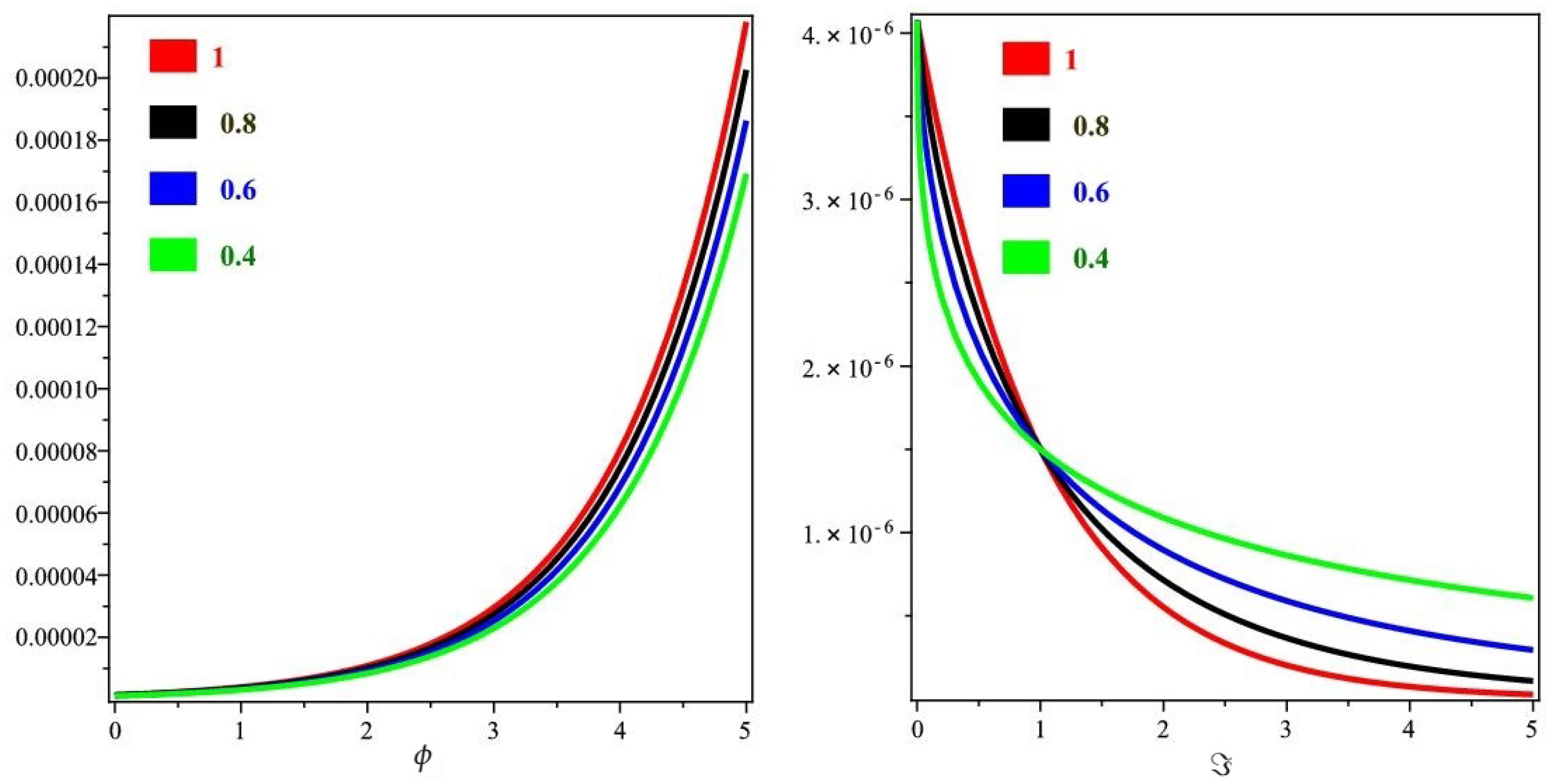
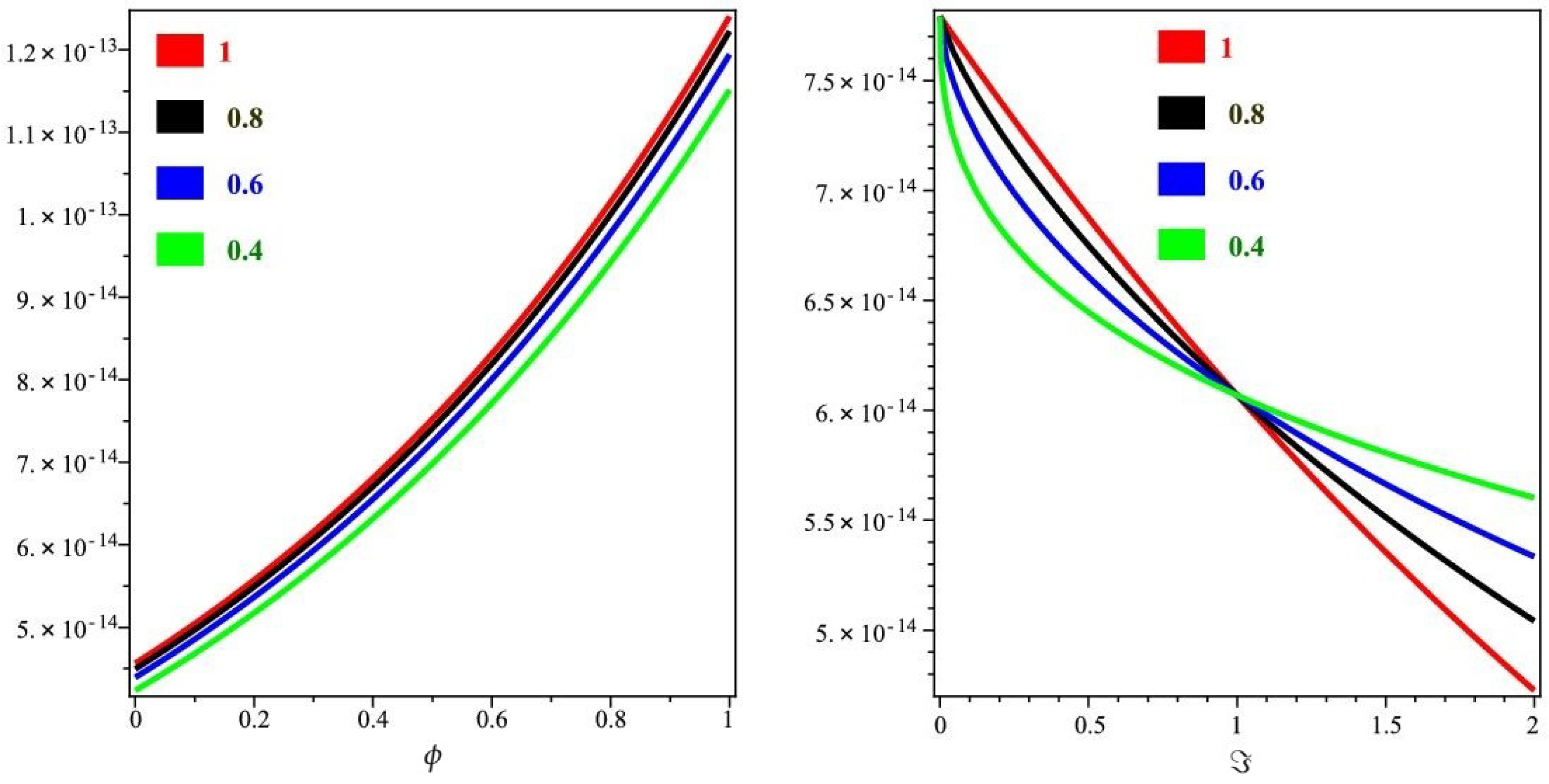
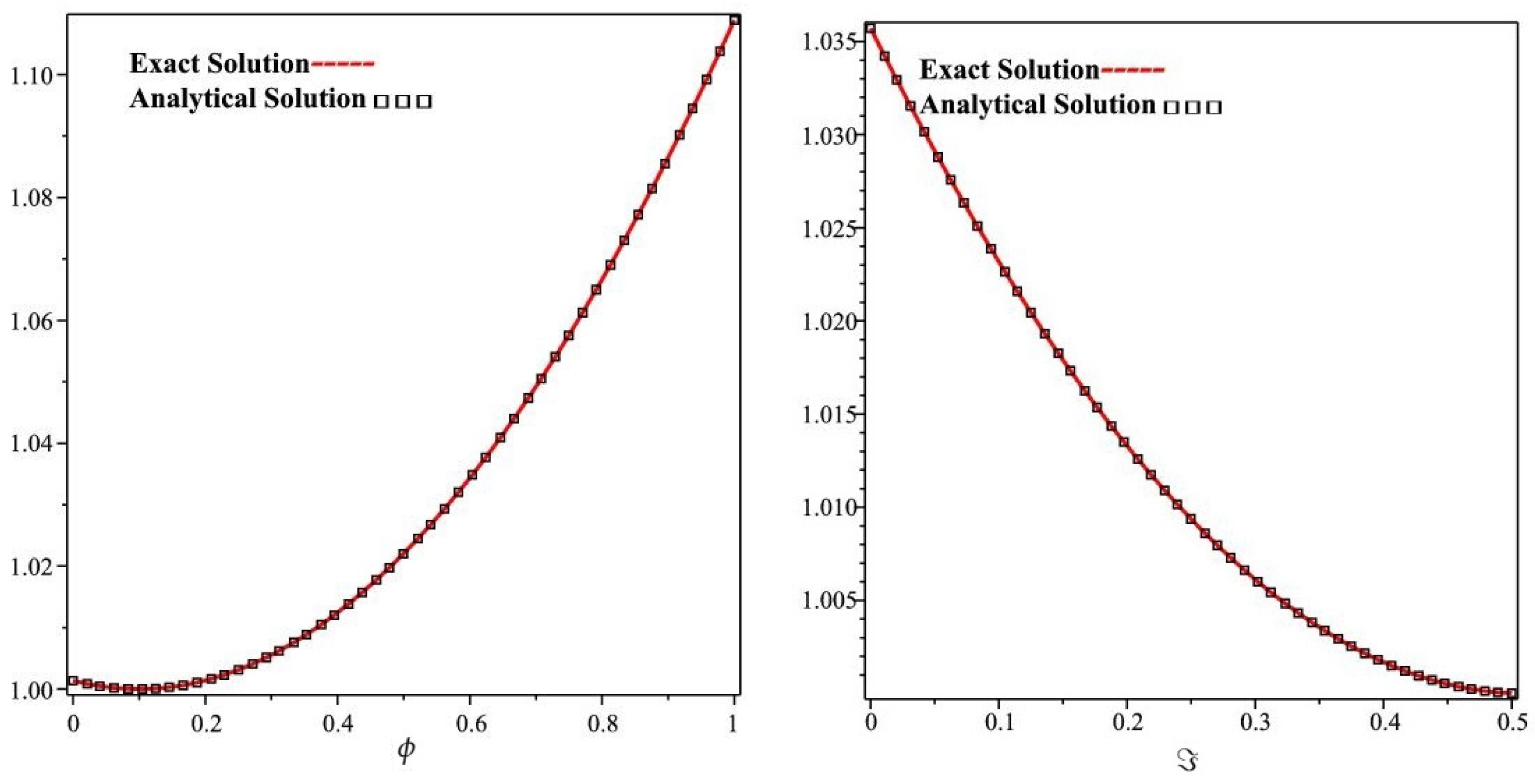
In Figure 9, it is shown that the exact and the NITM solutions graph with respect to ϕ and ℑ of Example 5 at . From the given figures, it can be seen that both the NITM and exact results are in close contact with each other. Furthermore, in Figure 10, the NITM results of Example 5 are investigated at different fractional-order at , and of 2D graph with respect to ϕ and ℑ.
Example 6.
Consider the fractional nonlinear Equal-Width equation of the form
with the initial condition
Applying the Laplace transform to (73), we get
Applying inverse Laplace transform to (75), we have
Now, by using the suggested analytical method, we get
The series form result is
Then, we have
Putting into (77), we obtain the solution of this problem as
The exact solution of this problem is
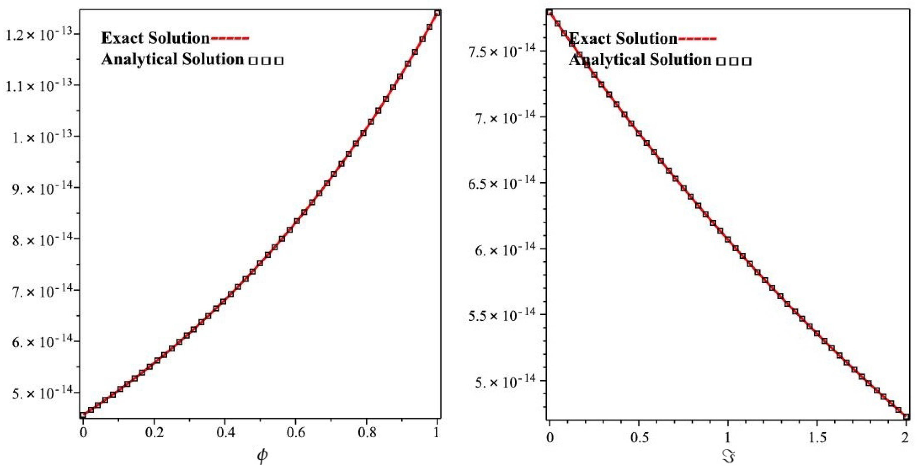
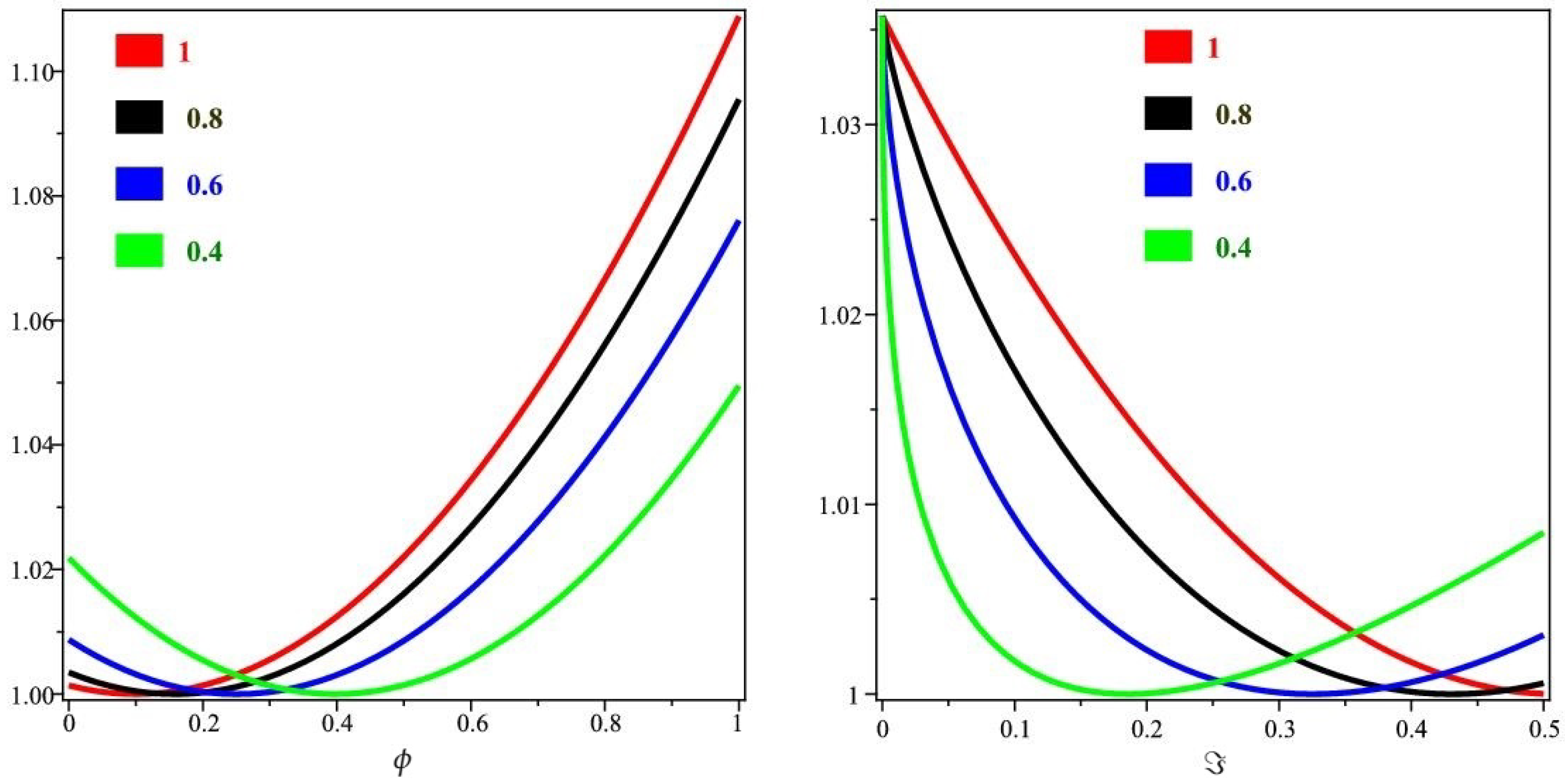
In Figure 11, it is shown that the exact and the NITM solutions graph with respect to ϕ and ℑ of Example 6 at . From the given figures, it can be seen that both the NITM and exact results are in close contact with each other. Furthermore, in Figure 12, the NITM results of Example 6 are investigated at different fractional-order at , and of the 2D graph with respect to ϕ and ℑ.
7. Conclusions
In this paper, we have presented a homotopy perturbation transform method and iterative transform method for solving fractional-order Equal-Width equations. The derivative is considered in the Caputo–Fabrizio sense. The figures analysis of the fractional-order results achieved has verified the convergence towards the results of the integer order. Finally, some examples have been shown to demonstrate the efficiency and accuracy of the current technique.
Author Contributions
Conceptualization, M.N., A.M.Z., K.N., M.I.S., Z.A.-Z. and R.S.; investigation, M.N., A.M.Z., K.N., M.I.S., M.N. and R.S.; methodology, M.N., A.M.Z., K.N., M.I.S., Z.A.-Z. and R.S.; validation, K.N., A.M.Z., M.N., Z.A.-Z. and R.S.; Formal Analysis, K.N., A.M.Z., M.I.S., Z.A.-Z. and R.S.; Resources, A.M.Z., M.I.S., Z.A.-Z. and R.S.; Data Curation, R.S.; Writing—Original Draft Preparation, K.N. and R.S.; Writing—Review and Editing, K.N. and R.S.; Project Administration, K.N.; Funding Acquisition, K.N. All authors have read and agreed to the published version of the manuscript.
Funding
One of the co-authors (A. M. Zidan) extends their appreciation to the Deanship of Scientific Research at King Khalid University, Abha 61413, Saudi Arabia, for funding this work through research groups program under grant number R.G.P.1/30/42.
Institutional Review Board Statement
Not applicable.
Informed Consent Statement
Not applicable.
Data Availability Statement
The numerical data used to support the findings of this study are included within the article.
Acknowledgments
The authors would like to thank the anonymous reviewers for their careful reading of our manuscript and their many insightful comments and suggestions, which helped us to improve the manuscript.
Conflicts of Interest
The authors declare no conflict of interest.
References
- Baleanu, D.; Guvenc, Z.B.; Machado, J.T. New Trends in Nanotechnology and Fractional Calculus Applications; Springer: New York, NY, USA, 2010. [Google Scholar]
- Baleanu, D.; Machado, J.A.; Luo, A.C. Fractional Dynamics and Control; Springer Science & Business Media: New York, NY, USA, 2011. [Google Scholar]
- Liu, Q.; Xu, Y.; Kurths, J. Active vibration suppression of a novel airfoil model with fractional order viscoelastic constitutive relationship. J. Sound Vib. 2018, 432, 50–64. [Google Scholar] [CrossRef]
- Xu, Y.; Li, Y.; Liu, D. A method to stochastic dynamical systems with strong nonlinearity and fractional damping. Nonlinear Dyn. 2016, 83, 2311–2321. [Google Scholar] [CrossRef]
- Xu, Y.; Li, Y.; Liu, D.; Jia, W.; Huang, H. Responses of Duffing oscillator with fractional damping and random phase. Nonlinear Dyn. 2013, 74, 745–753. [Google Scholar] [CrossRef]
- Saeed, T.; Ibrahim, A.; Marin, M. A GL model on thermo-elastic interaction in a poroelastic material using finite element method. Symmetry 2020, 3, 488. [Google Scholar] [CrossRef] [Green Version]
- Caputo, M. Linear models of dissipation whose Q is almost frequency independent II. Geophysics 1967, 13, 529–539. [Google Scholar] [CrossRef]
- Ford, N.J.; Simpson, A.C. The numerical solution of fractional differential equations: Speed versus accuracy. Numerai 2001, 26, 333–346. [Google Scholar]
- Oldham, K.B.; Spanier, J. The Fractional Calculus; Academic Press: New York, NY, USA, 1974. [Google Scholar]
- Ryzhkov, S.V.; Kuzenov, V.V. New realization method for calculating convective heat transfer near the hypersonic aircraft surface. Z. Angew. Math. Phys. 2019, 70, 1–9. [Google Scholar] [CrossRef]
- Caputo, M.; Fabrizio, M. A new definition of fractional derivative without singular kernel. Fract. Differ. Appl. 2015, 2, 731–785. [Google Scholar]
- Losada, J.; Nieto, J.J. Properties of the new fractional derivative without singular kernel. Fract. Differ. Appl. 2015, 2, 87–92. [Google Scholar]
- Yang, X.J.; Baleanu, D.; Srivastava, H.M. Local Fractional Integral Transforms and Their Applications; Academic Press: Cambridge, MA, USA, 2015. [Google Scholar]
- Baleanu, D.; Mustafa, O.G. On the global existence of solutions to a class of fractional differential equations. Comput. Math. Appl. 2010, 59, 35–41. [Google Scholar] [CrossRef] [Green Version]
- Yousef, F.; Alquran, M.; Jaradat, I.; Momani, S.; Baleanu, D. Ternary-fractional differential transform schema: Theory and application. Adv. Differ. Equ. 2019, 2019, 197. [Google Scholar] [CrossRef]
- Bokhari, A.; Baleanu, D.; Belgacem, R. Application of Shehu transform to Atangana-Baleanu derivatives. Int. J. Math. Comput. Sci. 2019, 20, 101–107. [Google Scholar] [CrossRef] [Green Version]
- He, J.H.; Ji, F.Y. Two-scale mathematics and fractional calculus for thermodynamics. Therm. Sci. 2019, 21, 2131–2133. [Google Scholar] [CrossRef]
- Wang, K.L.; Yao, S.W.; Yang, H.W. A fractal derivative model for snow’s thermal insulation property. Therm. Sci. 2019, 23, 2351–2354. [Google Scholar] [CrossRef]
- Kakutani, T.; Ono, H. Weak non-linear hydromagnetic waves in a cold collision-free plasma. J. Phys. Soc. Japan. 1969, 26, 1305–1318. [Google Scholar] [CrossRef]
- Yang, X.J.; Srivastava, H.M.; Machado, J.A. A new fractional derivative without singular kernel: Application to the modelling of the steady heat flow. Therm. Sci. 2016, 20, 753–756. [Google Scholar] [CrossRef]
- Yang, X.J. Fractional derivatives of constant and variable orders applied to anomalous relaxation models in heat-transfer problems. Therm. Sci. 2017, 21, 1161–1171. [Google Scholar] [CrossRef] [Green Version]
- Singh, J.; Kumar, D.; Kumar, S. A new fractional model of nonlinear shock wave equation arising in flow of gases. Nonlinear Eng. 2014, 3, 43–50. [Google Scholar] [CrossRef]
- Yang, X.J.; Machado, J.T. A new fractional operator of variable order: Application in the description of anomalous diffusion. Physica 2017, 481, 276–283. [Google Scholar] [CrossRef] [Green Version]
- Paolo, D.B.; Fattorusso, L.; Versaci, M. Electrostatic field in terms of geometric curvature in membrane MEMS devices. Comm. Appl. Ind. Math. 2017, 8, 165–184. [Google Scholar]
- Yong, L.; Wang, H.; Chen, X.; Yang, X.; You, Z.; Dong, S.; Gao, J. Shear property, high-temperature rheological performance and low-temperature flexibility of asphalt mastics modified with bio-oil. Constr. Build. Mater. 2018, 174, 30–37. [Google Scholar]
- Odibat, Z.; Momani, S.; Erturk, V.S. Generalized differential transform method: Application to differential equations of fractional order. Appl. Math. Comput. 2008, 197, 467–477. [Google Scholar] [CrossRef]
- Arikoglu, A.; Ozkol, I. Solution of fractional differential equations by using differential transform method. Chaos Solitons Fractals 2007, 34, 1473–1481. [Google Scholar] [CrossRef]
- Zhang, X.; Zhao, J.; Liu, J.; Tang, B. Homotopy perturbation method for two dimensional time-fractional wave equation. Appl. Math. Model. 2014, 38, 5545–5552. [Google Scholar] [CrossRef]
- Prakash, A. Analytical method for space-fractional telegraph equation by homotopy perturbation transform method. Nonlinear Eng. 2016, 5, 123–128. [Google Scholar] [CrossRef]
- Dhaigude, C.; Nikam, V. Solution of fractional partial differential equations using iterative method. Fract. Calc. Appl. Anal. 2012, 15, 684–699. [Google Scholar] [CrossRef]
- Safari, M.; Ganji, D.D.; Moslemi, M. Application of He’s variational iteration method and Adomian’s decomposition method to the fractional KdV-Burgers-Kuramoto equation. Comput. Math. Appl. 2009, 58, 2091–2097. [Google Scholar] [CrossRef] [Green Version]
- Liao, S.J. The Proposed Homotopy Analysis Technique for the Solution of Nonlinear Problems. Ph.D. Thesis, Shanghai Jiao Tong University, Shanghai, China, 1992. [Google Scholar]
- Liao, S. Homotopy analysis method: A new analytical technique for nonlinear problems. Comm. Nonlinear Sci. Numer. Simulat. 1997, 2, 95–100. [Google Scholar] [CrossRef]
- Meerschaert, M.M.; Tadjeran, C. Finite difference approximations for two-sided space-fractional partial differential equations. Appl. Numer. Math. 2006, 56, 80–90. [Google Scholar] [CrossRef]
- Ray, S.S.; Bera, R.K. Analytical solution of the Bagley Torvik equation by Adomian decomposition method. Appl. Math. Comput. 2005, 168, 398–410. [Google Scholar] [CrossRef]
- Jiang, Y.; Ma, J. High-order finite element methods for time-fractional partial differential equations. J. Comput. Appl. Math. 2011, 235, 3285–3290. [Google Scholar] [CrossRef] [Green Version]
- Liao, S. On the homotopy analysis method for nonlinear problems. Appl. Math. Comput. 2004, 147, 499–513. [Google Scholar] [CrossRef]
- Abbasbandy, S.; Hashemi, M.S.; Hashim, I. On convergence of homotopy analysis method and its application to fractional integro-differential equations. Quaest. Math. 2013, 36, 93–105. [Google Scholar] [CrossRef]
- Kumar, D.; Singh, J.; Baleanu, D. A fractional model of convective radial fins with temperature-dependent thermal conductivity. Rom. Rep. Phys. 2017, 69, 103. [Google Scholar]
- Kumar, D.; Agarwal, R.P.; Singh, J. A modified numerical scheme and convergence analysis for fractional model of Lienards equation. J. Comput. Appl. Math. 2018, 339, 405–413. [Google Scholar] [CrossRef]
- Hang, X.; Jie Cang, J. Analysis of a time fractional wave-like equation with the homotopy analysis method. Phys. Lett. A 2008, 372, 1250–1255. [Google Scholar]
- Dehghan, M.; Manafian, J.; Saadatmandi, A. The solution of the linear fractional partial differential equations using the homotopy analysis method. Z. Naturforsch. A 2010, 65, 935–949. [Google Scholar] [CrossRef] [Green Version]
- Goufo, E.F.D.; Pene, M.K.; Mwambakana, J.N. Duplication in a model of rock fracture with fractional derivative without singular kernel. Open Math. 2015, 13, 839–846. [Google Scholar] [CrossRef] [Green Version]
- Jafari, H.; Das, S.; Tajadodi, H. Solving a multi-order fractional differential equation using homotopy analysis method. J. King Saud Univ. Sci. 2011, 23, 151–155. [Google Scholar] [CrossRef] [Green Version]
- Diethelm, K.; Ford, N.J. Multi-order fractional differential equations and their numerical solution. Appl. Math. Comput. 2004, 154, 621–640. [Google Scholar] [CrossRef]
- He, J.H. Homotopy perturbation method: A new nonlinear analytical technique. Appl. Math. Comput. 2003, 135, 73–79. [Google Scholar] [CrossRef]
- Jena, R.; Chakraverty, S. Solving time-fractional Navier–Stokes equations using homotopy perturbation Elzaki transform. SN Appl. Sci. 2018, 1, 16. [Google Scholar] [CrossRef] [Green Version]
- Mahgoub, M.; Sedeeg, A. A comparative study for solving nonlinear fractional heat-like equations via Elzaki transform. Br. J. Math. Comp. Sci. 2016, 19, 1–12. [Google Scholar] [CrossRef]
- Das, S.; Gupta, P. An approximate analytical solution of the fractional diffusion equation with absorbent term and external force by homotopy perturbation method. Z. Naturforsch. 2010, 65, 182–190. [Google Scholar] [CrossRef]
- Singh, P.; Sharma, D. Comparative study of homotopy perturbation transformation with homotopy perturbation Elzaki transform method for solving nonlinear fractional PDE. Nonlinear Eng. 2019, 9, 60–71. [Google Scholar] [CrossRef]
- Daftardar-Gejji, V.; Jafari, H. An iterative method for solving nonlinear functional equations. J. Math. Anal. Appl. 2006, 316, 753–763. [Google Scholar] [CrossRef] [Green Version]
- Jafari, H.; Khalique, C.M.; Nazari, M. Application of the Laplace decomposition method for solving linear and nonlinear fractional diffusion-wave equations. Appl. Math. Lett. 2011, 24, 1799–1805. [Google Scholar] [CrossRef] [Green Version]
- Jafari, H.; Nazari, M.; Baleanu, D.; Khalique, C.M. A new approach for solving a system of fractional partial differential equations. Comput. Math. Appl. 2013, 66, 838–843. [Google Scholar] [CrossRef]
- Yan, L. Numerical solutions of fractional Fokker-Planck equations using iterative Laplace transform method. Abstr. Appl. Anal. 2013, 2013, 465160. [Google Scholar] [CrossRef]
- Prakash, A.; Kumar, M.; Baleanu, D. A new iterative technique for a fractional model of nonlinear Zakharov-Kuznetsov equations via Sumudu transform. Appl. Math. Comput. 2018, 334, 30–40. [Google Scholar] [CrossRef]
- Ramadan, M.A.; Al-luhaibi, M.S. New iterative method for solving the Fornberg-Whitham equation and comparison with homotopy perturbation transform method. Br. J. Math. Comp. Sci. 2014, 4, 1213–1227. [Google Scholar] [CrossRef]
- Morales-Delgado, V.F.; Gomez-Aguilar, J.F.; Yepez-Martinez, H.; Baleanu, D.; Escobar-Jimenez, R.F.; Olivares-Peregrino, V.H. Laplace homotopy analysis method for solving linear partial differential equations using a fractional derivative with and without kernel singular. Adv. Differ. Equ. 2016, 2016, 1–17. [Google Scholar] [CrossRef] [Green Version]
Figure 1.
The actual and HPTM solution graphs at of Example 1.

Figure 2.
The HPTM solution of different fractional-order ϱ graph of Example 1.

Figure 3.
The actual and HPTM solution graphs at of Example 2.

Figure 4.
The HPTM solution of different fractional-order ϱ graph of Example 2.

Figure 5.
The actual and HPTM solution graphs at of Example 3.

Figure 6.
The HPTM solution of different fractional-order ϱ graph of Example 3.

Figure 7.
The actual and ITM solution graphs at with respect to ϕ and ℑ of Example 4.

Figure 8.
The ITM solution of different fractional-order ϱ graphs with respect to ϕ and ℑ of Example 4.
Figure 8.
The ITM solution of different fractional-order ϱ graphs with respect to ϕ and ℑ of Example 4.

Figure 9.
The actual and ITM solution graphs at with respect to ϕ and ℑ of Example 5.

Figure 10.
The ITM solution of different fractional-order ϱ graphs with respect to ϕ and ℑ of Example 5.
Figure 10.
The ITM solution of different fractional-order ϱ graphs with respect to ϕ and ℑ of Example 5.

Figure 11.
The actual and ITM solution graphs at with respect to ϕ and ℑ of Example 6.

Figure 12.
The ITM solution of different fractional-order ϱ graphs with respect to ϕ and ℑ of Example 6.
Figure 12.
The ITM solution of different fractional-order ϱ graphs with respect to ϕ and ℑ of Example 6.

Publisher’s Note: MDPI stays neutral with regard to jurisdictional claims in published maps and institutional affiliations. |
© 2021 by the authors. Licensee MDPI, Basel, Switzerland. This article is an open access article distributed under the terms and conditions of the Creative Commons Attribution (CC BY) license (https://creativecommons.org/licenses/by/4.0/).
Share and Cite
MDPI and ACS Style
Naeem, M.; Zidan, A.M.; Nonlaopon, K.; Syam, M.I.; Al-Zhour, Z.; Shah, R. A New Analysis of Fractional-Order Equal-Width Equations via Novel Techniques. Symmetry 2021, 13, 886. https://0-doi-org.brum.beds.ac.uk/10.3390/sym13050886
AMA Style
Naeem M, Zidan AM, Nonlaopon K, Syam MI, Al-Zhour Z, Shah R. A New Analysis of Fractional-Order Equal-Width Equations via Novel Techniques. Symmetry. 2021; 13(5):886. https://0-doi-org.brum.beds.ac.uk/10.3390/sym13050886
Chicago/Turabian StyleNaeem, Muhammad, Ahmed M. Zidan, Kamsing Nonlaopon, Muhammad I. Syam, Zeyad Al-Zhour, and Rasool Shah. 2021. "A New Analysis of Fractional-Order Equal-Width Equations via Novel Techniques" Symmetry 13, no. 5: 886. https://0-doi-org.brum.beds.ac.uk/10.3390/sym13050886
Note that from the first issue of 2016, this journal uses article numbers instead of page numbers. See further details here.