
A Topology Optimization Method Based on Non-Uniform Rational Basis Spline Hyper-Surfaces for Heat Conduction Problems


Arts et Métiers Institute of Technology, Université de Bordeaux, CNRS, INRA, Bordeaux INP, HESAM Université, I2M UMR 5295, F-33405 Talence, France
*
Author to whom correspondence should be addressed.
Symmetry 2021, 13(5), 888; https://0-doi-org.brum.beds.ac.uk/10.3390/sym13050888
Submission received: 17 April 2021
/
Revised: 7 May 2021
/
Accepted: 12 May 2021
/
Published: 17 May 2021
(This article belongs to the Special Issue Mathematical Theory, Methods, and Its Applications for Industry)
Abstract
:This work deals with heat conduction problems formulation in the framework of a CAD-compatible topology optimization method based on a pseudo-density field as a topology descriptor. In particular, the proposed strategy relies, on the one hand, on the use of CAD-compatible Non-Uniform Rational Basis Spline (NURBS) hyper-surfaces to represent the pseudo-density field and, on the other hand, on the well-known Solid Isotropic Material with Penalization (SIMP) approach. The resulting method is then referred to as NURBS-based SIMP method. In this background, heat conduction problems have been reformulated by taking advantage of the properties of the NURBS entities. The influence of the integer parameters, involved in the definition of the NURBS hyper-surface, on the optimized topology is investigated. Furthermore, symmetry constraints, as well as a manufacturing requirement related to the minimum allowable size, are also integrated into the problem formulation without introducing explicit constraint functions, thanks to the NURBS blending functions properties. Finally, since the topological variable is represented by means of a NURBS entity, the geometrical representation of the boundary of the topology is available at each iteration of the optimization process and its reconstruction becomes a straightforward task. The effectiveness of the NURBS-based SIMP method is shown on 2D and 3D benchmark problems taken from the literature.
1. Introduction
The continuous downscaling of semi-conductor electronics in devices like smartphones and laptops, which require increasing power rates that need to be dissipated, calls for major challenges to design dedicated cooling systems [1]. Efficient heat transfer in electronic devices is of paramount importance because it allows operation at higher performance for longer duration [2]. Moreover, the performance of other devices, like heat exchangers, turbine blades, fins, thermoelectric generators, and cooling systems, critically depends on effective heat transfer [3,4,5,6,7]. Improved heat transfer design can reduce the energy consumption of devices during their operative life, thus allowing for a reduction of the operational costs. The use of dedicated optimization strategies in heat transfer problems can be also applied to increase the efficiency of support structures in various additive manufacturing technologies to save material and to allow producing more compact and cost-effective structures [8].
In the last decade, the use of topology optimization (TO) methods has experienced a significant growth in many industrial fields due also to the development of modern additive manufacturing processes. The goal of TO is to determine the optimal distribution of the material within a given design domain under prescribed requirements. Since its introduction in the late 1980s [9], numerous aproaches have been proposed in the literature [10,11], as the homogenization method [9,12], Solid Isotropic Material with Penalization (SIMP) method [10,13], Level Set Method (LSM) [14,15], Moving Morphable Components (MMC) method [16], Evolutionary Structural Optimization (ESO) method [17], and its improved version, i.e., the Bi-directional ESO [18,19] method.
TO has been extensively used in heat transfer problems [20,21,22,23,24,25,26,27]. An exhaustive review on this topic can be found in [28]. Li et al. [20,21] extend the ESO algorithm to shape optimization problems dealing with steady-state heat conduction. Zhuang et al. [22] employed the LSM to deal with TO heat conduction problems under multiple load cases. Yoon [23] proposed a formulation taking into account for forced convective heat transfer. In this background, the heat transfer equation with forced convective heat loss and the Navier-Stokes equation were integrated in the TO problem formulation. As a consequence, four material properties were interpolated in terms of the pseudo-density field: the inverse permeability, the conductivity, the material density, and the specific heat capacity. Iga et al. [27] focused on the influence of design-dependent heat convection coefficients and internal heat generation on the optimized topologies found by means of the homogenization method [29]. The dependency of these coefficients on the design variables was determined through a dedicated surrogate model. Ikonen et al. [24] formulated heat conduction problems in the framework of an interesting TO method based on parametric L-systems and the finite volume method (FVM). Results were compared to those provided by the classical SIMP approach showing equivalent or superior performances. Recently, Yoon and Koo [26] developed a sensitivity analysis for TO of steady-state conductive thermal problems subject to design-dependent thermal loads using density gradients–based boundary detection, whilst Hu et al. [25] presented an interesting application of TO dealing with heat transfer problems in microchannels in order to optimize their performances in terms of both heat dissipation and pressure drop. Bendsøe and Sigmund in [10] discussed the generalization of the well-known 99-line Matlab code to heat conduction problems.
It is noteworthy that the success of the SIMP method is due to its efficiency and compactness [10]. However, two major drawbacks affect such an approach. Firstly, the topological descriptor relies on the mesh of the finite element (FE) model, and it is not possible to obtain an optimized topology compatible with CAD software: accordingly, the results of the TO require a time-consuming CAD reconstruction/reassembly phase in order to integrate the optimized solution within the CAD environment. Secondly, to avoid the well-known checker-board effect, dedicated filtering techniques [10] or projection methods [30,31] must be introduced, which represent a further limitation of this method.
In order to overcome the aforementioned issues, the classical SIMP approach has been recently reformulated in the framework of Non-Uniform Rational Basis Spline hyper-surfaces [32,33,34,35,36,37,38,39]. The resulting method is then referred to as NURBS-based SIMP method. As discussed in [32,33], some consequences of outstanding importance result from this approach: (1) the number of design variables is unrelated to the number of elements and a significant reduction of the design variables amount can be obtained with respect to the classical SIMP approach; (2) the optimized topology is unrelated to the quality of the mesh of the FE model; (3) the NURBS formalism allows taking advantage of an implicitly defined filter zone, whose size depends on the NURBS parameters. Moreover, the CAD reconstruction phase is a trivial task [38], and, thanks to the peculiar features of the NURBS entities, it is possible to meet the design requirements on the reassembled geometry.
In this study, only heat conduction problems are considered, wherein the so-called thermal compliance is considered as a measure of the overall structural thermal conductivity. Heat conduction problems are formulated in the context of the NURBS-based SIMP method. The contribution of this study is twofold. Firstly, the gradient of thermal responses with respect to the topological variables is derived by exploiting the main properties of NURBS entities. In particular, the formulation benefits from the local support property of the NURBS blending functions [32,33], which establishes an implicit relation among the pseudo-densities of adjacent elements. Secondly, a sensitivity analysis of the optimized topology to the integer parameters of the NURBS entity is carried out. Particularly, these parameters can be set to define a minimum member size requirement without introducing an explicit constraint into the problem formulation, as discussed in [35]. The effectiveness of the NURBS-based SIMP method is tested on both 2D and 3D test cases taken from the literature.
The paper follows this outline. Section 2 presents the fundamentals of NURBS hyper-surfaces. Section 3 introduces the main concepts at the basis of the NURBS-based SIMP method. The numerical results are presented and discussed in Section 4: the differences obtained in the optimized topologies when using either B-spline or NURBS entities as topology descriptor are highlighted and the influence of the integer parameters involved in the definition of the NURBS entity is also investigated. Finally, meaningful conclusions and prospects are provided in Section 5.
Notation 1.
Upper-case bold letters are used to indicate tensors and matrices, while lower-case bold letters indicate column vectors.
2. Fundamentals of NURBS Hyper-Surfaces
A NURBS hyper-surface is a polynomial-based function, defined over a parametric space (domain), taking values in the NURBS space (co-domain). Therefore, if N is the dimension of the parametric space and M is the dimension of the NURBS space, a NURBS entity is defined as . The mathematical formula of a generic NURBS hyper-surface is
where () is the number of control points (CPs) along the parametric direction, are the piece-wise rational basis functions, which are related to the standard NURBS blending functions , by means of the relationship
In Equations (1) and (2), is a M-dimension vector-valued rational function, are scalar dimensionless parameters defined in the interval , whilst are the CPs coordinates. The j-th CP coordinate () is stored in the array , whose dimensions are . The explicit expression of CPs coordinates in is:
Curves and surfaces formulæ can be easily deduced from Equation (1). The CPs layout is referred to as control polygon for NURBS curves, control net for surfaces and control hyper-net otherwise [32]. The overall number of CPs constituting the hyper-net is:
The generic CP does not actually belong to the NURBS entity but it affects its shape by means of its coordinates. A weight is associated to the generic CP. The higher the weight , the more the NURBS entity is attracted towards the CP . For each parametric direction , , the NURBS blending functions are of degree and can be computed in a recursive way as
where each blending function is defined on the knot vector
whose dimension is , with
Each knot vector is a non-decreasing sequence of real numbers that can be interpreted as a discrete collection of values of the related dimensionless parameter . The NURBS blending functions are characterized by several interesting properties: the interested reader is referred to [40] for a deeper insight into the matter. Here, only the local support property is recalled because it is of paramount importance for the NURBS-based SIMP method [32,33]:
Equation (9) means that each CP (and the respective weight) affects only a precise zone of the parametric space, which is referred to as local support or influence zone.
3. The NURBS-Based SIMP Method
The details of the formulation of the SIMP method in the NURBS hyper-surfaces framework are given in [32,33]. The main features of the NURBS-based SIMP method for TO are briefly recalled here. The mathematical formulation is here provided for 3D steady-state heat conduction problems under the hypothesis that the applied thermal loads and boundary conditions (BCs) do not depend upon the pseudo-density field (of course, the formulation can be generalized by relaxing this hypothesis). Consider the compact space in a Cartesian orthonormal frame :
where () is a reference length defined along axis. The aim of TO is to search for the best distribution of a given “heterogeneous material” satisfying the requirements of the design problem.
Consider the steady-state equation of the FE model in the most general case:
where represents the overall number of degrees of freedom (DOFs) before applying the BCs, and is the non-reduced (singular) conductivity matrix of the FE model, while and are the non-reduced vectors of the external generalized nodal thermal forces and temperatures, respectively. Using standard FE notation [41], Equation (11) can be rewritten as:
with:
where represents the number of DOFs where temperature is imposed (Dirichlet’s BC), while is the number of unknown DOFs. In Equation (12), and are the unknown and imposed vectors of nodal temperatures, respectively. is the vector of generalized external nodal thermal forces, whilst is the vector of (unknown) generalized nodal thermal reactions at nodes where BCs are imposed.
, , and are the conductivity matrices of the FE model after applying BCs. Consider, now, the case of zero Dirichlet’s BCs and non-zero Neumann’s BCs: the thermal compliance of the structure is defined as:
In the SIMP approach, the material domain is identified by means of a pseudo-density function for : denotes absence of material, whilst indicates completely dense bulk material. The density field affects the element conductivity matrix and, accordingly, the global conductivity matrix of the FE model as
where is the fictitious density computed at the centroid of the generic element e, whilst is a parameter penalizing the intermediate densities between 0 and 1, in agreement with the classic SIMP approach ( in this study). is the total number of elements and is the number of DOFs of the generic element. In Equation (15), and are the non-penalized and the penalized conductivity matrices of element e, expressed in the global reference frame of the FE model, whilst is the connectivity matrix of element e.
In the context of the NURBS-based SIMP method, the pseudo-density field for a TO problem of dimension D is represented through a NURBS hyper-surface of dimension . Therefore, for a 3D problem a 4D entity is needed and the pseudo-density field reads:
In Equation (16), is the total number of CPs, constitutes the fourth coordinate of the array of Equation (1), while are the NURBS rational basis functions of Equation (2). The dimensionless parameter can be related to the Cartesian coordinates as follows:
Among the parameters tuning the shape of the NURBS entity, only the pseudo-density at CPs and the associated weights are identified as design variables and are collected in the vectors and , respectively, defined as:
The dimension of these arrays is equal to . Accordingly, in the most general case, the overall number of design variables is . Thus, the classic TO problem of thermal compliance minimization subject to an inequality constraint on the volume can be formulated as:
In Equation (19), is a reference volume, V is the volume of the material domain , while is the fixed volume fraction; is the volume of element e, and represents the lower bound, imposed to the density field to prevent any singularity for the solution of the equilibrium problem. The objective function is divided by a reference compliance, , to obtain a dimensionless value. The volume of the material domain appearing in Equation (19) is defined as:
where is the volume of element e. Moreover, in Equation (19), the linear index k has been introduced for the sake of compactness. The relationship between k and , () is:
The other parameters involved in the definition of the NURBS entity (i.e., degrees, knot-vector components and number of CPs) are set a-priori at the beginning of the TO analysis and are not optimized.
The computation of the derivatives of both objective and constraint functions with respect to the design variables is needed to solve problem (19) through a deterministic algorithm. This task is achieved by exploiting the local support property of Equation (9). For instance, the general expressions of the derivatives of both the thermal compliance (in the case ) and the volume read
where is the compliance of the generic element, is the discretized version of the local support of Equation (9), while reads
4. Numerical Results
The effectiveness of the proposed method is illustrated on 2D and 3D benchmark problems taken from the literature. For each case, the pseudo-density field and the optimum topology are shown. The results presented in this section are obtained by means of the code SANTO (SIMP And NURBS for Topology Optimization) developed at the I2M laboratory in Bordeaux [32,33]. SANTO is coded in the Python® environment and exhibits an easily operable code, with a structure adapted to work with any FE code. In this study, the commercial code ANSYS® is used to build the FE models and assess the responses of the structure, i.e., nodal temperature and thermal compliance.
Moreover, the Globally-Convergent Method of Moving Asymptotes (GC-MMA) algorithm [42] has been used to perform the solution search for the constrained non-linear programming problem (CNLPP) of Equation (19). The parameters governing the behavior of the the GC-MMA algorithm are given in Table 1.
As far as numerical tests are concerned, the following aspects are considered: (1) the influence of the geometric entity, i.e., B-spline or NURBS, used to describe the pseudo-density field on the optimized topology is studied for 2D and 3D cases; (2) the influence of the integer parameters, i.e., blending functions degree and CPs number, on the optimized topology is investigated only on 2D benchmark problems for the sake of brevity; (3) the effect of the minimum member size requirement on the optimized topology is highlighted for both 2D and 3D cases.
Regarding the design space of the CNLPP of Equation (19), lower and upper bounds of design variables are set as: ; . Moreover, the non-trivial knot vectors components in Equation (19) are evenly distributed in the interval for each benchmark problem.
The material thermal conductivity used for all the considered test cases is Wm−1K−1.
4.1. 2D Benchmark Problems
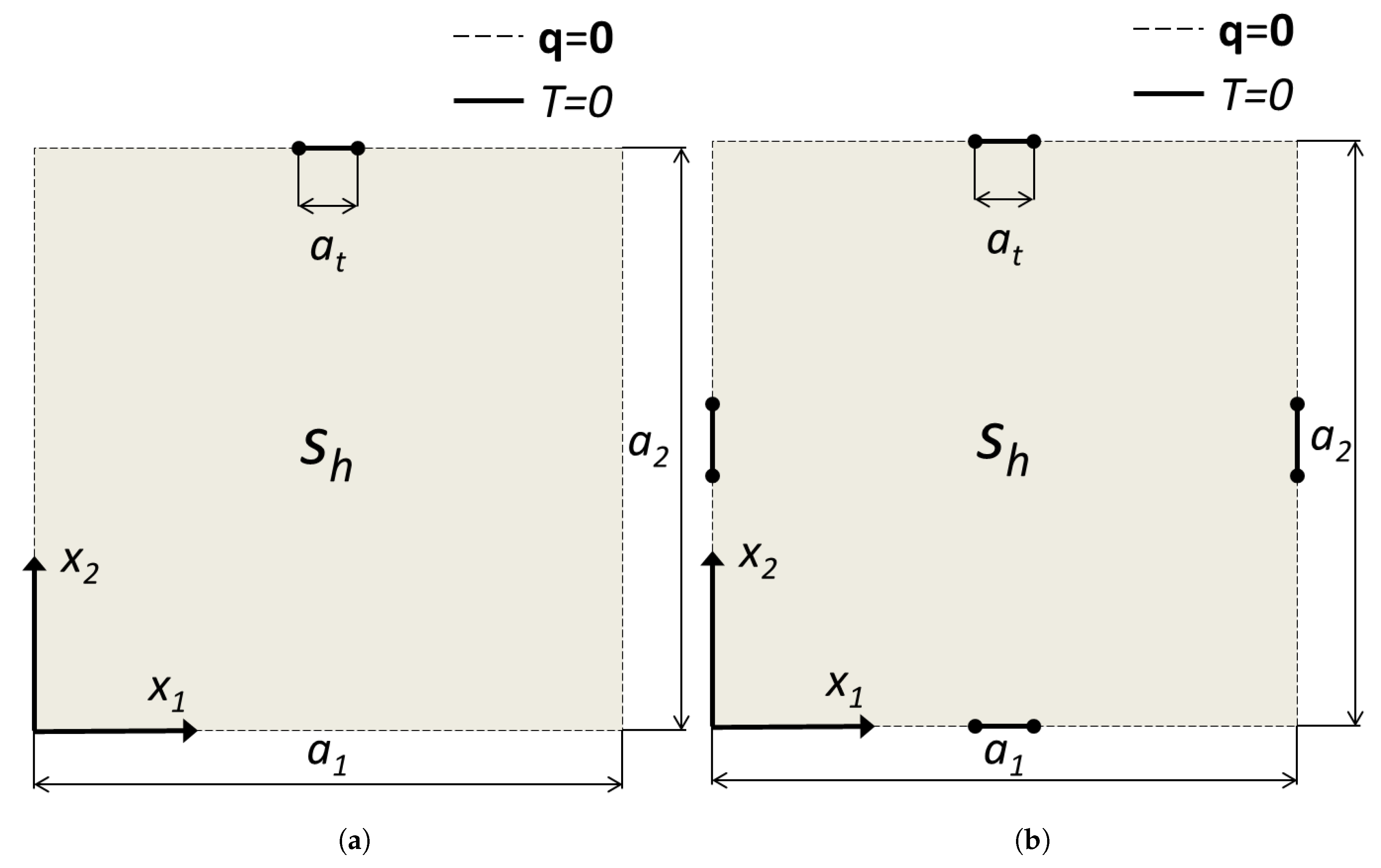
Two 2D benchmark problems are considered here: for each problem, the reference volume , appearing in the CNLPP formulation of Equation (19), is the overall area of the domain where the structure is embedded. The geometrical parameters and the BCs of each test case are illustrated in Figure 1. Benchmark 1 (BK1-2D), which has been taken from [43], is a plate having the following dimensions: m, m. A heating source Wm−2 is evenly distributed over the whole design domain. As far as BCs are concerned, the temperature is set to zero for nodes located at with m, while, on the rest of the boundary the adiabatic wall condition () is imposed. The FE model is made of PLANE55 elements (4 nodes with a single DOF per node).
The second benchmark problem (BK2-2D) is characterized by the same geometrical and material properties of BK1-2D, the only difference being in the applied BCs. In this case, a zero temperature is applied on four heat skins located at and , with , whilst a heat flux is set on the other regions of the boundary. In addition, in this case, the mesh of the FE model is made of PLANE55 elements.
For both test cases, the reference volume is and the volume fraction appearing in Equation (19) has been set as . An initial guess characterized by a uniform pseudo-density field has been considered for each analysis. The reference thermal compliance appearing in Equation (19) corresponds to the thermal compliance of the initial guess: its value is 5.956 WK for BK1-2D and 1.0389 WK for BK2-2D.
4.1.1. BK1-2D: Sensitivity of the Optimized Topology to the B-Spline and NURBS Entities Integer Parameters
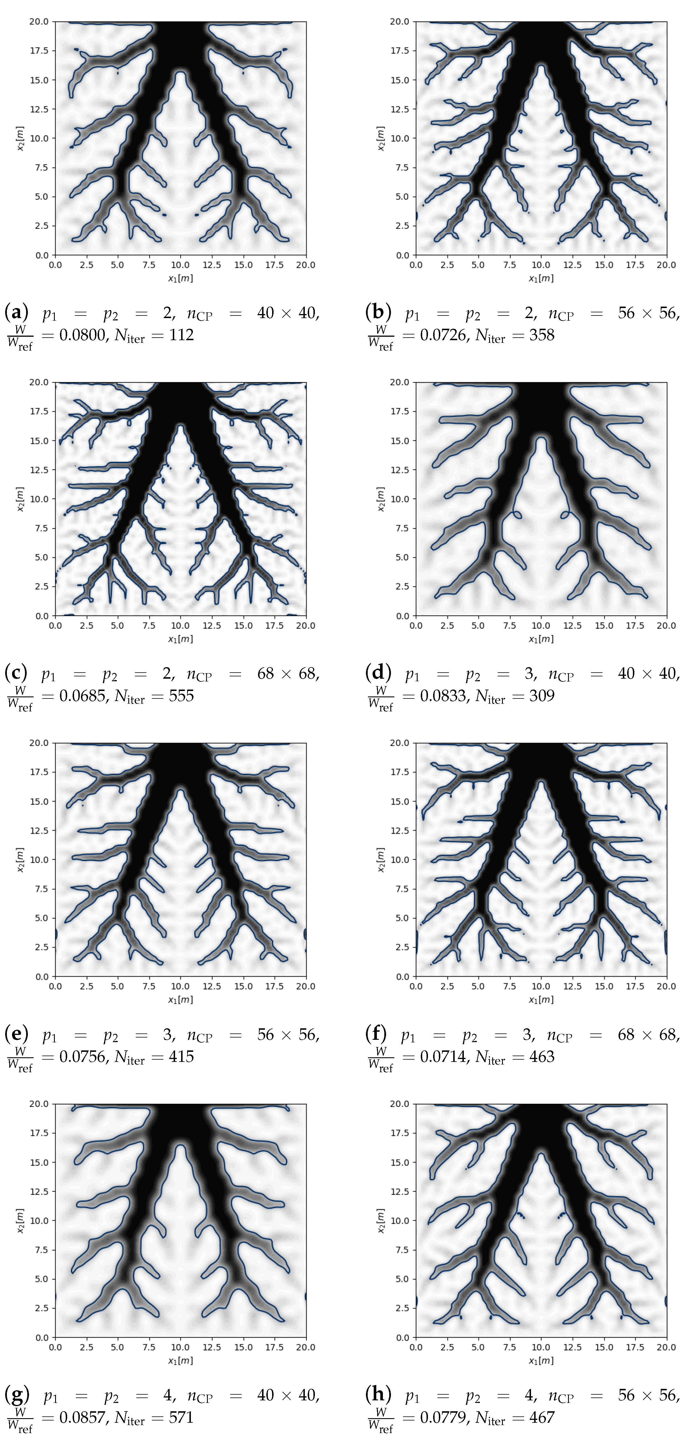
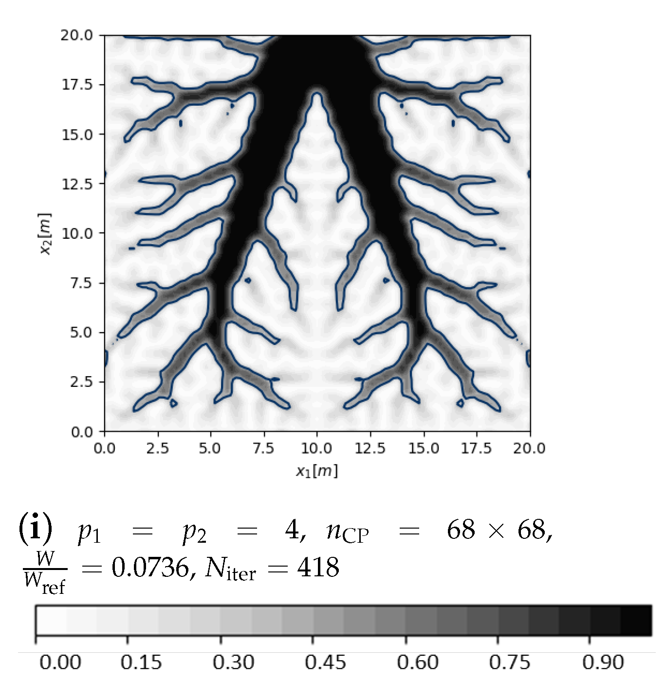
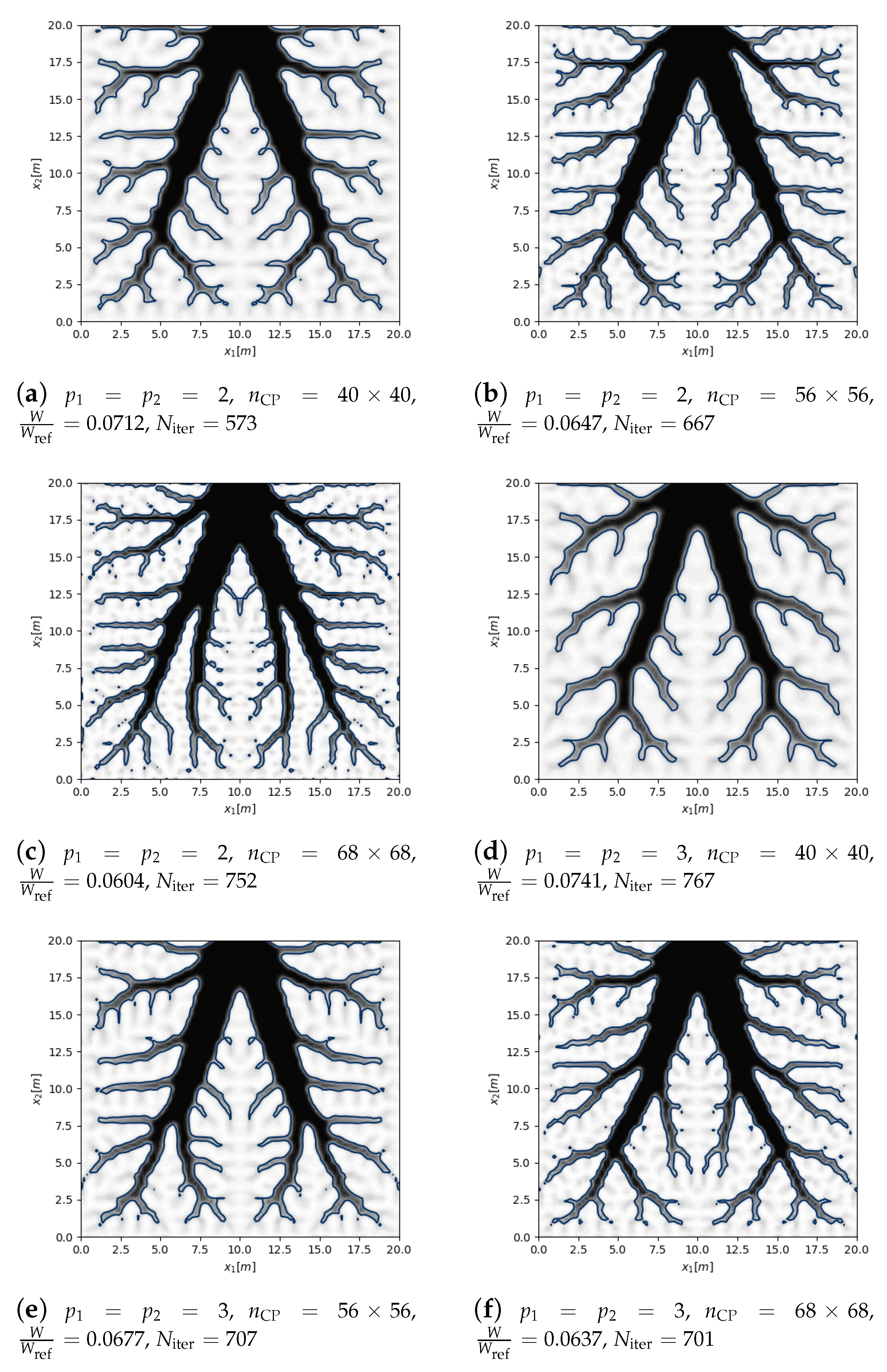
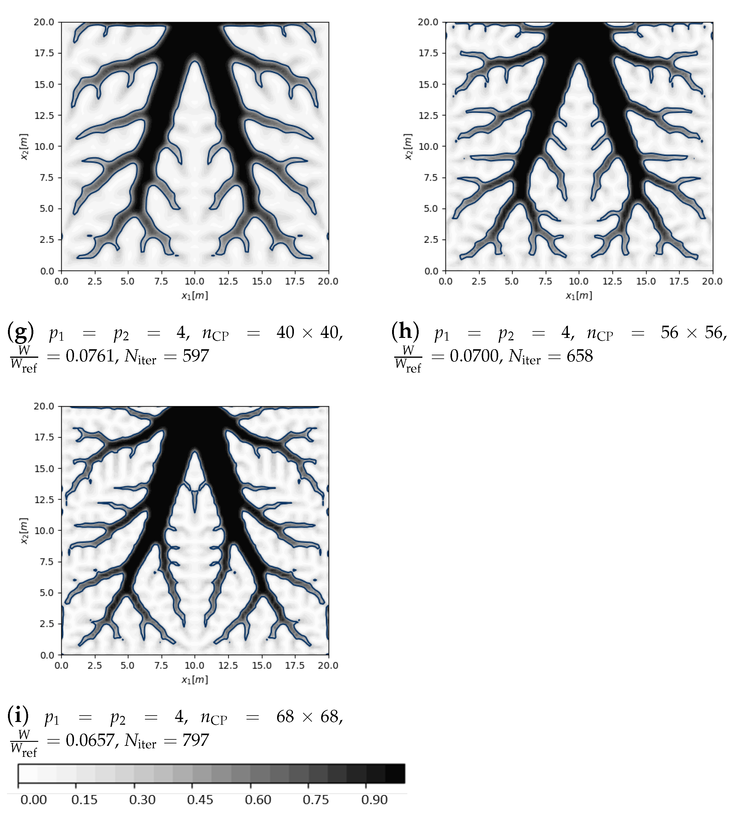
An extensive numerical campaign of tests has been performed on BK1-2D: the aim is to study the sensitivity of the optimized topology to the integer parameters involved in the definition of B-spline and NURBS entities. In particular, the CNLPP of Equation (19) is solved by considering the following combinations of blending functions degrees and CPs numbers: (a) , (); (b) for both B-spline and NURBS entities. Moreover, in this case, the CNLPP formulation has been enhanced by adding a symmetry constraint with respect to plane .
Results are provided in terms of dimensionless thermal compliance and number of iterations to achieve convergence for B-spline and NURBS entities in Figure 2 and Figure 3, respectively. For each solution, the requirement on the volume fraction is always satisfied.
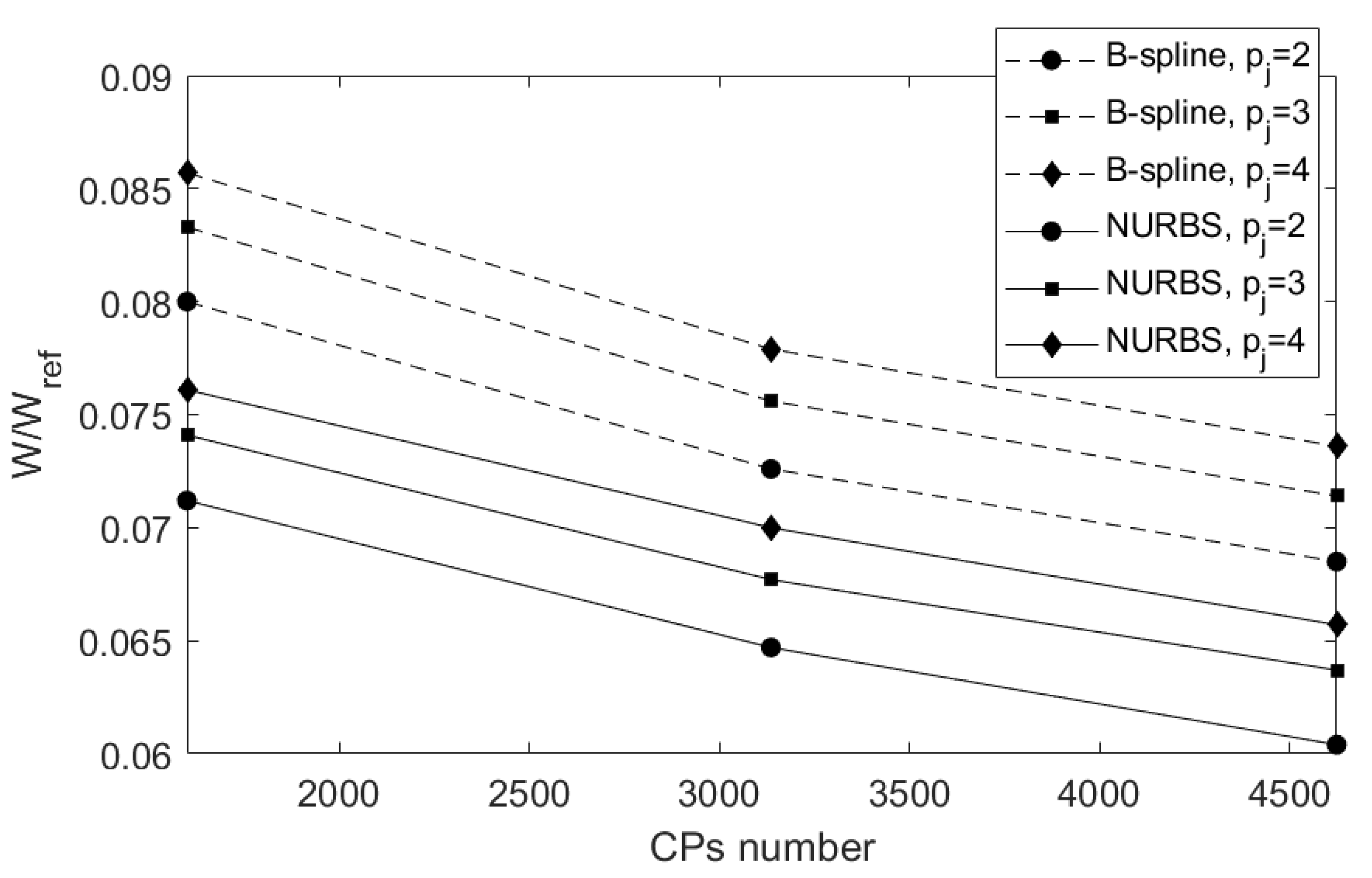
A synthesis of the results illustrated in Figure 2 and Figure 3 is shown in Figure 4, where the dimensionless thermal compliance is plotted versus the number of CPs and blending functions degrees. Some remarks can be inferred from the analysis of these results.
- For B-spline and NURBS solutions, the higher the number of CPs (or the lower the degree) the smaller the objective function value. As explained in [32,33], this is due to the local support size: the higher the CPs number for a given degree (or the lower the degree for a given number of CPs) the smaller the local support size, consequently smaller topological branches appear in optimized topologies. Moreover, the higher the degree (for a given CPs number) the smoother the boundary of the final topology.
- The NURBS local support can be associated to the concept of the filter zone in standard density-based TO algorithms, as stated in Section 3. According to the definition of the local support of Equation (9), the higher the degree (or the smaller the CPs number) the wider the local support; thus, a single control point affects a wider region of the computation domain. Indeed, as discussed in [35], the local support of Equation (9) enforces a minimum length scale in the optimized topology. Consequently, it can be stated that a high number of CPs and small degrees should be considered if minimum member size does not constitute a restriction for the problem at hand. High degrees and/or small CPs number should be considered otherwise.
- The effect of including the weights among the design variables is twofold: on the one hand, weights contribute to improve the final performances (the objective function of a NURBS solution is always lower than the one of a B-spline solution), whilst, on the other hand, they allow for obtaining optimized topologies characterized by a boundary smoother than the B-spline counterpart.
- The constraint on the volume fraction gets a very small negative value (between and 0) for the optimized topologies resulting from problem (19); thus, the local minimizer is located on the boundary between feasible and infeasible regions.
- All the analyses were performed on a work-station with an Intel Xeon E5-2697v2 processor (2.70–3.50 GHz, Santa Clara, CA, USA) and four cores dedicated to the optimization calculations. The highest computational time occurs for the NURBS solution illustrated in Figure 3 (i), which required about 1.5 h to find the local feasible minimizer.
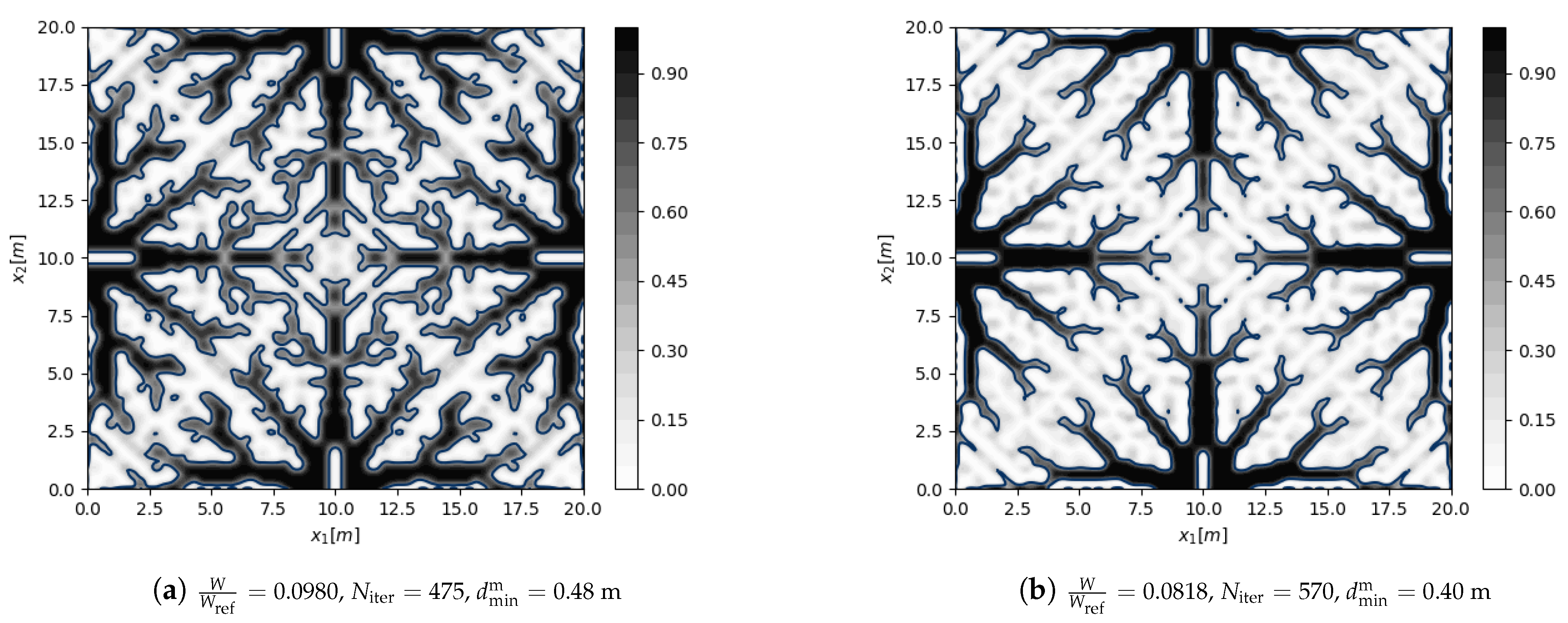
4.1.2. BK2-2D: Minimum Member Size Effect on the Optimized Topology
The influence of the minimum member size requirement is investigated on BK2-2D. In particular, the CNLPP formulation of Equation (19) has been enhanced by considering a constraint on the minimum length scale requirement: the minimum dimension of the optimized topology should be greater than or equal to m. To automatically satisfy the minimum length scale requirement without introducing an explicit constraint in the problem formulation, according to the methodology presented in [35], B-spline and NURBS entities with and CPs are used for this analysis. Moreover, the topology is constrained to be symmetric with respect to planes and .
The optimized topologies solution of problem (19) are shown in Figure 5, for both B-spline and NURBS entities: numerical results are provided in terms of dimensionless thermal compliance , number of iterations to achieve convergence and measured minimum member size , i.e., the minimum length scale measured after CAD reconstruction of the boundary of the optimized topology [35]. For each solution, the requirement on the volume fraction is always satisfied (this constraint is always almost active, in the sense that it takes a very small negative value between and 0).
As expected, the NURBS solution is characterized by a dimensionless thermal compliance lower than the B-spline counterpart. Moreover, thanks to the geometrical properties of the NURBS blending functions, the requirement on the minimum length scale is always satisfied. In particular, it is noteworthy that the minimum length scale constraint is almost active for the NURBS solution illustrated in Figure 5.
4.2. A 3D Benchmark Problem
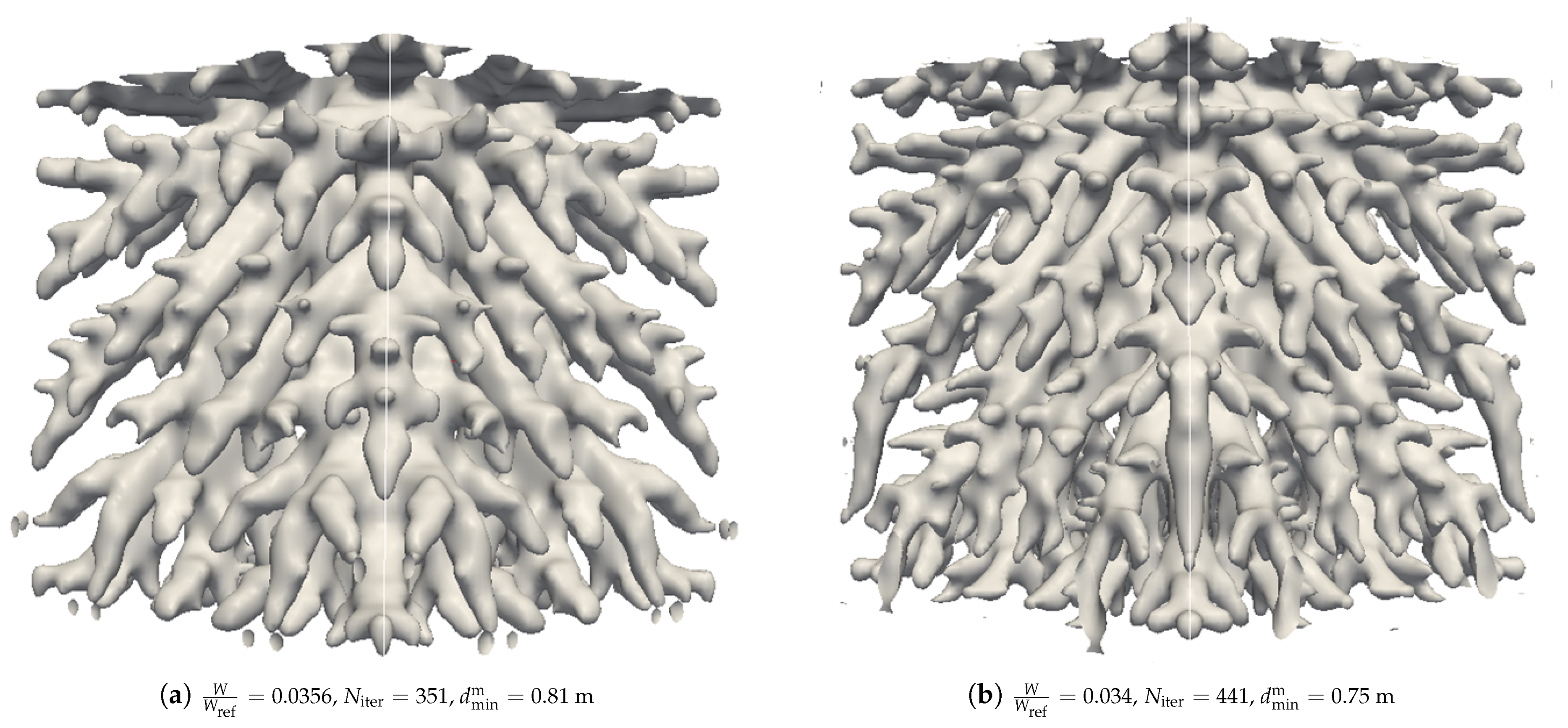
The third benchmark (BK1-3D) deals with the TO of the 3D cubic domain illustrated in Figure 6; the geometry of BK1-3D is characterized by the following dimensions: m, m. The material properties are the same as those used in test cases BK1-2D and BK2-2D.
The FE model is made of SOLID279 elements (eight nodes, one DOF per node). A null temperature is imposed on the nodes belonging to the heat skin located at , while a zero heat flux is imposed on the rest of the boundary. A heating source Wm−3 is evenly distributed over the whole design domain.
Regarding problem (19), the reference volume and the volume fraction are and , respectively. An initial guess characterized by a uniform pseudo-density field is considered. The reference thermal compliance associated to the starting point is WK. Furthermore, three design requirements have been added to the CNLPP formulation of Equation (19): a minimum member size requirement m and a double orthogonal symmetry constraint with respect to planes and . According to the methodology described in [35], the minimum length scale requirement is fulfilled by choosing a B-spline/NURBS entity characterized by , () and .
The optimized topologies are illustrated in Figure 7, for both B-spline and NURBS entities: numerical results are provided in terms of dimensionless thermal compliance , number of iterations and measured minimum member size . For each solution, the requirement on the volume fraction is active. The same remarks already done for benchmark problem BK2-2D can be repeated here.
5. Conclusions
In this work, steady-state thermal conduction TO problems have been revisited in the context of a special SIMP approach reformulated in the framework of the NURBS hyper-surfaces theory. Some features of this approach have to be highlighted.
- NURBS hyper-surfaces bring three advantages: (a) unlike the classical SIMP approach, a filter zone does not need to be introduced because the NURBS local support establishes an implicit relationship among the pseudo-density of contiguous mesh elements; (b) when compared to the classical SIMP approach, the number of design variables is reduced; (c) the CAD reconstruction of the boundary of the optimized topology is an easy task.
- A sensitivity analysis of the optimized topology to the NURBS integer parameters has been performed. Some general rules about the choice of the integer parameters can be drawn: the higher the number of CPs (for a given degree) or the lower the degree (for a given number of CPs) the smaller the objective function value, for both B-spline and NURBS solutions.
- The role of NURBS weights has been evaluated. In particular, by keeping the same number of CPs and the same degrees, the objective function of the NURBS solution is lower than that of the B-spline counterpart.
- The minimum-length scale requirement is correctly taken into account, without introducing an explicit optimization constraint, by properly setting the integer parameters of the NURBS entity. This is one of the most important advantages of the NURBS-based SIMP approach.
- The topological descriptor is not related to the mesh of the FE model. The FE model is only used to assess the physical responses of the problem at hand. The optimized topology can be easily extracted at the end of the optimization process because it is described by means of a pure geometrical entity, i.e., a CAD-compatible entity.
Relevant paths to take for future works include: (i) the integration of the transient regime within the TO problem formulation; (ii) the implementation of thermo-mechanics problems (by considering both weak and strong couplings); (iii) the extension of the proposed approach to design-dependent boundary conditions in order to deal with more realistic engineering applications. Research is ongoing on all the above aspects.
Author Contributions
M.M.: conceptualization, methodology, software, validation, formal analysis, investigation, resources, writing—original draft preparation, writing—review and editing, supervision, funding acquisition. K.R.: investigation, writing—original draft preparation. All authors have read and agreed to the published version of the manuscript.
Funding
This work has been funded by Nouvelle-Aquitaine region through OCEAN-ALM project.
Data Availability Statement
The raw/processed data required to reproduce these findings cannot be shared at this time as the data also forms part of an ongoing study.
Conflicts of Interest
The authors declare no conflict of interest.
References
- Garimella, V.; Fleischer, A.; Murthy, J.; Keshavarzi, A.; Prasher, R.; Patel, C.; Bhavnani, S.; Venkatasubramanian, R.; Mahajan, R.; Joshi, Y.; et al. Thermal Challenges in Next-Generation Electronic Systems. IEEE Trans. Compon. Packag. Technol. 2008, 31, 2577–2592. [Google Scholar] [CrossRef]
- Vassighi, A.; Sachdev, M. Thermal and Power Management of Integrated Circuits; Springer Science & Business Media: New York, NY, USA, 2006. [Google Scholar]
- Dong, X.; Liu, X. Multi-objective optimal design of microchannel cooling heat sink using topology optimization method. Numer. Heat Transf. Part A Appl. 2020, 77, 90–104. [Google Scholar] [CrossRef]
- Zhao, M.; Tian, Y.; Hu, M.; Zhang, F.; Yang, M. Topology optimization of fins for energy storage tank with phase change material. Numer. Heat Transf. Part A Appl. 2020, 77, 284–301. [Google Scholar] [CrossRef]
- Wang, S.; Li, S.; Luo, L.; Zhao, Z.; Du, W.; Sundén, B. A high temperature turbine blade heat transfer multilevel design platform. Numer. Heat Transf. Part A Appl. 2021, 79, 122–145. [Google Scholar] [CrossRef]
- Sun, S.; Liebersbach, P.; Qian, X. 3D topology optimization of heat sinks for liquid cooling. Appl. Therm. Eng. 2020, 178, 115540. [Google Scholar] [CrossRef]
- Zhang, B.; Zhu, J.; Gao, L. Topology optimization design of nanofluid-cooled microchannel heat sink with temperature-dependent fluid properties. Appl. Therm. Eng. 2020, 176, 115354. [Google Scholar] [CrossRef]
- Malekipour, E.; Tovar, A.; El-Mounayri, H. Heat Conduction and Geometry Topology Optimization of Support Structure in Laser-Based Additive Manufacturing. Mech. Addit. Adv. Manuf. 2018, 9, 17–27. [Google Scholar]
- Bendsoe, M.; Kikuchi, N. Generating optimal topologies in structural design using a homogenization method. Comput. Methods Appl. Mech. Eng. 1988, 71, 197–224. [Google Scholar] [CrossRef]
- Bendsoe, M.; Sigmund, O. Topology Optimization-Theory, Methods and Applications; Springer: Berlin/Heidelberg, Germany, 2003. [Google Scholar]
- Eschenauer, H.; Olhoff, N. Topology Optimization of Continuum Structures: A Review. Appl. Mech. Rev. 2001, 54, 331–389. [Google Scholar] [CrossRef]
- Suzuki, K.; Kikuchi, N. A homogenization method for shape and topology optimization. Comput. Methods Appl. Mech. Eng. 2001, 93, 291–318. [Google Scholar] [CrossRef] [Green Version]
- Bendsoe, M. Optimal shape design as a material distribution problem. Struct. Optim. 1989, 1, 193–202. [Google Scholar] [CrossRef]
- Sethian, J.; Wiegmann, A. Structural Boundary Design via Level Set and Immersed Interface Methods. J. Comput. Phys. 2000, 163, 489–528. [Google Scholar] [CrossRef]
- Wang, M.; Wang, X.; Guo, D. A level set method for structural topology optimization. Comput. Methods Appl. Mech. Eng. 2013, 192, 227–246. [Google Scholar] [CrossRef]
- Guo, X.; Zhang, W.; Zhang, J.; Yuan, J. Explicit structural topology optimization based on moving morphable components (MMC) with curved skeletons. Comput. Methods Appl. Mech. Eng. 2016, 310, 711–748. [Google Scholar] [CrossRef]
- Xie, Y.M.; Steven, G.P. A simple evolutionary procedure for structural optimization. Comput. Struct. 1993, 49, 885–896. [Google Scholar] [CrossRef]
- Huang, X.; Xie, Y.M. Bi-directional evolutionary topology optimization of continuum structures with one or multiple materials. Comput. Mech. 2009, 43, 393. [Google Scholar] [CrossRef]
- Huang, X.; Xie, Y.M. Evolutionary Topology Optimization of Continuum Structures: Methods and Applications; John Wiley & Sons, Ltd: Hoboken, NJ, USA, 2010. [Google Scholar]
- Li, Q.; Steven, G.P.; Querin, O.M.; Xie, Y.M. Shape and topology design for heat conduction by evolutionary structural optimization. Int. J. Heat Mass Transf. 1999, 42, 3361–3371. [Google Scholar] [CrossRef]
- Li, Q.; Steven, G.P.; Xie, Y.M.; Querin, O.M. Evolutionary topology optimization for temperature reduction of heat conducting fields. Int. J. Heat Mass Transf. 2004, 47, 5071–5083. [Google Scholar] [CrossRef]
- Zhuang, C.G.; Xiong, Z.H.; Han, D. A level set method for topology optimization of heat conduction problem under multiple load cases. Comput. Method Appl. Mech. Eng. 2007, 196, 1074–1084. [Google Scholar] [CrossRef]
- Yoon, G. Topological design of heat dissipating structure with forced convective heat transfer. J. Mech. Sci. Technol. 2010, 24, 1225–1233. [Google Scholar] [CrossRef]
- Ikonen, T.; Marck, G.; Sóbester, A.; Keane, A. Topology optimization of conductive heat transfer problems using parametric L-systems. Struct. Multidiscip. Optim. 2018, 58, 1899–1916. [Google Scholar] [CrossRef] [Green Version]
- Hu, D.; Zhang, Z.; Li, Q. Numerical study on flow and heat transfer characteristics of microchannel designed using topological optimizations method. Sci. China Tech. Sci. 2020, 63, 105–115. [Google Scholar] [CrossRef]
- Yoon, M.; Koo, B. Topology design optimization of conductive thermal problems subject to design-dependent load using density gradients. Adv. Mech. Eng. 2019, 11, 1–11. [Google Scholar] [CrossRef]
- Iga, A.; Nishiwaki, S.; Izui, K.; Yoshimura, M. Topology optimization for thermal conductors considering design-dependent effects, including heat conduction and convection. Int. J. Heat Mass Transf. 2009, 52, 2721–2732. [Google Scholar] [CrossRef]
- Dbouk, T. A review about the engineering design of optimal heat transfer systems using topology optimization. Appl. Therm. Eng. 2017, 112, 841–854. [Google Scholar] [CrossRef]
- Allaire, G. Shape Optimization by the Homogenization Method; Springer: New York, NY, USA, 2002. [Google Scholar]
- Guest, J.K.; Prévost, J.H.; Belytschko, T. Achieving minimum length scale in topology optimization using nodal design variables and projection functions. Int. J. Numer. Methods Eng. 2003, 61, 238–254. [Google Scholar] [CrossRef]
- Lazarov, B.S.; Wang, F.; Sigmund, O. Length scale and manufacturability in density-based topology optimization. Arch. Appl. Mech. 2016, 86, 189–218. [Google Scholar] [CrossRef] [Green Version]
- Costa, G.; Montemurro, M.; Pailhès, J. A 2D topology optimisation algorithm in NURBS framework with geometric constraints. Int. J. Mech. Mater. Des. 2018, 14, 669–696. [Google Scholar] [CrossRef] [Green Version]
- Costa, G.; Montemurro, M.; Pailhès, J. NURBS Hyper-surfaces for 3D Topology Optimisation Problems. Mech. Adv. Mater. Struct. 2021, 28, 665–684. [Google Scholar] [CrossRef]
- Costa, G.; Montemurro, M.; Pailhès, J.; Perry, N. Maximum length scale requirement in a topology optimisation method based on NURBS hyper-surfaces. CIRP Ann. 2019, 68, 153–156. [Google Scholar] [CrossRef] [Green Version]
- Costa, G.; Montemurro, M.; Pailhès, J. Minimum Length Scale Control in a NURBS-based SIMP Method. Comput. Methods Appl. Mech. Eng. 2019, 354, 963–989. [Google Scholar] [CrossRef]
- Rodriguez, T.; Montemurro, M.; Le Texier, P.; Pailhès, J. Structural Displacement Requirement in a Topology Optimization Algorithm Based on Isogeometric Entities. J. Optim. Theory Appl. 2020, 184, 250–276. [Google Scholar] [CrossRef]
- Bertolino, G.; Montemurro, M.; Perry, N.; Pourroy, F. An Efficient Hybrid Optimization Strategy for Surface Reconstruction. Computer Graphics Forum 2021. [Google Scholar] [CrossRef]
- Costa, G.; Montemurro, M. Eigen-frequencies and harmonic responses in topology optimisation: A CAD-compatible algorithm. Eng. Struct. 2020, 214, 110602. [Google Scholar] [CrossRef]
- Montemurro, M.; Bertolino, G.; Roiné, T. A General Multi-Scale Topology Optimisation Method for Lightweight Lattice Structures Obtained through Additive Manufacturing Technology. Compos. Struct. 2021, 258, 113360. [Google Scholar] [CrossRef]
- Piegl, L.; Tiller, W. The NURBS Book; Springer: Berlin/Heidelberg, Germany; New York, NY, USA,, 1997. [Google Scholar]
- Zienkiewicz, O.C.; Taylor, R.L.; Zhu, J.Z. The Finite Element Method: Its Basis and Fundamentals; Elsevier: Amsterdam, The Netherlands, 2005. [Google Scholar]
- Svanberg, K. A class of globally convergent optimization methods based on conservative convex separable approximations. SIAM J. Optim. 2002, 12, 555–573. [Google Scholar] [CrossRef] [Green Version]
- Alexandersen, J. Topology Optimization for Convection Problems. Master’s Thesis, DTU Mekanik, Kongens Lyngby, Denmark, 2011. [Google Scholar]
Figure 1.
Geometry and boundary conditions of benchmark problems (a) BK1-2D and (b) BK2-2D.

Figure 2.
Benchmark problem BK1-2D: sensitivity of the optimized topology to CP number and basis functions degrees, B-spline solutions of problem (19); the grey-scale bar refers to the pseudo-density field of Equation (16).


Figure 3.
Benchmark problem BK1-2D: sensitivity of the optimized topology to CP number and basis functions degrees, NURBS solutions of problem (19); the grey-scale bar refers to the pseudo-density field of Equation (16).


Figure 4.
Benchmark problem BK1-2D: dimensionless thermal compliance versus CPs number and degrees for B-spline and NURBS solutions
Figure 4.
Benchmark problem BK1-2D: dimensionless thermal compliance versus CPs number and degrees for B-spline and NURBS solutions

Figure 5.
Benchmark problem BK2-2D: (a) B-spline and (b) NURBS solutions of problem (19) with and ; the grey-scale bar refers to the pseudo-density field of Equation (16).

Figure 6.
Geometry and boundary conditions of benchmark problem BK1-3D.

Figure 7.
Benchmark problem BK1-3D: (a) B-spline and (b) NURBS solutions of problem (19) with and .
Figure 7.
Benchmark problem BK1-3D: (a) B-spline and (b) NURBS solutions of problem (19) with and .


Table 1.
GC-MMA algorithm parameters.
| Parameter | Value |
|---|---|
| move | 0.1 |
| albefa | 0.1 |
| Stop Criterion | Value |
| Maximum n. of function evaluations | |
| Maximum n. of iterations | 1000 |
| Tolerance on objective function | |
| Tolerance on constraints | |
| Tolerance on input variables change | |
| Tolerance on Karush–Kuhn–Tucker norm |
Publisher’s Note: MDPI stays neutral with regard to jurisdictional claims in published maps and institutional affiliations. |
© 2021 by the authors. Licensee MDPI, Basel, Switzerland. This article is an open access article distributed under the terms and conditions of the Creative Commons Attribution (CC BY) license (https://creativecommons.org/licenses/by/4.0/).
Share and Cite
MDPI and ACS Style
Montemurro, M.; Refai, K. A Topology Optimization Method Based on Non-Uniform Rational Basis Spline Hyper-Surfaces for Heat Conduction Problems. Symmetry 2021, 13, 888. https://0-doi-org.brum.beds.ac.uk/10.3390/sym13050888
AMA Style
Montemurro M, Refai K. A Topology Optimization Method Based on Non-Uniform Rational Basis Spline Hyper-Surfaces for Heat Conduction Problems. Symmetry. 2021; 13(5):888. https://0-doi-org.brum.beds.ac.uk/10.3390/sym13050888
Chicago/Turabian StyleMontemurro, Marco, and Khalil Refai. 2021. "A Topology Optimization Method Based on Non-Uniform Rational Basis Spline Hyper-Surfaces for Heat Conduction Problems" Symmetry 13, no. 5: 888. https://0-doi-org.brum.beds.ac.uk/10.3390/sym13050888
Note that from the first issue of 2016, this journal uses article numbers instead of page numbers. See further details here.