An Unsupervised Learning Method for Attributed Network Based on Non-Euclidean Geometry

Abstract

Many real-world networks can be modeled as attributed networks, where nodes are affiliated with attributes. When we implement attributed network embedding, we need to face two types of heterogeneous information, namely, structural information and attribute information. The structural information of undirected networks is usually expressed as a symmetric adjacency matrix. Network embedding learning is to utilize the above information to learn the vector representations of nodes in the network. How to integrate these two types of heterogeneous information to improve the performance of network embedding is a challenge. Most of the current approaches embed the networks in Euclidean spaces, but the networks themselves are non-Euclidean. As a consequence, the geometric differences between the embedded space and the underlying space of the network will affect the performance of the network embedding. According to the non-Euclidean geometry of networks, this paper proposes an attributed network embedding framework based on hyperbolic geometry and the Ricci curvature, namely, RHAE. Our method consists of two modules: (1) the first module is an autoencoder module in which each layer is provided with a network information aggregation layer based on the Ricci curvature and an embedding layer based on hyperbolic geometry; (2) the second module is a skip-gram module in which the random walk is based on the Ricci curvature. These two modules are based on non-Euclidean geometry, but they fuse the topology information and attribute information in the network from different angles. Experimental results on some benchmark datasets show that our approach outperforms the baselines.

1. Introduction

Networks are used to model and analyze complex systems, such as social networks, biological compounds, and citation networks. The complex structure of networks presents a great challenge to tasks involving network embedding. As a new approach, network embedding [1,2], which maps network nodes to low-dimensional vector representations, can deal with this problem well. The obtained node representations can be further applied to node classification [3], graph classification [4,5], recommendation [6,7], community detection [8,9], etc. Take the Cora dataset used in the experimental part of this paper as an example. The dataset contains 2708 papers with 5278 citation relationships between them. We think of papers as nodes and reference relationships as edges, and we obtain the network topology. The vocabulary of the dataset is composed of 1433 words, so the word vector corresponding to each paper is constructed as follows: the dimension of the word vector is 1433; each element of the word vector corresponds to a word, and this element only has two possible values of 0 or 1; a value of 0 means that the word corresponding to the element is not in the paper, and a value of 1 means that it is in the paper. The resulting word vector is the attribute of the node. All papers are divided into seven categories, which are: neural networks, rule learning, reinforcement learning, probabilistic methods, theory, genetic algorithms, case-based. These seven categories are then converted into seven numbers that serve as node labels. The adjacency matrix and node attributes are input into the neural network model to obtain network embedding, which then are classified by a simple classifier. By comparing the classification results with the node labels on a computer, we can know the accuracy of the classification.

The starting point of network embedding is to keep some information of the network, such as proximity, during the embedding process. Many network embedding methods [10,11] use the topological information of the network to learn the vector representations of nodes, meaning that the target node and its first-order or higher-order neighbors are close to each other in the embedding space, while the node pairs without neighbor relations are far away from each other. Adjacent relations can be determined by an adjacency matrix and its power [12], and they can also be determined by random walk sampling [13]. However, in many real networks, nodes are often associated with rich attribute features. If only structural information is considered in the process of learning attributed network embedding, the results are often not satisfactory. Therefore, in the existing works, researchers fused network structural information and attribute information in various ways to improve the performance of network embedding. Some methods [14], in essence, separate the processing of structural information and attribute information in the process of learning embeddings and then obtain the embeddings of attribute networks by establishing the correlation between structural information and attribute information. Other methods [15,16] first build a new network according to the similarity between node attributes, which forms a heterogeneous network with the original network, and then integrate the learning of the two networks through random walks. However, the correlations in such methods are more artificially added and may be inconsistent with the correlations contained in the structural data and attribute data themselves; that is to say, the correlations between the actual structural information and attribute information are artificially exaggerated or reduced. Structural data and attribute data are two types of heterogeneous information sources. It is usually difficult to judge the correlation between them manually; therefore, the correlation mined through the data structure itself can be better in line with the reality. The methods mentioned above are all based on Euclidean geometry, and some recent works [17,18,19] have begun to explore how to use hyperbolic geometry to improve the performance of network embedding. Hyperbolic geometry has shown its advantages in the embedding representation of hierarchical data, but thus far, the tools used in these applications are limited to hyperbolic geometry and do not incorporate other tools in non-Euclidean geometry, such as the Ricci curvature.

Based on previous analysis, this paper proposes a new framework based on non-Euclidean geometry to learn the embeddings of attributed networks and considers the following questions: (1) How can the structural information and attribute information of the attributed network be effectively integrated? (2) How can the neighborhood be effectively defined, and how can the strength of the neighborhood relationship between the target node and its neighbors be defined? (3) How can hyperbolic geometry or, more generally, non-Euclidean geometry be effectively integrated into our framework to improve model performance? Inspired by ANRL [20], our model combines the autoencoder module with the random walk module, but our model is fundamentally different from the ANRL model, which will be discussed in detail in the following analysis. The main contributions of our paper are as follows: (1) The random walk module in our model guides the random walk according to the Ricci curvature, in order to better distinguish the strength of the relationship between nodes, better explore the neighborhood of the target node, and obtain the generalized adjacent node pairs required for network embedding. (2) Our model, RHAE, combines the Ricci curvature and hyperbolic geometry to transform the embedded layers of the autocoder module to aggregate the structural information and attribute information of the attributed network more effectively. (3) On the benchmark datasets, we conduct extensive experiments to compare RHAE to the baseline approaches.

The rest of this article is organized as follows: Section 2 briefly reviews some related works on hyperbolic geometry, the Ricci curvature, and network embedding. Section 3 discusses the architecture of our model, RHAE, in detail. Section 4 presents the experimental results and provides a detailed analysis of the performance. Finally, Section 5 summarizes the paper and describes future work.

2. Related Work

In this section, we review some of the concepts in non-Euclidean geometry that we use later. We first introduce the basic models of hyperbolic geometry and some key concepts relevant to our work and then introduce the concepts of curvature in non-Euclidean geometry that are applicable to discrete objects such as networks. Finally, we discuss some related works.

2.1. Hyperbolic Geometry

The spaces usually used for data processing are Euclidean spaces, whose curvature is 0; that is to say, the Euclidean spaces are locally and globally flat. Euclidean spaces are a type of space of constant curvature. The spaces of constant curvature can be divided into three categories: Euclidean spaces, spherical spaces, and hyperbolic spaces. The curvatures of the last two types of spaces are, respectively, constant positive and constant negative. An important characteristic of hyperbolic spaces is that they expand exponentially, whereas Euclidean spaces can only expand at a polynomial rate [21]. In other words, the hyperbolic spaces are larger than the Euclidean spaces, which allows infinite trees to be embedded almost isometrically into the hyperbolic spaces. This characteristic of hyperbolic spaces makes them have advantages in expressing hierarchical data. However, because of the size difference of the spaces, it is difficult to embed the hyperbolic spaces into the Euclidean spaces without distortion. As a result, many models have been built to model hyperbolic spaces, but these models can only reflect some characteristics of hyperbolic spaces, and the hyperboloid model is one of them.

• Hyperboloid model. We first define the Minkowski space and the Minkowski product. The (n+1)-dimensional Minkowski space $R^{n+1}$ is a vector space endowed with the Minkowski inner product of the following form:

$$<u,v{>}_M=-u_0{v}_0+\sum _{i=1}^n{u}_i{v}_i$$

(1)

for $u,v\in R^{n+1}$.

Definition 1

([19,22]). The hyperboloid model $H^n$ of hyperbolic space is an n-dimensional manifold endowed with a Minkowski inner product, i.e.,

$$H^n=\{u\in R^{n+1}:<u,u{>}_M=-1,u_0>0\}.$$

(2)

The tangent space of $H^n$ at point p is the set of points orthogonal to p with respect to the Minkowski inner product, which is a Euclidean space, i.e.,

$$T_p{H}^n=\{u\in R^{n+1}:<u,p{>}_M=0\}.$$

(3)

The distance in the hyperbolic space $H^n$ is defined as

$$d_M(p,q)=arccosh(-<p,q{>}_M),$$

(4)

for $p,q\in H^n$.

The norm of $u\in T_p{H}^n$ is defined as

$${\parallel u\parallel }_M=\sqrt{<u,u{>}_M}.$$

(5)

Remark 1.

For $u,v\in T_p{H}^n$, let $g_p(u,v)=<u,v{>}_M$; then, $H^n$ is a manifold equipped with a Riemannian metric $g_p$.

• Logarithmic and exponential maps.The hyperbolic space is a metric space, but not a vector space, and the tangent spaces are the local Euclidean spaces glued to the hyperbolic space. Therefore, in order to operate on vectors in the hyperbolic space, we must first map the corresponding points in the hyperbolic space to their tangent spaces, perform operations related to vectors in the Euclidean tangent spaces, and then map the resulting vector back to the hyperbolic space. It is worth noting that an exponential map can map points in a hyperbolic space to the corresponding tangent space, while a logarithmic map can map points in a tangent space back to the hyperbolic space, and in the hyperboloid model, both have simple closed forms.

Proposition 1

([19]). For $p,q\in H^n$ and $u\in T_p{H}^n$, the exponential map of the hyperboloid model is defined as

$$ex{p}_p\left(u\right)={cosh(\parallel u\parallel }_M{)p+sinh(\parallel u\parallel }_M)\frac{u}{{\parallel u\parallel }_M},$$

(6)

and the logarithmic map of this model is given by

$$lo{g}_p\left(q\right)=d_M(p,q)\frac{q+<p,q{>}_{M}p}{\parallel q+<p,q{>}_M{p\parallel }_M}.$$

(7)

• Parrallel Transport. If p and q are two points on the hyperboloid $H^n$, then the parallel transport of the vector u from the tangent space $T_p{H}^n$ at p to the tangent space $T_q{H}^n$ at q is defined as

$$P_{p\to q}\left(u\right)=u-\frac{<lo{g}_p\left(q\right),u>}{d_M{(p,q)}^2}(lo{g}_p\left(q\right)+lo{g}_q\left(p\right)).$$

(8)

• Projections. The projection operation here is to project the vector onto the hyperboloid manifold and the corresponding tangent space, which is useful for the optimization process. Let $p=(p_0,p_{1:n})\in R^{n+1}$; then, it can be projected on the hyperboloid space $H^n$ in the following way:

$$Pro{j}_{R^{n+1}\to H^n}\left(p\right)=(\sqrt{1+\parallel p_{1:n}{\parallel }_2^2},p_{1:n}).$$

(9)

where ${\parallel ·\parallel }_2$ is the Euclidean norm.

Analogously, a point $u\in R^{n+1}$ can be projected onto the tangent space $T_p{H}^n$ as follows:

$$Pro{j}_{R^{n+1}\to T_p{H}^n}\left(u\right)=u+<p,u{>}_{M}p.$$

(10)

• Hyperboloid linear transform. The usual linear transformation in the Euclidean space is multiplying the weight matrix by the embedding vector, and then adding the bias vector. However, the hyperbolic space itself is not a vector space, in which matrix multiplication cannot be carried out directly. As a consequence, we must map the points in the hyperbolic space to the tangent space at the origin by the logarithmic map, multiply by the weight matrix in the tangent space, and then pull the result back to the hyperbolic manifold by the exponential map, i.e.,

$$W\otimes p^H=ex{p}_o(W·lo{g}_o\left(p^H\right)),$$

(11)

where $p^H$ is a point in the hyperboloid manifold, W is the weight matrix, and the tangent space involved in the logarithmic map $lo{g}_o(·)$ and exponential map $ex{p}_o(·)$ is the tangent space at the origin. Let b be a Euclidean vector in the tangent space $T_o{H}^n$; then, the bias addition defined for the hyperboloid manifold is

$$p^H\oplus b=ex{p}_{p^H}\left(P_{o\to p^H}\left(b\right)\right),$$

(12)

where $P_{o\to p^H}$ is the parallel transport operator.

2.2. Ricci Curvature and Scalar Curvature

The Ricci curvature is a basic and important concept in Riemannian geometry, which was generalized by Ollivier to discrete objects such as networks [23]. Ollivier’s Ricci curvature is defined with the aid of the optimal transport distance.The probability measure at each node in the network is defined first, and then the Ricci curvature of the edge is defined by the optimal transport distance between the corresponding probability measures of the two nodes associated with the edge. Let us first define the probability measures at the nodes.

Definition 2

([24,25]). Let $G=(V,E)$ be an undirected network, where V is the set of nodes and E is the set of edges. Then, the probability measure of node u is defined as

$$m_u\left(v\right)=\left\{\begin{array}{cc}\frac{1}{d_u},\hfill & ifv\in \mathsf{\Gamma }\left(u\right)\hfill \\ 0,\hfill & otherwise,\hfill \end{array}\right.$$

(13)

where $d_u$ is the degree of node u and $\mathsf{\Gamma }\left(u\right)$ is the set of neighbors of u.

Having the probability measures at the nodes, we define the Wasserstein distance between the probability measures.

Definition 3

([25]). Let G be an undirected network, and $m_u,m_v$ be two probability measures. Then, the Wasserstein distance between two measures is defined as

$$W(m_u,m_v)=\underset{\zeta }{inf}\sum _{u^{\prime }\in \mathsf{\Gamma }\left(u\right)}\sum _{v^{\prime }\in \mathsf{\Gamma }\left(v\right)}d(u^{\prime },v^{\prime })\zeta (u^{\prime },v^{\prime }),$$

(14)

where $d(u,v)$ is the shortest path length between the nodes $u,v$, and ζ should satisfy the following conditions:

$$\sum _{u^{\prime }\in \mathsf{\Gamma }\left(u\right)}\zeta (u^{\prime },v^{\prime })=m_v\left(v^{\prime }\right),\sum _{v^{\prime }\in \mathsf{\Gamma }\left(v\right)}\zeta (u^{\prime },v^{\prime })=m_u\left(u^{\prime }\right).$$

(15)

Consequently, we can utilize the Wasserstein distance to define the Ricci curvature of the edges in the network.

Definition 4

([23,24]). Let $G=(V,E)$ be an undirected network; then, the Ricci curvature of edge $(u,v)$ is defined as

$$\kappa (u,v)=1-W(m_u,m_v),$$

(16)

where $u,v$ are the nodes of network G.

Next, we give the definition of the scalar curvatures of nodes.

Definition 5

([26]). Let $G=(V,E)$ be a network and $u\in V$ be a node of network G. Let $\mathsf{\Gamma }\left(u\right)$ be the set of neighbors of u. The scalar curvature of node u is

$$S_R\left(u\right)=\sum _{u^{\prime }\in \mathsf{\Gamma }\left(u\right)}\kappa (u,u^{\prime }).$$

(17)

2.3. Related Work

In recent years, in order to improve the performance of attributed network embedding, various methods have been adopted to integrate structural similarity and attribute similarity. DANE [27] uses two autoencoders to deal with the topological information and the attribute information and then establishes the correlation between the hidden layer representations of the two neural network models. With this correlation, it attempts to fuse the two heterogeneous information types and thus obtains the node representations. SNE [28] adopts the strategy of early fusion, which feeds the structural data and attribute data into the full connection layer to obtain the preliminary compressed representations, and then it inputs the two representations into the same multi-layer perceptron. Finally, it carries out training with the loss function that predicts the connection probability, in order to achieve the purpose of fusion of the heterogeneous data. The modeling scope of ANAE [29] has been expanded from a single node to a local subgraph. By modeling the local subgraph of the network, attribute information and structural information are fused to learn the node representations. FANE [16] maps attributes to virtual nodes in the network to build a new network, in order to unify the heterogeneity of the structure and attribute information sources, and defines a new random walk strategy to make use of attribute information to make the two types of information merge. ANRL [20] first models node attribute information through the autoencoder, but its reconstructed object is not the target node itself, but the neighbors of the target node. Then, the relationship between each node and its generalized neighbors is represented by the attribute-aware skip-gram model to capture the network structure.

3. Methods

3.1. Problem Setting

Let $G=(V,E,A,X)$ be an attributed network, where V denotes the set of nodes, E represents the set of edges, A represents the symmetric adjacency matrix of the network, and X is the matrix of the node attributes.

Definition 6.

Given an undirected and attributed network $G=(V,E,A,X)$, we aim to define a mapping function $f:u_i\to y_i\in R^d$ for every node $u_i\in V$, where $d<<\left|V\right|$ and f preverses both the structure proximity and attribute proximity.

3.2. Non-Euclidean Autoencoder

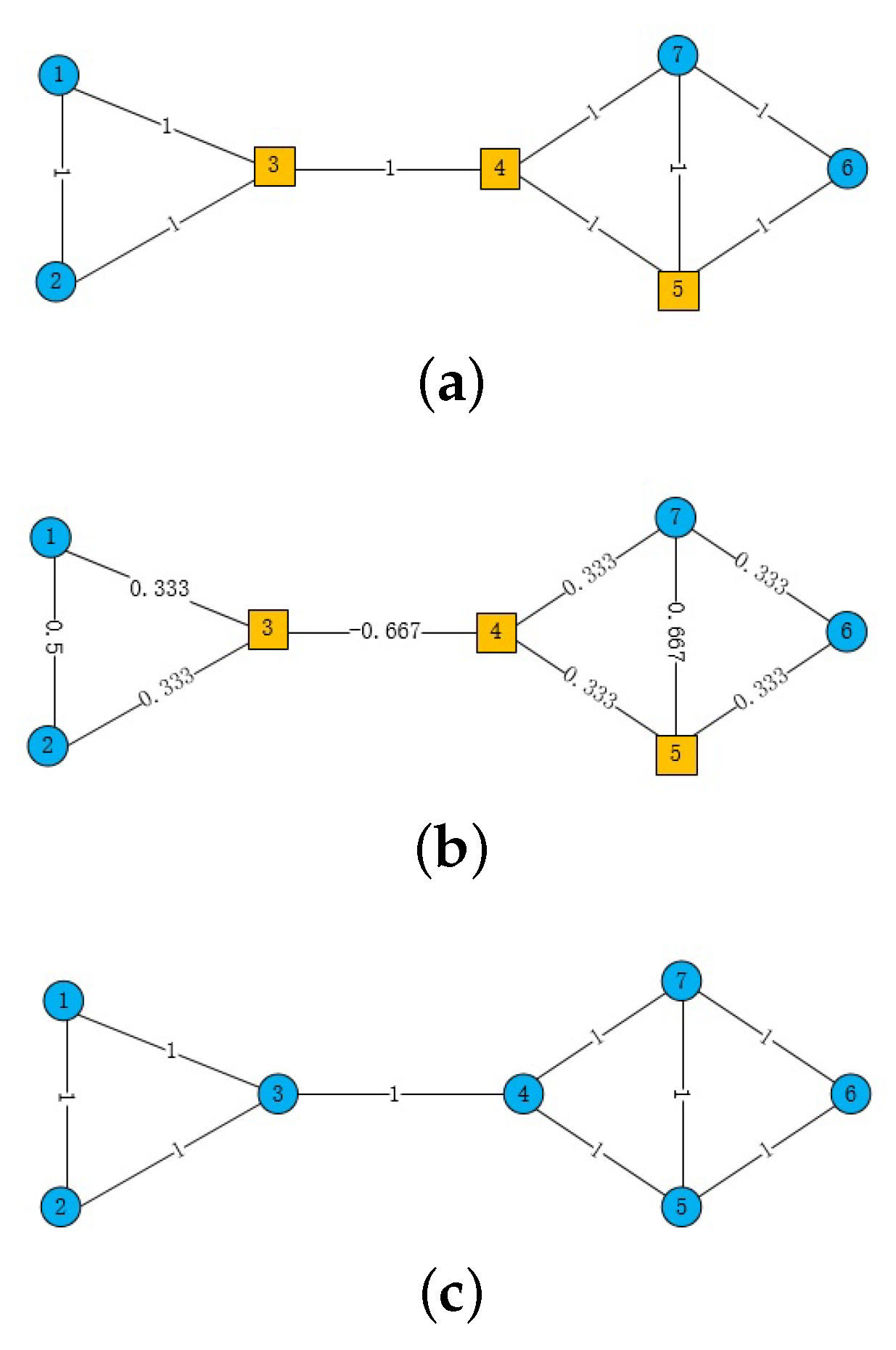
We first consider how the structural information and attribute information can be fused to be more effective and more consistent with the real situation expressed by the data. Let us first take a close look at the three graphs in Figure 1, where the blue circles and the yellow squares at the nodes represent two different attributes in the attributed network. The network shown in Figure 1a consists of 7 nodes, and the weights of the edges are 1. Figure 1b show the same network as Figure 1a, except that the weights of the edges are replaced by the Ricci curvatures of the edges. Figure 1c represents another network where all nodes have the same attributes. DANE [27] inputs topological data and attribute data into two autoencoders, which have their own loss functions for training, and then uses the hidden layer representations of the autoencoders to establish the correlation between the structural information and attribute information for fusion. However, we can see from Figure 1a that, if the attribute information is expressed by the network structure, it does not form a connected graph, which is very different from the network topology. Similarly, in Figure 1c, if a network is constructed by attributes, it is a complete graph that is very different from the network topology. Hence, the idea of looking separately for representations of structures and properties and then merging them does not work very well. As with DANE [27] and ANRL [20], our model uses an autoencoder module. However, we do not process the two heterogeneous information types separately as DANE does, nor do we fuse the structural and attribute information as ANRL does by using an autoencoder to reconstruct the target neighbors. We adopt the way of aggregation attribute features in RCGCN [30]; that is to say, we integrate aggregation layers in the autoencoder for the fusion of structural information and attribute information, rather than input the two types of heterogeneous data into the autoencoder, hoping to achieve fusion only with the help of the autoencoder. According to the analysis conducted by RCGCN, the Ricci curvature is better than the original adjacency matrix for the aggregation of node attributes. The reason is that, as shown in Figure 1b, the Ricci curvature can better distinguish the strength of the connection relationship in the network structure and can distinguish the meso structure of the network, namely, community. For example, the curvature of edge (3,4) in Figure 1a is −0.667, which is a characteristic property of the Ricci curvature, that is, the curvatures of edges between communities are negative. Of course, RCGCN, like GCN, uses semi-supervised learning, while, here, we are going to conduct unsupervised learning.

Since hyperbolic geometry has advantages in representing hierarchical data, and the Ricci curvature can reflect the geometric characteristics of the underlying space where the network is located, we consider adding these elements into the autoencoder module of our model. First, we introduce the sigmoid function commonly used in neural networks, namely,

$$\tau \left(x\right)=\frac{1}{1+e^{-x}}.$$

(18)

Let A represent the adjacency matrix of the network, and C represent the curvature matrix, where the elements are the values of the Ricci curvature of the edges processed by the sigmoid function. Let $S_R^{+}\left(v\right)={\displaystyle \sum _{u\in \mathsf{\Gamma }\left(v\right)}}{c}_{uv}$, where $c_{uv}$ is equal to $\tau \left({\overline{c}}_{uv}\right)$ and ${\overline{c}}_{uv}$ is the Ricci curvature of the edge $(u,v)$. Let us define the matrix S as being equal to $diag(\tau \left(S_R^{+}\left(v_1\right)\right),\cdots ,\tau \left(S_R^{+}\left(v_n\right)\right))$, where $v_1,\cdots ,v_n$ are all nodes in the network. Consequently, we can define the matrix F for fusion as follows:

$$F={\omega }_0·A+{\omega }_1·C+{\omega }_2·S.$$

(19)

In order to avoid the influence of the numerical size on the algorithm, F is normalized. Meanwhile, for the convenience of expression, the normalized aggregation matrix is still denoted as F.

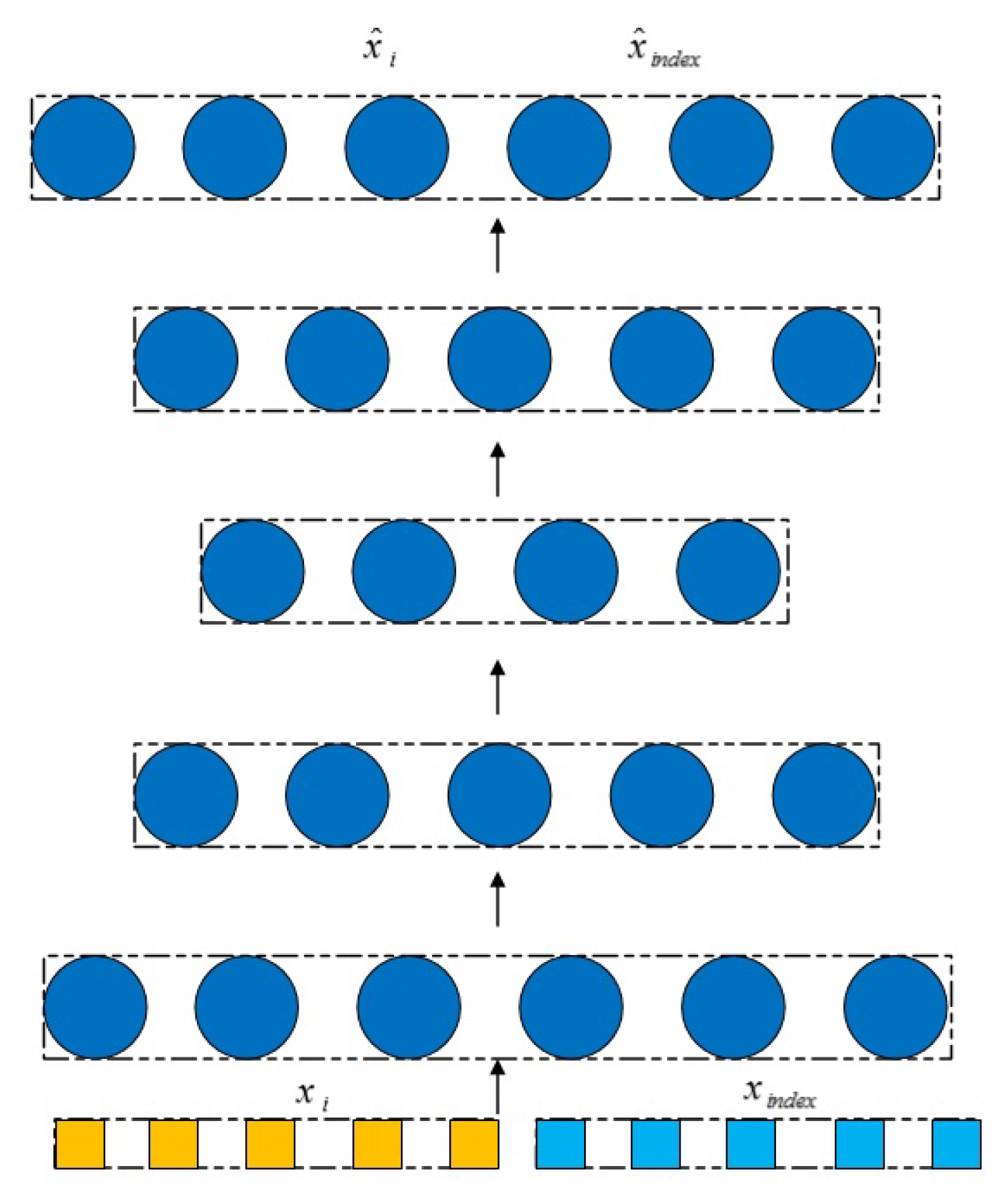
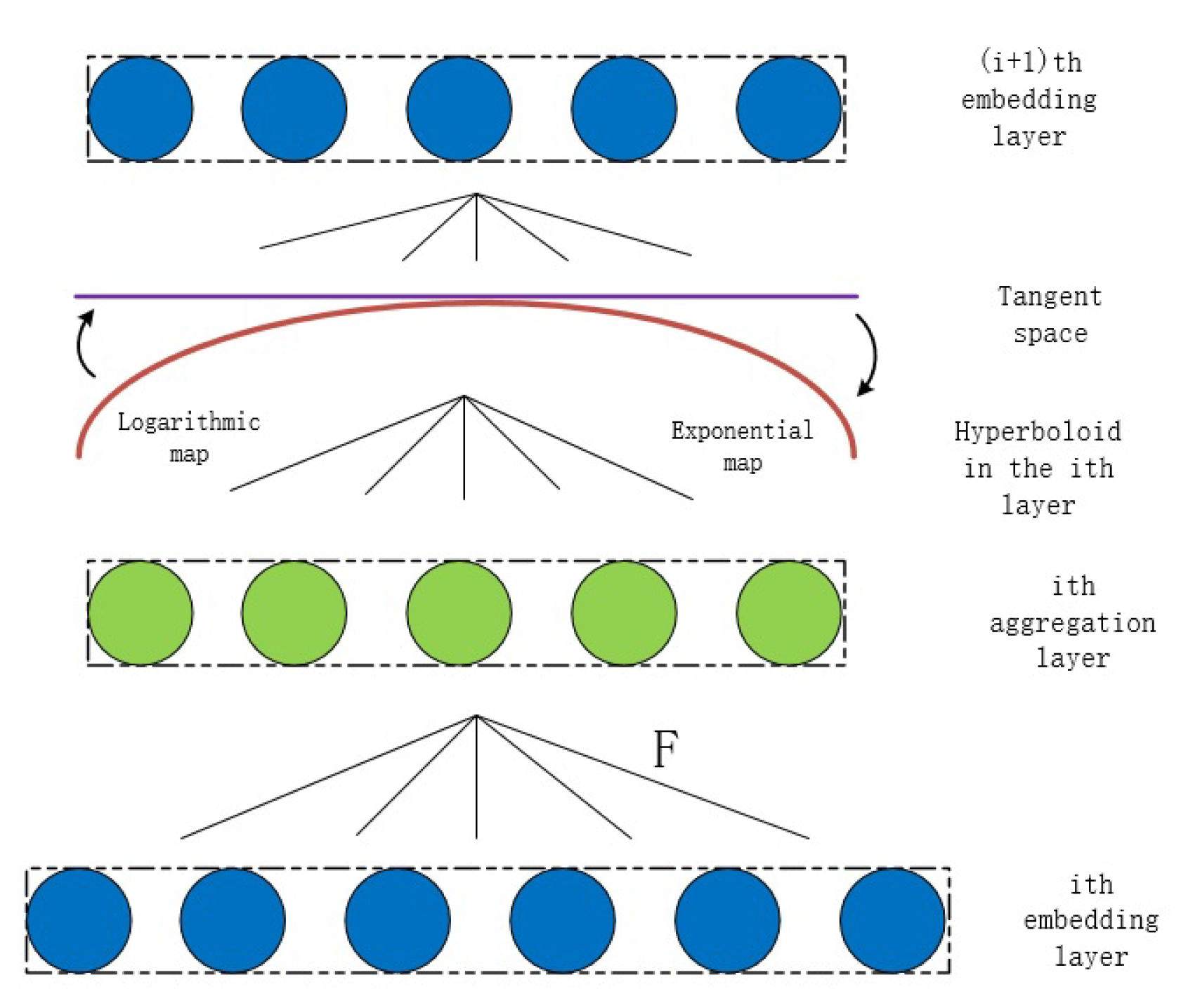
The autoencoder module we adopted is shown in Figure 2. This autoencoder has a total of 5 layers from the input layer to the output layer. The representations of the nodes in the hidden layer are used in the skip-gram module. The attribute data are fed into the autoencoder module in two ways. One is the randomly selected attribute data inputted in batches, denoted as $x_i$. The other is the selected partial attribute data related to the skip-gram module, denoted as $x_{index}$, which will be explained in detail in the section of the introduction to the skip-gram module. It is worth noting that, unlike traditional autoencoders, the representations of layer l in the autoencoder of our model are not directly multiplied by the weight matrix to obtain the representations of layer $l+1$. As shown in Figure 3, an aggregation layer based on the Ricci curvature is inserted between two adjacent layers in our autoencoder module, and the aggregation matrix is shown in Equation (19). After the aggregation layer, there is a hyperbolic embedding layer, which uses a hyperboloid manifold. The operations on the hyperbolic embedding layer need to combine the tangent space of the hyperboloid manifold, and the operations often used include an exponential map and a logarithmic map.

We use X to represent the matrix formed by the attribute vector $x_i$ or $x_{index}$, which is the input of the autoencoder. Specifically, we use $Z^{\left(l\right)}$ to represent the node representations at layer l of the autoencoder, and then we give the derivation of the node representations at layer $l+1$. First, we take $Z^{\left(l\right)}$ as the input of layer l of the autoencoder, fuse it with an aggregation matrix F, multiply it by the weight matrix $W^{\left(l\right)}$ in the Euclidean space, and then map it to a hyperbid manifold, i.e.,

$$hyper{m}^{\left(l\right)}=Ex{p}_o\left(F{Z}^{\left(l\right)}{W}^{\left(l\right)}\right).$$

(20)

Next, the bias vector in the Euclidean space is first projected to the tangent space at the origin of the hyperboloid manifold, and then it is mapped to the hyperboloid manifold by an exponential map, i.e.,

$$hyper{b}^{\left(l\right)}=Ex{p}_o\left(Pro{j}_{R^{n+1}\to T_o{H}^n}\left(b^{\left(l\right)}\right)\right).$$

(21)

Then, we perform the addition operation on the two quantities in Equations (20) and (21) according to Equation (12), and the results are the points in the hyperbolic space, which are pulled back to the Euclidean space, namely, the tangent space, through the logarithmic map:

$$Z^{(l+1)}=\sigma \left(lo{g}_o(hyper{m}^{\left(l\right)}\oplus hyper{b}^{\left(l\right)})\right).$$

(22)

where $\sigma (·)$ represents the activation function. Note that $Z^{\left(0\right)}$ is the attribute matrix X as the input.

Let ${\widehat{x}}_i$ and ${\widehat{x}}_{index}$ be the reconstructed representations obtained after inputting attribute vectors $x_i$ and $x_{index}$ into the autoencoder, respectively. The training goal of the autoencoder is to make the reconstructed attribute vectors close enough to the input attribute vectors. The matrix forms for $x_i$, $x_{index}$, ${\widehat{x}}_i$, and ${\widehat{x}}_{index}$ are X, $X_{index}$, $\widehat{X}$, and ${\widehat{X}}_{index}$, respectively. Hence, the autoencoder loss in our model is set to

$$L_{ae}={\alpha }_0\parallel X-\widehat{X}{\parallel }_2^2+{\alpha }_1\parallel X_{index}-{\widehat{X}}_{index}{\parallel }_2^2.$$

(23)

where ${\parallel ·\parallel }_2$ is the Euclidean norm.

3.3. Skip-Gram Model Based on Ricci Curvature

One of the basic ideas of network embedding is that similar nodes should be close to each other in the embedded space, while dissimilar nodes should be far away. Purely from the perspective of network topology, some works define the similarity according to the neighborhood, that is, they believe that the nodes in the same neighborhood should be similar. The definitions of neighborhood are different in different literature studies. It can be composed of the direct neighbors of the target node, or it can be composed of the first-order neighbors and second-order neighbors of the target node. In some works, sampling is carried out by random walks starting from the target node, and the node pairs obtained by sampling are considered to be similar. This similarity actually reflects the structural information of the network. After these similar node pairs are obtained by the method of random walks, they are input into the skip-gram model for training, and the representations of nodes are obtained.

Take the network in Figure 1a as an example, where we only consider the network structure without considering node attributes. In general, random walks are carried out according to the weights of the edges. Note that the weights of the edges in this network are all 1. Assume that a random walk arrives at node 3 and then decides which node to go to next. According to the traditional decision method of random walk, it is equally possible to choose nodes 1, 2, and 4 in the next step. However, we observe that nodes 1, 2, 3 form one community, while nodes 4, 5, 6, 7 form another community. Considering the community structure, the possibility of selecting node 4 in the next step is less than the possibility of selecting node 1 or node 2 because node 4 and node 3 are not in the same community, while node 3 is in the same community as node 1 and node 2. In other words, if the random walk can reflect the community structure, that is, the meso structure of the network, it can more truly reflect the network structure. The network in Figure 1b corresponds to the network in Figure 1a, and the weights of its edges are the Ricci curvatures of the network’s edges in Figure 1a. As can be seen from Figure 1b, the Ricci curvature of edge (3,4) is −0.667, which is smaller than the Ricci curvature of edge (1,3) and edge (2,3). Therefore, if the random walks are carried out not simply according to the weights of the edges, but according to the Ricci curvatures of the edges, then in the previous problem, starting from node 3, the possibility of selecting node 4 in the next step is less than the possibility of selecting nodes 1 and 2. Consequently, the Ricci curvatures of edges can better reflect the network structure than the weights of edges. In the algorithm, considering that Ricci curvatures have negative values, they are not easy to deal with, so we use a sigmoid function to transform the Ricci curvatures.

It is assumed that $C_{pairs}$ are node pairs sampled by a random walk based on the Ricci curvature. Node pairs in this set are considered to be similar, while other node pairs not in this set are considered to be dissimilar. Let $(v_{index},v_{id})$ be any node pair in set $C_{pairs}$. As mentioned in the previous subsection, the attribute $x_{index}$ corresponding to node $v_{index}$ is input into the autoencoder to obtain the reconstructed representation ${\widehat{x}}_{index}$. The representation of node $v_{index}$ in the most intermediate hidden layer of the autoencoder is denoted as $z_{index}$, which is the representation obtained by integrating the structure and attribute information in the neighborhood of node $v_{index}$. Since $(v_{index},v_{id})$ is a similar node pair, we adopt the processing method in ANRL to further integrate attribute information and structural information in the skip-gram module. We use the following conditional probability to express the similarity of node pairs $(v_{index},v_{id})$:

$$p\left(v_{id}\right|z_{index})=\frac{exp\left(v_{id}^{\prime T}{z}_{index}\right)}{{\displaystyle \sum _{j=1}^n}exp\left(v_j^{\prime T}{z}_{index}\right)},$$

(24)

where $v_{index}^{\prime }$ is the representation of node $v_{index}$ when it is treated as a context node. Since the calculation of the denominator of Equation (24) involves the whole network, the calculation amount is too large; therefore, we adopt the negative sampling technique in [31] to reduce the calculation amount. Specifically, for a positive sample node pair $(v_{index},v_{id})$, we have the following loss function:

$$log\tau \left(v_{id}^{\prime T}{z}_{index}\right)+{\mathbb{E}}_{v_n\sim P_n\left(v\right)}\left[log\tau (-v_n^{\prime T}{z}_{index})\right],$$

(25)

where $P_n\left(v\right)\propto d_v^{\frac{3}{4}}$ is the same as [31], and $d_v$ is the degree of node v.

Consequently, the corresponding loss function of the skip-gram module is

$$L_{sg}=\sum _{(v_{index},v_{id})\in C_{pairs}}[log\tau \left(v_{id}^{\prime T}{z}_{index}\right)+{\mathbb{E}}_{v_n\sim P_n\left(v\right)}\left[log\tau (-v_n^{\prime T}{z}_{index})\right]].$$

(26)

3.4. RHAE Architecture

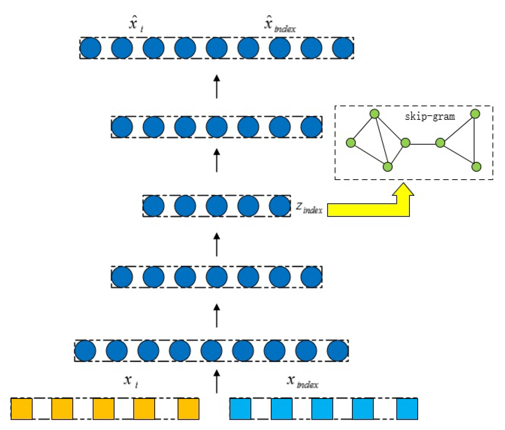
As shown in Figure 4, the RHAE model adopts two modules, namely, the autoencoder module and the skip-gram module. These two modules have the function of integrating structural information and attribute information of the network, but the way of fusion is different. The autoencoder module aggregates the information of two heterogeneous sources mainly by means of the aggregation matrix based on the Ricci curvature and hyperbolic geometry, while the skip-gram module explores the similarity of the nodes in the generalized neighborhood of the target node mainly by means of random walks based on the Ricci curvature, in order to realize the expected fusion. The two modules are coupled together. In the process of model training, the parameters of the two modules influence each other, in order to realize the purpose of learning node representations jointly.

According to previous analysis, the objective function of the RHAE model is defined as a linear combination of the loss functions of two modules, and a regular term related to the network weight matrix is added at the same time, i.e.,

$$L=L_{ae}+{\beta }_0{L}_{sg}+{\beta }_1{L}_{reg}=L_{ae}+{\beta }_0{L}_{sg}+{\beta }_1\sum _{l=1}^N{\parallel W^{\left(l\right)}\parallel }_F^2,$$

(27)

where N is the number of autoencoder layers, $W^{\left(l\right)}$ is the l-th weight matrices of the autoencoder, ${\beta }_0$ is the hyperparameter used to balance the corresponding loss between the two modules, and ${\beta }_1$ is the regular term coefficient.

4. Experiment

In this section, in order to evaluate the effectiveness of our RHAE model, we conduct a number of experiments to compare it with some baseline approaches on the benchmark datasets.

4.1. Datasets

Five datasets are used in our experiments, namely, Cora, Wiki, Wisconsin, Cornell, and Texas. The statistics for these datasets are listed in

Table 1. Dataset statistics.

Dataset	Nodes	Edges	Classes	Features
Cora	2708	5278	7	1433
Wiki	2405	17,981	17	4973
Wisconsin	251	499	5	1703
Cornell	183	295	5	1703
Texas	183	309	5	1703

.

Cora is a network of citation datasets with 2708 nodes and 5278 edges. The nodes of the network represent the papers in the dataset, and the edges represent the reference relationships between the papers. The attribute features of nodes are the TFIDF vectors of the papers. Papers in the dataset are divided into seven categories according to their topics, and node labels are the corresponding categories of papers.

Wiki is a network constructed from a dataset of web pages. Nodes in the network correspond to web pages, and edges correspond to hyperlinks between web pages. The dataset contains 2405 web pages with 17,981 hyperlinks between them. The attribute features of the nodes in the network are the TFIDF vectors of the web pages. These web pages are divided into 17 categories, which, like Cora, are used as nodes’ labels.

Wisconsin, Cornell, and Texas are three subsets of WebKB, which is a dataset made up of web pages. These datasets construct the networks in which nodes represent web pages and edges represent hyperlinks between pages. The numbers of nodes and edges in these three datasets are shown in Table 1. The node features are the bag-of-words vectors of the corresponding web pages, and the node labels represent the categories of the corresponding web pages. The web pages in the three datasets are grouped into five categories.

4.2. Baseline Methods Setup

Our approach is unsupervised, and therefore we chose some unsupervised methods as baselines. The node classification performance is used as an evaluation metric to compare our method with the baselines. The baseline methods are described in detail below.

Deepwalk [1]: This method obtains node sequences through truncated random walks of each node in the network and then inputs these node sequences into the skip-gram model for training. The skip-gram model obtains node representations by maximizing the probability of co-occurrence node pairs appearing in the moving window. The super parameters of the model are set as follows: the length of the random walk is 80, the number of walks from each node is 10, and the window size is 10.

Node2vec [32]: This method explores the neighborhood of each node through second-order random walks and thus obtains similar node pairs. Then, it obtains network embedding by maximizing the co-occurrence probability of similar node pairs. Its super parameters p and q are set to 1.

DANE [27]: This method uses two autoencoders to process topological information and attribute information and carries out network embedding learning under the correlation constraint of hidden representations.

ANRL [20]: This method uses the autoencoder module to reconstruct the neighbor of the target node; meanwhile, it uses the skip-gram module to capture the network structure. Through the combination of the two modules, it can obtain the representations of the network nodes which integrate the structural information and the attribute information.

4.3. Node Classification

We use node classification to evaluate the performance of our model, RHAE. We randomly selected some nodes with labels for training and the rest for testing. To examine model performance more fully, we incrementally increased the percentage of labeled nodes used for training from 10% to 50% while recording performance data for both our model and the baseline approaches. Macro-F1 and Micro-F1 are used as evaluation metrics for node classification performance. The epoch of the experiments is 200, and each result is the average value obtained by repeated running for 10 times. For the datasets of Wisconsin, Cornell, and Texas, the embedding dimension of all models is set to 16, while for the dataset of Cora, the embedding dimension of all models is set to 128. For the dataset of Wiki, the embedding dimension of all models is set to 128, except for Deepwalk and Node2vec, which have an embedding dimension of 16 because for Deepwalk and Node2vec, the performance is better with an embedding dimension of 16. For our model, RHAE, on each dataset, the hyperparameters of Equations (19), (23) and (27) are, respectively, set as follows: for the dataset of Cora, ${\omega }_0$ = 1.0, ${\omega }_1$ = 0.5, ${\omega }_2$ = 1.0, ${\alpha }_0$ = 1.0, ${\alpha }_1$ = 0.01, ${\beta }_0$ = 0.1, ${\beta }_1$ = 1.0; for the dataset of Wiki, ${\omega }_0$ = 0.02, ${\omega }_1$ = 0.04, ${\omega }_2$ = 1.0, ${\alpha }_0$ = 1.0, ${\alpha }_1$ = 0.01, ${\beta }_0$ = 0.1, ${\beta }_1$ = 1.0; for the dataset of Wisconsin, ${\omega }_0$ = 0.0012, ${\omega }_1$ = 0.004, ${\omega }_2$ = 1.0, ${\alpha }_0$ = 1.0, ${\alpha }_1$ = 0.05, ${\beta }_0$ = 0.1, ${\beta }_1$ = 1.0; for the dataset of Cornell, ${\omega }_0$ = 0.003, ${\omega }_1$ = 0.0035, ${\omega }_2$ = 1.0, ${\alpha }_0$ = 1.0, ${\alpha }_1$ = 0.01, ${\beta }_0$ = 0.1, ${\beta }_1$ = 1.0; and for the dataset of Texas, ${\omega }_0$ = 0.003, ${\omega }_1$ = 0.0035, ${\omega }_2$ = 1.0, ${\alpha }_0$ = 1.0, ${\alpha }_1$ = 0.01, ${\beta }_0$ = 0.2, ${\beta }_1$ = 1.0.

Table 2. Node classification accuracy of Cora.

Methods	The Percentage of Labeled Nodes
	10%		20%		30%		40%		50%
	Macro-F1	Macro-F1	Macro-F1	Macro-F1	Macro-F1	Macro-F1	Macro-F1	Macro-F1	Macro-F1	Macro-F1
DeepWalk	63.32	71.90	71.83	76.29	78.02	78.99	78.26	78.68	79.91	80.53
Node2vec	63.32	71.89	72.88	76.46	78.12	79.08	78.04	78.73	79.64	80.37
DANE	76.48	78.11	76.88	78.77	77.94	79.95	78.64	80.65	78.64	80.91
ANRL	68.16	71.13	70.85	73.28	72.36	74.75	72.93	75.13	73.36	75.60
RHAE	80.13	81.50	82.64	83.83	84.01	85.13	84.77	85.86	85.29	86.27

,

Table 3. Node classification accuracy of Wiki.

Methods	The Percentage of Labeled Nodes
	10%		20%		30%		40%		50%
	Macro-F1	Macro-F1	Macro-F1	Macro-F1	Macro-F1	Macro-F1	Macro-F1	Macro-F1	Macro-F1	Macro-F1
DeepWalk	37.05	56.51	41.13	60.43	42.87	62.39	43.70	63.06	45.32	63.78
Node2vec	36.87	56.33	40.52	60.51	43.78	61.54	44.42	63.76	45.58	63.97
DANE	57.23	72.36	61.12	75.58	63.12	77.20	68.07	78.63	68.60	78.93
ANRL	43.97	58.25	47.69	60.62	50.00	62.98	52.66	64.80	53.22	65.60
RHAE	62.23	74.63	68.14	77.91	70.59	79.22	71.94	80.12	73.68	81.07

,

Table 4. Node classification accuracy of Wisconsin.

Methods	The Percentage of Labeled Nodes
	10%		20%		30%		40%		50%
	Macro-F1	Macro-F1	Macro-F1	Macro-F1	Macro-F1	Macro-F1	Macro-F1	Macro-F1	Macro-F1	Macro-F1
DeepWalk	15.09	44.51	15.08	47.36	15.99	46.99	18.91	48.74	17.09	47.30
Node2vec	14.05	45.09	15.78	46.32	17.94	48.01	17.86	48.48	18.87	48.89
DANE	49.25	71.28	51.23	74.18	52.27	74.66	51.76	75.30	52.00	73.49
ANRL	33.39	53.03	37.80	58.02	39.94	60.44	41.06	60.54	42.01	62.06
RHAE	49.66	73.80	56.82	77.24	62.06	80.84	64.36	82.23	65.11	83.06

,

Table 5. Node classification accuracy of Cornell.

Methods	The Percentage of Labeled Nodes
	10%		20%		30%		40%		50%
	Macro-F1	Macro-F1	Macro-F1	Macro-F1	Macro-F1	Macro-F1	Macro-F1	Macro-F1	Macro-F1	Macro-F1
DeepWalk	14.57	55.09	15.34	55.51	15.45	55.12	15.37	53.64	16.53	54.35
Node2vec	14.53	54.79	15.03	54.56	14.94	55.19	15.87	56.18	14.45	54.46
DANE	37.07	60.73	40.17	69.53	44.85	73.18	42.83	71.55	46.00	74.13
ANRL	27.83	53.96	34.09	58.84	35.74	59.41	41.95	63.13	44.12	63.39
RHAE	42.12	69.25	52.04	75.45	57.15	77.83	59.63	78.17	61.63	78.39

and

Table 6. Node classification accuracy of Texas.

Methods	The Percentage of Labeled Nodes
	10%		20%		30%		40%		50%
	Macro-F1	Macro-F1	Macro-F1	Macro-F1	Macro-F1	Macro-F1	Macro-F1	Macro-F1	Macro-F1	Macro-F1
DeepWalk	15.17	54.48	17.05	55.51	15.67	55.19	16.75	55.82	15.74	55.65
Node2vec	14.07	54.30	15.50	55.31	16.22	55.58	14.61	53.45	16.32	53.59
DANE	32.76	54.00	38.21	68.98	46.11	73.56	35.05	67.64	41.81	71.63
ANRL	30.52	56.13	37.45	62.11	40.83	63.92	42.35	66.06	45.39	66.60
RHAE	40.93	68.33	52.31	75.06	57.80	77.50	60.13	79.31	62.61	78.59

give the results of node classification, with the best performance indicated in bold. As you can see from the results in these tables, the node classification performance of Deepwalk and Node2vec is lower than that of the other methods on datasets other than Cora. The reason is that Deepwalk and Node2vec only utilize network structure information, while other methods utilize both structure information and attribute information. On the Cora dataset, the method using only structural information can match the node classification performance of ANRL, which may be due to the characteristics of the Cora dataset itself, that is, structural information makes a greater contribution to the classification performance than attribute information. In addition, our model, RHAE, achieves optimal performance on all datasets. It proves that RHAE can make full use of the network geometry to integrate attribute information and structural information to improve the performance of the model.

4.4. The Effect of Embedding Dimension

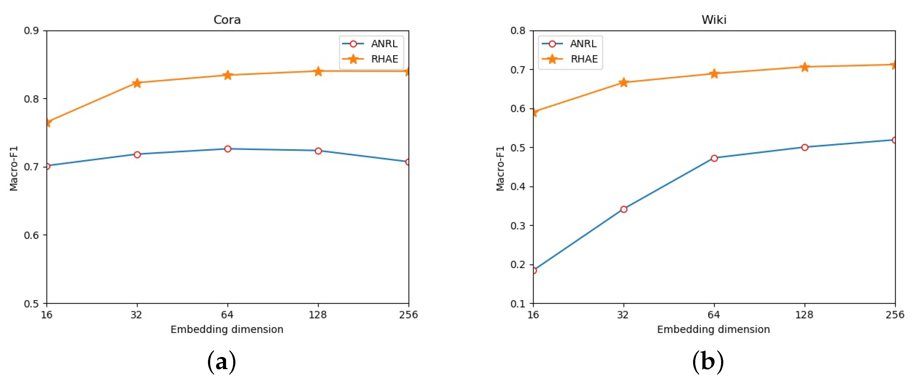
The encoder module and skip-gram module are adopted in the basic architecture of our RHAE model and ANRL. In order to better compare the two models, we changed the embedding dimensions to compare the node classification performance of the two models while keeping other parameters unchanged, that is, the same setting as in Section 4.3. The datasets used here include Cora and Wiki. All the results are shown in Figure 5.

4.5. Training Time Comparison

RHAE is inspired by ANRL. Now, let us compare the training time taken by the two models. We implement the algorithm RHAE using the TensorFlow framework. All experiments in this paper were conducted on a CPU, using a notebook computer with an Intel Core i7 2.8 GHz processor and 8 G RAM. Figure 6 shows the results of the training time comparison between the two models on each dataset. RHAE takes more training time than ANRL, mainly because RHAE has more operations, such as calculating the Ricci curvature.

5. Conclusions and Future Work

In this paper, we discussed the representation learning of an attributed network from the point of view of non-Euclidean geometry. Our model, known as RHAE, utilizes two geometric tools in non-Euclidean geometry, namely, hyperbolic geometry and the Ricci curvature. Compared with Euclidean geometry, hyperbolic geometry has advantages in modeling hierarchical data such as networks. The Ricci curvature can give different importance to the neighbor nodes of the target node, that is, it can identify the difference in network structure well. We improved the performance of the model by incorporating the above non-Euclidian geometry into the autoencoder module and skip-gram module. Experimental results on benchmark datasets show that our algorithm performs better than other baseline methods. In the future, we will improve our model in the following aspects: (1) we will consider adding global structural information to improve model performance; (2) we will try to extend this model to the case of heterogeneous networks.

References

- Perozzi, B.; Al-Rfou, R.; Skiena, S. Deepwalk: Online learning of social representations. In Proceedings of the 20th ACM SIGKDD International Conference on Knowledge Discovery and Data Mining, New York, NY, USA, 24–27 August 2014; pp. 701–710. [Google Scholar] [CrossRef] [Green Version]
- Tang, J.; Qu, M.; Wang, M.; Zhang, M.; Yan, J.; Mei, Q. Line: Large-scale information network embedding. In Proceedings of the 24th International Conference on World Wide Web, Florence, Italy, 18–22 May 2015; pp. 1067–1077. [Google Scholar] [CrossRef] [Green Version]
- Zhang, D.; Yin, J.; Zhu, X.; Zhang, C. SINE: Scalable incomplete network embedding. In Proceedings of the 2018 IEEE International Conference on Data Mining (ICDM), Singapore, 17–20 November 2018; pp. 737–746. [Google Scholar]
- Galland, A.; Lelarge, M. Invariant Embedding for Graph Classification. In ICML 2019 Workshop on Learning and Reasoning with Graph-Structured Data; HAL: Long Beach, CA, USA, 2019; Available online: https://hal.archives-ouvertes.fr/hal-02947290/document (accessed on 15 May 2021).
- Tixier, A.J.P.; Nikolentzos, G.; Meladianos, P.; Vazirgiannis, M. Graph classification with 2d convolutional neural networks. In International Conference on Artificial Neural Networks; Springer: Cham, Switzerland, 2019; pp. 578–593. [Google Scholar]
- Wen, Y.; Guo, L.; Chen, Z.; Ma, J. Network embedding based recommendation method in social networks. In Proceedings of the WWW’18: Companion Proceedings of the Web Conference 2018, Lyon, France, 23–27 April 2018; pp. 11–12. [Google Scholar] [CrossRef] [Green Version]
- Shi, C.; Hu, B.; Zhao, W.X.; Philip, S.Y. Heterogeneous information network embedding for recommendation. IEEE Trans. Knowl. Data Eng. 2018, 31, 357–370. [Google Scholar] [CrossRef] [Green Version]
- Cavallari, S.; Zheng, V.W.; Cai, H.; Chang, K.C.C.; Cambria, E. Learning community embedding with community detection and node embedding on graphs. In Proceedings of the 2017 ACM on Conference on Information and Knowledge Management, Singapore, 6–10 November 2017; pp. 377–386. [Google Scholar]
- Jin, D.; You, X.; Li, W.; He, D.; Cui, P.; Fogelman-Soulié, F.; Chakraborty, T. Incorporating network embedding into markov random field for better community detection. In Proceedings of the AAAI Conference on Artificial Intelligence, Honolulu, HI, USA, 27 January–1 February 2019; Volume 33, pp. 160–167. [Google Scholar]
- Wang, D.; Cui, P.; Zhu, W. Structural deep network embedding. In Proceedings of the 22nd ACM SIGKDD International Conference on Knowledge Discovery and Data Mining, San Francisco, CA, USA, 13–17 August 2016; ACM: San Francisco, CA, USA, 2016; pp. 1225–1234. [Google Scholar] [CrossRef]
- Cao, S.; Lu, W.; Xu, Q. Deep neural networks for learning graph representations. In Proceedings of the AAAI Conference on Artificial Intelligence, Phoenix, AZ, USA, 12–17 February 2016; Volume 30. [Google Scholar]
- Zhang, Z.; Cui, P.; Wang, X.; Pei, J.; Yao, X.; Zhu, W. Arbitrary-order proximity preserved network embedding. In Proceedings of the 24th ACM SIGKDD International Conference on Knowledge Discovery & Data Mining, London, UK, 19–23 August 2018; pp. 2778–2786. [Google Scholar]
- Keikha, M.M.; Rahgozar, M.; Asadpour, M. Community aware random walk for network embedding. Knowl. Based Syst. 2018, 148, 47–54. [Google Scholar] [CrossRef] [Green Version]
- Yang, S.; Yang, B. Enhanced network embedding with text information. In Proceedings of the 2018 24th International Conference on Pattern Recognition (ICPR), Beijing, China, 20–24 August 2018; pp. 326–331. [Google Scholar]
- Bandyopadhyay, S.; Biswas, A.; Kara, H.; Murty, M. A Multilayered Informative Random Walk for Attributed Social Network Embedding. Front. Artif. Intell. Appl. 2020, 325, 1738–1745. [Google Scholar]
- Shen, E.; Cao, Z.; Zou, C.; Wang, J. Flexible Attributed Network Embedding. arXiv 2018, arXiv:1811.10789. [Google Scholar]
- Sala, F.; De Sa, C.; Gu, A.; Ré, C. Representation tradeoffs for hyperbolic embeddings. In Proceedings of the International Conference on Machine Learning, Stockholm, Sweden, 10–15 July 2018; pp. 4460–4469. [Google Scholar]
- Klimovskaia, A.; Lopez-Paz, D.; Bottou, L.; Nickel, M. Poincaré maps for analyzing complex hierarchies in single-cell data. Nat. Commun. 2020, 11, 1–9. [Google Scholar] [CrossRef]
- Chami, I.; Ying, R.; Ré, C.; Leskovec, J. Hyperbolic graph convolutional neural networks. Adv. Neural Inf. Process. Syst. 2019, 32, 4869. [Google Scholar] [PubMed]
- Zhang, Z.; Yang, H.; Bu, J.; Zhou, S.; Yu, P.; Zhang, J.; Ester, M.; Wang, C. ANRL: Attributed Network Representation Learning via Deep Neural Networks. In IJCAI; 2018; Volume 18, pp. 3155–3161. Available online: https://www.ijcai.org/Proceedings/2018/0438.pdf (accessed on 15 May 2021).
- Krioukov, D.; Papadopoulos, F.; Kitsak, M.; Vahdat, A.; Boguná, M. Hyperbolic geometry of complex networks. Phys. Rev. E 2010, 82, 036106. [Google Scholar] [CrossRef] [PubMed] [Green Version]
- Leimeister, M.; Wilson, B.J. Skip-gram word embeddings in hyperbolic space. arXiv 2018, arXiv:1809.01498. [Google Scholar]
- Ollivier, Y. Ricci curvature of Markov chains on metric spaces. J. Funct. Anal. 2009, 256, 810–864. [Google Scholar] [CrossRef] [Green Version]
- Lin, Y.; Lu, L.; Yau, S.T. Ricci curvature of graphs. Tohoku Math. J. Second Ser. 2011, 63, 605–627. [Google Scholar] [CrossRef]
- Jost, J.; Liu, S. Ollivier’s Ricci curvature, local clustering and curvature-dimension inequalities on graphs. Discret. Comput. Geom. 2014, 51, 300–322. [Google Scholar] [CrossRef]
- Pouryahya, M.; Mathews, J.; Tannenbaum, A. Comparing three notions of discrete ricci curvature on biological networks. arXiv 2017, arXiv:1712.02943. [Google Scholar]
- Gao, H.; Huang, H. Deep attributed network embedding. In Proceedings of the Twenty-Seventh International Joint Conference on Artificial Intelligence (IJCAI)), Stockholm, Sweden, 13–19 July 2018. [Google Scholar]
- Liao, L.; He, X.; Zhang, H.; Chua, T.S. Attributed social network embedding. IEEE Trans. Knowl. Data Eng. 2018, 30, 2257–2270. [Google Scholar] [CrossRef] [Green Version]
- Cen, K.; Shen, H.; Gao, J.; Cao, Q.; Xu, B.; Cheng, X. ANAE: Learning Node Context Representation for Attributed Network Embedding. arXiv 2019, arXiv:1906.08745. [Google Scholar]
- Wu, W.; Hu, G.; Yu, F. Ricci Curvature-Based Semi-Supervised Learning on an Attributed Network. Entropy 2021, 23, 292. [Google Scholar] [CrossRef] [PubMed]
- Mikolov, T.; Sutskever, I.; Chen, K.; Corrado, G.; Dean, J. Distributed representations of words and phrases and their compositionality. arXiv 2013, arXiv:1310.4546. [Google Scholar]
- Grover, A.; Leskovec, J. node2vec: Scalable feature learning for networks. In Proceedings of the 22nd ACM SIGKDD International Conference on Knowledge Discovery and Data Mining, San Francisco, CA, USA, 13–17 August 2016; pp. 855–864. [Google Scholar] [CrossRef] [Green Version]
Figure 1.
Attributed networks and Ricci curvature. (1) (a) is an undirected nework, which consists of 7 nodes, and the weights of the edges are 1; (b) show the same network as (a), except that the weights of the edges are replaced by the Ricci curvatures of the edges; The blue circles and the yellow squares at the nodes represent two different attributes in these two attributed networks. (2) (c) represents another network where all nodes have the same attributes.
Figure 2.
Illustration of an autoencoder module.
Figure 3.
Description of curvatude-based aggregation layers and hyperbolic embedding layers in autoencoder.
Figure 4.
Figure 5.
The effect of embedding dimension. (a) shows that RHAE’s node classification performance in dimension 16, 32, 64, 128, 256 is better than that of ANRL in Cora dataset. The performance of ANRL peaked at dimension 128 and begin to decline, while the performance of RHAE don’t decline at the above dimensions. (b) shows that on the Wiki dataset, RHAE still performs better than ANRL in the above dimensions, especially in the lower dimensions. This shows that RHAE does indeed capture the true geometry of the network.