
Survival and Reliability Analysis with an Epsilon-Positive Family of Distributions with Applications


1
Facultad de Ingeniería y Ciencias, Universidad Adolfo Ibáñez, Diagonal Las Torres 2640, Peñalolén, Santiago 7941169, Chile
2
Department of Statistics, Oregon State University, 217 Weniger Hall, Corvallis, OR 97331, USA
3
Departamento de Matemática, Facultad de Ciencias Básicas, Universidad de Antofagasta, Antofagasta 1240000, Chile
*
Author to whom correspondence should be addressed.
Symmetry 2021, 13(5), 908; https://0-doi-org.brum.beds.ac.uk/10.3390/sym13050908
Submission received: 25 April 2021
/
Revised: 14 May 2021
/
Accepted: 18 May 2021
/
Published: 20 May 2021
(This article belongs to the Special Issue Symmetric and Asymmetric Distributions: Theoretical Developments and Applications II)
Abstract
:We introduce a new class of distributions called the epsilon–positive family, which can be viewed as generalization of the distributions with positive support. The construction of the epsilon–positive family is motivated by the ideas behind the generation of skew distributions using symmetric kernels. This new class of distributions has as special cases the exponential, Weibull, log–normal, log–logistic and gamma distributions, and it provides an alternative for analyzing reliability and survival data. An interesting feature of the epsilon–positive family is that it can viewed as a finite scale mixture of positive distributions, facilitating the derivation and implementation of EM–type algorithms to obtain maximum likelihood estimates (MLE) with (un)censored data. We illustrate the flexibility of this family to analyze censored and uncensored data using two real examples. One of them was previously discussed in the literature; the second one consists of a new application to model recidivism data of a group of inmates released from the Chilean prisons during 2007. The results show that this new family of distributions has a better performance fitting the data than some common alternatives such as the exponential distribution.
1. Introduction
The statistical analysis of reliability and survival data is an important topic in several areas, including medicine, epidemiology, biology, economics, engineering, and environmental sciences, to name a few. When using a parametric approach, one of the first steps for modeling the data is to choose a suitable distribution that can capture relevant features of the observations of interest. In this context, the gamma and Weibull distributions have become popular choices due to their flexibility that allows for a non-constant hazard rate function and to model skewed data. Although several alternatives were considered to accommodate different cases, researchers have continued to develop extensions and modifications of the standard distributions to increase the flexibility of the models see [1,2,3] for a few examples.
In this paper, we consider a generalization of the distributions with positive support and propose a new family of distributions, called the epsilon–positive family, whose construction is motivated by the ideas behind the generation of skew distributions using symmetric kernels. Specifically, we build upon the ideas from [4], where the authors start with a symmetric around zero distribution f, and define a family of distributions indexed by a parameter as the set of densities of the form
where denotes the indicator function of the set A. Some extensions of this family include epsilon-skew-normal family introduced by [5] and the epsilon–skew–symmetric family introduced by [6], both discussed in some details in [7].
Here, starting with a probability density function g with positive support, we obtain a general class that extends the family of distributions with positive support, and that contains the Weibull, gamma and exponential distributions as special cases, depending on the choice of g. Furthermore, we discuss a stochastic representation and how to obtain maximum likelihood estimators for the members of this family. We also derive the corresponding survival and hazard functions and note that one interesting feature of this new class is that the hazard function is not necessarily constant.
The rest of the paper is organized as follows: in Section 2 we define the epsilon–positive family and obtain the hazard and survival functions, mean residual life and stress-strength parameters for this family. In addition, we discuss maximum likelihood estimation and how to obtain such estimates using an EM-type algorithm for the general case. In Section 3, we focus on one specific member of the family introduced in Section 2, namely epsilon–exponential distribution, and discuss its applicability in the analysis of survival data. In Section 4 we discuss two real data examples and we finish with a brief discussion in Section 5. We include Appendix A and Appendix B with some of the technical details.
2. The Epsilon–Positive Family
Let be a probability density function (pdf) with positive support and parameters . Then, for , the corresponding epsilon–positive (EP) family of distributions is defined as
If a random variable X has the density given in (2), we say that X has an epsilon–positive distribution and write .
Observe that as , and therefore the distribution can be seen as a particular member of the family.
The rth moment of , is given by
where is the rth moment of . From (3) we obtain that the mean, variance, skewness (CS) and kurtosis (CK) coefficients are (respectively)
and
where , , are the first four moments of the random variable .
To draw observations from an epsilon–positive distribution, we first notice that for , if and (independent from Y) satisfies , then .
From this stochastic representation, it follows that we can generate EP random variables according to the Algorithm 1:
| Algorithm 1 Algorithm to generate observations from an epsilon–positive distribution. |
| Require: Initialize the algorithm fixing and |
| 1: Generate Y from and U from |
| 2: if then |
| 3: |
| 4: else |
| 5: |
| 6: end if |
| 7: return |
Finally, observe that the definition in (2) can be easily extended so we can represent the epsilon–positive family as a finite scale mixture of positive distributions. In fact, for any we can write
where , are mixing proportions satisfying , and is some finite subset of ℜ that will typically depend on . For instance, taking and we recover the expression in (2). This representation will be particularly useful in order to obtain maximum likelihood estimates using EM–type algorithms, as we discuss in Section 2.5.
2.1. Reliability Properties
From the definition, we obtain that the survival function for this family is given by
where is the survival function associated with the density . Similarly, the hazard function is given by
where , and is the Mills ratio.
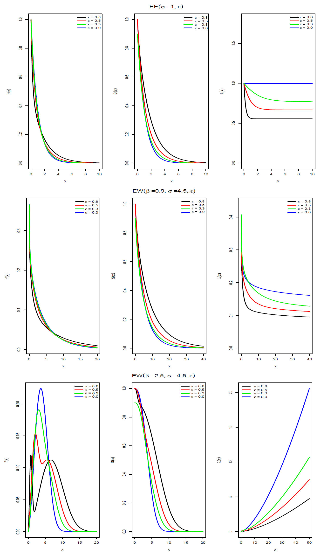
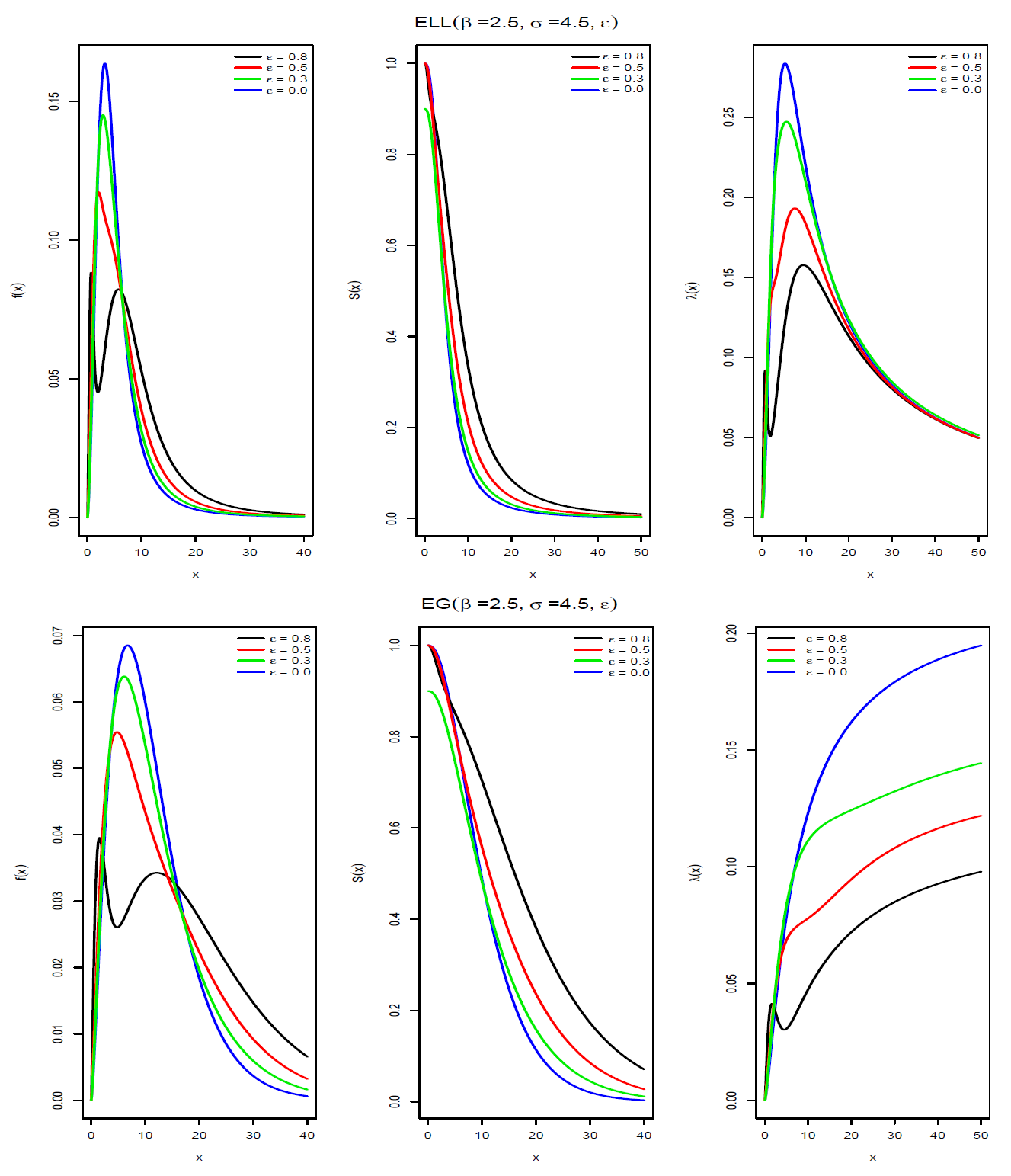
Table 1 shows some examples of the densities that can be extended using the definition of the epsilon–positive family, with the corresponding densities, survival and hazard functions. Figure 1 and Figure 2 show the pdf, survival and hazard functions of the epsilon-exponential, epsilon-Weibull, epsilon-log-logistic and epsilon-gamma distributions. We can see that in the case of the epsilon-Weibull, epsilon-log-logistic and epsilon-gamma distributions a bimodal shape is obtained when the value of the parameter is .
2.2. Mean Residual Life
The mean residual life or life expectancy is an important characteristic of the model. It gives the expected additional lifetime given that a component has survived until time t. For a non-negative continuous random variable the mean residual life () function is defined as
where . The above conditional expectation is given by
Calculation of the integral in (8) is done in the same way as the calculation of the mean. Thus,
Making the changes of variables and we have
where , , and , corresponds to the mean residual life of the random variable . Finally, Equation (7) can be written as
2.3. Stress-Strength Parameter
An important concept in reliability theory is the stress-strength parameter. Let denote the strength of a system or component with a stress . Then, the stress-strength parameter is defined as , which can be viewed as a measure of the system performance. In the next theorem, we look at this quantity when and are independent random variables with epsilon-positive distributions.
Theorem 1.
Suppose and are random variables independently distributed as and , the reliability of the system with stress variable () and strength variable () is given by
where , , , , and , , with independent of .
Proof of Theorem 1.
Making the changes of variables and we have
□
Observe that the same concept can be used to make comparisons between two systems. For example, if and denote instead the lifetimes of systems and respectively, then, a probability would indicate that the system is better than the system in a stochastic sense.
2.4. Maximum Likelihood Estimation
Let be a random sample from an distribution. Then, the maximum likelihood estimator (MLE) of is given by
where is the log–likelihood.
Although the MLE for the family is conceptually straightforward, typically closed form solutions are not available and the MLE need to be obtained numerically. One possibility is the Newton–Raphson algorithm, with iteration equation
where be the current estimate of , denote the vector of first derivatives of , and .
A disadvantage of this approach is that it requires redthe calculation of the second derivatives of the likelihood function and repeated inversion of potentially large matrices, which can be computationally intensive. Instead, we can consider an expectation–maximization (EM) approach see [8] as a general iterative method for data sets with missing (or incomplete) data.
The mixture representation proposed in (4) is particularly useful in order to use an EM–type algorithm to estimate the model parameters, since it provides a hierarchical scheme for the family. Next, we show how to implement maximum likelihood estimation using an EM–type algorithm for the family.
2.5. MLE via the EM Algorithm
From (4), the log–likelihood takes the form,
where the derivatives with respect to and typically lead to a system of equations with no closed form solution. To address this problem, we can “augment” the data using an unobservable matrix , , with elements defined as
where denote the distinct elements of . This way, each row of W contains only one 1 and zero 0, and the (complete) log-likelihood for the augmented data is given by
Then, if we denote by the estimate of at iteration s, and by , the conditional expectation of given and , we obtain
where , and
From here, it follows that for , the iteration s of the EM algorithm takes the form:
- E–step: For , compute
- M–step: Given and , compute
The E and M steps are alternated repeatedly until a convergence criteria is satisfied. For the variance estimation of the MLEs we consider the bootstrapping method suggested in [9].
3. The Epsilon–Exponential Distribution
If we take , the pdf of an exponential distribution, the expression in (2) becomes
where and . We say that a random variable X has epsilon–exponential (EE) distribution with scale parameter and shape parameter if its density has the form in (13), and we write .
Recall that the rth moment, of is . From (3), when , we obtain that the mean, variance, skewness (CS) and kurtosis (CK) coefficients are, respectively,
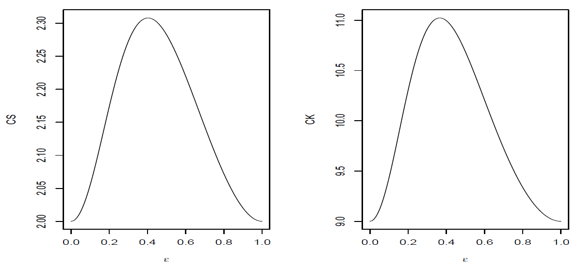
Please note that for any value of , and . It can be seen that and . Figure 3 depicts the behavior of the skewness (CS) and kurtosis (CK) coefficients as a function of . In the figures we observe that the maximum skewness is attained ar , while the maximum kurtosis coefficient is obtained when .
Recall that the survival function of the exponential distribution is of the form and the mean residual life is of the form . Then, it follows from (5), (6) and (9) that if , then the survival and hazard functions and mean residual life are (respectively)
Interestingly, in contrast to the exponential distribution, it can be shown that the hazard function of the EE distribution is not constant, but decreasing in x. This feature can be easily observed in Figure 1 (top panel), where we show the pdf, survival and hazard functions of the EE distribution for different values of the parameter when . Please note that as . Additionally, as .
Suppose and are random variables independently distributed as and , using Theorem 1 the reliability of the system with stress variable () and strength variable () is given by
Please note that when , which corresponds to the stress-strength reliability model of the exponential distributions with parameter for (strength), and with parameter for (stress), respectively.
Maximum likelihood estimations for the parameters and of the epsilon-exponential distribution, can be obtained following the strategy described in Section 2.4 and Section 2.5 (see the Appendix B for details). Let and be random samples from and , respectively. Having estimates of , say , by the invariance property of the MLE, the MLE of R becomes
Numerical Experiments
To illustrate the properties of the estimators we performed a small simulation study considering 5000 simulated datasets for different pair of values of and using Algorithm 1. The goal of the study is to observe the behavior of the MLEs for the model parameters using our proposed EM algorithm considering different sample sizes.
Table 2 summarizes the simulation results. In the table, the columns labeled as “estimate” show the average of the estimators obtained in the simulations, and the columns labeled “SD” show the sample standard deviation of the corresponding estimators. To obtain the standard errors we used the bootstrap method with samples. We observe that the estimates are quite stable and fairly accurate, reporting (on average) numbers close to the true values of the parameters in all cases. Please note that as expected, the precision of the estimates improves as the sample size increase.
4. Survival and Reliability Analysis
Let represent the survival time until the occurrence of a “death” event. In this context, suppose we have n subjects with lifetimes determined by a survival function , and that the ith subject is observed for a time . If the individual dies at time , its contribution to the likelihood function is given by , where is the event density associated with , or equivalently, , where is the corresponding hazard function. On the other hand, if the ith individual is still alive at time and therefore, under non–informative censoring, all we can say is that their lifetime exceeds . It follows that the contribution of a censored observation to the likelihood is simply given by . Notice that in either case we evaluate the survival function at time , because in both cases the ith subject was alive until (at least) time . A death will multiply this contribution by the hazard , but a censored observation will not.
We can combine these contributions into a single expression using a death indicator , taking the value one if individual i died and the value zero otherwise. The resulting likelihood function is of the form
In the next section we will assume that the random variable T follows an epsilon–positive family, and show how estimate the model parameters using the EM algorithm.
4.1. Estimation Using the EM Algorithm
Let denote the survival times, . Using the notation introduced in the previous section, the observed data are a collection of pairs , where the , , are the censoring indicators.
In order implement the EM algorithm, we augment the observed data with the unobservable matrix W defined in Section 2.5, and obtain the (complete) likelihood is given by
with corresponding (complete) log–likelihood .
Then, if be the estimate of at iteration s, and we denote by the conditional expectation of given the observed data and , we obtain
where
Then, for , the iteration s of the algorithm takes the form:
- E–step: For , computewhereand
- M–step: Given and , compute
EM Algorithm for the Epsilon-Exponential Distribution
Suppose that the survival times . Then the EM algorithm takes the form:
- E–step: For , computewhereand
- M–step: Given and , compute
5. Real Data Examples
In this section, we use two examples to illustrate the proposed distributions using (un)censored data sets.
5.1. Example 1: Maintenance Data
First, we consider a real data set originally analyzed by [10]. The complete data set correspond active repair times (in hours) for an airborne communication transceiver, and can be found in Table 3.
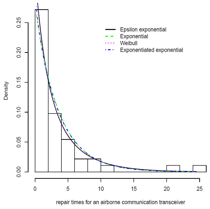
Using the EM algorithm described in Section 4 we fit an epsilon–exponential (EE) distribution to the active repair times. We obtain that the maximized log–likelihood value . Alternatively, we also fit an exponential (Exp), exponentiated–exponential (EExp) and Weibull (Wei) distribution, obtaining the maximized log–likelihood values of , and , respectively. For model comparison, we use the Akaike information criterion (AIC) introduced in [11], given by where is the maximized log–likelihood and k is the number of parameters of the distribution under consideration.
The best model is deemed to be the one with the smallest AIC. For the data set in the example, we obtain , , , and . It follows that in terms of the AIC criteria, the epsilon–exponential shows the best performance when fitting these data. Figure 4 shows the fit of the different models used in the example. Figure 5 displays the three estimated survival functions for this data set.
5.2. Example 2: Recidivism Data
For the second example we use real data obtained from the official records of Gendarmerie of Chile on all inmates released from the Chilean prisons during 2007 after serving a sentence of imprisonment by robbery.
The data set contains records of 9477 inmates and the follow–up period from release until 30 April 2012. In this study, recidivism is defined to occur when a released prisoner goes back to prison for the original or any other offense.
Overall, 52.2% of the inmates in the cohort were convicted of one or more offenses and returned to prison within 64 months of release. About 11.8% of the cohort returned to prison within three months of release, and 30% returned within a year of release.
Table 4 shows the observed proportion of the cohort returning to prison within 1, 3, 6, 12, 18, 24, 36, 48 and 64 months of release. We observe that the cumulative proportion of recidivism grew quickly over the first 12 months after release, increasing by more than 7% every 3 months. After that, the percent increases were smaller and over longer periods.
To analyze the time to recidivism, we determined the number of days between an inmate’s release and his return to prison. Because some inmates did not reoffend, we have censored data and we used the EM algorithm described in Section 4 to fit an epsilon–exponential distribution to the time to recidivism. The maximized log–likelihood value for an assumed epsilon–exponential distribution is easily calculated to be −42,067.84. In comparison, we also fit an exponential distribution yielding a maximized log–likelihood value of −42,632.81.
Looking at the AIC values, we obtain = 84,139.68 and = 85,267.62 for the epsilon–exponential and exponential model respectively, and therefore we conclude, the epsilon–exponential is a better model for these data, based on this criteria.
Finally, we also analyzed the survival time using the Kaplan–Meier estimator. Figure 5 displays the three estimated survival functions for this data set. We observe a close agreement between the Kaplan–Meier survival curve and the epsilon–exponential distribution.
6. Discussion
We introduced a new class of distributions with positive support called epsilon–positive which are generated from any distributions with positive support. This new class of distributions includes the exponential, Weibull, log–normal, etc. ones as special cases. We discussed a stochastic representation for this family, as well as parameter estimation, using the maximum likelihood approach via the Newton–Raphson. In addition, we showed that the elements of this new family can be expressed as a finite scale mixture of positive distributions, which facilitates the implementation of EM-type of algorithms.
We then focused on particular member of this family, called epsilon–exponential distribution, and discuss its applicability in the analysis of survival and reliability data. In this context, we considered the censored data case, and we show how we can use this new family to analyze this type of data sets. For the new class of distributions and, in particular, for the epsilon–exponential distribution we estimate the model parameters using the EM algorithm. An interesting feature of the hazard function of the epsilon–exponential distribution is that is not constant at difference of the exponential one. This feature increases the flexibility of the models allowing its use in a broader range of scenarios.
This greater flexibility is corroborated in the two examples considered in this paper where the AIC criteria shows a better performance our proposed epsilon–exponential model when compared to commonly used alternatives such as the exponential one. The results suggests that the epsilon–exponential distribution should be considered to be a legitimate alternative for the analysis of survival and reliability data in both the censored and uncensored case.
Author Contributions
Conceptualization, R.d.l.C., H.W.G.; methodology, P.C., R.d.l.C., C.F. and H.W.G.; software, P.C.; validation, R.d.l.C. and H.W.G.; formal analysis, P.C.; investigation, P.C., R.d.l.C., C.F. and H.W.G.; resources, R.d.l.C. and H.W.G.; data curation, P.C. and R.d.l.C.; writing–original draft preparation, P.C., R.d.l.C., C.F. and H.W.G.; writing–review and editing, P.C., R.d.l.C., C.F. and H.W.G.; visualization, P.C.; supervision, R.d.l.C. and H.W.G.; project administration, R.d.l.C. and H.W.G.; funding acquisition, R.d.l.C. and H.W.G. All authors have read and agreed to the published version of the manuscript.
Funding
This research was funded by ANID FONDECYT grant number 1181662 & Anillo ACT–87 project, and grant SEMILLERO UA-2021 (Chile).
Institutional Review Board Statement
Not applicable.
Informed Consent Statement
Not applicable.
Data Availability Statement
The data presented in this study are available on request from the corresponding author.
Acknowledgments
The authors would like to thank Gendarmerie of Chile for sharing the data on recidivism used in the paper.
Conflicts of Interest
The authors declare no conflict of interest.
Appendix A. The EE–MLE
For a sample of n independent identically distributed (i.i.d.) observations from , , has to be estimated from the data. The log–likelihood function is given by
Differentiating (A1) with respect to and and equating to 0 respectively, we obtain the likelihood equations
where
and
Please note that no closed form solutions are available to obtain the MLEs of and , respectively. Therefore, the Newton–Raphson algorithm can be implemented. Let and for the epsilon–exponential distribution. Let the vector of first derivatives. Define
The entries , , of the symmetric matrix of second partial derivatives for the epsilon–exponential distribution are
where
and
and the quantities and are defined in Equations (A2) and (A3), respectively.
The functions and define the terms of the Newton–Raphson iteration equation given in (12). To implement the Newton–Raphson algorithm, we can use the moments estimates for and as starting values.
Next, we show that the EM–type algorithm describe in Section 2.5 can be implemented to find the MLEs of the parameters of the epsilon–exponential distribution.
Appendix B. An EM–Type Algorithm for the EE–MLE
In order to implement the EM algorithm to estimate the model parameters of the epsilon–exponential distribution we need to choose in the EM algorithm described in Section 2.5. Let be a random sample from . The complete log–likelihood is
Let be the estimate of at iteration s, and denote by the conditional expectation of given the observed data and . We obtain
where . Therefore, the iteration s of the algorithm takes the form:
- E–step: For , compute
- M–step: Given and , compute
References
- Mudholkar, G.S.; Srivastava, D.K.; Kollia, G.D. A generalization of the weibull distribution with application to the analysis of survival data. J. Am. Stat. Assoc. 1996, 91, 1575–1583. [Google Scholar] [CrossRef]
- Gupta, R.D.; Kundu, D. Exponentiated exponential family: An alternative to gamma and weibull distributions. Biom. J. 2001, 43, 117–130. [Google Scholar] [CrossRef]
- Cooray, K. Analyzing lifetime data with long-tailed skewed distribution: The logistic-sinh family. Stat. Model. 2005, 5, 343–358. [Google Scholar] [CrossRef]
- Fernández, C.; Steel, M.F. On Bayesian modeling of fat tails and skewness. J. Am. Stat. Assoc. 1998, 93, 359–371. [Google Scholar]
- Mudholkar, G.S.; Hutson, A.D. The epsilon skew normal distribution for analyzing near normal data. J. Statist. Plann. Inference 2000, 83, 291–309. [Google Scholar] [CrossRef]
- Arellano-Valle, R.B.; Gómez, H.W.; Quintana, F.A. Statistical inference for a general class of asymmetric distributions. J. Statist. Plann. Inference 2005, 128, 427–443. [Google Scholar] [CrossRef]
- Jones, M. A note on rescalings, reparametrizations and classes of distributions. J. Statist. Plann. Inference 2006, 136, 3730–3733. [Google Scholar] [CrossRef]
- Dempster, A.P.; Laird, N.M.; Rubin, D.B. Maximum likelihood from incomplete data via the em algorithm. J. R. Stat. Soc. Ser. B Stat. Methodol. 1977, 39, 1–38. [Google Scholar]
- Givens, G.H.; Hoeting, J.A. Computational Statistics, 2nd ed.; John Wiley & Sons: New York, NY, USA, 2012. [Google Scholar]
- Chhikara, R.S.; Folks, J.L. The inverse gaussian distribution as a lifetime model. Technometrics 1977, 19, 461–468. [Google Scholar] [CrossRef]
- Akaike, H. A new look at the statistical model identification. IEEE Trans. Automat. Contr. 1974, 19, 716–723. [Google Scholar] [CrossRef]
Figure 1.
Examples of the probability density , survival and hazard functions of epsilon-exponential distribution, , and epsilon-Weibull distribution, . Please note that the exponential and Weibull distributions correspond to the case .
Figure 1.
Examples of the probability density , survival and hazard functions of epsilon-exponential distribution, , and epsilon-Weibull distribution, . Please note that the exponential and Weibull distributions correspond to the case .

Figure 2.
Examples of the probability density , survival and hazard functions of epsilon-log-logistic distribution, , and epsilon-gamma distribution, . Please note that the log-logistic and gamma distributions correspond to the case .
Figure 2.
Examples of the probability density , survival and hazard functions of epsilon-log-logistic distribution, , and epsilon-gamma distribution, . Please note that the log-logistic and gamma distributions correspond to the case .

Figure 3.
Skewness (CS) and kurtosis (CK) coefficientes for .

Figure 4.
The density functions of the fitted epsilon exponential, exponential, Weibull and exponentiated exponential distributions.
Figure 4.
The density functions of the fitted epsilon exponential, exponential, Weibull and exponentiated exponential distributions.

Figure 5.
Fit of the survival functions: Kaplan–Meier estimator (solid line), exponential (dashed line red) and epsilon–exponential (dashed line blue) distributions.
Figure 5.
Fit of the survival functions: Kaplan–Meier estimator (solid line), exponential (dashed line red) and epsilon–exponential (dashed line blue) distributions.


Table 1.
Hazard rate, , Survival, , and density, , functions of some probability models that can be generalized using the definition in (2) In the table .
Table 1.
Hazard rate, , Survival, , and density, , functions of some probability models that can be generalized using the definition in (2) In the table .
| Exponential | |||
| Weibull | |||
| Log-logistic | |||
| Gamma |
Table 2.
Summary of simulation results.
| True Value | n | |||||
|---|---|---|---|---|---|---|
| Estimate | SD | Estimate | SD | |||
| n = 50 | 0.286 | 0.047 | 0.376 | 0.126 | ||
| n = 100 | 0.292 | 0.037 | 0.350 | 0.127 | ||
| 0.3 | n = 200 | 0.292 | 0.030 | 0.335 | 0.118 | |
| n = 500 | 0.295 | 0.022 | 0.317 | 0.106 | ||
| n = 1000 | 0.299 | 0.017 | 0.302 | 0.089 | ||
| n = 50 | 0.287 | 0.054 | 0.558 | 0.133 | ||
| n = 100 | 0.290 | 0.043 | 0.542 | 0.129 | ||
| 0.3 | 0.5 | n = 200 | 0.294 | 0.037 | 0.527 | 0.123 |
| n = 500 | 0.297 | 0.030 | 0.512 | 0.111 | ||
| n = 1000 | 0.298 | 0.023 | 0.506 | 0.091 | ||
| n = 50 | 0.299 | 0.059 | 0.818 | 0.126 | ||
| n = 100 | 0.299 | 0.047 | 0.809 | 0.122 | ||
| 0.8 | n = 200 | 0.301 | 0.038 | 0.801 | 0.108 | |
| n = 500 | 0.303 | 0.029 | 0.794 | 0.088 | ||
| n = 1000 | 0.302 | 0.022 | 0.794 | 0.069 | ||
| n = 50 | 0.476 | 0.079 | 0.379 | 0.125 | ||
| n = 100 | 0.484 | 0.062 | 0.355 | 0.125 | ||
| 0.3 | n = 200 | 0.486 | 0.049 | 0.337 | 0.121 | |
| n = 500 | 0.494 | 0.037 | 0.316 | 0.107 | ||
| n = 1000 | 0.497 | 0.029 | 0.303 | 0.088 | ||
| n = 50 | 0.477 | 0.088 | 0.558 | 0.133 | ||
| n = 100 | 0.484 | 0.074 | 0.542 | 0.131 | ||
| 0.5 | 0.5 | n = 200 | 0.488 | 0.059 | 0.528 | 0.124 |
| n = 500 | 0.494 | 0.048 | 0.512 | 0.109 | ||
| n = 1000 | 0.498 | 0.039 | 0.502 | 0.091 | ||
| n = 50 | 0.484 | 0.104 | 0.838 | 0.129 | ||
| n = 100 | 0.499 | 0.076 | 0.809 | 0.119 | ||
| 0.8 | n = 200 | 0.503 | 0.064 | 0.799 | 0.110 | |
| n = 500 | 0.505 | 0.049 | 0.793 | 0.089 | ||
| n = 1000 | 0.504 | 0.038 | 0.793 | 0.070 | ||
| n = 50 | 0.762 | 0.125 | 0.374 | 0.124 | ||
| n = 100 | 0.771 | 0.099 | 0.356 | 0.125 | ||
| 0.3 | n = 200 | 0.779 | 0.080 | 0.336 | 0.120 | |
| n = 500 | 0.789 | 0.058 | 0.314 | 0.105 | ||
| n = 1000 | 0.796 | 0.046 | 0.301 | 0.089 | ||
| n = 50 | 0.765 | 0.139 | 0.555 | 0.134 | ||
| n = 100 | 0.771 | 0.116 | 0.543 | 0.134 | ||
| 0.8 | 0.5 | n = 200 | 0.782 | 0.096 | 0.528 | 0.123 |
| n = 500 | 0.789 | 0.076 | 0.515 | 0.110 | ||
| n = 1000 | 0.797 | 0.062 | 0.503 | 0.091 | ||
| n = 50 | 0.791 | 0.153 | 0.815 | 0.130 | ||
| n = 100 | 0.800 | 0.126 | 0.804 | 0.122 | ||
| 0.8 | n = 200 | 0.798 | 0.103 | 0.798 | 0.106 | |
| n = 500 | 0.806 | 0.079 | 0.794 | 0.089 | ||
| n = 1000 | 0.807 | 0.060 | 0.793 | 0.070 | ||
Table 3.
Repair times (in hours) of 46 transceivers.
| 0.2 | 0.3 | 0.5 | 0.5 | 0.5 | 0.5 | 0.6 | 0.6 | 0.7 | 0.7 |
| 0.7 | 0.8 | 0.8 | 1.0 | 1.0 | 1.0 | 1.0 | 1.1 | 1.3 | 1.5 |
| 1.5 | 1.5 | 1.5 | 2.0 | 2.0 | 2.2 | 2.5 | 2.7 | 3.0 | 3.0 |
| 3.3 | 3.3 | 4.0 | 4.0 | 4.5 | 4.7 | 5.0 | 5.4 | 5.4 | 7.0 |
| 7.5 | 8.8 | 9.0 | 10.3 | 22.0 | 24.5 |
Table 4.
Observed recidivism by time after release.
| Time after Release | % Observed Recidivists |
|---|---|
| 1 month | 4.7% |
| 3 month | 11.8% |
| 6 month | 19.9% |
| 12 month | 30.0% |
| 18 month | 35.9% |
| 24 month | 40.8% |
| 36 month | 46.6% |
| 48 month | 50.4% |
| 64 month | 52.2% |
Publisher’s Note: MDPI stays neutral with regard to jurisdictional claims in published maps and institutional affiliations. |
© 2021 by the authors. Licensee MDPI, Basel, Switzerland. This article is an open access article distributed under the terms and conditions of the Creative Commons Attribution (CC BY) license (https://creativecommons.org/licenses/by/4.0/).
Share and Cite
MDPI and ACS Style
Celis, P.; de la Cruz, R.; Fuentes, C.; Gómez, H.W. Survival and Reliability Analysis with an Epsilon-Positive Family of Distributions with Applications. Symmetry 2021, 13, 908. https://0-doi-org.brum.beds.ac.uk/10.3390/sym13050908
AMA Style
Celis P, de la Cruz R, Fuentes C, Gómez HW. Survival and Reliability Analysis with an Epsilon-Positive Family of Distributions with Applications. Symmetry. 2021; 13(5):908. https://0-doi-org.brum.beds.ac.uk/10.3390/sym13050908
Chicago/Turabian StyleCelis, Perla, Rolando de la Cruz, Claudio Fuentes, and Héctor W. Gómez. 2021. "Survival and Reliability Analysis with an Epsilon-Positive Family of Distributions with Applications" Symmetry 13, no. 5: 908. https://0-doi-org.brum.beds.ac.uk/10.3390/sym13050908
Note that from the first issue of 2016, this journal uses article numbers instead of page numbers. See further details here.