Numerical Investigation of Mixing by Induced Electrokinetic Flow in T-Micromixer with Conductive Curved Arc Plate

Abstract

Mixing is essential in microdevices. Therefore, increasing the mixing efficiency has a significant influence on these devices. Using conductive obstacles with special geometry can improve the mixing quality of the micromixers. In this paper, a numerical study on the mixing caused by an induced-charge electrokinetic micromixer was carried out using a conductive plate with a curved arc shape instead of a conductive flat plate or other non-conductive obstacles for Newtonian fluids. This study also explored the effect of the different radius curves, span length, the number of curved arc plates in the channel, the pattern of arrangement, concavity direction, and the orientation angle against the flow on the mixing. Furthermore, the efficiency of the T-micromixer against a flow with a low diffusion coefficient was investigated. It should be noted that the considered channel is symmetric regarding to the middle horizontal plane and an addition of flat plate reflects a formation of symmetric flow structures that do not allow to improve the mixture process. While an addition of non-symmetric curved arc plates al-lows to increase the mixing by creating vortices. These vortices were created owing to the non-uniform distribution of induced zeta potential on the curved arc plate. A rise in the span length of the curved arc plate when the radius was constant improved the mixing. When three arc plates in one concavity direction were used, the mixing efficiency was 91.86%, and with a change in the concavity direction, the mixing efficiency increased to 95.44%. With a change in the orientation angle from 0 to 25, the mixing efficiency increased by 19.2%.

1. Introduction

The development and application of microfluidic equipment in industries such as pharmacy, chemistry, and the laboratory have attracted the attention of researchers. Thus far, various phenomena in microwave equipment have been investigated by researchers. The mixing process is one of these phenomena. Mixing in micro-dimensions is very important due to its application in biochemistry, drug delivery, Lab-on-Chip, and bacterial detection [1,2,3,4]. A rapid mixing process is not achieved easily to create a homogeneous solution at a small scale (micro) in the chemical and medicinal industries. Weak mixing creates a heterogeneous mixture that affects the accuracy of outcomes. The mixing process of two or more fluids in microchannels, without applying micromixers or employing mechanical micromixers and according to the laminar flow regime, entirely depends on molecular diffusion in these channels. Therefore, the most significant limitation in microchannels is the impossibility of generating a flow with high disturbances. As a result, this slows down the mixing process. On a micro-scale, the use of conventional techniques usually requires moving parts because manufacture and assembly on this scale are complicated. If the contact surface of the two fluids is small and the circulation strength is great, long microchannels and much time are needed to achieve acceptable mixing.

Generally, micromixers include two categories, namely active and passive. In passive mixers, mixing is performed because of the mixer’s particular geometry, changing the direction of the fluid, and without the involvement of external factors such as fluid lamination, intersection or twisting of the fluid, or by creating obstacles [5]. In contrast, in the active mixers, an external factor or moving parts cause the mixing of fluids [6]. The external factor can be energy, which can be supplied by various methods, such as an electric field, magnetic field, thermal field, electrophoresis, ultrasonic vibration, or by using an oscillating input in the microchannels.

The application of an electric field as an active technique is employed to increase and improve the mixing phenomenon. One of the most important and effective methods in micromixers is the use of electrokinetic phenomena. In the flows where the pressure difference between upstream and downstream is the agent of fluid flow, the basic assumption of fluid mechanics is to consider zero velocity on a solid surface (the principle of non-slipping). As a result of this type of flow (for example, the laminar flow), a parabolic velocity profile is created. However, in the electrokinetic phenomenon, the agent of the liquid flow is the application of an external electric influence. The electrokinetic phenomenon is characterized by the coupling of the applied electric influence with an electric charge layer on the solid surface in contact with the electrolyte solution within the microchannel. The thin layer of the electric charges formed in a solution along the microchannel wall is referred to as an electric double layer. By applying an external electric field on this layer, an electrokinetic phenomenon is created.

Squires et al. [7] and Bazant et al. [8], for the first time, examined the theory and applications of electrokinetic phenomena in microfluidics. They introduced the electrokinetic flow of induced-charge electroosmosis (ICEO) and considered the usage of an electroosmosis AC current around metal microstructures to produce eddies for a microfluidic mixture. The most important feature of ICEO is the creation of fluid motion near the conductive body under the external electric influence. The reason for this is the induced non-uniform load on solid and fluid interfaces. This circulating flow causes better mixing in the microchannel.

Wu et al. [9] presented a numerical method that correctly simulates electrokinetic flow on conducting surfaces. The accuracy of the numerical method presented by them is investigated by the analytic relation of Squires and Bazant [7].

Wu and Li [9,10] simulated the conductive electric hurdles in the induced-charge electroosmosis flow and compared them with experimental results. Their simulations showed that when vortices were produced close to the hurdles, the mixing of the components could be significantly increased. By placing the conductive hurdles in the applied electric field, the distribution of the zeta potential on the conductive surfaces will be non-uniform. As a result, by changing the position, the electroosmosis motion velocity on the conductive sheets changes, and a non-uniform circulation pattern is created.

The most important feature of the circulation pattern, as Wu and Li showed, is that eddies are produced close to the solid blocks. Circulation of the liquid close to these solid blocks is created owing to sheets with opposite zeta potentials. A different sign of the induced zeta potential indicates the opposing electroosmosis motion driving forces, which reflect the circulation of the liquid [7,9]. Their results have shown that increasing the mixing is dependent on the geometry of the hurdles. Rectangular hurdles also have the best effect on increasing mixing. With the addition of the conductive hurdles in series, the vortices increase and then cause an increase in the mixing.

Wu et al. [11] demonstrated a theoretical approach for the mixing process caused by diffusion phenomena. The dimensionless analysis provided by them is suitable for use in microchannels with different sizes and different diffusion coefficients. They also examined the analytical model by manufacturing simple microchannels.

Daghighi et al. [12,13] performed numerical and experimental work on the electroforce motion of conductive particles. The proposed micromixer in their work was started by a battery (DC field). They observed that some regions of the returning and circulating flow were formed around a non-electric conductive surface. Shamloo et al. [14] considered three geometries containing a single ring, diamond, and two rings for electroosmosis mixers, and through numerical calculations, they obtained a mixing coefficient above 98%. Shamloo et al. [15] used different numbers and geometries of conductive hurdles in an electroosmosis micromixer. The geometry of hurdles was square, triangle, and circle. They studied the influence of the scale and numbers of the geometries on the mixing time and efficacy. The best result was obtained for the triangular mixing chamber with circular hurdles. They concluded that the use of two circular conductive hurdles is a useful way to enhance the mixing parameter and reduce the mixing time.

Azimi et al. [6] used a flexible conductive rod connected to the microchannel wall and scrutinized the influence of the number of these rods, the parallel and opposite arrangements, and the distance between them on the fluid physics. Azimi et al. [16] employed a flexible conductive flap within a micromixer inside a DC field, to create rapid mixing and vortices. They revealed that a sheet with a low Young’s modulus had a large mixing zone and improved the mixing process. Alipanah et al. [17] performed numerical studies of a micromixer with alternating electric induction. They investigated the mixing efficiency with numerical simulation of a T-micromixer and concluded that with alternating electroosmosis induction, the mixing length decreases, and mixing efficiency increases.

Cetkin and Miguel [18] modeled three types of passive branch micromixers numerically and calculated mixing efficacy and flow impedance using the computational outcomes for all models. An optimum design is presented in terms of minimum flow impedance and the best mixing efficiency. Khozeymeh-Nezhad [19] and Niazmand simulated an active micromixer with an oscillating stirrer and, by using non-dimensional parameters, presented an optimum model in terms of mixing efficiency.

Bhattacharyya et al. [20] studied the numerical electroosmosis flow in micromixers with a rough surface. Roughness, as a rectangular hurdle, was created on the micromixer. They found that the circulations were created on the upper part of the hurdle. These circulating flows increased the mixing rate in the micromixer. Cho et al. [21,22] analyzed the enhancement of mixing in cross-over micromixers using an unstable electroosmosis turbulent flow. They found that periodic electric potentials could lead to erratic and occasional vortices within the lateral channels. These vortices encounter the flow in the major channel and lead to mixing for two circulations. Accordingly, the contact interface and the mixing index increase.

Peng and Li [23] scrutinized the effect of the ionic concentration in the electroosmotic mixing of two fluids with different concentrations and developed a mathematical model for this process. They studied the dependency of the zeta potential, dielectric constant, and electric conductivity on the concentration. They showed that the electroosmosis method does not adequately mix a mixture with a high ionic concentration and with a low-concentration solution. Nazari et al. [24] presented a mixer with a new mixing chamber and obtained the optimal model by changing the position of the conductive blocks and the shape of the cavity. They used four geometries for the mixing chamber, including square, rhomboid, triangular, and circular. The authors investigated the stream fields and mixing efficiency by changing the conductive surfaces in each geometry. They showed that a rhomboid-shaped mixing conductive chamber with 95% mixing efficiency had the highest efficiency in comparison with the other geometries. Nazari et al. [25] conducted a complete computational analysis and geometric analysis on the effect of the micromixer’s conductive surface. They used the simple plate as a conductive hurdle and studied the impact of the angle, position, length, and number of the plates on the efficacy, velocity field, and streamlines. The highest efficiency was achieved for the case in which three plates with a 5-degree angle were used. Deng et al. [26] presented an optimum model of the position of electrode pairs in an electroosmotic micromixer. They presented their results numerically. Chen et al. [27] investigated micromixers with serpentine channels using experimental and numerical approaches. They studied mixing efficiency in terms of a Reynolds number between 0.1 and 100, and they observed that the mixing efficiency increased for a Reynolds number from 0.1 to 1 and decreased from 1 to 100.

Hadigol et al. [28] performed a numerical analysis for non-Newtonian (power-law) fluid in a combined pressure and electroosmotic flow. The microchannel geometry was considered as a simple rectangular channel, and the effects of the n-zeta potential index and EDL thickness on the electroosmotic flow and the composition of the osmotic compressive flow were investigated. They found that by increasing the zeta potential at n < 1, an increased flow rate and pressure rise in the electroosmotic flow were observed. However, these changes for n > 1 would not have a significant effect on the flow rate and pressure rise.

Choi et al. [29] conducted a numerical study on power-law non-Newtonian fluid for a fully developed flow within a rectangular microchannel. They studied the effect of change in zeta potential on different parts of the microchannel walls. The effect of different fluid behavior indexes, different aspect ratios, and electrochemical properties on the velocity profile and flow rate within the microchannel was studied and presented.

Tatlιsoz and Canpolat [30] performed a numerical simulation for pulsatile flow micromixing with electroosmotic flow for Newtonian and non-Newtonian fluids. They also selected blood-like properties for non-Newtonian fluids. For non-Newtonian fluids, they investigated power-law and Carreau models for the effect of n on flow behavior and mixing efficiency. They found that the combination of pulsatile flow and electroosmotic flow for the Newtonian fluid dramatically increased the mixing efficiency, and a fully mixed mixture could be achieved in 10 s.

Abdelmalek and Abdollahzadeh Jamalabadi [31] performed numerical simulations of a micromixer with a moving cylinder inside the channel. A parametric study was performed on the amplitude and frequency of the moving cylinder in mixing the fluid. Their results showed a significant increase in mixing efficiency due to the presence of the moving cylinder within the channel. Using computational fluid dynamics, Karvelas et al. [32] simulated a micromixer for mixing water and iron oxide nanoparticles. Different inlet velocities and inlet angles of the two streams were studied, and their effect on mixing was investigated. They concluded that the angles between two inputs play little role in mixing.

Liosis et al. [33] conducted a numerical study on the mixing of magnetic particles in contaminated water under an external magnetic field in a rectangular microchannel. Their results showed that by decreasing the frequency and increasing the amplitude of the magnetic field, the mixing efficiency increases, and a better distribution of particles within the channel can be achieved. Wu and Lai [34] conducted a numerical study on a T-shaped micromixer with a vortex generator obstacle at the input. They studied the effect of geometric variables such as obstacle distance and obstacle angle on micromixer performance. The results showed that mixing increased with an increasing Reynolds number.

The literature review shows that different obstacles play a vital role in the mixing efficiency of a micromixer. Moreover, the presence of conductive or non-conductive obstacles could affect the quality of the mixing. In the literature review, the effect of the different non-conductive obstacles, such as plate, circle, rectangle, and rhomboid, on the mixing quality has been investigated. Some literature works have highlighted the impact of a conductive plate and conductive elastic plate on mixing quality. However, the impact of geometrical variation in the shape of a conductive mixing plate has not been well addressed. The present study aims to address the impact of the geometrical design of a conductive arc shape mixing plate on the mixing behavior of a micromixer. The influence of zeta potential on the vortex phenomenon around the curved plate is discussed.

2. Governing Equations

In the present study, the equations of the electrodynamic, hydrodynamic, and mass transport for the geometry of a micromixer have been coupled and solved. The governing mathematical equations are further explained.

2.1. Electrodynamic

By using an electric influence and solving the Laplace equation (Equation (1)), the applied electric potential of the electrolyte fluid can be calculated as follows [16]:

$${\nabla }^2{\overline{\varphi }}_e=0$$

(1)

The conductive surfaces are considered to be completely conductive, so a stable electric double layer is formed on the sheets. Therefore, it prevents the passage of electric flow from conductive surfaces. For this reason, we can consider the boundary condition of the Laplace equation as insulators on the conducting surfaces. The Laplace equation is calculated with the following boundary restrictions:

$$\overline{n}\nabla {\overline{\varphi }}_e=0\mathrm{on}\mathrm{the}\mathrm{walls}\mathrm{of}\mathrm{the}\mathrm{microchannel}\mathrm{and}\mathrm{conductive}\mathrm{surfaces}$$

(2)

$${\overline{\varphi }}_e={\varphi }_0\mathrm{the}\mathrm{inlet}\mathrm{of}\mathrm{the}\mathrm{microchannel}$$

(3)

$${\overline{\varphi }}_e=0\mathrm{the}\mathrm{outlet}\mathrm{of}\mathrm{the}\mathrm{microchannel}$$

(4)

2.2. Flow Equations

Assuming the incompressible and Newtonian fluid, the flow field can be solved by using the continuity equation [6]:

$$\nabla \overline{u}=0$$

(5)

and Navier–Stokes equation:

$$\rho \left(\frac{\partial \overline{u}}{\partial t}+\left(\overline{u}\nabla \right)\overline{u}\right)=-\nabla P+\mu {\nabla }^2\overline{u}$$

(6)

In these equations, ρ is the liquid density, $\nabla P$ is the pressure gradient, μ is the liquid viscosity, and $\overline{u}$ is the liquid velocity. Given that the nature of the problem is transient, term $\partial \overline{u}/\partial t$ should not be deleted. The boundary restrictions for solving the circulation patterns are as follows:

$$\overline{u}=\frac{-\epsilon {\epsilon }_0{\zeta }_w}{\mu }\overline{E}\mathrm{on}\mathrm{the}\mathrm{micromixer}\mathrm{walls}$$

(7)

$$\overline{u}=\frac{-\epsilon {\epsilon }_0{\zeta }_i}{\mu }\overline{E}\mathrm{on}\mathrm{the}\mathrm{conductive}\mathrm{surfaces}$$

(8)

$$\overline{n}\nabla \overline{u}=0\mathrm{inlet}\mathrm{and}\mathrm{outlet}$$

(9)

Here, $\overline{E}=\nabla {\overline{\varphi }}_e$ is the locally applied electric field. It should be noted that in the non-conductive microchannel wall, the value of ζ_w is constant. However, in the conducting surfaces, it is induced, and it is equal to ζ_i. When the inside of the microchannel is filled with an electrolyte, an electric double layer is formed near the solid surfaces [8]. The boundary between the EDL layers is called the shear plate and the electrical potential at this boundary is called the zeta potential. Zeta potential is the approximate size of the surface potential in electrokinetic models. In classical electrokinetics, this value is constant.

In the present electroosmotic flow, flow is caused by the electric field. Therefore, there is no pressure difference between the inlet and outlet. It can be stated that the pressure boundary condition on the inlet and outlet of the channel is as follows:

$$P=0\mathrm{at}\mathrm{the}\mathrm{inlets}\mathrm{and}\mathrm{outlet}$$

(10)

$$\overline{n}\nabla P=0\mathrm{on}\mathrm{the}\mathrm{microchannel}\mathrm{walls}$$

(11)

2.3. Concentration Field

Assuming that no reaction occurs in the electroosmotic flow, the concentration field of the electrolyte solution is as follows:

$$\frac{\partial C}{\partial t}+\overline{u}\nabla C=D{\nabla }^{2}C$$

(12)

Here, C is the local concentration, and D is the diffusion parameter. The diffusion coefficient D in most of the electrolyte solutions has an approximate value of 10⁻¹⁰ m²/s. In this case, it is assumed that the walls are impermeable. The boundary conditions for Equation (12) are given below:

C = C₀, concentration in the inlet 1

(13)

C = 0, concentration in the inlet 2

(14)

C = 0, concentration in the outlet for time t = 0

(15)

$${\frac{\partial C}{\partial n}|}_{t\ge 0}=0,\mathrm{concentration}\mathrm{gradient}\mathrm{at}\mathrm{all}\mathrm{flux}\mathrm{micromixer}\mathrm{walls}$$

(16)

3. Geometry, Computational Domain, and Validation

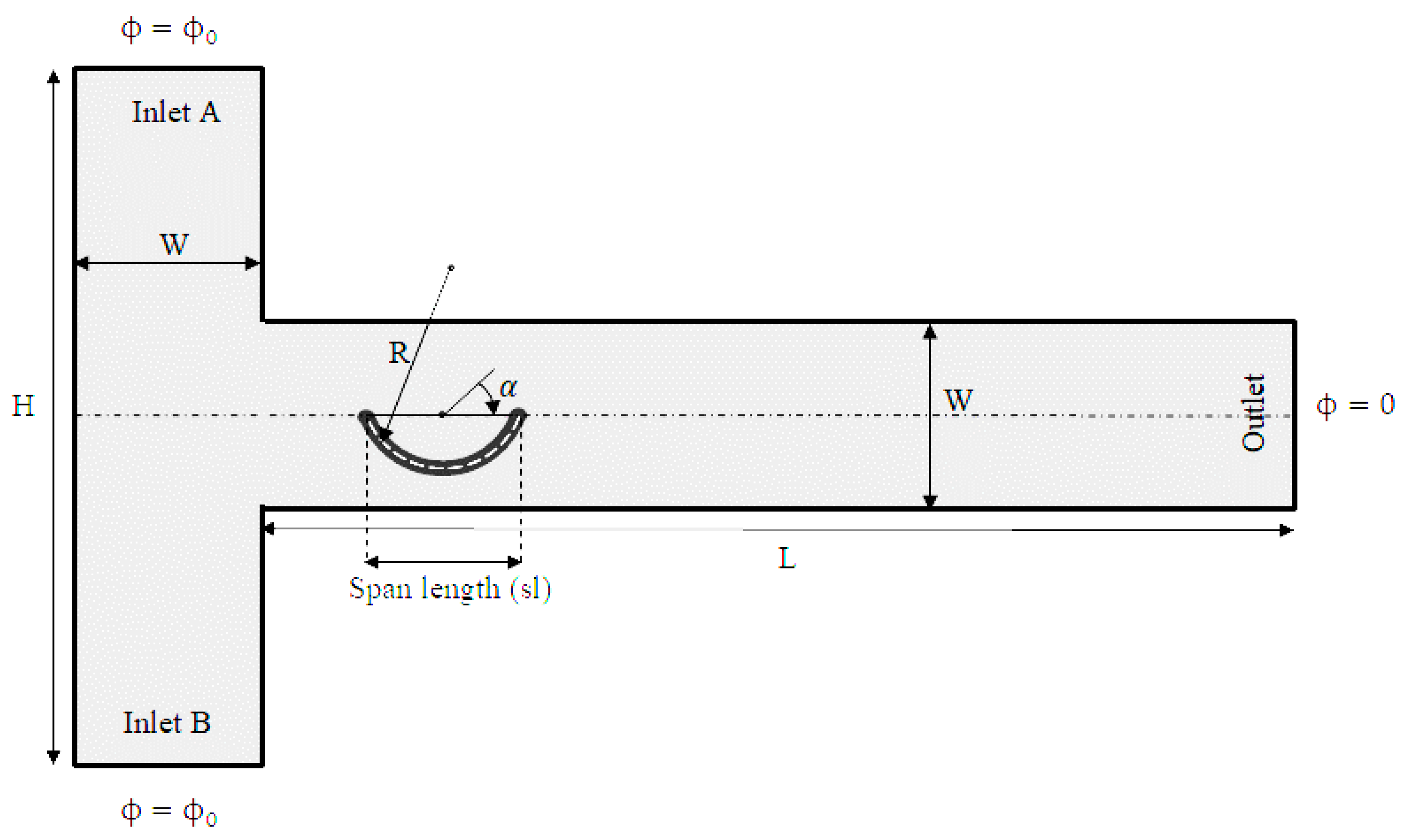
In the present study, a T-micromixer is investigated, which contains two inlets, one outlet, and a conductive curved arc plate as hurdles, and the length of the vertical inlet channel and the length of the horizontal channel is H = 5 W and L = 10 W, respectively, where W is the width of the two channels. The thickness of the arc is 0.1 W. It should be noted that the considered channel is symmetric regarding the middle hor-izontal plane and an addition of flat plate along this middle plane can reflect a for-mation of symmetric flow structures. The inlet of the microchannel is on the left side and has two fluid flows with different concentrations. In inlet A, fluid with a concentration of C₁ = 1 enters the micromixer, and in inlet B, fluid with a concentration of C₂ = 0 enters the micromixer. Electrodes are located at both ends of the channel to create an electric field and fluid drift that is modeled with two electric potential difference boundary conditions. Microchannel walls and the surfaces of the curved arc plate are considered electrically insulated. The pressure gradient between the inlet and outlet of the channel is considered zero. Zeta potential is considered on the wall equal to −0.05 V. Other fluid specifications are provided in

Table 1. Fluid and geometry specifications.

Values	Symbol	Parameters
100	W (μm)	Width of the channel
0.7 W	R (μm)	Radius
500	H (μm)	Length of the vertical channel
1000	L (μm)	Length of the horizontal channel
1 W	sl (μm)	Span length
0.1 W	t (μm)	Thickness
1000	ρ (kg/m3)	Fluid density
0.001	μ (Pa/s)	Viscosity
80	ε	Dielectric constant
−0.05	ζw (V)	Zeta potential on the wall
1	C1 (mol/m3)	Inlet concentration at entrance A
0	C2 (mol/m3)	Inlet concentration at entrance B
100	(V/cm)	Horizontal electric field

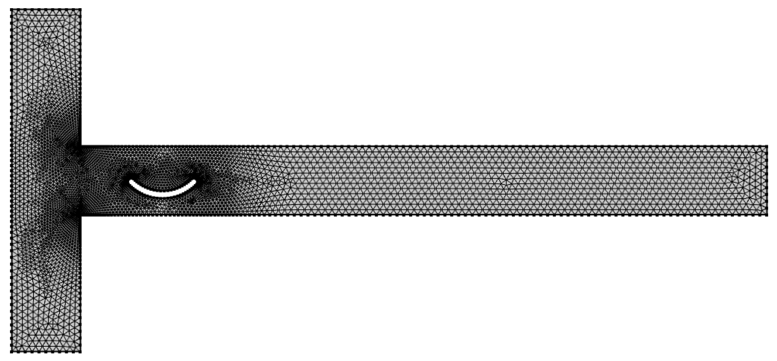
. Figure 1 shows the geometry of the T-micromixer with an arc plate, and Figure 2 shows the computational domain with triangular meshes. The computational grid becomes smaller due to the increased number of flow changes around the conductive curved arc plate.

Squires and Bazant’s [8] equation to obtain an induced zeta potential on the surface of a 2D cylinder is presented as Equation (17):

$${\zeta }_i\left(\theta \right)=\overline{E}d\cdot \cos \left(\theta \right)$$

(17)

Here, θ is the angular coordinates, and d is a cylinder radius. This equation is not accurate for irregular shapes or complex geometry and is only useful for simple and regular geometries. No simple analytical solution is available for induced zeta potential at conductive surfaces with irregular shapes or complex geometry. Numerical methods can eliminate this limitation. In this paper, the numerical method presented by Wu and Li is used to calculate induced zeta potential. In this method, the distribution of zeta is as follows:

$${\zeta }_{\mathrm{induced}}=-{\varphi }_e+{\varphi }_c$$

(18)

In this equation, φ_e is the external electric potential, and φ_c is the constant correction potential on the surface of the conductive body. If the surface of the body is initially considered without charge, then the integration of the induced charges on the surface of the conductive body should be zero:

$${\displaystyle \underset{S}{\oint }{\zeta }_{\mathrm{induced}}}dS=0$$

(19)

If integration with Equation (18) is done, the following equation is obtained according to Equation (19):

$${\varphi }_c=\frac{{\displaystyle \underset{S}{\oint }{\varphi }_e}dS}{S}$$

(20)

Therefore, for calculating the induced zeta potential ${\zeta }_i$, the following equation is used:

$${\zeta }_i=-{\varphi }_e+\frac{{\displaystyle \underset{S}{\oint }{\varphi }_e}dS}{S}$$

(21)

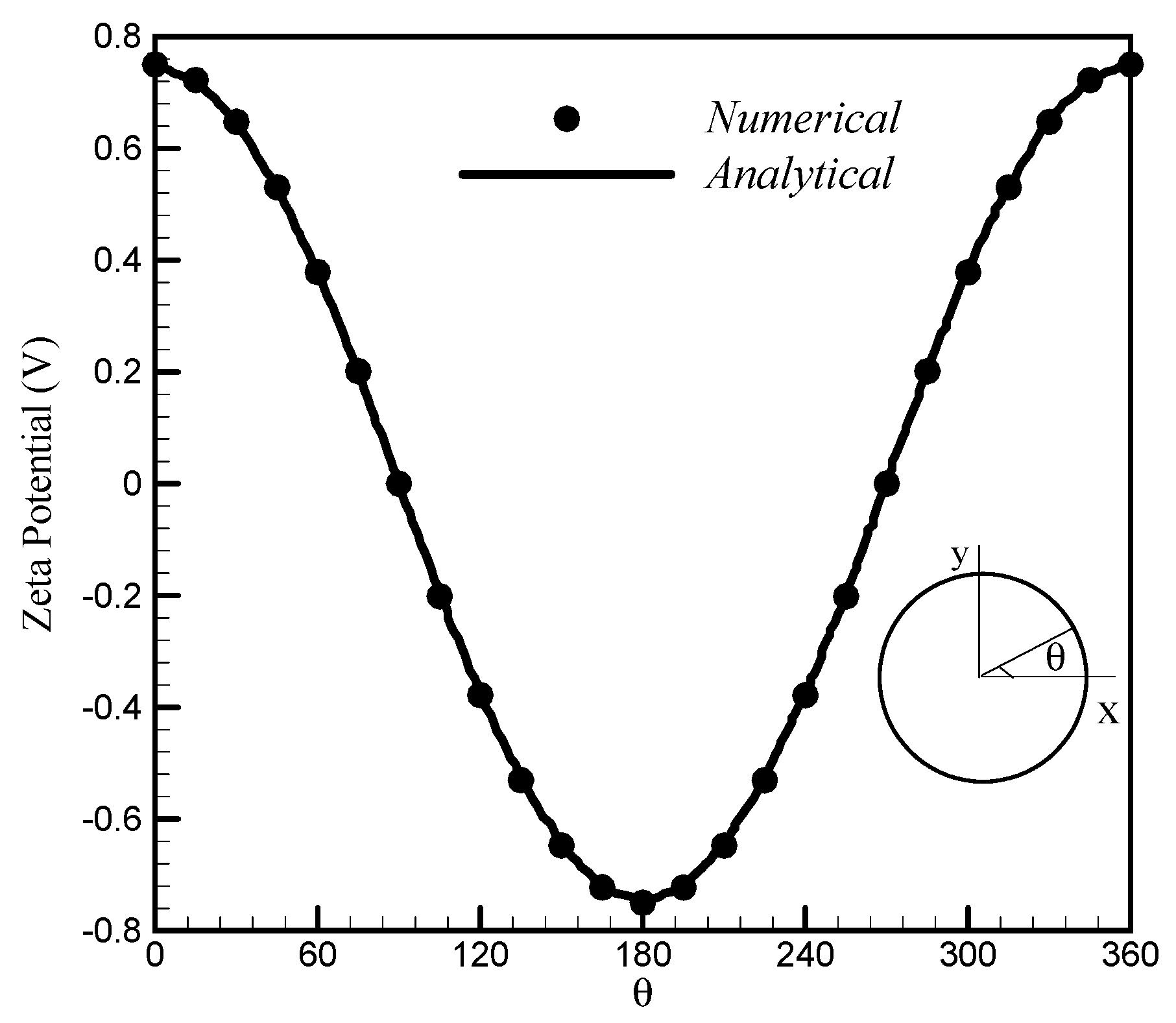
The numerical and analytical results for induced zeta potential are shown in Figure 3. A cylinder with a diameter of d = 30 μm is considered under an electric field of 250 V/cm. As shown in Figure 3, the numerical results have high accuracy and a minor difference from the analytical calculations.

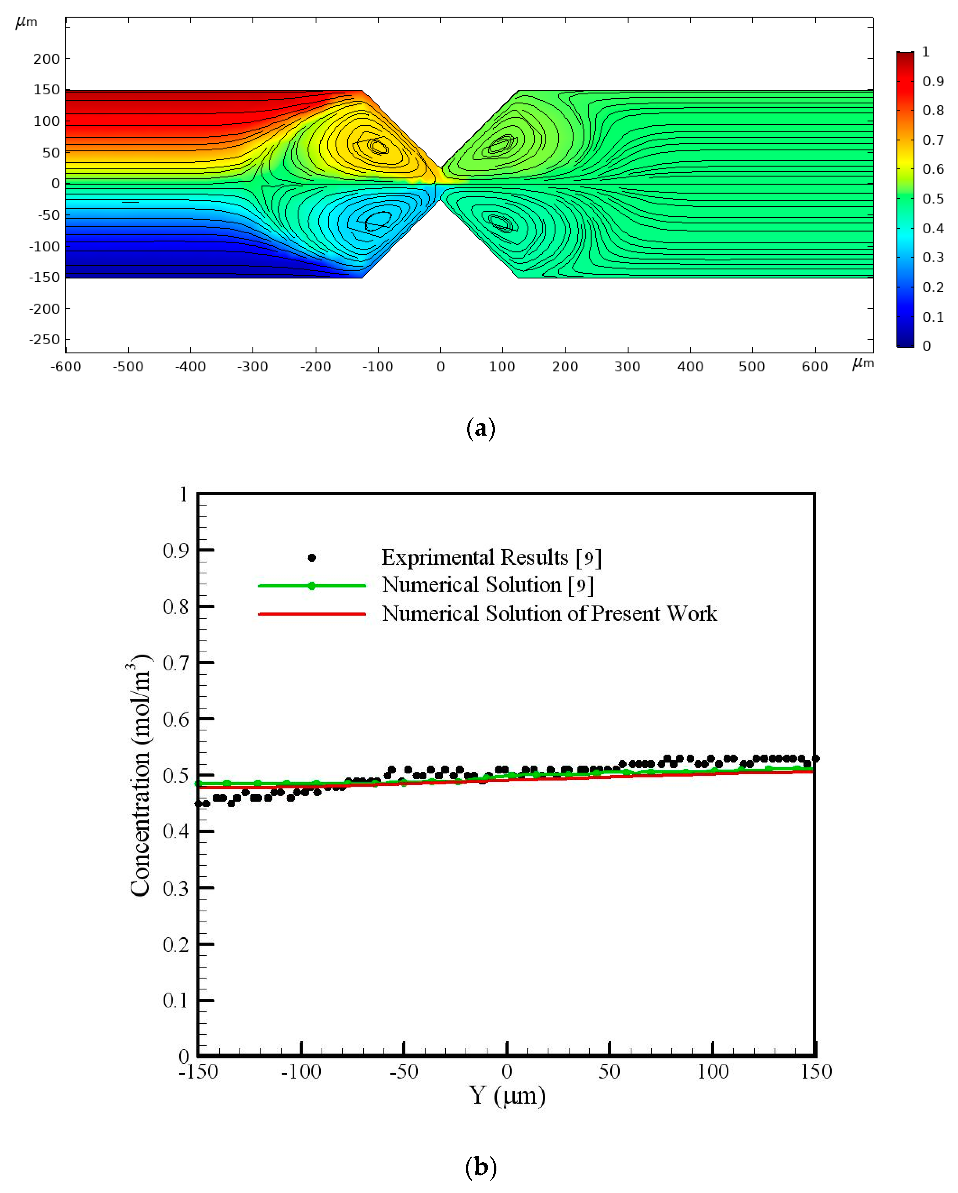
The validation of the results is performed with the experimental outcomes of Wu and Li. In Figure 4, the comparison of the numerical results of the present study with experimental and numerical results of Wu and Li’s paper [9] is shown. Wu and Li used two symmetrical triangular conductor hurdles [9]. In Figure 4a, the concentration counter and streamlines near the triangular hurdles are shown. The rotational flow created around these hurdles, which increases mixing, is quite apparent. In Figure 4b, the concentration distribution in the cross-section at a distance of 2000 μm from the hurdles is shown to indicate the acceptable accuracy of the numerical solution.

COMSOL Multiphysics^® version 5.4 is used for simulating and creating the computational grid. The Navier–Stokes equations and the concentration equation are coupled through the velocity field and solved transient. A relation is entered to calculate the induced zeta potential (Equation (21)) and its relation to the velocity (Equation (8)) entered into the calculations. The time used to reach a steady electric field is very short compared to the time of the other processes such as diffusion and transfer [8]. For this reason, in the numerical solution, a steady electric field is assumed.

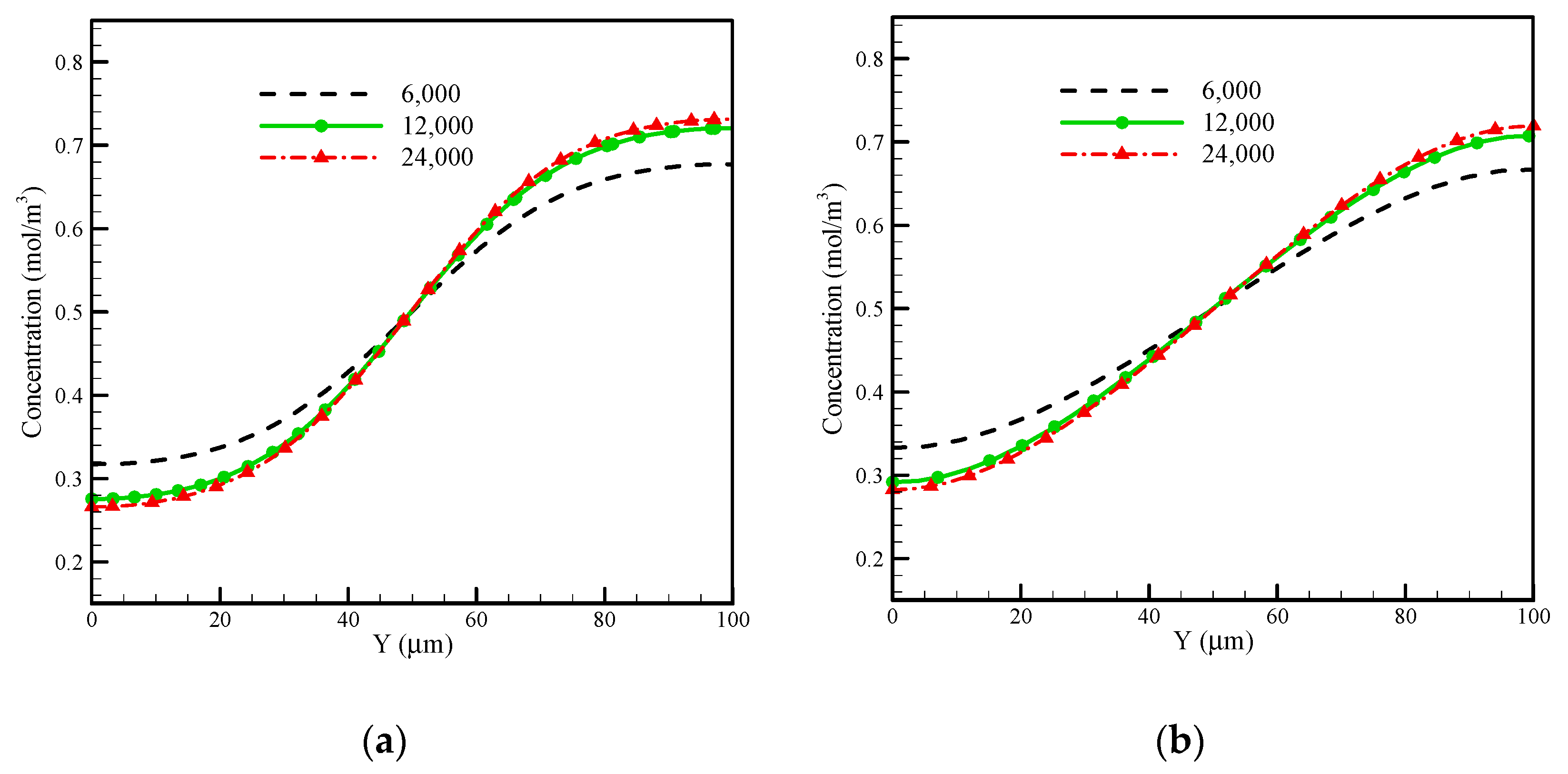
Due to the importance of the non-dependence of numerical solution results on the computational grid, the results are compared for the grids with different values of computational elements, and independence of the outcomes from the computational grid is investigated for the present model. Generally, with an increasing number of cells in the computational grid, the accuracy of the numerical solution as well as the computational cost increases. Thus, using a fair grid with acceptable accuracy and reasonable computational cost is essential. For investigating the independence of the solution from the grid, three grids with 6000, 12,000, and 24,000 elements were tested. The concentration distribution of these grids is shown in Figure 5. According to Figure 5, the difference between grids with 12,000 and 24,000 elements can be ignored. Therefore, the computational grid with 12,000 elements was adopted.

4. Results and Discussion

The results of the present work have a lower mixing time and mixing length compared to the results of other studies that used passive T-shape micromixers. Moreover, the geometry used in the present work is clearly simpler [35,36]. In this section, the computational outcomes, obtained for improving the performance of the micromixer, are presented. First, the effect of the arc curve on the flow field, concentration distribution, and mixing efficacy is investigated. Then, the effect of the radius, span size, angle of the position, number and position of the arc curve, and the diffusion coefficient is studied.

Equation (22) was used to define the mixing efficacy in an induced electrokinetic mixer. In this regard, C_∞ = 0.5 is the best mixing rate on a normal scale. C₀ is the concentration at the channel inlet, and C is the concentration at the desired cross-section downstream of the flow [9]. Clearly, in full mixing conditions, the efficiency will be 100%.

$$\epsilon =\left(1-\frac{{\displaystyle \underset{0}{\overset{W}{\int }}\left|C-C_{\infty }\right|}dx}{{\displaystyle \underset{0}{\overset{W}{\int }}\left|C_0-C_{\infty }\right|}dx}\right)\times 100$$

(22)

In the presence of conductive hurdles, the shape of the flow changes considerably. In the vicinity of the hurdles, there are vortices that cause further mixing. The induced zeta potential on the conductive body has opposite signs, which causes the circulation of the flow. In the electric double layer, in places where the zeta potential is positive, there is a negative charge that creates a motion to the inlet of the microchannel. Instead, in zones with negative zeta potential, a positive charge is formed in the electric double layer, which creates a fluid flow to the outlet of the channel. As a result, rotation will occur to satisfy the flow continuity condition, followed by an increase in mixing.

4.1. The Effect of the Presence of an Arc Curve

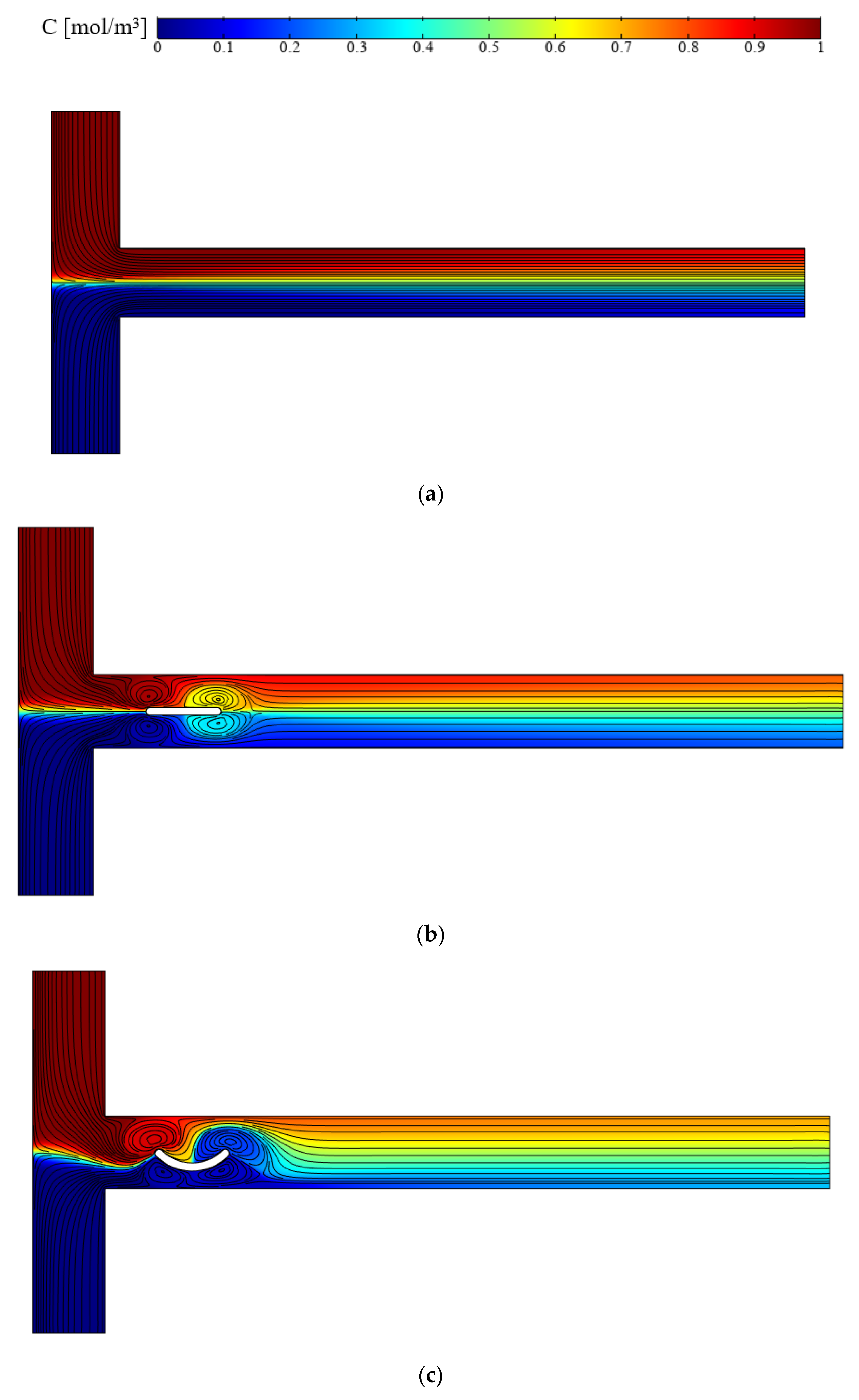
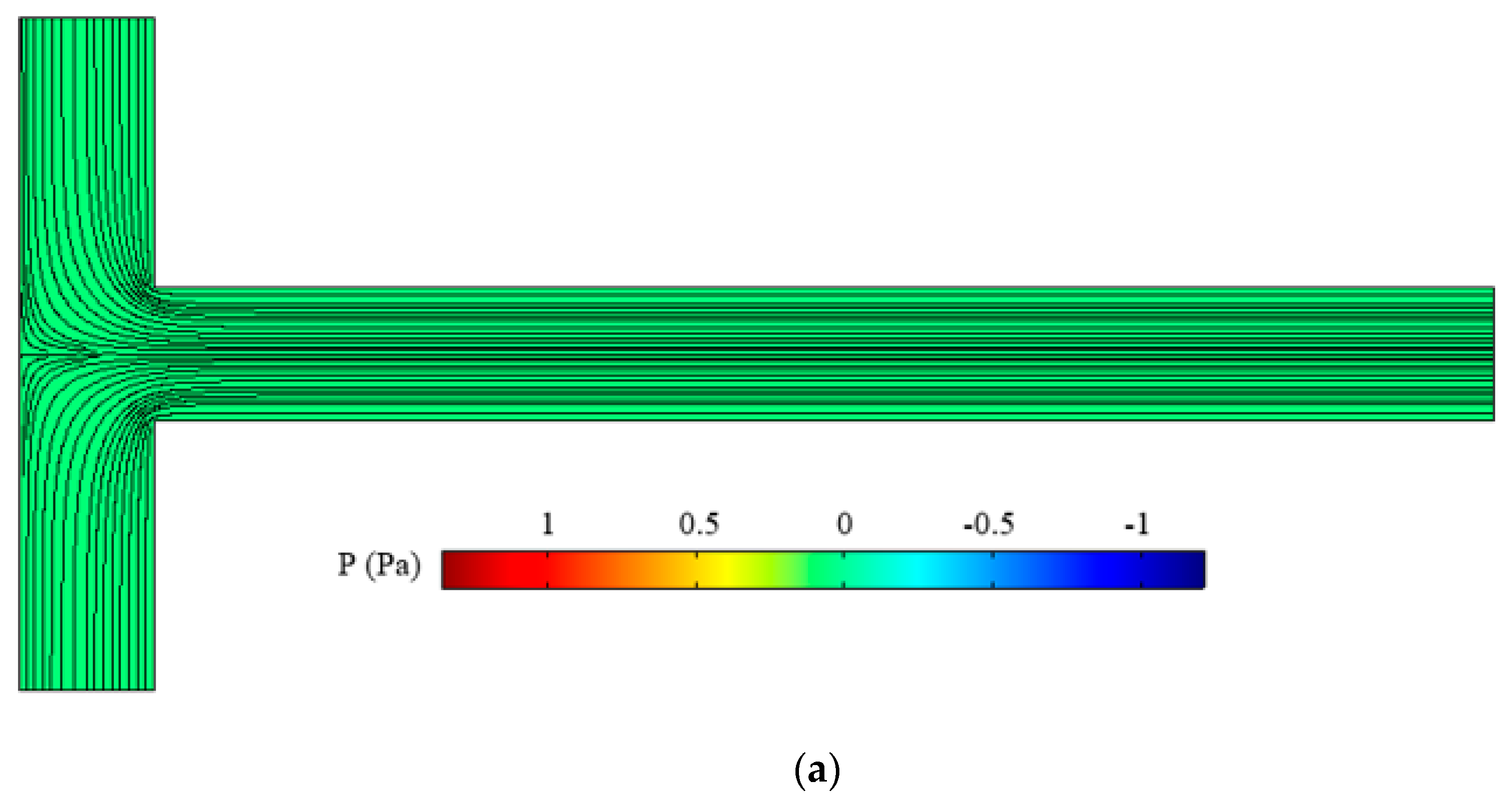
In Figure 6, the flow field and concentration distribution are shown for an applied electric field E = 100 V/cm and for three cases without hurdles, with conducting plate l = W and with conducted curved arc plate sl = W. In the absence of the hurdles, flow is layered and lacks suitable mixing. With the addition of the conducting plate, the flow fields significantly change. Due to the non-uniform and opposite signs of induced zeta potential on the plate, the vorticities are created around it. The vortices created around the plate cause turbulence, allowing for better mixing due to increased contact between the two liquid surfaces [25]. 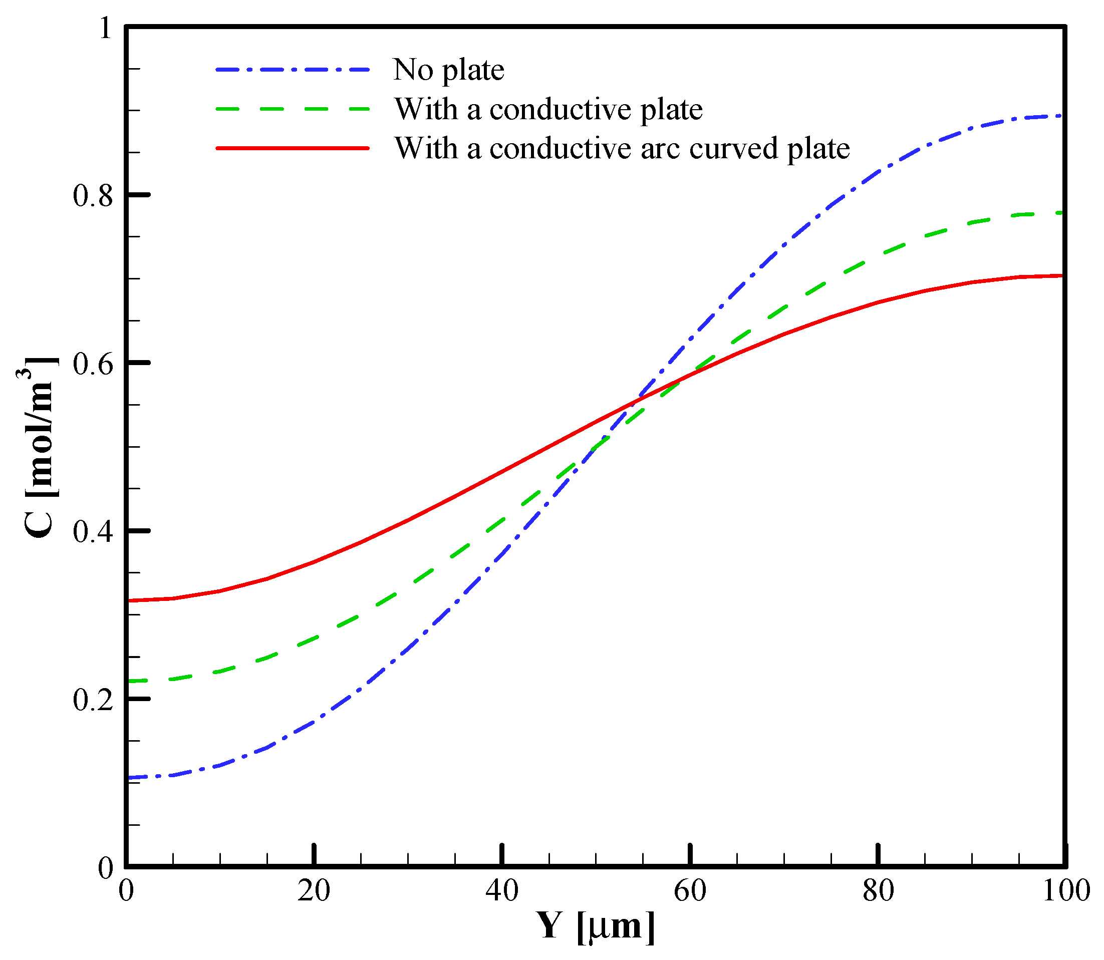In the conductive plate (Figure 6b), the vortices are formed on both sides of the centerline of the microchannel, which is the location of the two-fluid interface, but when the conductive arc curve plate is against the current, the vortices created around the arc curve are larger, and this cuts off the interface between the two flows, thus increasing the mixing relative to the case in which the conductive plate is used against the flow. The concentration patterns in the outlet of the T-micromixer are shown in Figure 7.

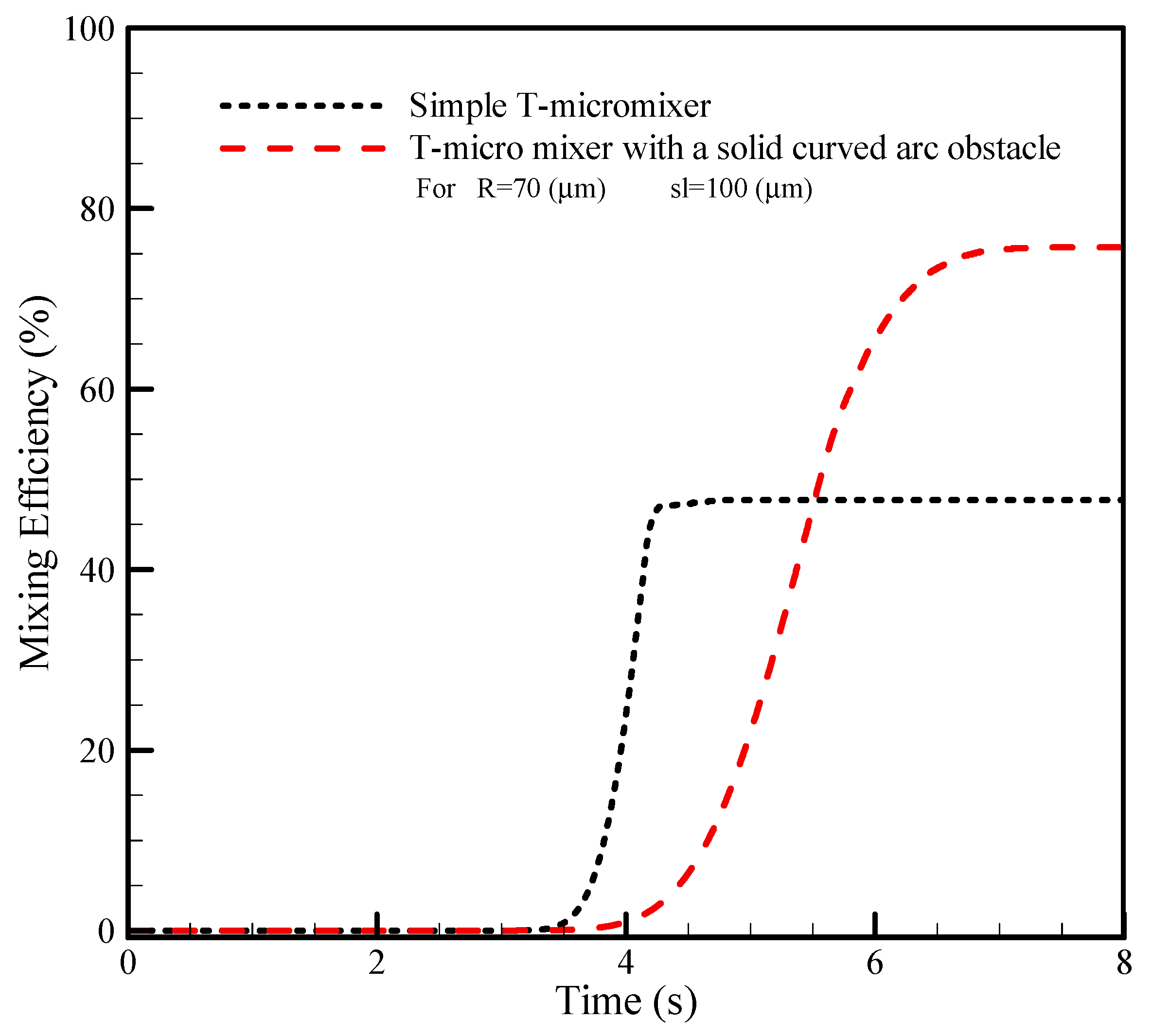
The presence of obstacles and changes in geometry can affect the mixing time. Mixing time in the present micromixer increased due to presence of obstacles and the smaller cross-section of the flow, but the mixing efficiency increased significantly. Figure 8 shows the mixing efficiency based on the time for a simple micromixer and a micromixer with an arc curved plate hurdle. As shown in Figure 8, the presence of the arc curved plate hurdle increases the mixing efficiency by 62% and also increases the mixing time by 41%. This design is practical due to the significant increase in mixing efficiency compared to a simple T-shaped micromixer in applications where mixing quality takes precedence over mixing time [37].

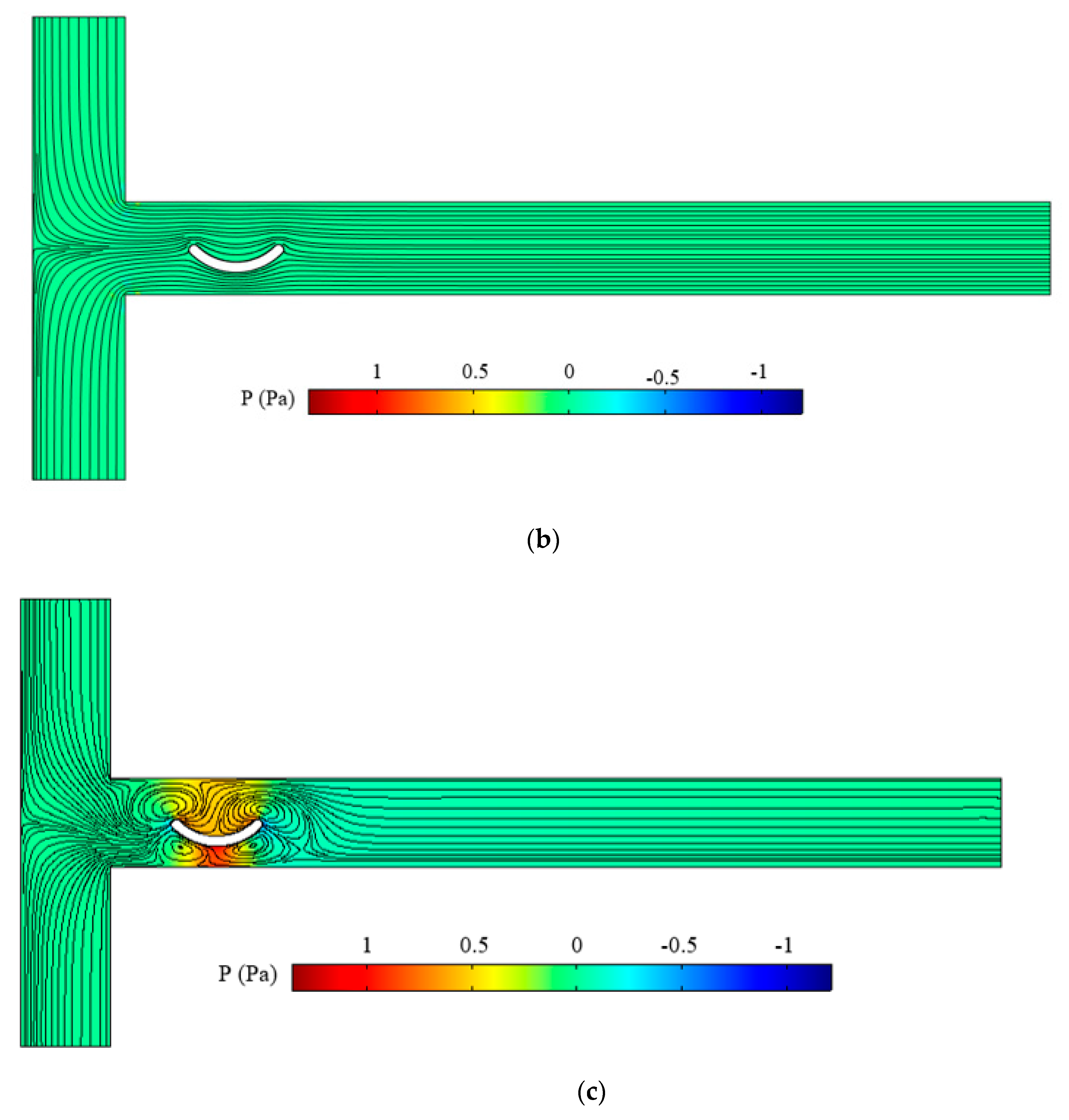
Figure 9 shows the pressure distribution of three models: a simple T-micromixer, a T-micromixer with a non-conductive arc curved plate, and a T-micromixer with a conductive arc curved plate. As can be seen in Figure 9, a pressure gradient is created around the conductive arc curved plate hurdle and inside the flow. In this case, there is a pressure gradient. However, in the case of a non-conducting hurdle, the pressure gradient around the hurdle is small and therefore negligible. According to the flow field around the three models, the flow field changed only around the conductive hurdle, and this caused a higher pressure gradient around the conductive hurdle.

Table 2. Mixing efficiency for three models in Figure 9.

Mixing Efficiency (%)	Model
46.7	Simple T-micromixer
49.9	T-micromixer with non-conductive arc curved plate
75.7	T-micromixer with conductive arc curved plate

provides the mixing efficiency of the three models to determine the effect of the presence of a conductive hurdle on increasing the mixing efficiency. The mixing efficiency in the model with the conductive arc curved plate is approximately 76%, which is higher than the two other cases.

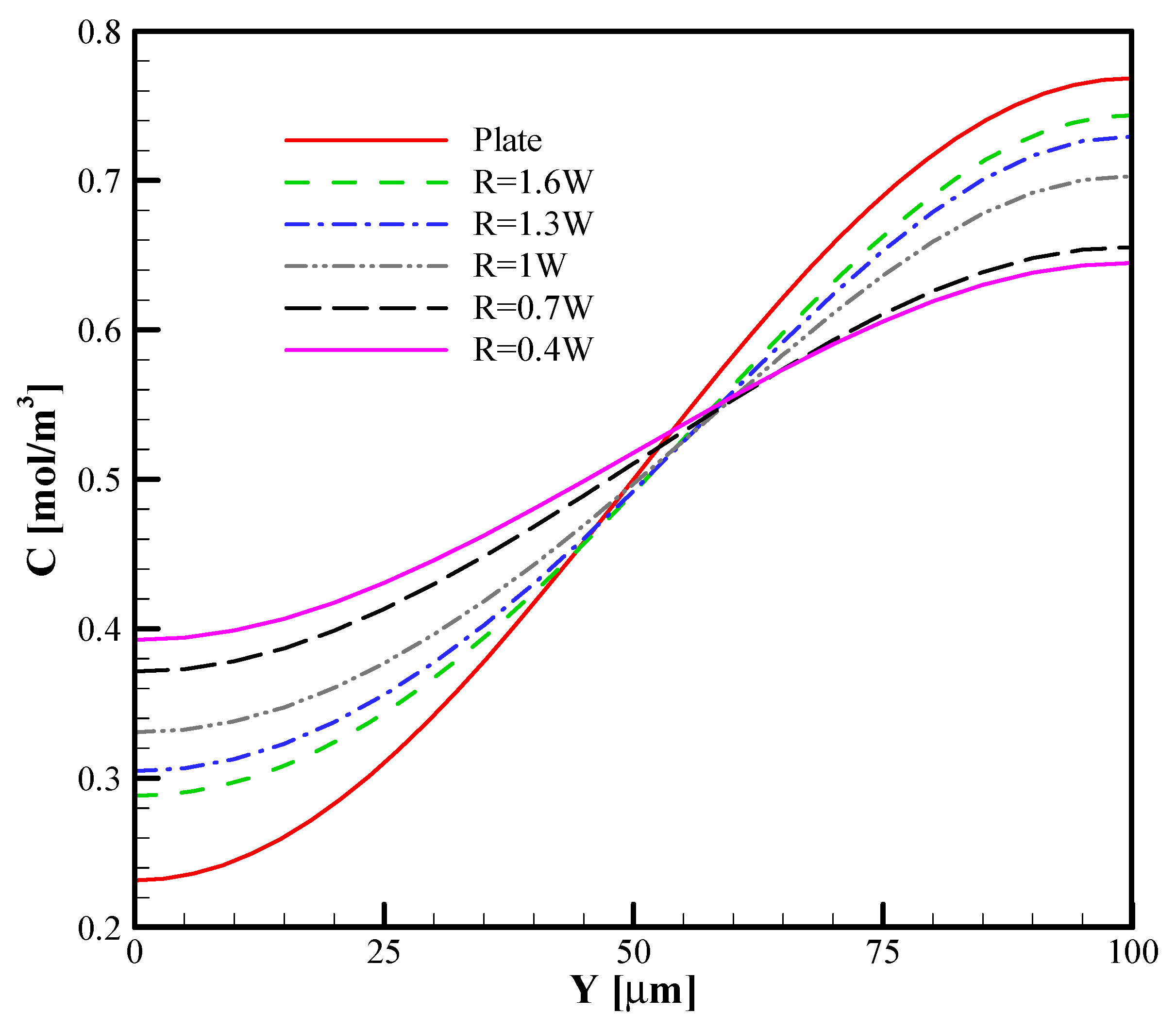
4.2. The Effect of the Radius of the Arc Curve

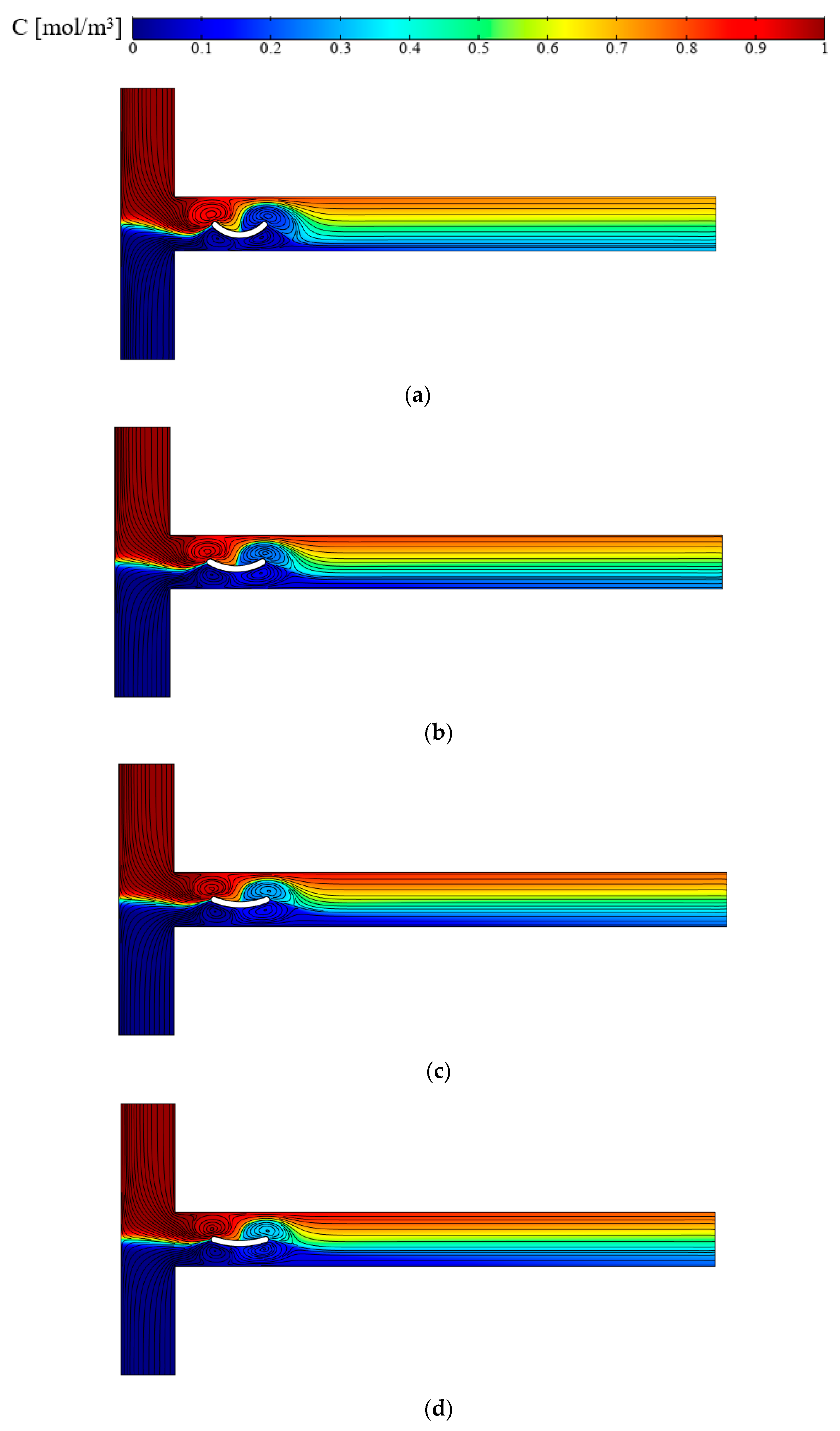
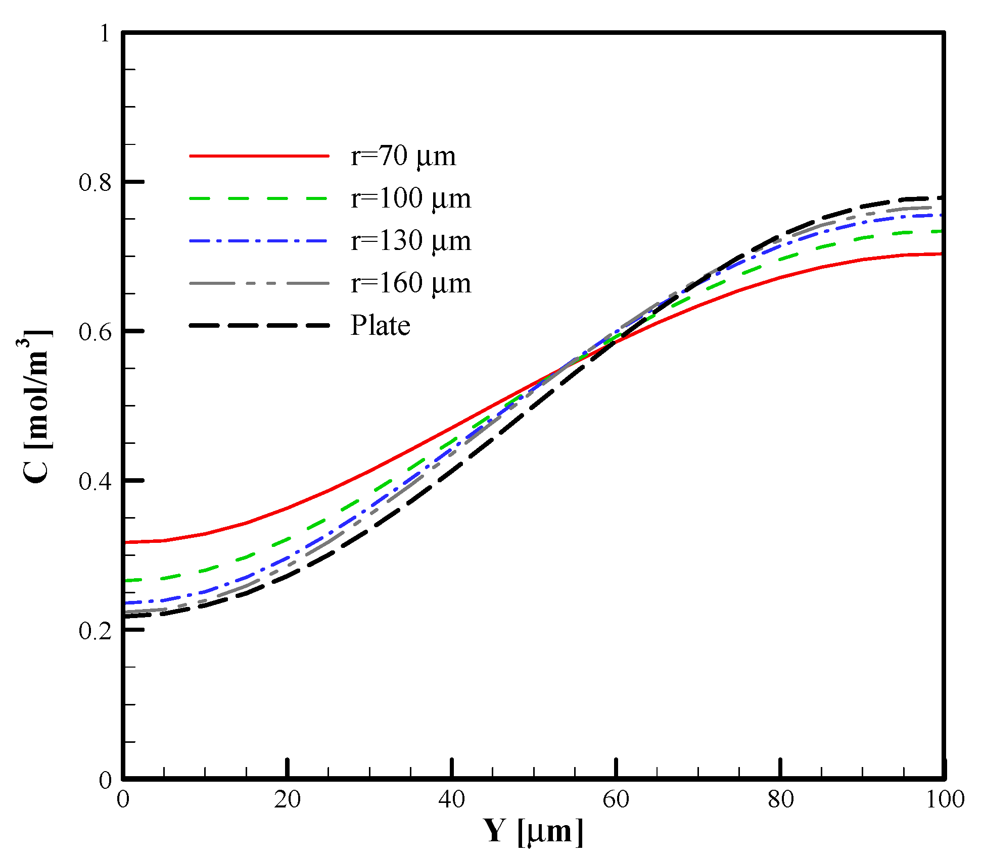
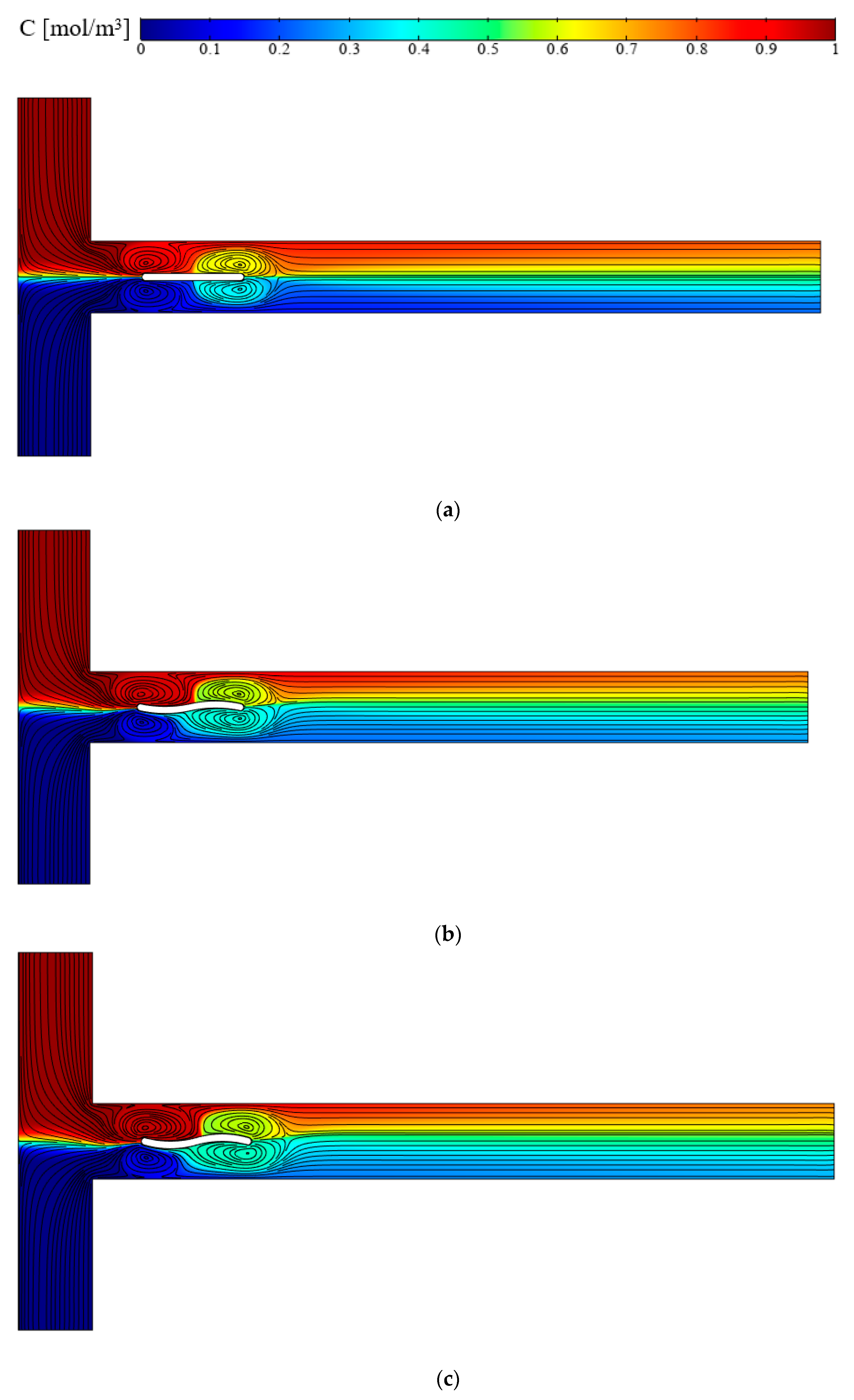
The effect of the radius of the arc curve (R = 0.7 W, R = W, R = 1.3 W, R = 1.6 W) with a constant span length (sl = 100 μm) on the efficiency of the mixing was investigated and is shown in Figure 10. Moreover, for a better comparison of the effect of the presence of the arc curve plate with a plate, a T-micromixer with a conductive plate that was investigated by Nazari et al. [25] (L = 100 μm) is modeled. By analyzing the flow field and concentration distribution along the microchannel, it was observed that the mixing increased with a smaller radius of the curved arc plate. The reason for this is the vortices created around the arc curve placed on either side of the centerline of the channel, which is the interface of the two fluids. As a result, the vortices interrupted the interface of the two liquids and caused better mixing between them, increasing the micromixer’s efficiency. In Figure 11, concentration patterns in the outlet of the micromixer are shown for different radii. By increasing the radius of the arc curve (with constant span length), the mixing efficiency decreased because the vortices had a lesser effect on the interface of the two fluids.

4.3. The Effect of the Span Length of the Arc Curve

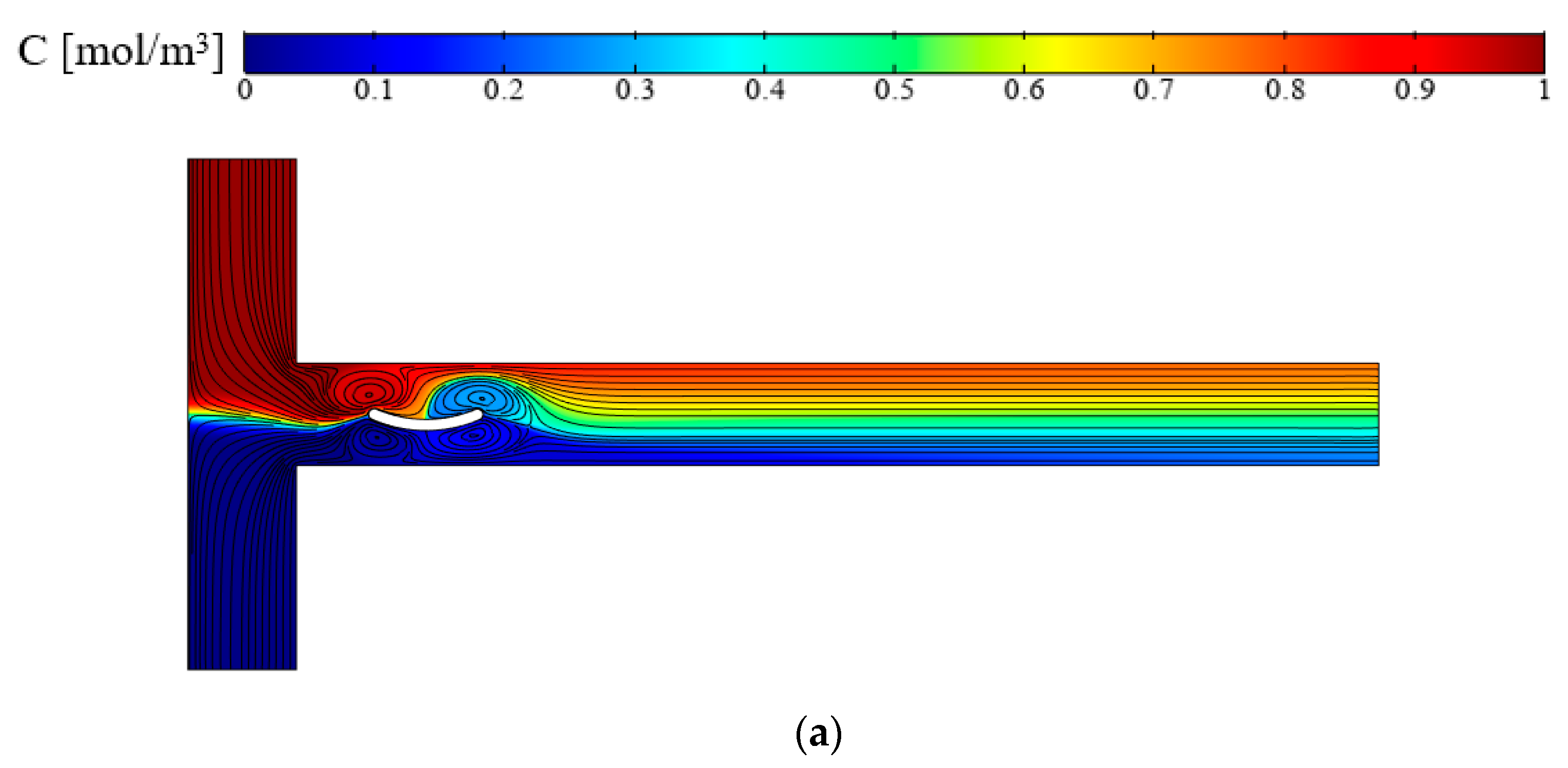
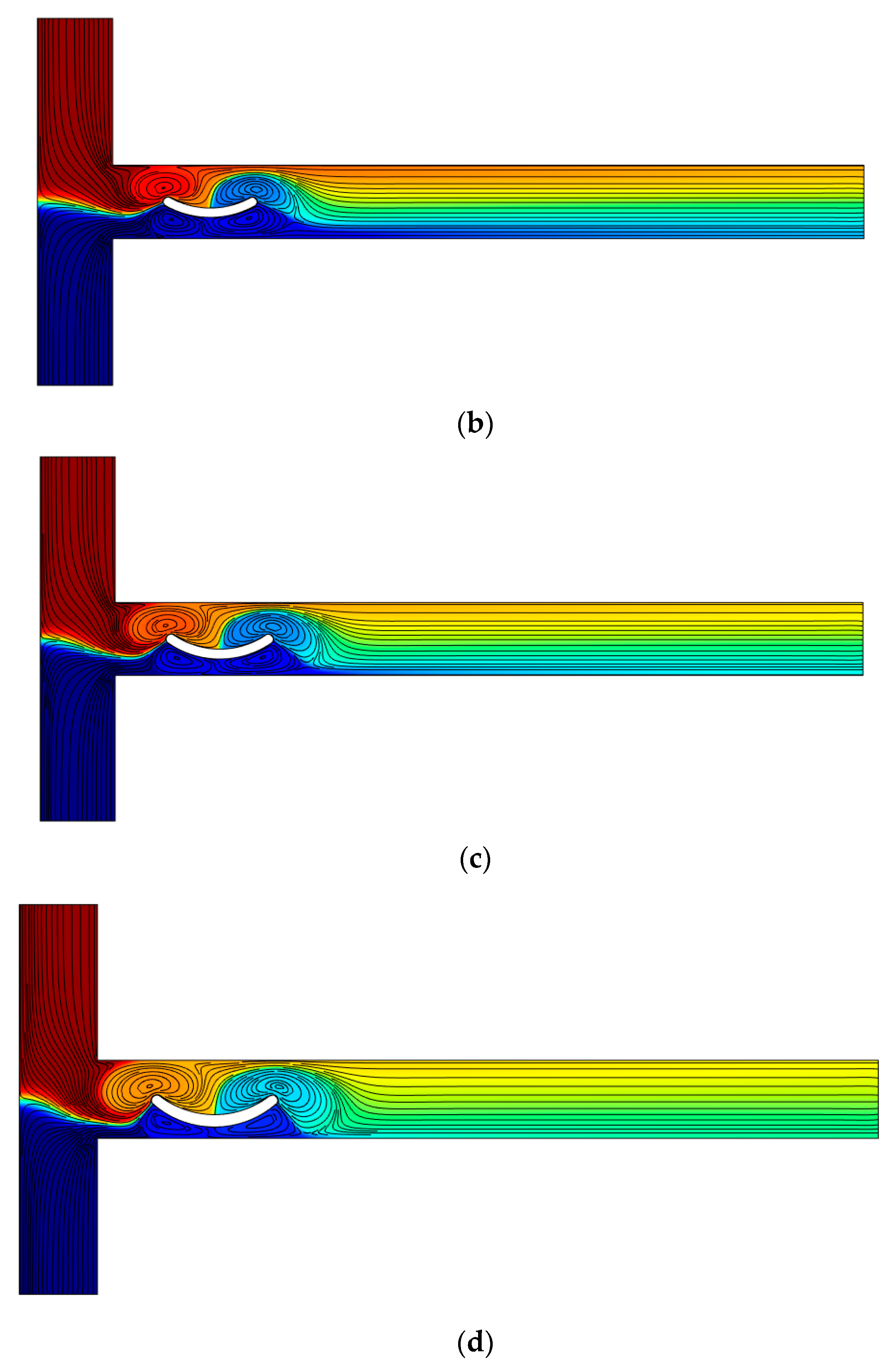
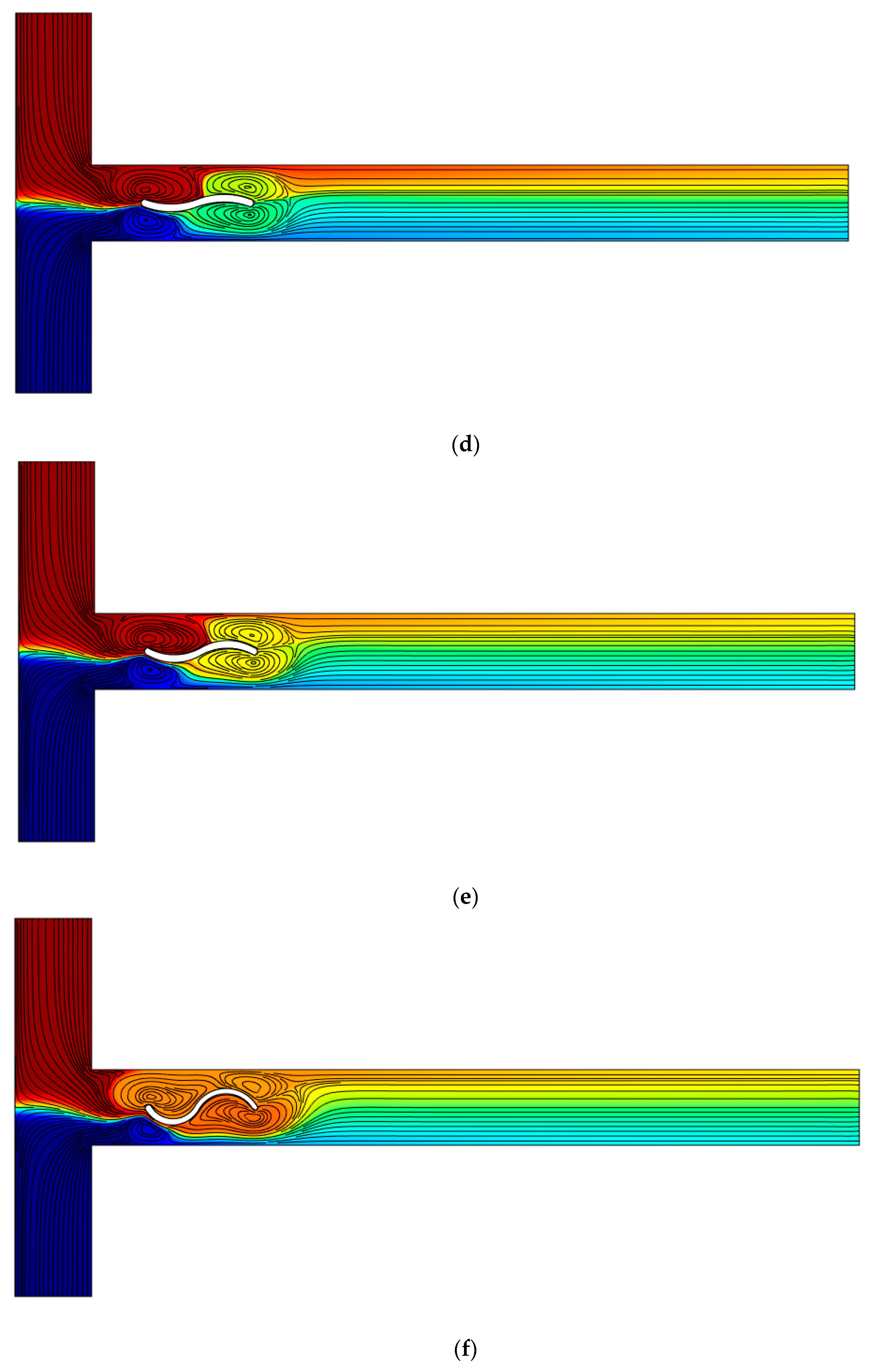
In Figure 12, concentration distribution and streamlines are shown for R = 1.2 W and different span lengths (sl = W, sl = 1.2 W, sl = 1.4 W, sl = 1.6 W). With an increasing span length, the vortices become larger. The increased conducting surface is the cause of the formation of the larger vortices, raising the induced zeta potential. The vortices disrupt the interface of the two liquids, so the mixing is increased. In Figure 12d, the greatest mixing is observed because of the larger vortices and disrupts the interface. In

Table 3. Mixing efficiency for different span lengths of curved arc plate.

Mixing Efficiency (%)	Span Length
67.78	sl = W
75.25	sl = 1.2 W
82.68	sl = 1.4 W
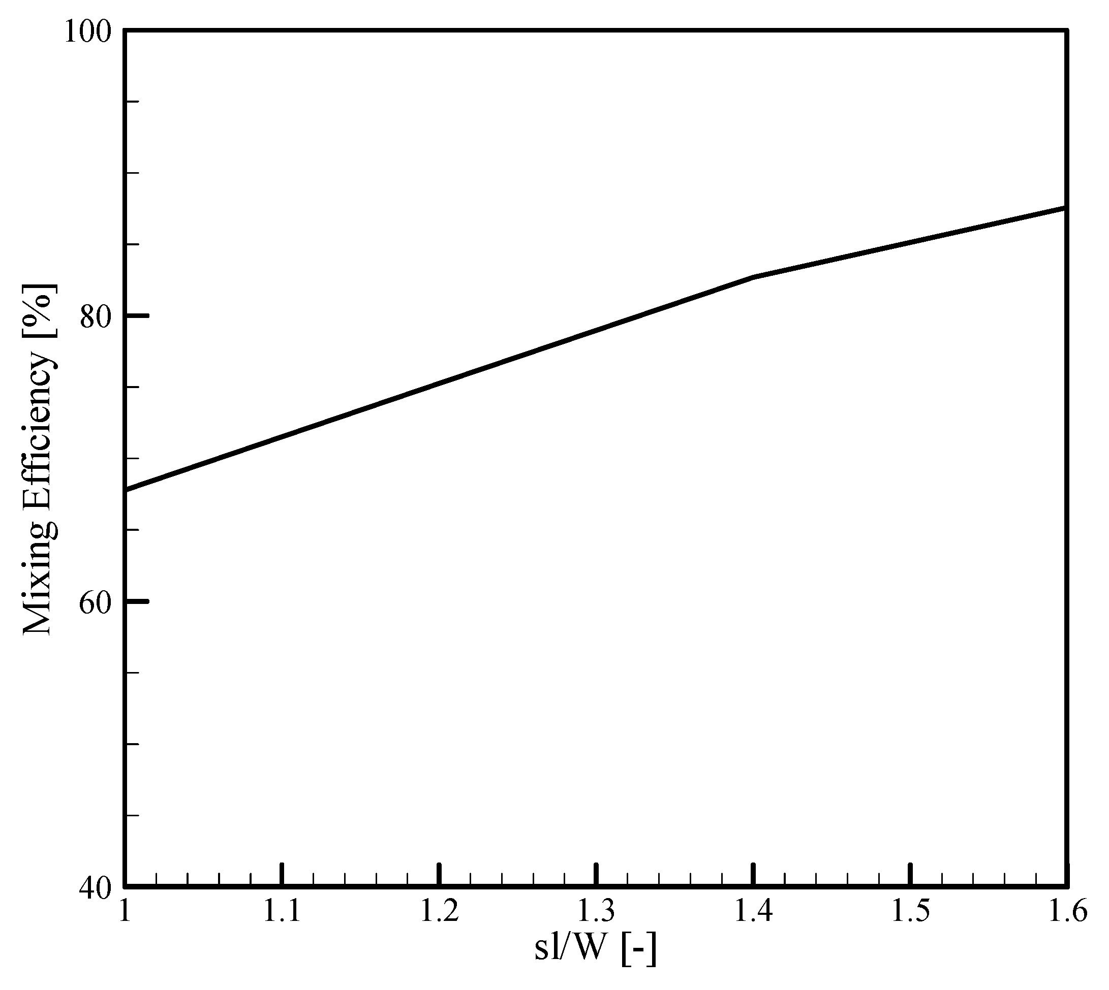
87.58	sl = 1.6 W

and Figure 13, the mixing efficiency at different span lengths is presented. With an increase in the span length by 60%, the mixing efficiency increased by 29.2%.

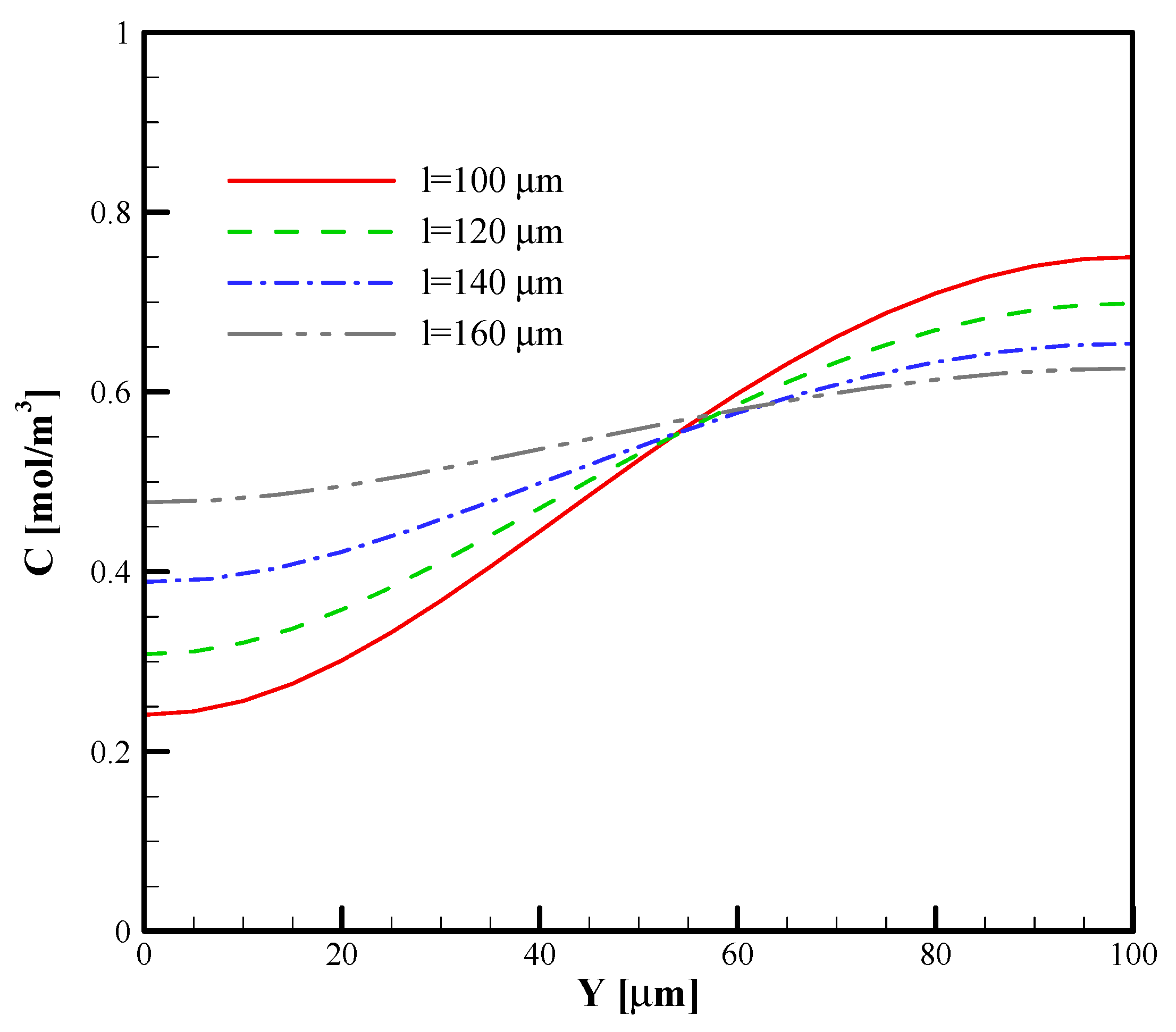
Figure 14 shows the concentration distribution in the outlet of the micromixer for four cases that investigated the effect of the span length of the curved arc plate. Due to the larger vortices and interruption in the area of the interface of the two fluids, with an increase in the span length, the mixing improved.

4.4. The Effect of the Number and Concavity of the Arc Curves

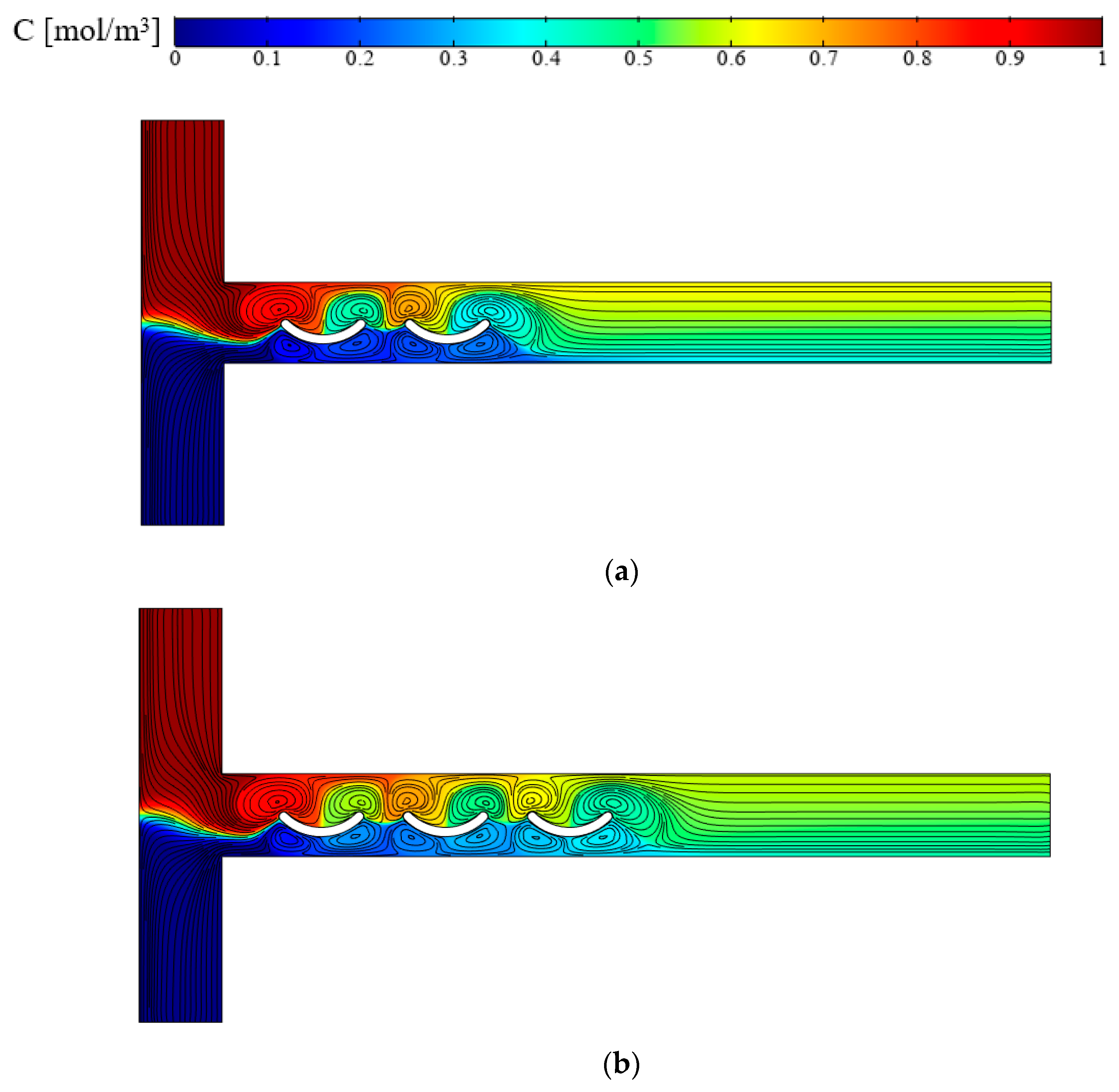
In this section, the effect of the concavity direction of the curved arc plate is examined. In Figure 15, four different cases are presented for R = 0.7 W, sl = 1 W, and E = 100 V⁄cm. With an additional arc curve plate, the mixing efficiency is increased, which is the result of induced vortices. Two patterns are considered for curved arc plates: namely, the case where the concavity direction of the curved arc plates is the same and is upwards, and the other case where the concavity direction of the curved arc plate is alternately upwards and downwards. The mixing efficiency for these four cases is presented in

Table 4. Mixing efficiency for different numbers and concavity directions of curved arc plate.

Mixing Efficiency (%)	Model
87.79	Two curved arc plates in an upward direction
91.86	Three curved arc plates in upward direction concavity
91.93	Two curved arc plates with opposite concave direction
95.44	Three curved arc plates with opposite concave direction

. When the concavity of the curved arc plates is in one direction (Figure 15a,b), the only factor that increases the mixing efficiency is the increase in the number of vortices. However, when the curved arc plates’ concavity is alternately upwards and downwards (Figure 15c,d), the shape of the vortices between the two arc curves is different, and a larger vortex extending to either side of the centerline of the channel increases the mixing. The creation of this vortex is due to the different directions of the arc curves. According to Table 4, in the case of two curved arc plates with opposite concave direction, the mixing efficiency is higher than in the case of three curved arc plates in upward direction concavity. Maximum efficiency was achieved for the three curved arc plates with opposite concave directions. The geometric pattern of the obstacle within the flow in the present work with fewer obstacles leads to a better mixing efficiency than in the study of Farahinia and Zhang [38]. Furthermore, similar to Nazari et al. [25], as the number of obstacles increases, the vortex production increases, thus increasing the mixing efficiency.

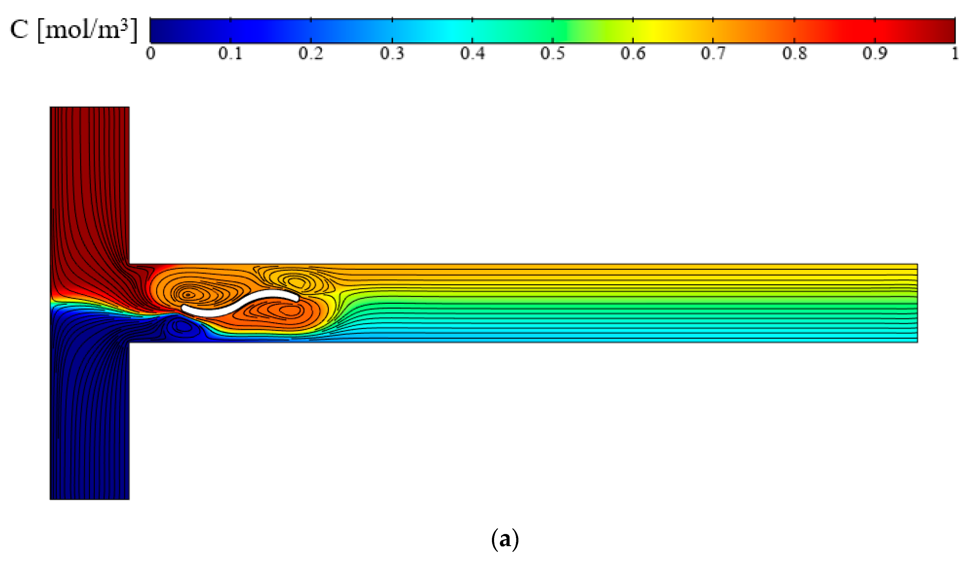
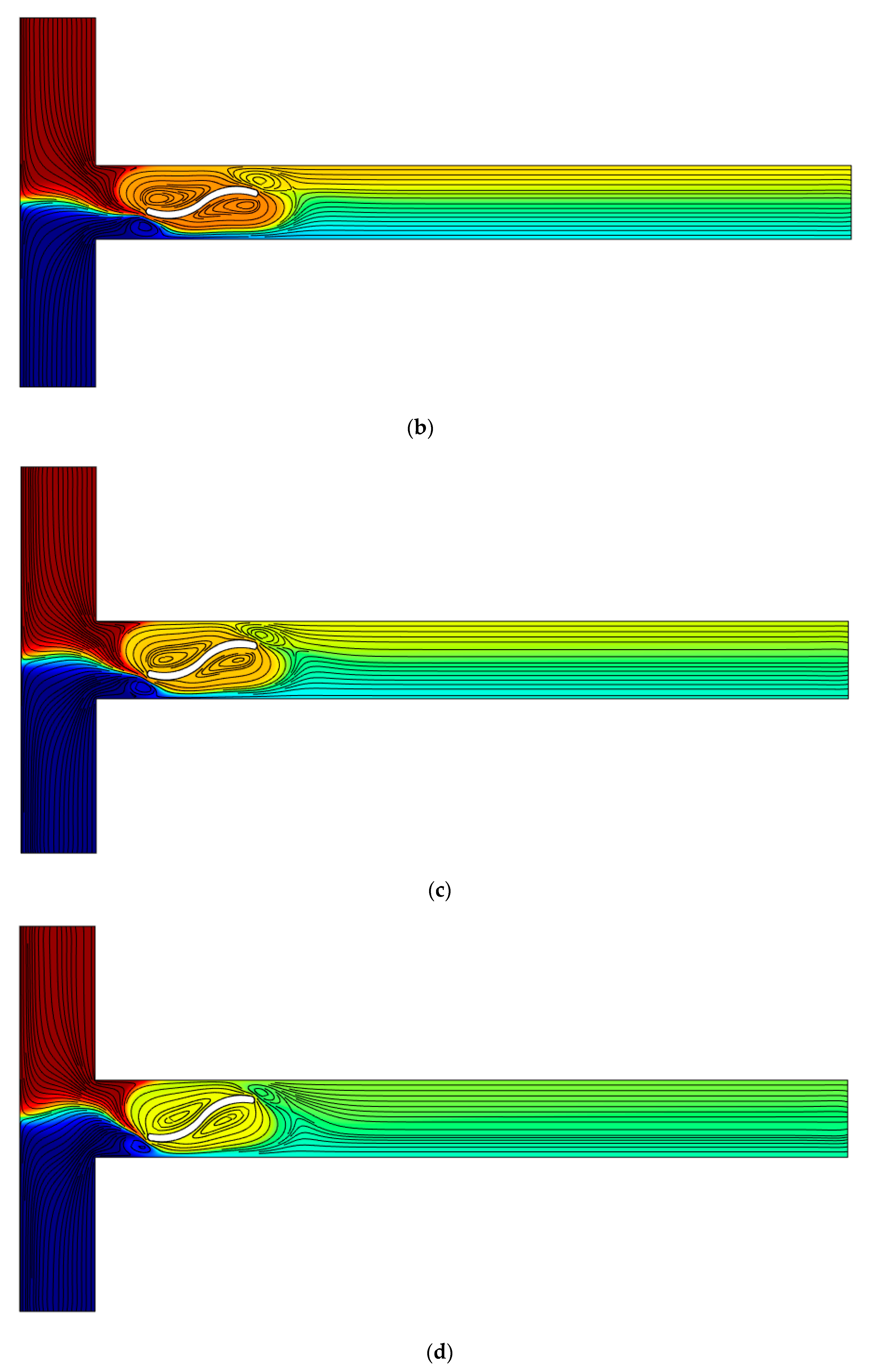
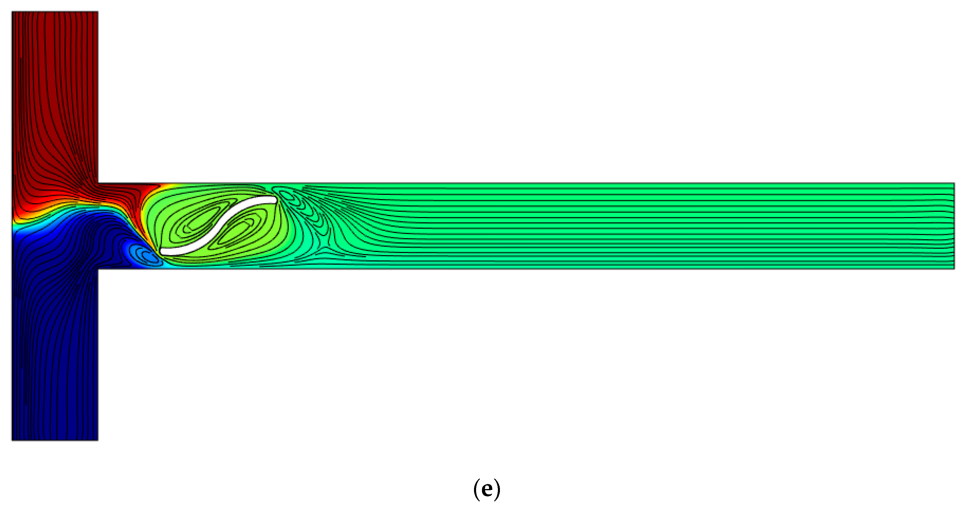
4.5. Two Curved Arc Plates

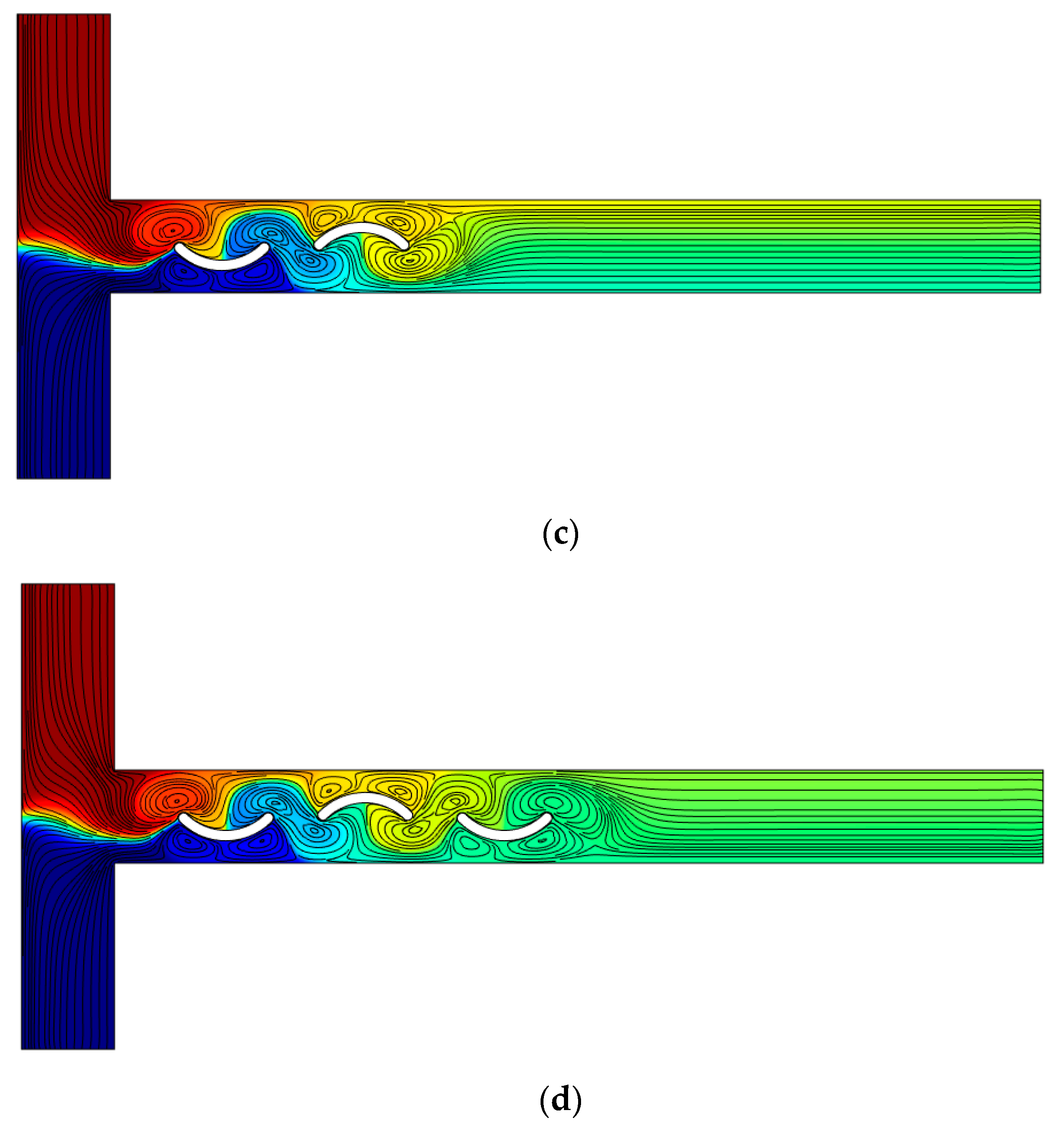
The presence of vortices improves the mixing process. The plate geometry can be changed to create a larger vortex. As shown in this section, by changing the geometry of the plate to a curve with two opposite concavities, larger and more elongated vortices can be achieved, and the effect of using two curved arc plates in a continuous curve with two arcs in opposite concavity directions (upwards and downwards) with span length sl = 1.4 W was investigated. In Figure 16, streamlines and concentration distribution for different radius (R = 0.4 W, R = 0.7 W, R = W, R = 1.3 W, R = 1.6 W) are presented. According to Figure 16, by changing the plate with two curved arc plates and reducing the radius, the mixing is improved. With the creation of curvature, the vortices created around these two curved arc plates become larger, and with a reduction in the radius from R = 1.6 W to R = 0.4 W, these vortices disturb the interface and improve the mixing. For a better explanation, the concentration distribution in the micromixer outlet for various radii is shown in Figure 17. The mixing efficiency for a plate and two curved arc plates with R = 0.4 W is 65.8% and 84%, respectively.

4.6. The Effect of the Conductive Curved Arc Plate Orientation Angle

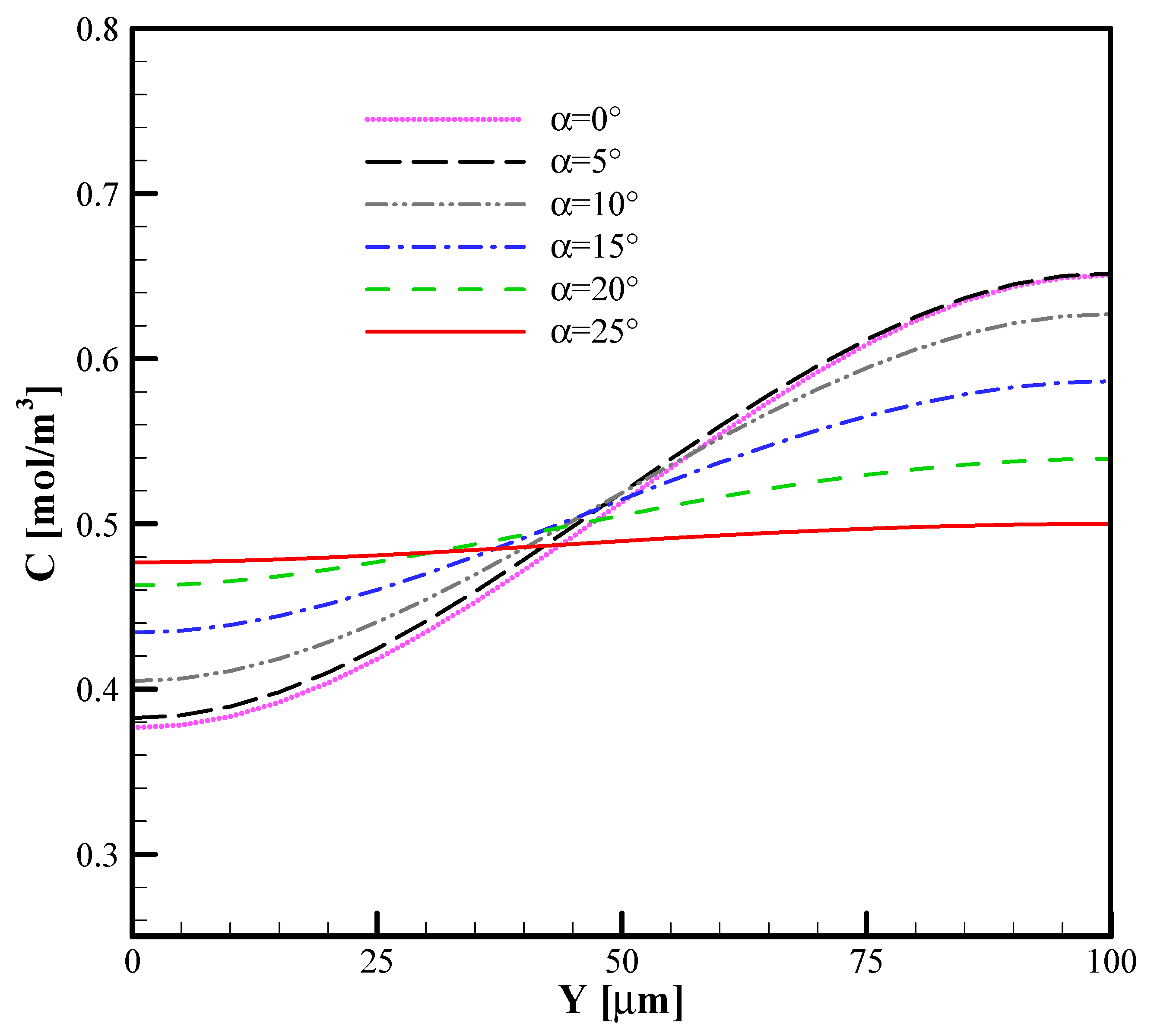
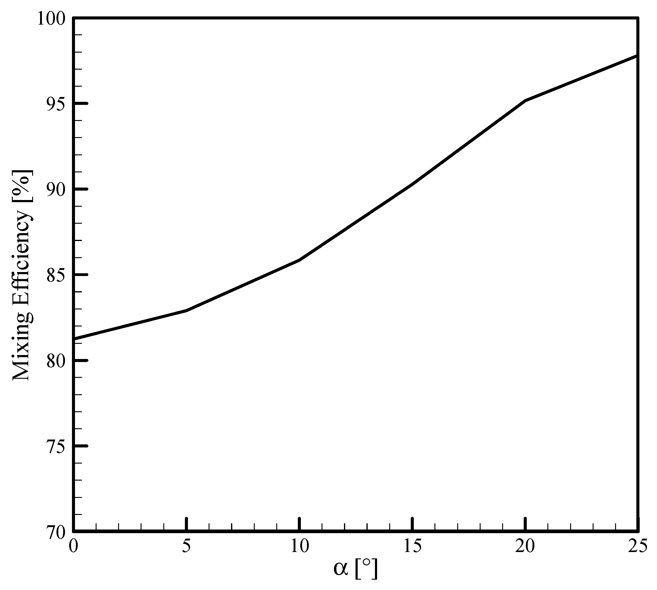
In Figure 18, the effect of the orientation angle of the two curved arc plates on the streamlines and concentration distribution is shown for E = 100 V/cm, R = 0.7 W, sl = 0.7 W. With an increasing orientation angle of the two curved arc plates, the shape of the vortices changes. The vortices at the beginning and end of the two curved arc plates become smaller, and the vortices along the two curved arc plates become larger. In addition, with an increasing orientation angle from 5 to 25, the vortices created along the two curved arc plates interrupt the centerline of the microchannel and interface of the two fluids and improve the efficiency. In Figure 19, the concentration distribution for different orientation angles in the outlet of the microchannel is shown. According to Figure 20, with an increasing orientation angle, the mixing improves. The mixing efficiency for α = 0° and α = 25° is 81% and 97.8%, respectively. The results of the effect of the conductive curved arc plate orientation angle on the mixing efficiency are similar to those of Nazari et al. [25].

4.7. The Effect of the Diffusion Coefficient

In

Table 5. Mixing efficiency for various orders of the diffusion coefficient.

Mixing Efficiency (%)	Order of Diffusion Coefficient
95.4358	10−10
92.1206	10−11
91.3940	10−12

, the mixing efficacy for three diffusion coefficients is presented. Three curved arc plates with alternate upwards and downwards patterns are considered to investigate this geometry’s performance when the diffusion coefficient is low. In this case, according to Equation (22), the mixing efficiency is above 90%, which is due to the large vortices. Thus, the mixing performance has clearly improved.

5. Conclusions

In this research, a computational fluid dynamics analysis was conducted on an induced-charge electrokinetic micromixer. In past studies, a simple conductive plate or other non-conductive obstacles, such as plate, circle, and rectangle, were investigated, but in this paper, the conductive arc curved plate was used. By inducing non-uniform zeta potential on the curved arc plate, vortices were induced inside the channel and improved mixing. In a systematic investigation, the effect of the arc radius, span length, number of curved arc plates, the direction of concavity, and the orientation angle of curved arc plates was examined. The outcomes were plotted in the form of streamlines, outlet concentration distribution, and mixing efficiency. The main results can be summarized as follows:

• Changing the conductive plate to a conductive curved arc plate changes the shape of induced vortices and thus increases the mixing efficiency by 17.35%.
• By increasing the span length by 60%, the mixing efficacy rises by 30%.
• A growth in the number of curved arc plates increases the number of vortices and so increases the mixing efficacy.
• The mixing efficacy increases by decreasing the radius. At a lower radius, the vortices are drawn toward the centerline of the microchannel. In this case, the vortices improve the mixing performance by disrupting the interface between the two fluids.
• The direction of concavity in the curved arc plate affects the quality of mixing. In the case of using three curved arc plates in one direction, the mixing efficiency is 91.86%, and by changing the concavity direction to an upwards and downwards pattern, the mixing efficiency reaches 95.44%.
• By varying the placement angle from 0 to 25, the mixing efficiency is improved by 19.2%.
• The performance of three curved arc plates with an alternate upwards and downwards pattern of concavity for a lower diffusion coefficient was investigated and led to a mixing efficiency above 90%.