Article

Bright–Dark Soliton Waves’ Dynamics in Pseudo Spherical Surfaces through the Nonlinear Kaup–Kupershmidt Equation

by
Mostafa M. A. Khater
1,2,*,†,
Lanre Akinyemi
3,†,
Sayed K. Elagan
4,†,
Mohammed A. El-Shorbagy
5,6,†,
Suleman H. Alfalqi
7,†,
Jameel F. Alzaidi
7,† and
Nawal A. Alshehri
4,†
1
Department of Mathematics, Faculty of Science, Jiangsu University, Zhenjiang 212013, China
2
Department of Mathematics, Obour Institutes, Cairo 11828, Egypt
3
Department of Mathematics, Prairie View A & M University, Prairie View, TX 77446, USA
4
Department of Mathematics, Faculty of Science, Taif University, P.O. Box 11099, Taif 21944, Saudi Arabia
5
Department of Mathematics, College of Science and Humanities in Al-Kharj, Prince Sattam bin Abdulaziz University, Al-Kharj 11942, Saudi Arabia
6
Department of Basic Engineering Science, Faculty of Engineering, Menoufia University, Shebin El-Kom 32511, Egypt
7
Department of Mathematics, Faculty of Science and Arts, Mahayil Asir King Khalid University, Abha 61421, Saudi Arabia
*
Author to whom correspondence should be addressed.
These authors did all this work equally.
Submission received: 28 March 2021 / Revised: 26 April 2021 / Accepted: 8 May 2021 / Published: 28 May 2021

Abstract

:
The soliton waves’ physical behavior on the pseudo spherical surfaces is studied through the analytical solutions of the nonlinear (1+1)–dimensional Kaup–Kupershmidt ( KK ) equation. This model is named after Boris Abram Kupershmidt and David J. Kaup. This model has been used in various branches such as fluid dynamics, nonlinear optics, and plasma physics. The model’s computational solutions are obtained by employing two recent analytical methods. Additionally, the solutions’ accuracy is checked by comparing the analytical and approximate solutions. The soliton waves’ characterizations are illustrated by some sketches such as polar, spherical, contour, two, and three-dimensional plots. The paper’s novelty is shown by comparing our obtained solutions with those previously published of the considered model.

1. Introduction

A significant and prominent portion of the nonlinear partial differential Equation (NLPDE) has recently played a role in describing many physical, chemical, biological, mechanical, optical, and other phenomena in engineering [1,2]. This image aims to identify the new features of each model by finding their moving wave solutions to construct the original and soundscapes for semi-analytical and numerical schemes [3,4,5]. Therefore, the analytical findings’ precision can be verified by contrasting the analytical to estimated solutions for displaying the matching results [6,7]. Thus, several mathematicians and physics researchers have focused on the drawing up of accurate analytical, semi–analytical, and numerical schemes such as Khater method, modified Khater method, generalized Khater method, exp–function method, Hirota’s method, the bi–linear method, Adomian degradation method, b-spline schemes, and the Sine Gordon expansion method [8,9,10,11,12,13,14,15]. These schemes have dealt with many phenomena and some novel properties that allow many great applications [16,17,18,19,20] to use these solutions.
This research paper investigates the analytical and approximate solutions of (1+1)–D KK equation through the modified F–expansion (MFE), Novel auxiliary Equation (NAE), and variational iteration (VI) methods [21,22,23,24,25]. This model is given by [26,27,28,29,30]
q 1 K t + K 5 x + q 2 K K x   x   x + q 3   K x K x   x + q 4 K 2 K x = 0 ,
where q g , g = 1 , 2 , 3 , 4 are arbitrary constants applying the following wave traveling transformation K ( x , t ) = R ( G ) ,   G = x + λ   t , where λ is the arbitrary constant to be evaluated through the suggested analytical methods, converts the NLPDE into the following ordinary differential Equation (ODE)
R ( 5 ) + q 2   R ( 3 )   R + λ   q 1   R + q 3   R   R + q 4   R 2   R = 0 .
Applying the homogeneous balance principles to Equation (2) for evaluating the value of balance between the ODE’s model form, finds that s = 2 . Consequently, the considered model’s general solutions are given by
R G = i = s n a i   ( Q ( G ) + ϱ ) i = a 2   ( Q ( G ) + ϱ ) 2 + a 1   ( Q ( G ) + ϱ ) + a 0 , i = 1 s a i   Λ ( G ) i + a 0 = a 2   Λ ( G ) 2 + a 1   Λ ( G ) + a 0 ,
where s is the value of balance, while a 2 ,   a 1 ,   a 0 are arbitrary constants to be evaluated along with the suggested methods’ framework.
The remaining parts of the article are provided in the order below; Section 2 offers the wave’s solitary versions by introducing the analytical schemes indicated. The analytical solutions obtained are often examined to achieve the requested criteria for applying the semi-analytical methods suggested. Finally, the estimated solutions are determined, and analytical, semi-analytical, and total errors between the solutions are shown. Specific alternatives are displayed by sure distinct illustrations that demonstrate the novel properties of the model. The findings and creativity of the paper are seen in Section 3. The description of all results obtained in the whole study paper is explained in Section 4.

2. Distinct Solutions

Here, many various kinds of solutions are obtained and employ two recent analytical schemes then using their solutions for evaluating the approximate solutions of the considered model. This investigation aims to illustrate the dynamical behavior of the soliton waves on pseudo-spherical surfaces. Additionally, it seeks to show the accuracy of the obtained solutions by estimating the value of error between both solutions.

2.1. Soliton Wave Solution

Employing the suggested computational (MFE and NAE) methods investigates the solitary wave solutions of the proposed model.

2.1.1. MFE Method’s Investigation

Employing the MFE method’s framework with the following auxiliary equation Q ( G ) = Q ( G ) 2 + ϱ , where ϱ is arbitrary constant, and the above-mention general solution, finds the following value of the previous-shown parameters:
  • Set A
    a 0 = 1 3 a 2 ϱ ( 3 ϱ + 2 ) , a 1 = 2 a 2 ϱ , q 1 = ϱ 2 a 2 2 q 4 + 12 a 2 q 2 + 144 9 λ , q 3 = a 2 q 4 6 60 a 2 2 q 2 .
  • Set B
    a 1 = 12 q 2 ϱ q 4 , a 2 = 6 q 2 q 4 , q 1 = 4 q 4 ϱ a 0 q 2 ( 3 ϱ + 2 ) + 4 ϱ + a 0 2 q 4 2 + 12 q 2 2 ϱ 2 ( ϱ + 1 ) ( 3 ϱ + 1 ) λ q 4 , q 3 = 10 q 4 q 2 q 2 .
Thus, the solitary solution’s of the nonlinear (1+1)–D KK equation are given by For ϱ < 0 , we have
K A , 1 ( x , t ) = a 2 ϱ tan 2 ϱ ( λ t + x ) + 2 ϱ 3 + a 1 ϱ tan ϱ ( λ t + x ) + ϱ + a 2 ϱ tan ϱ ( λ t + x ) + ϱ 2 ,
K A , 2 ( x , t ) = 1 3 a 2 ϱ 3 cot 2 ϱ ( λ t + x ) + 2 + a 1 ϱ ϱ cot ϱ ( λ t + x ) + a 2 ϱ ϱ cot ϱ ( λ t + x ) 2 ,
K B , 1 ( x , t ) = a 1 ϱ tan ϱ ( λ t + x ) + ϱ + a 2 ϱ tan ϱ ( λ t + x ) + ϱ 2 + a 0 + 6 q 2 ϱ ϱ tan 2 ϱ ( λ t + x ) q 4 ,
K A , 2 ( x , t ) = a 1 ϱ ϱ cot ϱ ( λ t + x ) + a 2 ϱ ϱ cot ϱ ( λ t + x ) 2 + a 0 + 6 q 2 ϱ ϱ cot 2 ϱ ( λ t + x ) q 4 .
For ϱ > 0 , we have
K A , 3 ( x , t ) = a 2 ϱ tan 2 ϱ ( λ t + x ) + 2 ϱ 3 + a 2 ϱ tan ϱ ( λ t + x ) + ϱ 2 + a 1 ϱ tan ϱ ( λ t + x ) + ϱ ,
K A , 4 ( x , t ) = 1 3 a 2 ϱ 3 cot 2 ϱ ( λ t + x ) + 2 + a 2 ϱ ϱ cot ϱ ( λ t + x ) 2 + a 1 ϱ ϱ cot ϱ ( λ t + x ) ,
K B , 3 ( x , t ) = a 1 ϱ tan ϱ ( λ t + x ) + ϱ + a 2 ϱ tan ϱ ( λ t + x ) + ϱ 2 + a 0 + 6 q 2 ϱ ϱ tan 2 ϱ ( λ t + x ) q 4 ,
K B , 4 ( x , t ) = a 1 ϱ ϱ cot ϱ ( λ t + x ) + a 2 ϱ ϱ cot ϱ ( λ t + x ) 2 + a 0 + 6 q 2 ϱ ϱ cot 2 ϱ ( λ t + x ) q 4 .
For ϱ = 0 , we have
K A , 5 ( x , t ) = a 2 1 λ t + x ϱ 2 + a 1 ϱ 1 λ t + x + a 2 1 ( λ t + x ) 2 + 2 ϱ 3 ,
K B , 5 ( x , t ) = a 2 1 λ t + x ϱ 2 + a 1 ϱ 1 λ t + x + a 0 + 6 q 2 ϱ 2 1 ( λ t + x ) 2 q 4 .

2.1.2. NAE Method’s Soliton Solutions

Employing the NAE method’s framework with the following auxiliary equation Λ ( Q ) = P 3   Λ ( Q ) 2 + P 2   Λ ( Q ) + P 1 , where P j , j = 1 , 2 , 3 are arbitrary constants, and the above-mentioned general solution, give the following value of the previously shown parameters:
  • Set A
    a 0 a 2 P 2 2 + 8 P 1 P 3 12 P 3 2 , a 1 a 2 P 2 P 3 , q 1 P 2 2 4 P 1 P 3 2 12 a 2 P 3 2 q 2 + a 2 2 q 4 + 144 P 3 4 144 λ P 3 4 , q 3 a 2 q 4 6 P 3 2 60 P 3 2 a 2 2 q 2 .
  • Set B
    a 1 6 P 2 P 3 q 2 q 4 , a 2 6 P 3 2 q 2 q 4 , q 1 1 λ q 4 ( q 4 a 0 P 2 2 + 8 P 1 P 3 q 2 + P 2 2 4 P 1 P 3 2 + a 0 2 q 4 2 + 6 P 1 P 3 P 2 2 + 2 P 1 P 3 q 2 2 ) , q 3 10 q 4 q 2 q 2 .
Thus, the solitary solutions of the nonlinear (1+1)–D KK equation are given by
For P 2 2 4 P 1 P 3 > 0 ,   P 2 P 3 0 , we get
K A , 1 ( x , t ) = a 2 P 2 2 4 P 1 P 3 12 P 3 2 3   sech 2 1 2 P 2 2 4 P 1 P 3 ( λ t + x ) 1 ,
K A , 2 ( x , t ) = a 2 P 2 2 4 P 1 P 3 12 P 3 2 3   csch 2 1 2 P 2 2 4 P 1 P 3 ( λ t + x ) + 1 ,
K B , 1 ( x , t ) = a 0 + 3 q 2 2 q 4 4   P 1 P 3 + P 2 2 4 P 1 P 3 sech 2 1 2 P 2 2 4 P 1 P 3 ( λ t + x ) ,
K B , 2 ( x , t ) = a 0 + 3 q 2 2 q 4 4   P 1 P 3 P 2 2 4 P 1 P 3 csch 2 1 2 P 2 2 4 P 1 P 3 ( λ t + x ) .
For P 2 2 4 P 1 P 3 < 0 ,   P 2 P 3 0 , we get
K A , 3 ( x , t ) = a 2 P 2 2 4 P 1 P 3 12 P 3 2 3 sec 2 1 2 4 P 1 P 3 P 2 2 ( λ t + x ) 1 ,
K A , 4 ( x , t ) = a 2 P 2 2 4 P 1 P 3 12 P 3 2 3 csc 2 1 2 4 P 1 P 3 P 2 2 ( λ t + x ) 1 ,
K B , 3 ( x , t ) = a 0 + 3 q 2 2 q 4 4 P 1 P 3 + P 2 2 4 P 1 P 3 sec 2 1 2 4 P 1 P 3 P 2 2 ( λ t + x ) ,
K B , 4 ( x , t ) = a 0 + 3 q 2 2 q 4 4 P 1 P 3 + P 2 2 4 P 1 P 3 csc 2 1 2 4 P 1 P 3 P 2 2 ( λ t + x ) .
For P 2 2 4 P 1 P 3 > 0 ,   P 1 P 3 0 , we get
K A , 5 ( x , t ) = a 2 P 2 2 4 P 1 P 3 ( 10 P 1 P 3 + P 2 2 4 P 1 P 3 P 2 sinh P 2 2 4 P 1 P 3 ( λ t + x ) + P 2 2 2 P 1 P 3 cosh P 2 2 4 P 1 P 3 ( λ t + x ) ) / ( 12 P 3 2 ( P 2 cosh ( 1 2 P 2 2 4 P 1 P 3 ( λ t + x ) ) P 2 2 4 P 1 P 3 sinh 1 2 P 2 2 4 P 1 P 3 ( λ t + x ) ) 2 ) ,
K A , 6 ( x , t ) = a 2 P 2 2 4 P 1 P 3 ( 10 P 1 P 3 + P 2 2 4 P 1 P 3 P 2 sinh P 2 2 4 P 1 P 3 ( λ t + x ) + P 2 2 2 P 1 P 3 cosh P 2 2 4 P 1 P 3 ( λ t + x ) ) / ( 12 P 3 2 ( P 2 sinh ( 1 2 P 2 2 4 P 1 P 3 ( λ t + x ) ) P 2 2 4 P 1 P 3 cosh 1 2 P 2 2 4 P 1 P 3 ( λ t + x ) ) 2 ) ,
K B , 5 ( x , t ) = a 0 + 6 P 1 P 3 q 2 ( P 2 2 2 P 1 P 3 P 2 2 4 P 1 P 3 P 2 sinh P 2 2 4 P 1 P 3 ( λ t + x ) + P 2 2 2 P 1 P 3 cosh P 2 2 4 P 1 P 3 ( λ t + x ) ) / ( q 4 ( P 2 cosh ( 1 2 P 2 2 4 P 1 P 3 ( λ t + x ) ) P 2 2 4 P 1 P 3 sinh 1 2 P 2 2 4 P 1 P 3 ( λ t + x ) ) 2 ) ,
K B , 6 ( x , t ) = a 0 6 P 1 P 3 q 2 ( P 2 P 2 2 4 P 1 P 3 sinh P 2 2 4 P 1 P 3 ( λ t + x ) P 2 2 2 P 1 P 3 cosh P 2 2 4 P 1 P 3 ( λ t + x ) 1 ) / ( q 4 ( P 2 sinh ( 1 2 P 2 2 4 P 1 P 3 ( λ t + x ) ) P 2 2 4 P 1 P 3 cosh 1 2 P 2 2 4 P 1 P 3 ( λ t + x ) ) 2 ) .
For P 2 2 4 P 1 P 3 < 0 ,   P 1 P 3 0 , we get
K A , 7 ( x , t ) = 1 12 a 2 ( P 2 2 P 3 2 24 P 1 P 2 cos 1 2 4 P 1 P 3 P 2 2 ( λ t + x ) P 3 4 P 1 P 3 P 2 2 sin 1 2 4 P 1 P 3 P 2 2 ( λ t + x ) + P 2 cosh 1 2 4 P 1 P 3 P 2 2 ( λ t + x ) + 8 P 1 ( 1 P 3 + 3 P 1 cos 4 P 1 P 3 P 2 2 ( λ t + x ) + 1 4 P 1 P 3 P 2 2 sin 1 2 4 P 1 P 3 P 2 2 ( λ t + x ) + P 2 cosh 1 2 4 P 1 P 3 P 2 2 ( λ t + x ) 2 ) ) ,
K A , 8 ( x , t ) = 1 12 a 2 ( P 2 2 P 3 2 + 8 P 1 ( 1 P 3 3 P 1 cos 4 P 1 P 3 P 2 2 ( λ t + x ) 1 P 2 sinh 1 2 4 P 1 P 3 P 2 2 ( λ t + x ) 4 P 1 P 3 P 2 2 cos 1 2 4 P 1 P 3 P 2 2 ( λ t + x ) 2 ) + 24 P 1 P 2 sin 1 2 4 P 1 P 3 P 2 2 ( λ t + x ) P 3 4 P 1 P 3 P 2 2 cos 1 2 4 P 1 P 3 P 2 2 ( λ t + x ) P 2 sinh 1 2 4 P 1 P 3 P 2 2 ( λ t + x ) ) ,
K B , 7 ( x , t ) = a 0 + ( 12 P 1 P 3 q 2 cos 1 2 4 P 1 P 3 P 2 2 ( λ t + x ) ( 4 P 1 P 3 P 2 2 P 2 sin ( 1 2 4 P 1 P 3 P 2 2 ( λ t + x ) ) 2 P 1 P 3 cos 1 2 4 P 1 P 3 P 2 2 ( λ t + x ) + P 2 2 cosh 1 2 4 P 1 P 3 P 2 2 ( λ t + x ) ) ) / ( q 4 × ( 4 P 1 P 3 P 2 2 sin 1 2 4 P 1 P 3 P 2 2 ( λ t + x ) + P 2 cosh 1 2 4 P 1 P 3 P 2 2 ( λ t + x ) ) 2 ) ,
K B , 8 ( x , t ) = a 0 ( 12 P 1 P 3 q 2 sin 1 2 4 P 1 P 3 P 2 2 ( λ t + x ) ( 2 P 1 P 3 sin 1 2 4 P 1 P 3 P 2 2 ( λ t + x ) + 4 P 1 P 3 P 2 2 P 2 cos 1 2 4 P 1 P 3 P 2 2 ( λ t + x ) + P 2 2 sinh 1 2 4 P 1 P 3 P 2 2 ( λ t + x ) ) ) / ( q 4 P 2 sinh 1 2 4 P 1 P 3 P 2 2 ( λ t + x ) 4 P 1 P 3 P 2 2 cos 1 2 4 P 1 P 3 P 2 2 ( λ t + x ) 2 ) .
For P 1 = 0 & P 2 P 3 0 , we get
K A , 9 ( x , t ) = 1 12 a 2 P 2 2 1 P 3 2 + 12 Ω 2 β 2 e P 2 ( ( λ t + x ) ) + Ω 2 12 Ω β P 3 e P 2 ( ( λ t + x ) ) + Ω ,
K A , 10 ( x , t ) = 1 12 a 2 P 2 2 1 P 3 2 + 12 e 2 P 2 ( λ t + x ) β 2 e P 2 ( λ t + x ) + Ω 2 12 P 3 β + β Ω e P 2 ( ( λ t + x ) ) ,
K B , 9 ( x , t ) = a 0 + 6 P 3 P 2 2 q 2 Ω β e P 2 ( ( λ t + x ) ) + Ω P 3 Ω β 2 q 4 e P 2 ( ( λ t + x ) ) + Ω 2 ,
K B , 10 ( x , t ) = a 0 + 6 P 3 P 2 2 q 2 e P 2 ( λ t + x ) β Ω + β P 3 e P 2 ( λ t + x ) β 2 q 4 e P 2 ( λ t + x ) + Ω 2 .

2.2. Semi–Analytical Solutions

Here, we apply the VI method to the considered model along with the above-obtained analytical solutions. These solutions are used to construct the requested conditions for the suggested approximate schemes. The aims of this section are evaluating the numerical solutions of the nonlinear VP model and investigating the accuracy of the obtained analytical solutions. Handling the considered model via the VI method gives
K Semi - analytical = 1 12 ( tanh ( 2 x ) + 2 ) 7 ( 1536 t ( 405 tanh ( 2 x ) + 4358 ) sech 10 ( 2 x ) 48 × sech 8 ( 2 x ) ( ( 616784 t 1 ) tanh ( 2 x ) + 2 ( 778544 t 7 ) ) + 2 sech 6 ( 2 x ) × ( 16 ( 3090480 t 131 ) tanh ( 2 x ) + 52179036 t 7831 ) + sech 4 ( 2 x ) × ( 3 ( 6477327 t + 12092 ) tanh ( 2 x ) + 75298110 t + 65290 ) sech 2 ( 2 x ) × ( ( 111084189 t + 61352 ) tanh ( 2 x ) + 110984790 t + 67562 ) + 2 ( 6194 × tanh ( 2 x ) + 6199 ) ) , 66 t tanh x 2 + cosh ( x ) 5 3 ( cosh ( x ) + 1 ) | NAE . MKE   method ,
Investigating the analytical and semi-analytical solutions concerning different values of x of the considered model along with the above-shown approximate solutions is represented by the following Table 1 and Table 2.

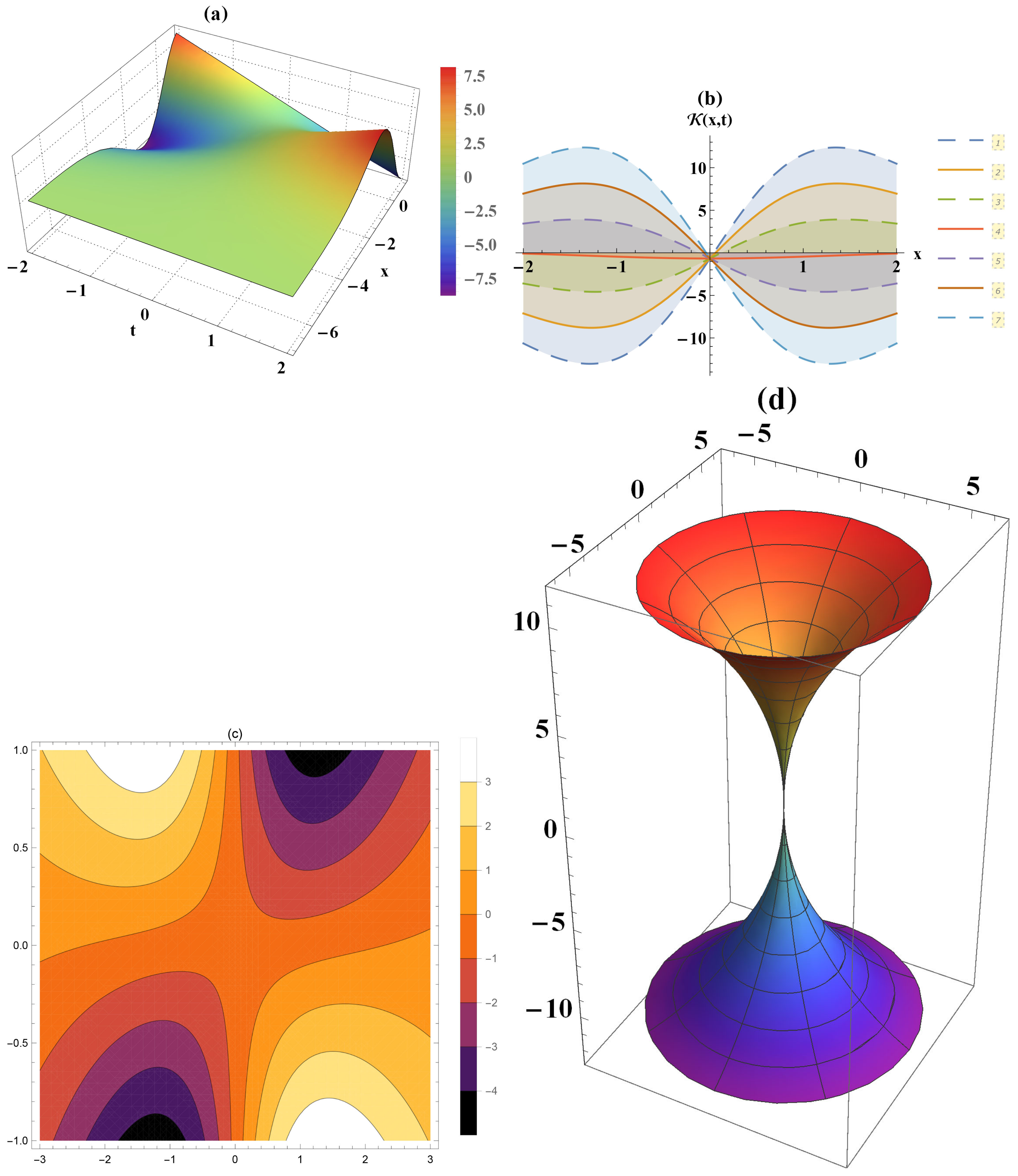
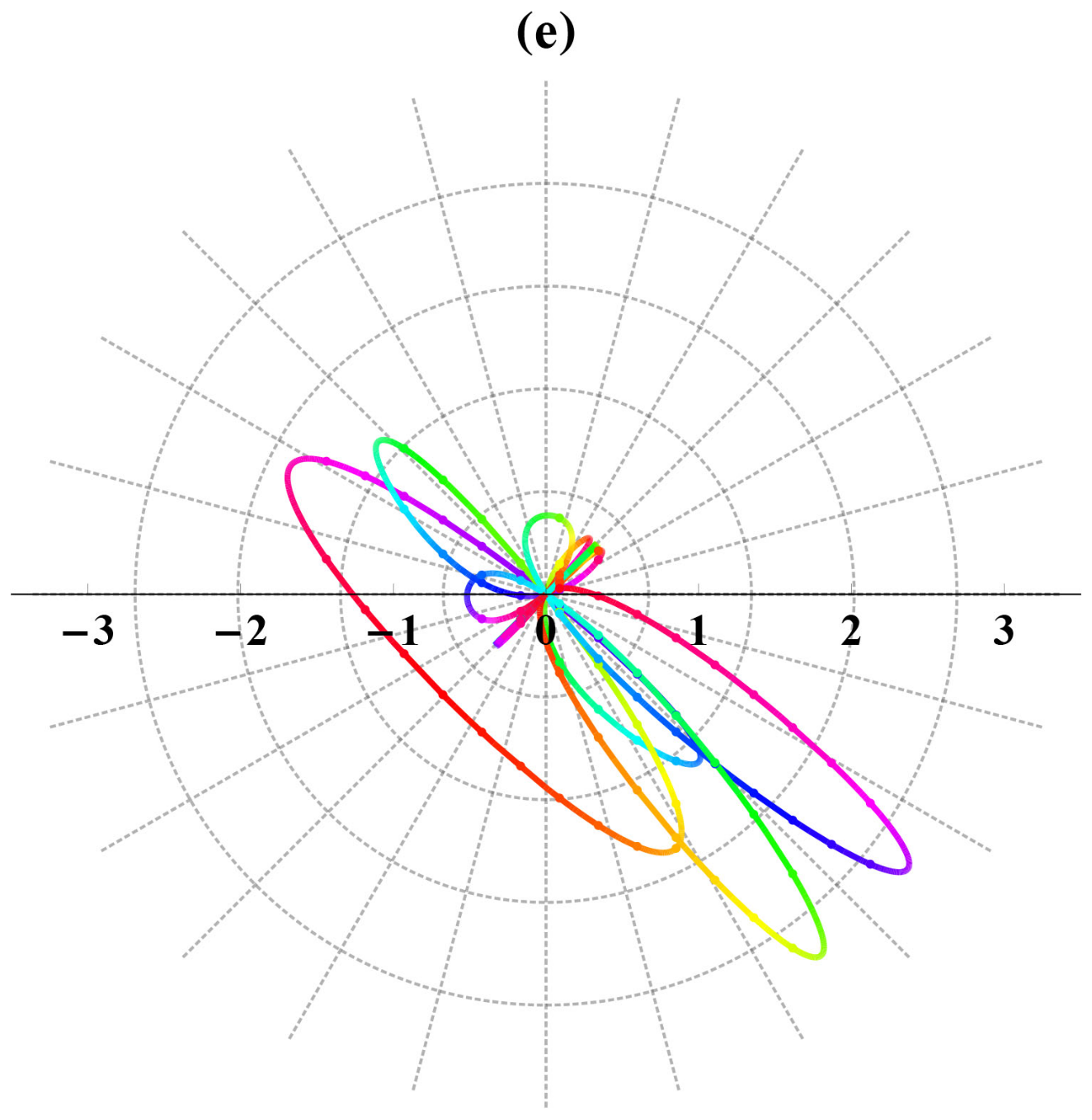
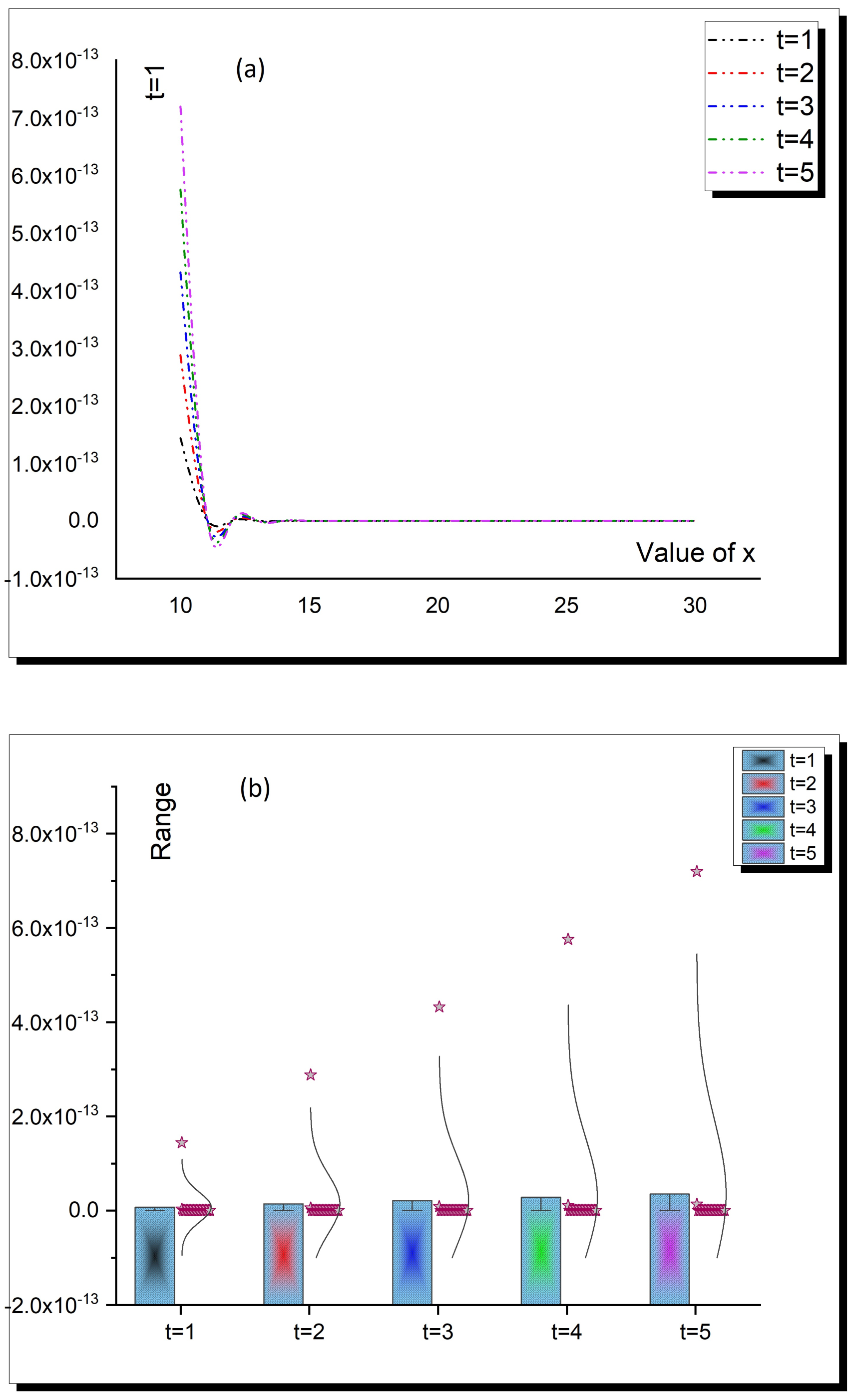
3. Results’ Discussion

Here, the article’s results are illustrated by comparing them with previously published solutions. In contrast, the paper’s contribution is also explained by showing the result’s novelty and shown figures and tables. Additionally, this section shows the obtained solution’s accuracy by estimating the matching between obtained analytical and approximate solutions. The formulated solutions are different from the constructed solutions by numerous researchers who have applied some distinct analytical schemes.
This paper has applied the MFE and NAE analytical schemes to the considered model for constructing novel solutions. Both computational methods depend on the above-shown auxiliary equations that are different from the previous techniques. These auxiliary equations provide some distinct solutions by giving a specific value of parameters. The considered model is studied by utilizing some analytical and numerical schemes such as the homotopy perturbation method (HPM) [26], different methods of fixed-point theorem together with the concept of Piccard L-stability [27], the deep geometric theory of Krasil’shchik and Vinogradov that is known with a nonlocal symmetries theory [28], the q-homotopy analysis transform method (q-HATM) [29], the modified auxiliary equation of direct algebraic method [30], the Adomian decomposition method (ADM) [31], perturbation scheme and the Hirota bi-linear formalism [32]. However, all these are studies of the considered model, but our paper has constructed novel solutions that have not been obtained in previously published articles.
Figure 1, Figure 2, Figure 3, Figure 4, Figure 5 and Figure 6 show the dynamical behavior of the obtained solutions through the pseudo spherical surfaces, respectively, kink, bright, dark, bright, dark, and dark waves. These figures have been plotted by using the following values of the above-shown parameters in its represented solution [ a 2 = 4 ,   a 2 = 2 ,   a 1 = 5 ,   λ = 3 ,   ϱ = 16   &   a 0 = 0.3 ,   a 2 = 0.5 ,   a 2 = 0.1 ,   a 1 = 0.9 ,   λ = 7 ,   q 2 = 0.8 ,   q 4 = 0.4 ,   ϱ = 4   &   a 2 = 5 ,   λ = 7 ,   P 1 = 1 ,   P 2 = 3 ,   P 3 = 2   &   a 2 = 5 ,   λ = 7 ,   P 1 = 1 ,   P 2 = 3 ,   P 3 = 2   &   a 0 = 5 ,   λ = 7 ,   P 1 = 1 ,   P 2 = 3 ,   P 3 = 2 ,   q 2 = 6 ,   q 4 = 8   &   a 0 = 5 ,   λ = 7 ,   P 1 = 1 ,   P 2 = 3 ,   P 3 = 2 ,   q 2 = 6 ,   P 4 = 8 ] . For further explanation of the sketched solutions Equations (4), (6), (14), (16), (22), and (24), three, two-dimensional, contour, polar, and spherical plots have been figured to show more novel properties of the wave’s dynamical behavior on the considered surface.
Estimating the matching between analytical and approximate solutions by using the analytical obtained solutions for constructing the requested conditions allows applying the VI method. The approximate solutions of the considered model are also sketched in distinct forms (Figure 7 and Figure 8). While the matching between the analytical and approximate solutions is discussed through Table 1 and Table 2 and Figure 9 and Figure 10. Additionally, The MFE method’s accurate is greater than the NAE method, and this superiority is explained by Figure 11:

4. Conclusions

This paper has successfully implemented two recent analytical schemes for obtaining novel solutions of the nonlinear KK -model. Many computational wave solutions have been formulated through the used schemes. These solutions have been checked for their accuracy by employing the VI approximate schemes. The solutions have been represented in some different sketches to explain the physical and dynamical characterizations of the waves on pseudo-spherical surfaces. The paper’s novelty and contribution are demonstrated by comparing its solutions with the previously published results of the considered model.

Author Contributions

M.M.A.K. and L.A. have contributted in first draft, software, and methodology, S.K.E. and M.A.E.-S. have contributted in formal analysis and investigation, while S.H.A., J.F.A., and N.A.A. have contributted in writing—review and editing. All authors have read and agreed to the published version of the manuscript.

Funding

This paper has been funded by the deanship of scientific research at the King Khalid University, Abha, KSA, grant number (RGP. 2/121/42), and Taif University researchers supporting project number (TURSP-2020/247), Taif University, Taif, Saudi Arabia.

Data Availability Statement

The data that support the findings of this study are available from the corresponding author upon reasonable request.

Acknowledgments

This Research was supported by the deanship of scientific research at the King Khalid University, Abha, KSA, grant number (RGP. 2/121/42), and Taif University researchers supporting project number (TURSP-2020/247), Taif University, Taif, Saudi Arabia.

Code Availability

The used code of this study is available from the corresponding author upon reasonable request.

Conflicts of Interest

There is no conflict of interest.

References

  1. Wang, K.J. A new fractional nonlinear singular heat conduction model for the human head considering the effect of febrifuge. Eur. Phys. J. Plus 2020, 135, 1–7. [Google Scholar] [CrossRef]
  2. Park, C.; Khater, M.M.; Abdel-Aty, A.H.; Attia, R.A.; Rezazadeh, H.; Zidan, A.; Mohamed, A.B. Dynamical analysis of the nonlinear complex fractional emerging telecommunication model with higher–order dispersive cubic–quintic. Alex. Eng. J. 2020, 59, 1425–1433. [Google Scholar] [CrossRef]
  3. Gao, W.; Rezazadeh, H.; Pinar, Z.; Baskonus, H.M.; Sarwar, S.; Yel, G. Novel explicit solutions for the nonlinear Zoomeron equation by using newly extended direct algebraic technique. Opt. Quantum Electron. 2020, 52, 1–13. [Google Scholar] [CrossRef]
  4. Khater, M.M. Comment on four papers of Elsayed ME Zayed, Abdul-Ghani Al-Nowehy, Reham MA Shohib and Khaled AE Alurrfi (Optik 130 (2017) 1295–1311 & Optik 143 (2017) 84–103 & Optik 158 (2018) 970–984 & optik 144 (2017) 132–148). Optik 2018, 172, 585–587. [Google Scholar] [CrossRef]
  5. Khater, M.M.; Hamed, Y.S.; Lu, D. On rigorous computational and numerical solutions for the voltages of the electrified transmission range with the day yet distance. Numer. Methods Partial. Differ. Equ. 2020, 1–10. [Google Scholar] [CrossRef]
  6. Khater, M.M.; Mousa, A.; El-Shorbagy, M.; Attia, R.A. Analytical and semi-analytical solutions for Phi-four equation through three recent schemes. Results Phys. 2021, 22, 103954. [Google Scholar] [CrossRef]
  7. Khater, M.M.; Ahmed, A.E.S.; El-Shorbagy, M. Abundant stable computational solutions of Atangana–Baleanu fractional nonlinear HIV-1 infection of CD4+ T–cells of immunodeficiency syndrome. Results Phys. 2021, 22, 103890. [Google Scholar] [CrossRef]
  8. Khater, M.M. Diverse solitary and Jacobian solutions in a continually laminated fluid with respect to shear flows through the Ostrovsky equation. Mod. Phys. Lett. B 2021, 35, 2150220. [Google Scholar] [CrossRef]
  9. Khater, M.M.; Anwar, S.; Tariq, K.U.; Mohamed, M.S. Some optical soliton solutions to the perturbed nonlinear Schrödinger equation by modified Khater method. AIP Adv. 2021, 11, 025130. [Google Scholar] [CrossRef]
  10. Khater, M.M.; Attia, R.A.; Bekir, A.; Lu, D. Optical soliton structure of the sub-10-fs-pulse propagation model. J. Opt. 2021, 50, 109–119. [Google Scholar] [CrossRef]
  11. Chu, Y.; Khater, M.M.; Hamed, Y. Diverse novel analytical and semi-analytical wave solutions of the generalized (2+1)-dimensional shallow water waves model. AIP Adv. 2021, 11, 015223. [Google Scholar] [CrossRef]
  12. Attia, R.A.; Baleanu, D.; Lu, D.; Khater, M.M.; Ahmed, E.S. Computational and numerical simulations for the deoxyribonucleic acid (DNA) model. Discret. Contin. Dyn. Syst. S 2021. [Google Scholar] [CrossRef]
  13. Khater, M.M.; Bekir, A.; Lu, D.; Attia, R.A. Analytical and semi-analytical solutions for time-fractional Cahn–Allen equation. Math. Methods Appl. Sci. 2021, 44, 2682–2691. [Google Scholar] [CrossRef]
  14. Khater, M.M.; Attia, R.A.; Park, C.; Lu, D. On the numerical investigation of the interaction in plasma between (high & low) frequency of (Langmuir & ion-acoustic) waves. Results Phys. 2020, 18, 103317. [Google Scholar]
  15. Khater, M.M.; Baleanu, D. On abundant new solutions of two fractional complex models. Adv. Differ. Equ. 2020, 2020, 1–14. [Google Scholar] [CrossRef]
  16. Khater, M.M.; Attia, R.A.; Lu, D. Computational and numerical simulations for the nonlinear fractional Kolmogorov–Petrovskii–Piskunov (FKPP) equation. Phys. Scr. 2020, 95, 055213. [Google Scholar] [CrossRef]
  17. Li, J.; Attia, R.A.; Khater, M.M.; Lu, D. The new structure of analytical and semi-analytical solutions of the longitudinal plasma wave equation in a magneto-electro-elastic circular rod. Mod. Phys. Lett. B 2020, 34, 2050123. [Google Scholar] [CrossRef]
  18. Khater, M.M.; Attia, R.A.; Alodhaibi, S.S.; Lu, D. Novel soliton waves of two fluid nonlinear evolutions models in the view of computational scheme. Int. J. Mod. Phys. B 2020, 34, 2050096. [Google Scholar] [CrossRef]
  19. Abdel-Aty, A.H.; Khater, M.M.; Baleanu, D.; Khalil, E.; Bouslimi, J.; Omri, M. Abundant distinct types of solutions for the nervous biological fractional FitzHugh–Nagumo equation via three different sorts of schemes. Adv. Differ. Equ. 2020, 2020, 1–17. [Google Scholar] [CrossRef]
  20. Yue, C.; Khater, M.M.; Attia, R.A.; Lu, D. Computational simulations of the couple Boiti–Leon–Pempinelli (BLP) system and the (3+1)-dimensional Kadomtsev–Petviashvili (KP) equation. AIP Adv. 2020, 10, 045216. [Google Scholar] [CrossRef] [Green Version]
  21. Yue, C.; Khater, M.M.; Inc, M.; Attia, R.A.; Lu, D. Abundant analytical solutions of the fractional nonlinear (2+1)-dimensional BLMP equation arising in incompressible fluid. Int. J. Mod. Phys. B 2020, 34, 2050084. [Google Scholar] [CrossRef]
  22. Khater, M.M.; Park, C.; Lu, D. Two effective computational schemes for a prototype of an excitable system. AIP Adv. 2020, 10, 105120. [Google Scholar] [CrossRef]
  23. Abdel-Aty, A.H.; Khater, M.M.; Baleanu, D.; Abo-Dahab, S.; Bouslimi, J.; Omri, M. Oblique explicit wave solutions of the fractional biological population (BP) and equal width (EW) models. Adv. Differ. Equ. 2020, 2020, 1–17. [Google Scholar] [CrossRef]
  24. Khater, M.M.; Mohamed, M.S.; Attia, R.A. On semi analytical and numerical simulations for a mathematical biological model; the time-fractional nonlinear Kolmogorov–Petrovskii–Piskunov (KPP) equation. Chaos Solitons Fractals 2021, 144, 110676. [Google Scholar] [CrossRef]
  25. Khater, M.M.; Inc, M.; Nisar, K.; Attia, R.A. Multi–solitons, lumps, and breath solutions of the water wave propagation with surface tension via four recent computational schemes. Ain Shams Eng. J. 2021. [Google Scholar] [CrossRef]
  26. Mohyud-Din, S.T.; Yıldırım, A.; Sarıaydın, S. Numerical soliton solution of the Kaup-Kupershmidt equation. Int. J. Numer. Methods Heat Fluid Flow 2011. [Google Scholar] [CrossRef]
  27. Atangana, A.; Goufo, E.F.D. Conservatory of Kaup-Kupershmidt equation to the concept of fractional derivative with and without singular kernel. Acta Math. Appl. Sin. Engl. Ser. 2018, 34, 351–361. [Google Scholar] [CrossRef]
  28. Reyes, E.G. Nonlocal symmetries and the Kaup–Kupershmidt equation. J. Math. Phys. 2005, 46, 073507. [Google Scholar] [CrossRef]
  29. Prakasha, D.G.; Malagi, N.S.; Veeresha, P.; Prasannakumara, B.C. An efficient computational technique for time-fractional Kaup-Kupershmidt equation. Numer. Methods Partial Differ. Equ. 2021, 37, 1299–1316. [Google Scholar] [CrossRef]
  30. Aljahdaly, N.H.; Seadawy, A.R.; Albarakati, W.A. Applications of dispersive analytical wave solutions of nonlinear seventh order Lax and Kaup-Kupershmidt dynamical wave equations. Results Phys. 2019, 14, 102372. [Google Scholar] [CrossRef]
  31. Inç, M. On numerical soliton solution of the Kaup–Kupershmidt equation and convergence analysis of the decomposition method. Appl. Math. Comput. 2006, 172, 72–85. [Google Scholar]
  32. Musette, M.; Verhoeven, C. Nonlinear superposition formula for the Kaup–Kupershmidt partial differential equation. Phys. D Nonlinear Phenom. 2000, 144, 211–220. [Google Scholar] [CrossRef]
Figure 1. Distinct kink waves’ sketches of Equation (4) in various formulas (three (a), two (b), contour (c), spherical (d), polar plots (e)) for a 2 = 4 ,   a 2 = 2 ,   a 1 = 5 ,   λ = 3 ,   ϱ = 16 .
Symmetry 13 00963 g001aSymmetry 13 00963 g001b
Figure 2. Distinct bright waves’ sketches of Equation (6) in various formulas (three (a), two (b), contour (c), spherical (d), polar plots (e)) for a 0 = 0.3 ,   a 2 = 0.5 ,   a 2 = 0.1 ,   a 1 = 0.9 ,   λ = 7 ,   q 2 = 0.8 ,   q 4 = 0.4 ,   ϱ = 4 .
Symmetry 13 00963 g002aSymmetry 13 00963 g002b
Figure 3. Distinct dark waves’ sketches of Equation (14) in various formulas (three (a), two (b), contour (c), spherical (d), polar plots (e)) for a 2 = 5 ,   λ = 7 ,   P 1 = 1 ,   P 2 = 3 ,   P 3 = 2 .
Symmetry 13 00963 g003
Figure 4. Distinct bright waves’ sketches of Equation (22) in various formulas (three (a), two (b), contour (c), spherical (d), polar plots (e) for a 2 = 5 ,   λ = 7 ,   P 1 = 1 ,   P 2 = 3 ,   P 3 = 2 .
Symmetry 13 00963 g004
Figure 5. Distinct dark waves’ sketches of Equation (16) in various formulas (three (a), two (b), contour (c), spherical (d), polar plots (e)) for a 0 = 5 ,   λ = 7 ,   P 1 = 1 ,   P 2 = 3 ,   P 3 = 2 ,   q 2 = 6 ,   q 4 = 8 .
Symmetry 13 00963 g005aSymmetry 13 00963 g005b
Figure 6. Distinct dark waves’ sketches of Equation (24) in various formulas (three (a), two (b), contour (c), spherical (d), polar plots (e)) for a 0 = 5 ,   λ = 7 ,   P 1 = 1 ,   P 2 = 3 ,   P 3 = 2 ,   q 2 = 6 ,   P 4 = 8 .
Symmetry 13 00963 g006aSymmetry 13 00963 g006b
Figure 7. Distinct bright waves’ sketches of the obtained approximate solution by the calculated data from the MFE method’s solutions in various formulas (three (a), two (b), contour (c), spherical (d), polar plots (e)).
Symmetry 13 00963 g007aSymmetry 13 00963 g007b
Figure 8. Distinct bright waves’ sketches of the obtained approximate solution by the calculated data from the NAE method’s solutions in various formulas (three (a), two (b), contour (c), spherical (d), polar plots (e)).
Symmetry 13 00963 g008aSymmetry 13 00963 g008b
Figure 9. Absolute error through Table 1, through (a) two-dimensional, and (b) bar normal plots.
Symmetry 13 00963 g009
Figure 10. Absolute error through Table 2., through (a) two-dimensional, and (b) distribution plots.
Symmetry 13 00963 g010
Figure 11. Accuracy of the MFE expansion method over NAE method through (a) two-dimensional, and (b) distribution plots.
Symmetry 13 00963 g011
Table 1. Absolute error between analytical and approximate solutions through the MFE and VI methods for x     { 10 , 11 , , 29 , 30 } ,   t { 1 , 2 , 3 , 4 , 5 } .
Value of x t = 1 t = 2 t = 3 t = 4 t = 5
101.4432899320127 × 10−132.88213897192691 × 10−134.32098801184111 × 10−135.75539615965681 × 10−137.19424519957101 × 10⁻¹³
113.10862446895044 × 10−155.77315972805081 × 10−158.43769498715119 × 10−151.11022302462516 × 10−141.37667655053519 × 10⁻¹⁴
124.44089209850063 × 10−164.44089209850063 × 10−164.44089209850063 × 10−164.44089209850063 × 10−164.44089209850063 × 10⁻¹⁶
134.44089209850063 × 10−164.44089209850063 × 10−164.44089209850063 × 10−164.44089209850063 × 10−164.44089209850063 × 10⁻¹⁶
144.44089209850063 × 10−164.44089209850063 × 10−164.44089209850063 × 10−164.44089209850063 × 10−164.44089209850063 × 10⁻¹⁶
154.44089209850063 × 10−164.44089209850063 × 10−164.44089209850063 × 10−164.44089209850063 × 10−164.44089209850063 × 10⁻¹⁶
164.44089209850063 × 10−164.44089209850063 × 10−164.44089209850063 × 10−164.44089209850063 × 10−164.44089209850063 × 10⁻¹⁶
174.44089209850063 × 10−164.44089209850063 × 10−164.44089209850063 × 10−164.44089209850063 × 10−164.44089209850063 × 10⁻¹⁶
184.44089209850063 × 10−164.44089209850063 × 10−164.44089209850063 × 10−164.44089209850063 × 10−164.44089209850063 × 10⁻¹⁶
194.44089209850063 × 10−164.44089209850063 × 10−164.44089209850063 × 10−164.44089209850063 × 10−164.44089209850063 × 10⁻¹⁶
204.44089209850063 × 10−164.44089209850063 × 10−164.44089209850063 × 10−164.44089209850063 × 10−164.44089209850063 × 10⁻¹⁶
214.44089209850063 × 10−164.44089209850063 × 10−164.44089209850063 × 10−164.44089209850063 × 10−164.44089209850063 × 10⁻¹⁶
224.44089209850063 × 10−164.44089209850063 × 10−164.44089209850063 × 10−164.44089209850063 × 10−164.44089209850063 × 10⁻¹⁶
234.44089209850063 × 10−164.44089209850063 × 10−164.44089209850063 × 10−164.44089209850063 × 10−164.44089209850063 × 10⁻¹⁶
244.44089209850063 × 10−164.44089209850063 × 10−164.44089209850063 × 10−164.44089209850063 × 10−164.44089209850063 × 10⁻¹⁶
254.44089209850063 × 10−164.44089209850063 × 10−164.44089209850063 × 10−164.44089209850063 × 10−164.44089209850063 × 10⁻¹⁶
264.44089209850063 × 10−164.44089209850063 × 10−164.44089209850063 × 10−164.44089209850063 × 10−164.44089209850063 × 10⁻¹⁶
274.44089209850063 × 10−164.44089209850063 × 10−164.44089209850063 × 10−164.44089209850063 × 10−164.44089209850063 × 10⁻¹⁶
284.44089209850063 × 10−164.44089209850063 × 10−164.44089209850063 × 10−164.44089209850063 × 10−164.44089209850063 × 10⁻¹⁶
294.44089209850063 × 10−164.44089209850063 × 10−164.44089209850063 × 10−164.44089209850063 × 10−164.44089209850063 × 10⁻¹⁶
304.44089209850063 × 10−164.44089209850063 × 10−164.44089209850063 × 10−164.44089209850063 × 10−164.44089209850063 × 10⁻¹⁶
Table 2. Absolute error between analytical and approximate solutions through the MFE and VI methods for x { 10 , 11 , , 29 , 30 } ,   t { 5 , 7 , 9 , 11 , 13 } .
Value of xt = 5t = 7t = 9t = 11t = 13
100.01642447253439190.166544416407750.7682910420828990.7642965737157690.15456101130636
110.006125103883911580.06544024008768140.4132941053645880.9918501122666080.41035480239668
120.002264614676074470.02467527923994480.178249014081630.7834494307251060.782908753326303
130.0008346414327102260.00916082072570040.06974670122400050.4188713107954380.998698061991988
140.0003072555799777390.0033814486175110.02625961629628960.1803008542528830.785968774011267
150.0001130611942470330.001245509275063780.009743676386212760.07050154470267170.419798142092268
160.00004159670375103450.0004584064402505250.003595870670760890.02653730954251680.180641818692087
170.00001530308843716850.000168666627386460.001324390934879350.009845834272704360.0706269788158394
185.62976149848238 × 10−60.00006205281824972490.0004874254075307730.003633452490822810.0265834542153602
192.07108297073377 × 10−60.00002282847495571620.0001793421124187680.001338216518425420.00986280995476424
207.61910125712806 × 10−78.39819683040588 × 10−60.00006598011020020330.0004925115560998620.00363969749601051
212.80291244492137 × 10−73.08953346023211 × 10−60.00002427324498915920.0001812132019959890.00134051392754658
221.03113409810618 × 10−71.13657712896842 × 10−68.92969803173438 × 10−60.00006666844559966020.000493356725697391
233.79333067179743 × 10−84.18123533130199 × 10−73.28506182639687 × 10−60.00002452646943273960.000181524122517152
241.39548841371351 × 10−81.53819075254802 × 10−71.20850799517624 × 10−69.02285409870585 × 10−60.0000667828268674509
255.13371495314274 × 10−95.6586878571796 × 10−84.44585419978605 × 10−73.31933202823986 × 10−60.0000245685479496327
261.88858823024773 × 10−92.08171497262377 × 10−81.63553859455767 × 10−71.22111529793356 × 10−69.03833392007503 × 10⁻⁶
276.94772794851417 × 10−107.65820140635753 × 10−96.01681055534264 × 10−84.49223387488651 × 10−73.32502673627832 × 10−6
282.5559265814934 × 10−102.81729489737259 × 10−92.21346095341524 × 10−81.65260072348961 × 10−71.22321026396754 × 10−6
299.40272304461587 × 10−111.03642483484379 × 10−98.14286776895656 × 10−96.0795786183121 × 10−84.49994082385441 × 10−7
303.45907191778849 × 10−113.81279452454919 × 10−102.99559366201407 × 10−92.23655203246409 × 10−81.65543595165296 × 10⁻⁷
Publisher’s Note: MDPI stays neutral with regard to jurisdictional claims in published maps and institutional affiliations.

