Article

Identifying the Locations of Atmospheric Pollution Point Source by Using a Hybrid Particle Swarm Optimization

by
Wipawinee Chaiwino
1,2,
Panasun Manorot
1,2,
Kanyuta Poochinapan
2,3,4 and
Thanasak Mouktonglang
2,3,4,*
1
Ph.D. Degree Program in Faculty of Science, Chiang Mai University, Chiang Mai 50200, Thailand
2
Department of Mathematics, Faculty of Science, Chiang Mai University, Chiang Mai 50200, Thailand
3
Advanced Research Center for Computational Simulation, Chiang Mai University, Chiang Mai 50200, Thailand
4
Centre of Excellence in Mathematics, CHE, Si Ayutthaya Rd., Bangkok 10400, Thailand
*
Author to whom correspondence should be addressed.
Submission received: 28 April 2021 / Revised: 26 May 2021 / Accepted: 28 May 2021 / Published: 1 June 2021
(This article belongs to the Special Issue Modelling and Simulation of Natural Phenomena of Current Interest)

Abstract

:
This research aims to improve the particle swarm optimization (PSO) algorithm by combining a multidimensional search with a line search to determine the location of the air pollution point sources and their respective emission rates. Both multidimensional search and line search do not require the derivative of the cost function. By exploring a symmetric property of search domain, this innovative search tool incorporating a multidimensional search and line search in the PSO is referred to as the hybrid PSO (HPSO). Measuring the pollutant concentration emanating from the pollution point sources through the aid of sensors represents the first stage in the process of evaluating the efficiency of HPSO. The summation of the square of the differences between the observed concentration and the concentration that is theoretically expected (inverse Gaussian plume model or numerical estimations) is used as a cost function. All experiments in this research are therefore conducted using the HPSO sensing technique. To effectively identify air pollution point sources as well as calculate emission rates, optimum positioning of sensors must also be determined. Moreover, the frame of discussion of this research also involves a detailed comparison of the results obtained by the PSO algorithm, the GA (genetic algorithm) and the HPSO algorithm in terms of single pollutant location detection, respectively. In the case of multiple sources, only the findings based on PSO and HPSO algorithms are taken into consideration. This research eventually verifies and confirms that the HPSO does offer substantially better performance in the measuring of pollutant locations as well as emission rates of the air pollution point sources than the original PSO.

1. Introduction

With the rapid growth of industrial and agricultural activities in the developing countries, the industrial and agricultural economic sectors are becoming the primary and secondary sectors that play a major role in countries’ GDP. While the process of product manufacturing triggers the releases of pollutants into the atmosphere within a reasonable threshold, there are times when some industrial plants or farming activities illegally release pollutants into the air well beyond this threshold. During the harvest season, some farmers burn their fields after the harvesting to prepare for the next crops instead of using alternatives such as burying the stubble or residues back into the ground. Burning the fields is the fastest way to clean up the fields and it is followed by selling their products such as local wild vegetables. This contributes to a gradual increase in the practice of illegal land burning. The toxic fumes that emanate from industrial plants and this field burning practice have been identified as the main cause of air pollution, which affects the daily life and the health of people, especially in areas that are surrounded by mountains. This issue faced by the local population has led some researchers to try to monitor the concentration of air pollution more accurately to inform those concerned [1,2,3].
However, if we want to be effective in our fight against pollution, we must first, eradicate the roots of the problem instead of just treating the symptoms. This means being able to identify the atmospheric pollution sources and their corresponding characteristics. This data can be used by the local authorities for issuing factories or farms with an initial warning while allowing an in-depth investigation of the real-time causes and sources of the detected pollution. Hence, there are many researchers who are interested in this topic and who have started improving some algorithms or models that can efficiently and effectively specify the exact positions of pollution sources [4,5,6,7,8]. The problem of identification of the pollution sources is reformulated into a highly nonlinear optimization. Heuristic optimization methods, such as Genetic Algorithm (GA) and Particle Swarm Optimization (PSO), have been applied to solve this class of problems. A genetic algorithm is another empirical search motivated by Charles Darwin’s theory of evolution [9,10,11]. The algorithm imitates the procedure of natural selection where the fittest population are selected for reproduction and produce the offspring which are the next generation. The algorithm produces offspring which inherit the characteristic of their parents which will be a better generation. This simple idea can be applied for searching for the best solution. There are five important phases in GA which are initial population, fitness function, selection, crossover and mutation. In 2013, Quan-min BU [5] proposed an improved genetic algorithm for searching for pollution sources. Like GA, particle swarm optimization is another popular heuristic optimization method. Indeed, PSO is based on the social behavior or large groups, such as flying flocks of birds or fish schools. The moving direction and velocity of the particles are calculated based upon their experience together with social interaction with other particles in the swarm. The social interaction parameter such as cognitive, social and inertia parameters are also introduced in the model.
There are comparative results between the performance of GA and PSO [12,13]. Both methods are very popular mainly because of the implementation and the capability to solve complex problems, e.g., [14,15,16,17,18]. The disadvantage of the GA is that it has high implementation cost and usually requires a higher number of iterations and high number of elements. In particular, in this situation, the cost of each iteration is very high. Furthermore, GA usually converges towards a local optimum rather than the global optimum of the problem, while PSO tries to find the global optima because of their social interaction parameters.
More recently, to achieve effective methods for pollution management and satisfactory emergency responses, there have been many results concerning improving the estimation accuracy concerning airborne pollutant emission source information. In [19], Lang, J. proposed an inversion model which combines the hybrid particle swarm optimization and the Nelder–Mead simplex search method (PSO-NM) with the Gaussian dispersion model to identify the source and to examine the impacts of different atmospheric conditions on the identifications. In the same year [20] Li. H. employed the PSO-NM based on Gaussian puff dispersion model on a three-dimensional neighborhood topology which improves the performance of the PSO. More recently, Albani, R.A.S. [21] proposed an algorithm combining accurate dispersion models, Tikhonov regularization and gradient-descent optimization techniques estimating pollutant emission sources. Moreover, identifying the multiple sources of air pollution locations has also been studied [22,23].
In this research, the focus is to identify a location of air pollution point source both with and without emission rates by using a hybrid PSO (HPSO) on a Gaussian Plume model and a numerical scheme for PDE. Indeed, this paper attempts to apply HPSO to optimize an inverse model based on a numerical scheme of PDE. The HPSO algorithm is a computational technique obtained by improving PSO. We modify the PSO algorithm in two different ways. For the single-point source, the PSO method was first adjusted by adding a multidimensional search. This method is known as the cyclic coordinate method. Besides, a step resembling a mutation from a genetic algorithm (GA) was introduced to identify the locations in two-point sources. Moreover, sensor placement was also designed to increase search efficiency. Finally, we apply the proposed method together with the numerical method for solving PDE. With the numerical scheme, we will be able to apply HPSO to a more complicated PDE model. This research is divided and presented as four main sections. A brief description of the basics of the PSO algorithm, GA, dichotomous search and cyclic coordinate methods constitute the first frame of discussion. Next, we demonstrate how to apply the HPSO to find the atmospheric pollution point sources. The results of this study and the appropriate parameters c 1 , c 2 , ω are discussed in the final part where the single point source without determining the emission rate results are compared with three algorithms consisting of HPSO, PSO and GA. It must be noted that, in the other cases, only the results gained from the original PSO and HPSO are explained.

2. Preliminaries

2.1. Introduction to Particle Swarm Optimization (PSO)

In 1995, the robust evolutionary optimization algorithm inspired by the behavior of organisms such as a flock of birds and fish schools was presented by R. Eberhart and J. Kennedy [24]. It introduced another approach to solving a nonlinear optimization. For the PSO system, an individual particle is a feasible solution in a search space looking for a globally optimal solution. The moving direction and velocity of the particles are calculated based upon their experience together with social interaction with other particles in the swarm. The social interaction parameter such as cognitive, social and inertia parameters are also introduced in the model. PSO is a computational technique using individual improvement gathering with population competition to evaluate the solutions. The algorithm is based on the simulation of the simple social behavior of some animals. In PSO, the term particle is used instead of a feasible solution, a cell swarm instead of a subset of a feasible solution and fitness function instead of an objective function. The particle adjusts its trajectory toward its own previous best position and the previous best position attained by any member of its neighborhood. The fitness function is used for deciding which particle will survive or be eliminated. The locations of all particles are shifted by the velocity equations as below.
V i n + 1 = ω V i n + c 1 r 1 n ( Xlbest i n X i n ) + c 2 r 2 n ( Xgbest n X i n )
X i n + 1 = X i n + V i n + 1
where
P is the swarm’s size.
ω is the inertia weight.
c 1 and c 2 are two positive constants, which are called cognitive and social parameter, respectively.
r 1 n and r 2 n are two random numbers uniformly distributed within range [ 0 , 1 ] .
X i n = x i 1 n , x i 2 n , , x i D n T is the i-th particle of the D-dimensional in n-th iteration.
X l b e s t i n = x l b e s t i 1 n , x l b e s t i 2 n , , x l b e s t i D n T is the best previous position of i-th particle in n-th iteration.
X g b e s t n = x g b e s t 1 n , x g b e s t 2 n , , x g b e s t D n T is the best position of the swarm in n-th iteration.
V i n = v i 1 n , v i 2 n , , v i D n T is velocity of i-th particle in n iteration.  
In Equation (1), ω V i n is the previous particle’s velocity weighted by the inertia weight ω . X l b e s t i n X i n is the direction vector from the i-th particle to the best of the known i-th particle. The direction vector ( X g b e s t i n X i n ) is from the i-th particle to the best know particle. The parameters c 1 and c 2 are the size controller of vectors in the second and the third term, respectively. For more development on PSO and HPSO, see examples in [24,25,26,27,28]. The particle movement and a flowchart of the PSO algorithm are presented Figure 1 and Figure 2. Different versions of modified PSOs have also been proposed to solve different types of non-linear optimization problems. See [29,30,31,32] for examples and more details.

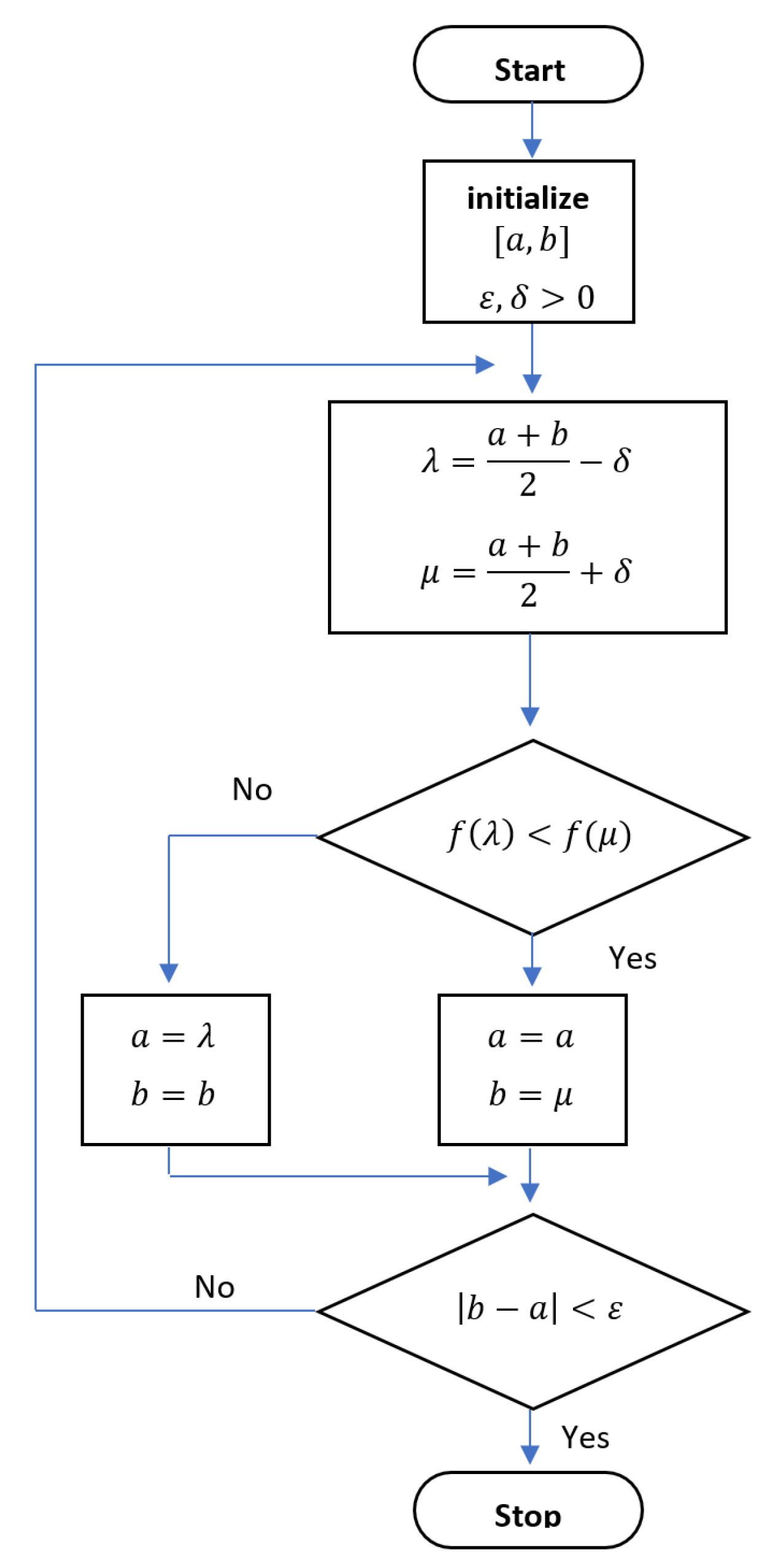
2.2. Dichotomous Search Method

The dichotomous search also known as line search is the searching tool in one dimension for solving a non-linear programming problem. Consider the function f : R R to be minimized over the interval [ a , b ] . First, we pick a small number ε > 0 . Then, according to the flowchart Figure 3, the Dichotomous search involves two steps as follows.
Initialization step: Choose the small constant 2 ε > 0 and the final length of δ > 0 . Let [ a 1 , b 1 ] be the uncertain initial interval. Give k = 1 and then go to main step.
Main step:
  • Consider λ k and μ k given below.
    λ k = a k + b k 2 ε μ k = a k + b k 2 + ε
  • If f ( λ k ) < f ( μ k ) then a k + 1 = a k and b k + 1 = μ k . Otherwise, let a k + 1 = λ k and b k + 1 = b k .
  • If b k a k < δ , stop. Give k = k + 1 and do step 1.

2.3. Cyclic Coordinate Method

The cyclic coordinate method is the multidimensional search without the assistant of the derivative. The objective function f : R n R is the minimized form feasible solution x along the suitable direction d by the Dichotomous search technique. More specifically, we define the feasible solution
x = [ x 1 , x 2 , . . . , x n ] T
to be an n dimensional vector and let the d = [ d 1 , d 2 , . . . , d n ] T be a zero vector in n dimensions except for a 1 at the position that we are investigating. Therefore, the variable x i is updated by x i + d i , while the other variables are kept fixed. The summary below of this method for minimizing the objective function f of multi-variables and a flowchart (Figure 4) are illustrated.
Initialization step: Select a scalar ε > 0 to be used for terminating the method. Let d = [ d 1 , d 2 , . . . , d n ] be the searching small direction and choose the initial point x 1 . Before going to the main step we have to substitute x 1 for y 1 and let k = j = 1 .
Main step:
  • Begin with finding the optimal solution λ from minimizing the problem
    f ( y j + λ d j ) subject   to   λ R
    and then let y j + 1 = y j + λ
  • If j < n , replace j by j + 1 and repeat step 1. Otherwise, if j = n , go to step 3.
  • Let x k + 1 = y n + 1 . If x k + 1 x k < ε , then stop. Otherwise, give y 1 = x k + 1 and j = 1 , surrogate k by k + 1 and go to step 1.

3. Methodology

3.1. Hybrid Particle Swarm Optimization Method (HPSO)

Our hybrid PSO is inspired by a Genetic algorithm (GA) by which each particle can be randomly mutated or evaluated to get to a new region of search domains. For that reason, we incorporate the dichotomous search and the cyclic coordinate search into our PSO. Furthermore, in order to avoid being stuck in some local optimal, we introduce additional procedure to look for another possible local optimal; the procedure is explained as follows.

3.1.1. Optimization Problem Formulation

We begin with providing definitions of the variables in a particle. A particle represents a location of all n contamination point sources (m) and their emission rates (kg/s). Therefore, the i-th particle
X i = ( x i , y i , H i , Q i )
where
x i = [ x i 1 , x i 2 , . . . , x i n ] y i = [ y i 1 , y i 2 , . . . , y i n ] H i = [ h i 1 , h i 2 , . . . , h i n ] Q i = [ q i 1 , q i 2 , . . . , q i n ]
when q i j is the emission rate corresponding the pollution source jth, which is located at ( x i j , y i j , h i j ) of the ith particle. For all i = 1 , 2 , 3 , . . . , p , p is a number of particles (swarm) and n is a number of sources. The fitness function is defined to be a summation of difference between measured and approximated concentration square. In this experiment, we used the Gaussian Plume model for simplicity. Therefore, the approximated concentration C T is the summation of concentration from n different pollution sources. Note that we could use other techniques of approximation in the experiment. C T x i , y i ; H i , Q i is in kg/m 3 from the Gaussian Plume model, which is defined by
F x i , y i ; H i , Q i = i = 1 s μ i C T x i , y i ; H i , Q i 2 , where s is the number of sensor .
where
C T x , y ; H , Q = j = 1 n C x ¯ , y ¯ , z ; H , Q ,
with
C x ¯ , y ¯ , z ; H , Q , = Q 4 π u r y r z e y 4 r y e z H 2 4 r z + e z + H 2 4 r z
x ¯ = x s x , y ¯ = y s y are the shifted coordinates, so the position of source corresponds to ( 0 , 0 , H i ) and
r y x = 1 u 0 x K y ξ d ξ r z x = 1 u 0 x K z ξ d ξ
where u is wind velocity ( m / s ) , K y and K z are diffusion coefficients of y and z directions, respectively [22]. This close form can be used under the ensuing assumptions.
The foul gas is discharged at a constant rate Q (kg/s) form the source x = ( 0 , 0 , H ) , which is placed at height H above the ground surface.
The wind velocity is constant and aligns in the x-axis direction, which is written as u = ( u , 0 , 0 ) when u [ 0 , 5 ] has a unit of m/s.
The solution is in steady state, which makes the wind velocity and other functions independent of time.

The HPSO for Identifying the Single Air Pollution Location and Its Emission Rate

We start with ranking the fitness value of all particles. The first two particles X 1 and X 2 are selected in order to create a new particle by finding the midpoint of the two particles. The middle point is taken as a starting point in the search along the direction d, where d is X 1 X 2 X 1 X 2 . Then go to a selection step; we evaluate the fitness cost of the new particle and select the particles equal to the number of a swarm by ranking the fitness value. Which particle has the most fitness value will be eliminated.

The HPSO for Identifying the Two Air Pollution Locations and Their Emission Rates

For the case of two pollutant sources, we specify just the locations of the source. We adapt the original PSO with the step as follows. In the first step, we rank the fitness cost of each particle and choose the first two particles to create the new particle by the steps below.
Let the first two particles be X 1 = [ x 1 1 , x 1 2 , y 1 1 , y 1 2 ] T and X 2 = [ x 2 1 , x 2 2 , y 2 1 , y 2 2 ] T . The new particle X n e w is with the new random parameter α [ 0 , 100 ] where
( x n e w 1 , y n e w 1 ) = α ( x 1 1 + x 2 1 , y 1 1 + y 2 1 ) 2 ( x n e w 2 , y n e w 2 ) = α ( x 1 2 + x 2 2 , y 1 2 + y 2 2 ) 2 X n e w = [ x n e w 1 , x n e w 2 , y n e w 1 , y n e w 2 ] T
After obtaining the new particles, the particle that provides the worst fitness value is removed. The improved structure of the PSO algorithm is indicated as the following Algorithm 1.
Algorithm 1. HPSO algorithm.
1:
Initailize X i , V i and X l b e s t i for each particle i
2:
while (not termination condition)
3:
for each particle i
4:
Evaluate objective function;
5:
Update X l b e s t i and X g b e s t
6:
end for.
7:
for each i
8:
calculate V i ;
9:
update X i = X i + V i ;
10:
Evaluate objective function;
11:
Choose the first two best particles to create two new particles
12:
Creating a new particle
13:
Evaluate objective function of two new particle and choose the
14:
next generation of the particles
15:
end for
16:
end while

4. Numerical Results

The experiments are designed to investigate the ability of the HPSO algorithm; they are separated into two main parts compose of two-dimensional and three-dimensional domain problems. The results of the identification of the air pollution point source location and its corresponding emission rate are also presented and discussed in two and three-dimension problems. Furthermore, we not only identify the single air pollution point source location but also determine the locations of two-point sources in the two-dimensional domain. For two-point sources, the experiments are designed into two cases. One is to identify the locations of two sources when positioning the source locations beside each other and the other is to identify the locations of two sources when placing source locations in overlapping positions. In the original PSO the parameters c 1 , c 2 and ω play an important role in searching for the optimal solution. This means the relevant c 1 and c 2 help the particles keep a balance among the X l b e s t , X g b e s t and V directions to find the optimal solution. Besides, the appropriate ω increases a chance to find the optimal solution (reduce the change to stick at the local optimal). Therefore, the value ω and c ( c = c 1 = c 2 ) are determined for each experiment. For some problems, there are many values of ω and c that are able to provide the optimal solution. However, the values ω and c produce the best results that are picked; these parameters are searched for in the set { 0.1 , 0.2 , 0.3 , . . . , 1 } and the most appropriate parameters of all experiments are shown in Table 1.
This problem has to do with the identification of the position of atmospheric pollution on the domain size 50,000 m × 35,000 m with light wind (5 m/s). The concentration is emitted with a rate of 35 kg/s by a single pollution point source, which is located at (0, 0) coordinate. For identification of the two-point sources of air pollution, we already mentioned that there are two experiments; the first experiment sources are located at (300, −5000) and (4000, 5000) with emission rates 35 kg/s and 40 kg/s, respectively. In the second experiment, the source locations are moved to (200, 0) and (3000, 0) with the same emission rates.
Firstly, we verify that the number of iterations and the number of particles can reduce the distance error of HPSO by fixing the number of iterations (100 iterations) while the number of particles is increased by 10 from 10 to 250 and by fixing the number of particles (100 particles) while the number of iteration is increased by 10 from 10 to 250. The results are shown in Table 2 and Table 3, respectively. Both sets of results illustrate that, as the number of iterations and particles exceeds 150, the distance error remains homogeneous. In all experiments, mean square error is used to measure the effectiveness of the algorithms.
Next, we point out that, by increasing the number of sensors, the distance error is also reduced. In these experiments, we increase the number of sensors by 2 and observe the results, which are manifested as Table 4.
From Table 4, when the number of sensors is more than two, the distance errors are insignificantly different. So there is good reason to believe that the number of sensors need not be so high. Thus, for all experiments, except two-point sources, in this research we use 100 particles, 200 iterations with four sensors.

4.1. Complexity

In this sub-section, the comparative study of the complexity between the original PSO and our proposed HPSO is discussed. On each iteration of the HPSO, the dichotomous search or the cyclic coordinate method is executed. Let p be the number of particles used in PSO and HPSO. Let also M be the maximum number of iterations for both PSO and HPSO. Then in the original PSO, the number of evaluations of the objective/fitness function is p × M . As for the HPSO, each of the inner iterations for the dichotomous search or the cyclic coordinate method concerning the fitness function has to be evaluated twice. If we assume that the maximum number of the inner iterations is m, then the number of evaluations of the objective/fitness function on our HPSO is 2 p × m × M . It is clear that, on each iteration, the implementation cost of HPSO is higher than PSO. Hence, if the maximum number of iterations is fixed, HPSO takes more computational time. However, the new proposed HPSO is much more effective. To illustrate this point, consider Table 2, where HPSO and PSO are compared for a fixed number of iterations. According to this table, for PSO with 210 particles, the error is about 11.47 m and the computational time is about 4.58 seconds. As for HPSO, there is about the same computational time but with fewer particles—100 particles; the error is only 0.17 m. Hence, even each iteration for HPSO has a higher computation cost above the original PSO; overall, HPSO is considered superior to PSO, especially for situations for which a minimal number of iterations is required.

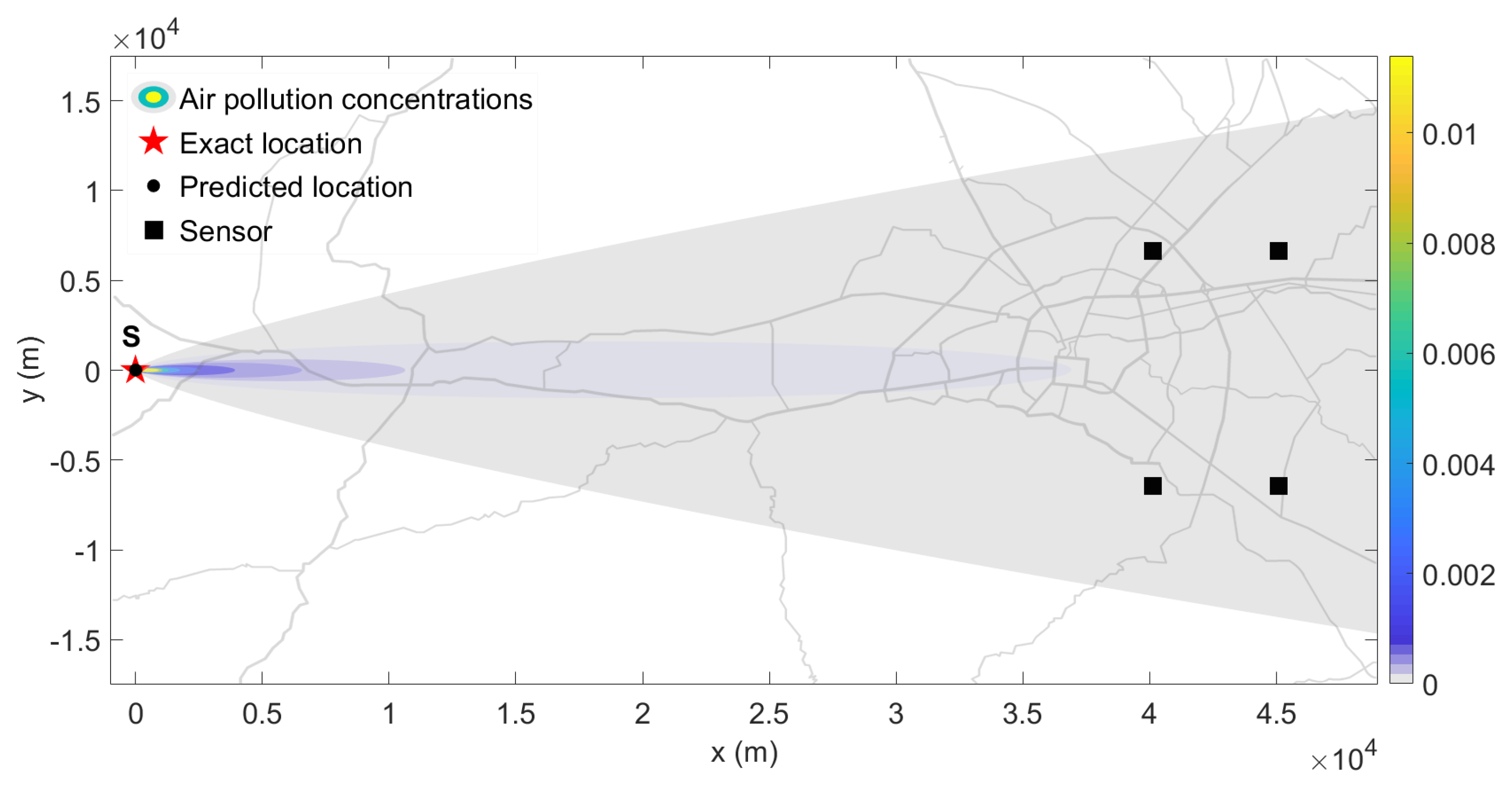
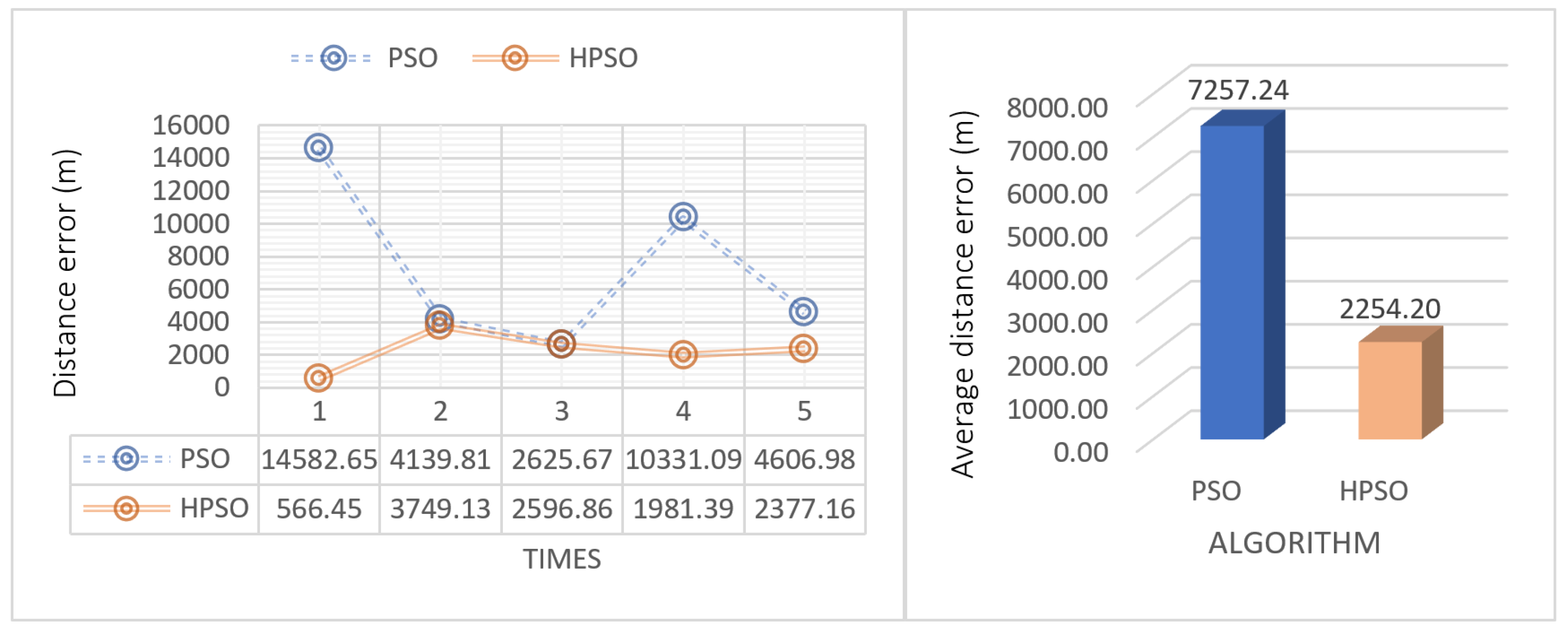
4.2. The Results in Two-Dimensional Domains

The identification of the location of single and multiple air pollution point sources is tested. For comparing the results, the initial data such as the initial particles/chromosomes, the number of particles/chromosomes, the number of sensors and the sensor’s positioning are set to be the same. The results of the three algorithms explicate that the HPSO has the lowest average distance error followed by the original PSO and the original GA. Observe that the HPSO method does not stick at some local optima; consequently, HPSO produces less average distance error than PSO and GA.

4.2.1. Identification the Air Pollution Locations without Finding Emission Rate in Two Dimensions

The results of determining the location of a single air pollution point source are displayed in Figure 5 and Figure 6. The comparative results between GA, PSO and HPSO are illustrated in Figure 5 and Figure 6. Five experiments on each technique were randomly selected and plotted as a line graph on the left and the bar graph on the right displays the average for each technique. As we expect, HPSO outperforms the other techniques. In this experiment, GA has the lowest ability to locate the pollution point source among all three techniques. As for determining the locations of two air pollution point sources, results are displayed as Figure 7, Figure 8, Figure 9 and Figure 10. In these experiments, 300 particles and 500 iterations with four sensors are used for running the program. In both cases of the experiment, the HPSO method processes lower average distance errors than the PSO method. In the first case, the best predicted locations that provide the best average error of the distance errors are ( 332.16 , 5001.74 ) and ( 3784.24 , 4986.78 ) . In the second case, the best predicted locations are ( 320.07 , 208.84 ) and ( 2907.65 , 159.45 ) . Notice that the average distance errors of the HPSO in the case of putting the source location in an overlap of each other is higher than the other case. Note that, for the case of multiple point source, the problem is much more complex than a single point source. The number of point source and emission rates of each point source need to be prescribed. Each point source can have different emission rates.

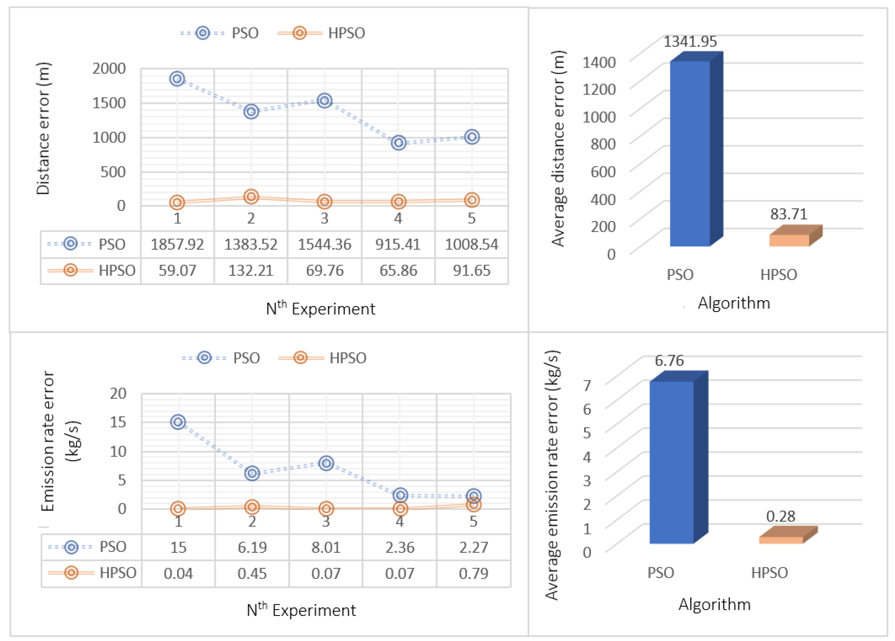
4.2.2. Identification the Air Pollution Locations and Emission Rate in Two Dimensions

Specifying the location together with its corresponding emission rate of the air pollution point source is the last experiment in the two-dimension domain problem. We use 100 particles and 200 iterations to run the program and the results of the PSO method and HPSO method are exhibited as Figure 11 and Figure 12. The HPSO takes an average distance error 16 times less than the PSO and provides an average emission rate error about 24 times lower than the PSO. Hence, we can conclude that our HPSO outperforms PSO. So, we can conclude that our HPSO outperforms the original PSO.

4.3. The Result in Three Dimensional Domains

For the problem in three-dimensional domains, we set the exact source location at (0, 0, 20) on domain size 35,000 m × 50,0000 m × 50 m with the emission rate 35 kg/s. The frame of this problem is divided into two parts which are to identify only the pollution source location and to identify both the location and the emission rate of the pollution source. For the three-dimensional domain experiments, we use 100 particles with 200 iterations.

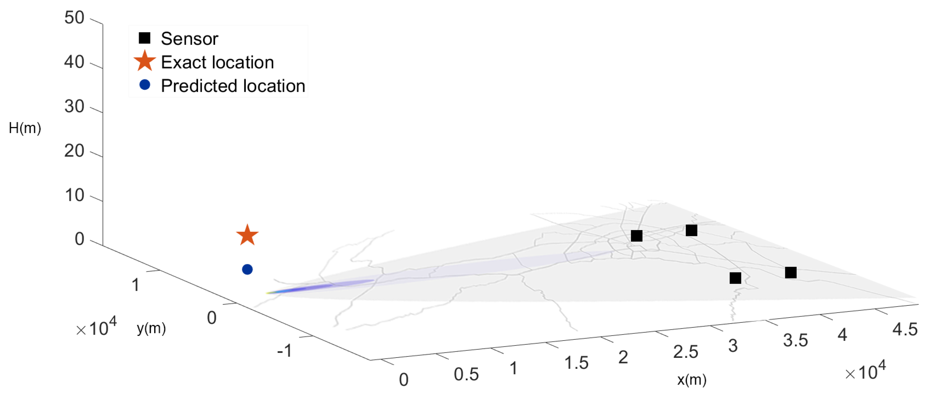
4.3.1. Identification the Air Pollution Locations and Emission Rate in Three Dimensions

Figure 13 and Figure 14 present the result for determining the location of a single-point of the pollutant source and its emission rate. The minimum average error of both items belongs to the HPSO method. Our HPSO outperforms the original PSO.

4.3.2. Identification the Air Pollution Locations without Finding Emission Rate in Three Dimensions

According to Figure 15 and Figure 16, the HPSO algorithm produces an average distance error 29 times less than the PSO algorithm. The HPSO’s computational time is a little bit higher than the PSO’s. In addition, Figure 16 displays the best predicted location of air pollution point source using the HPSO, which is located at ( 0.01 , 0.02 , 20.05 ) .
According to all of the experiments using the Gaussian Plume model, HPSO outperforms PSO. Overall, it is more effective. In order to achieve effective results for pollution management and satisfactory emergency responses, the Gaussian Plume model is not enough. We need to approximate the numerical solution of the set of some governing PDE system. Solving for an estimated solution is very important.

4.4. The Result with a Numerical Method in PDE

In this numerical experiment, we focus on the couple models for pollutant transport, that is, the momentum equations [7,22]:
u t + u u x + v u y = ν 2 u x 2 + 2 u y 2 ,
v t + u v x + v v y = ν 2 v x 2 + 2 v y 2 ,
and the convection–diffusion equation:
C t + u C x + v C y = k 2 C x 2 + 2 C y 2 + S ,
with the following initial-boundary conditions
u ( x , y , 0 ) = u 0 ( x , y ) , v ( x , y , 0 ) = v 0 ( x , y ) , C ( x , y , 0 ) = C 0 ( x , y ) u ( x , y , t ) = f ( x , y , t ) , v ( x , y , t ) = g ( x , y , t ) , C ( x , y , t ) = h ( x , y , t ) , ( x , y ) Ω ,
where u ( x , y , t ) , v ( x , y , t ) are horizontal wind velocity (m/s), C ( x , y , t ) is the concentration of the pollutant (kg/m 3 ), S ( x , , y ) is the source term (kg/m 3 s), ν is kinetic viscosity (m 2 /s) and k ( x , y ) is conductivity (m 2 /s). In this work, we are interested in point-source behaviour. For the n point-source, the source term is given by
S ( x , y ) = i = 1 n Q i δ ( x i , y i ) ( x , y ) ,
where Q i is theemission rate of the i th source and the delta function is defined by
δ ( x i , y i ) ( x , y ) = 1 , if x = x i and y = y i 0 , else .
The conductivity function k ( x , y ) represents the ability according to which the pollutant goes through the median. Thus, the conductivity function depends on the space variables, i.e., the area on the domain. In this study, we assume that the pollutant is emitted in a homogeneous area; that is, the conductivity is constant: k ( x , y ) = k 0 . This assumption can be applied when the source is located in the high area and releases the pollutant to the lower region.

4.4.1. Numerical Method

For the rectangular domain Ω = [ x L , x R ] × [ y L , y R ] , we define the discrete space { ( x i , y j ) | x i = x L + i h x , y j = y L + j h y } , where h x = ( x R x L ) / N x and h y = ( y R y L ) / h y . The temporal domain [ 0 , T ] is discretized as { t n = n τ } , where τ = T / N . Let f i j n = f ( x i , y j , t n ) , the discrete differential operators are given below:
( f i j n ) t ^ = f i j n + 1 f i j n 1 2 τ , ( f i j n ) x = f i + 1 , j n f i j n h x , ( f i j n ) x ¯ = f i j n f i 1 , j n h x ( f i j n ) y = f i , j + 1 n f i j n h y , ( f i j n ) y ¯ = f i j n f i , j 1 n h y , ( f i j n ¯ ) = f i j n + 1 + f i j n 1 2
The numerical scheme for models (4)–(6) is:
( u i j n ) t ^ + u i j n ( u ¯ i j n ) x ^ + v i j n ( u ¯ i j n ) y ^ = ν ( u ¯ i j n ) x x ¯ + u ¯ i j n ) y y ¯
( v i j n ) t ^ + u i j n ( v ¯ i j n ) x ^ + v i j n ( v ¯ i j n ) y ^ = ν ( v ¯ i j n ) x x ¯ + v ¯ i j n ) y y ¯
( C i j n ) t ^ + u i j n ( C ¯ i j n ) x ^ + v i j n ( C ¯ i j n ) y ^ = k ( C ¯ i j n ) x x ¯ + C ¯ i j n ) y y ¯ + S i j n .
The scheme is second order in both time and space.

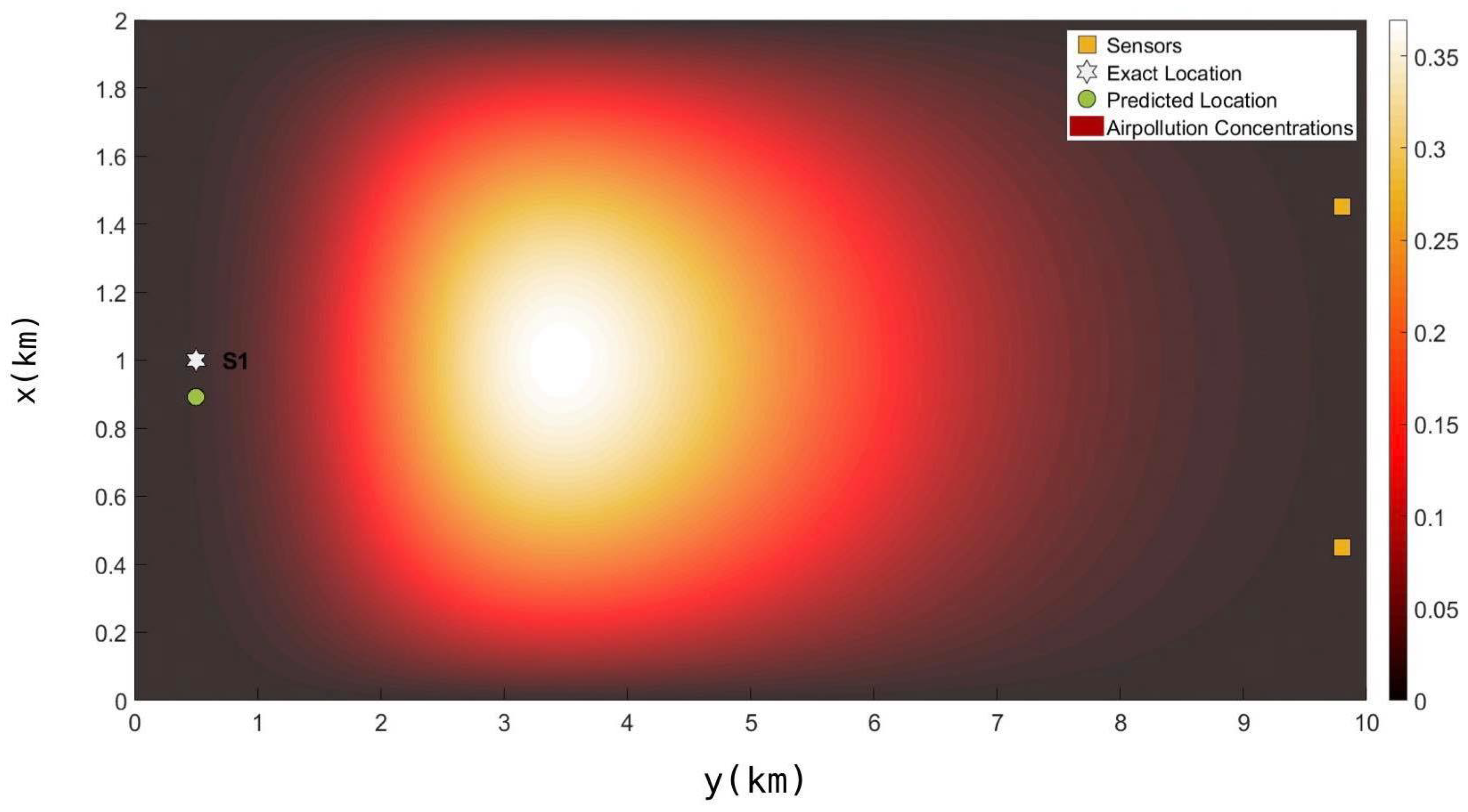
4.4.2. Results of Identifying Single Pollution Point Source

In this experiment, giving an initial guess of the pollution source, we use the above numerical scheme to solve a system of partial differential equations for atmospheric model for concentration on the domain space ( x , y ) . As a result, for each particle on each iteration, solving for the system of PDE is required for evaluating a fitness function. Hence, a fast and accurate numerical method is needed.
Domain size: 10 × 2
The number of particles is 10
The number of iterations is 30
Exact location is (0.5, 1)
We considered three cases for different numbers of time steps. In each case, the program was run five times and then the average error was calculated. The best predicted location is presented in Table 5. According to the results of the experiment, the HPSO is also capable of identifying the location of the point source based on an approximated solution of a system of PDE. The Figure 17, Figure 18 and Figure 19 illustrate how the algorithm identifies the location of the pollution source.

5. Conclusions

This research paper is another comparative study of GA and PSO. Due to the nature of the problems, PSO actually outperforms GA. PSO is able to locate the pollution source more accurately. The results on the Gaussian Plume model are very fascinating. However, in order to apply the optimization techniques to the differential models for pollutant transport, a more effective technique must be used. To evaluate a fitness function for each particle, estimating a solution of a system of PDE is required. In this work, we estimate a solution of a system of partial differential equations for the atmospheric model for concentration on the domain space. It turns out that all of the experiment results explicate that HPSO produces better results than GA and PSO. Besides, HPSO is able to identify the location and its emission rate more accurately when we increase the number of particles and iterations with appropriate parameters ω and c. While the HPSO performs with very high efficiency for specifying the location and its emission rate of single air pollution, in the case of two sources the HPSO gives quite high distance errors. The HPSO is also applicable to a more complicated system. We developed a second order in both space and time numerical schemes for solving pollutant transport equations, system of PDEs. As in the experiment with the numerical method in PDEs, the HPSO method is also able to accurately locate the pollution source. This illustrates that HPSO can be used to optimize the inverse model based on the numerical scheme for PDE. As for future work, a fast numerical scheme for solving PDE could be developed.

Author Contributions

Conceptualization, T.M.; Formal analysis, K.P.; Investigation, W.C. and K.P.; Methodology, W.C. and T.M.; Project administration, T.M.; Software, W.C., P.M. and T.M.; Supervision, T.M.; Writing—original draft, W.C.; Writing—review and editing, K.P. and T.M. All authors have read and agreed to the published version of the manuscript.

Funding

This research is supported by the Centre of Excellence in Mathematics, The Commission on Higher Education, Thailand and by Chiang Mai University, Chiang Mai Thailand.

Institutional Review Board Statement

Not applicable.

Informed Consent Statement

Not applicable.

Data Availability Statement

The data used to support the findings of this study are available from the corresponding author upon request. All the computer codes used in this study are available from the corresponding author upon request.

Acknowledgments

This research was partially supported by the Centre of Excellence in Mathematics, The Commission on Higher Education, Thailand and by Chiang Mai University, Chiang Mai Thailand.

Conflicts of Interest

The authors declare no conflict of interest.

References

  1. Khedo, K.K.; Perseedoss, R.; Mungur, A. A wireless sensor network air pollution monitoring system. arXiv 2010, arXiv:1005.1737. [Google Scholar] [CrossRef]
  2. Hasenfratz, D.; Saukh, O.; Sturzenegger, S.; Thiele, L. Participatory air pollution monitoring using smartphones. Mob. Sens. 2012, 2, 1–5. [Google Scholar]
  3. James, J.Q.; Li, V.O.K.; Lam, A.Y.S. Sensor deployment for air pollution monitoring using public transportation system. In Proceedings of the 2012 IEEE Congress on Evolutionary Computation (CEC), Brisbane, Australia, 10–15 June 2012; pp. 1–7. [Google Scholar]
  4. Cervone, G.; Franzese, P. Non-Darwinian evolution for the source detection of atmospheric releases. Atmos. Environ. 2011, 45, 4497–4506. [Google Scholar] [CrossRef]
  5. Bu, Q.; Wang, Z.; Tong, X. An improved genetic algorithms for searching for pollution sources. Water Sci. Eng. 2013, 6, 392–401. [Google Scholar]
  6. Cantelli, A.; D’orta, F.; Cattini, A.; Sebastianelli, F.; Cedola, L. Application of genetic algorithm for the simultaneous. identification of atmospheric pollution sources. Atmos. Environ. 2015, 115, 36–46. [Google Scholar] [CrossRef]
  7. Sharan, M.; Yadav, A.K.; Singh, M.P.; Agarwal, P.; Nigam, S. A Mathematical Model for the Dispersion of Air Pollutants in Low Wind Conditions. Atmos. Environ. 1996, 30, 1209–1220. [Google Scholar] [CrossRef]
  8. Chaiwino, W.; Mouktonglang, T. Identication of Atmospheric Pollution Source Based on Particle Swarm Optimization. Thai J. Math. 2019, 17, 125–140. [Google Scholar]
  9. Deb, K. An introduction to Genetic Algorithms. Sadhana 1999, 24, 293–315. [Google Scholar] [CrossRef] [Green Version]
  10. Sivanandam, S.N.; Deepa, S.N. Introduction to Genetic Algorithms; Springer Science & Business Media: Berlin/Heidelberg, Germany, 2008. [Google Scholar]
  11. Houck, C.R.; Joines, J.; Kay, M.G. A Genetic Algorithm for Function Optimization: A Matlab Implementation. Ncsu-ie tr 1995, 95, 1–10. [Google Scholar]
  12. Razvan, C. Comparison between the Performance of GA and PSO in Structural Optimization Problems. Am. J. Eng. Res. (AJER) 2016, 5, 268–272. [Google Scholar]
  13. Shahid, S.; Ruchi, S. A Comparative Study of Genetic Algorithm and the Particle Swarm Optimization. Int. J. Electr. Eng. 2016, 9, 215–223. [Google Scholar]
  14. Das, P.K.; Behera, H.S.; Panigrahib, B.K. A hybridization of an Improved Particle Swarm Optimization and Gravitational Search Algorithm for Multi-robot Path Planning. Swarm Evol. Comput. 2016, 28, 14–28. [Google Scholar] [CrossRef]
  15. Fernandes, C.; Pontes, A.J.; Viana, J.C.; Gaspar-Cunha, A. Using multiobjective evolutionary algorithms in the optimization of operating conditions of polymer injection molding. Polym. Eng. Sci. 2010, 50, 1667–1678. [Google Scholar] [CrossRef]
  16. Fernandes, C.; Pontes, A.J.; Viana, J.C.; Gaspar-Cunha, A. Using Multi-objective Evolutionary Algorithms for Optimization of the Cooling System in Polymer Injection Molding. Int. Polym. Process. 2012, 27, 213–223. [Google Scholar] [CrossRef] [Green Version]
  17. Fereshteh, S.; Nima, J. Service Allocation in the Cloud Environments Using Multi-objective Particle Swarm Optimization Algorithm Based on Crowding Distance. Swarm Evol. Comput. 2017, 35, 53–64. [Google Scholar]
  18. Shahid, S.; Ruchi, S. Multi-Objective Optimization of Gate Location and Processing Conditions in Injection Molding Using MOEAs: Experimental Assessment. In Proceedings of the International Conference on Evolutionary Multi-Criterion Optimization (EMO 2015), Guimarães, Portugal, 29 March–1 April 2015; pp. 373–387. [Google Scholar]
  19. Cui, J.; Lang, J.; Chen, T.; Cheng, S.; Shen, Z.; Mao, S. Investigating the Impacts of Atmospheric Diffusion Conditions on Source Parameter Identification based on an Optimized Inverse Modelling Method. Atmos. Environ. 2019, 205, 19–29. [Google Scholar] [CrossRef]
  20. Li, H.; Zhang, J.; Yi, J. Computational Source Term Estimation of the Gaussian Puff Dispersion. Soft Comput. 2019, 23, 59–75. [Google Scholar] [CrossRef]
  21. Albani, R.A.S.; Albani, V.V.L.; Silva, N.A.J. Source Characterization of Airborne Pollutant Emissions by Hybrid Metaheuristic/ Gradient-based Optimization Techniques. Environ. Pollut. 2020, 267, 115618. [Google Scholar] [CrossRef]
  22. Stockie, J.M. The Mathematics of Atmospheric Dispersion Modeling. SIAM Rev. 2011, 53, 349–375. [Google Scholar] [CrossRef]
  23. Sharan, M.; Singh, S.K.; Issartel, J.P. Least square data assimilation for identification of the point source emissions. Pure Appl. Geophys. 2012, 169, 483–497. [Google Scholar] [CrossRef]
  24. Kennedy, J.; Eberhart, R. Particle Swarm Optimization. In Proceedings of the ICNN’95—International Conference on Neural Networks, Perth, Australia, 27 November–1 December 1995. [Google Scholar]
  25. Bai, Q. Analysis of Particle Swarm Optimization Algorithm. Comput. Inf. Sci. 2010, 3, 180–184. [Google Scholar] [CrossRef] [Green Version]
  26. Shi, Y.; Eberhart, R. A Modified Particle Swarm Optimizer. In Proceedings of the 1998 IEEE International Conference on Evolutionary Computation Proceedings, IEEE World Congress on Computational Intelligence (Cat. No.98TH8360), Anchorage, AK, USA, 4–9 May 1998; pp. 69–73. [Google Scholar]
  27. Clerc, M. The Swarm and the Queen: Towards a Deterministic and Adaptive Particle Swarm Optimization. In Proceedings of the 1999 Congress on Evolutionary Computation-CEC99 (Cat. No. 99TH8406), Washington, DC, USA, 6–9 July 1999; Volume 3, pp. 1951–1957. [Google Scholar]
  28. Eberhart, R.; Shi, Y. Comparing Inertia Weights and Constriction Factors in Particle Swarm Optimization. In Proceedings of the 2000 Congress on Evolutionary Computation, CEC00 (Cat. No.00TH8512), La Jolla, CA, USA, 16–19 July 2000; Volume 1, pp. 84–88. [Google Scholar]
  29. Alanis-Tamez, M.D.; López-Martín, C.; Villuendas-Rey, Y. Particle Swarm Optimization for Predicting the Development Effort of Software Projects. Mathematics 2020, 8, 1819. [Google Scholar] [CrossRef]
  30. Zhang, M.; Long, D.; Qin, T.; Yang, J. A Chaotic Hybrid Butterfly Optimization Algorithm with Particle Swarm Optimization for High-Dimensional Optimization Problems. Symmetry 2020, 12, 1800. [Google Scholar] [CrossRef]
  31. Liang, X.; Li, X.; Ercan, M. A PSO—Line Search Hybrid Algorithm. In Proceedings of the Conference: Computational Science and Its Applications—ICCSA 2009, International Conference, Seoul, Korea, 29 June–2 July 2009; pp. 547–556. [Google Scholar]
  32. Liu, Y.; Qin, Z.; Shi, Z. Hybrid Particle Swarm Optimizer with Line Search. In Proceedings of the 2004 IEEE International Conference on Systems, Man and Cybernetics (IEEE Cat. No.04CH37583), The Hague, The Netherlands, 10–13 October 2004; Volume 4, pp. 3751–3755. [Google Scholar]
Figure 1. Schematic movement of a particle.
Symmetry 13 00985 g001
Figure 2. Flowchart of PSO algorithm.
Symmetry 13 00985 g002
Figure 3. Flowchart of dichotomous search method.
Symmetry 13 00985 g003
Figure 4. Flowchart of cyclic coordinate method.
Symmetry 13 00985 g004
Figure 5. The result of determining only the location of a single air pollution point source.
Symmetry 13 00985 g005
Figure 6. Optimal location of predicted single-point air pollution location (HPSO).
Symmetry 13 00985 g006
Figure 7. The result of specifying only the locations of two air pollution point sources in the case of positioning the source locations beside each other.
Symmetry 13 00985 g007
Figure 8. Optimal locations of predicted double-point air pollution locations.
Symmetry 13 00985 g008
Figure 9. The result of specifying only the locations of two air pollution point sources in the case of placing sensors in overlapping positions.
Symmetry 13 00985 g009
Figure 10. Optimal locations of predicted air pollution location of placing sensors in overlapping positions.
Symmetry 13 00985 g010
Figure 11. The result of specifying the location and its corresponding emission rate of single air pollution point source.
Symmetry 13 00985 g011
Figure 12. Optimal locations of air pollution point sources with emission rate Q.
Symmetry 13 00985 g012
Figure 13. The result of specifying the location and its corresponding emission rate of single air pollution point source in 3D.
Symmetry 13 00985 g013
Figure 14. Optimal locations of air pollution point sources in 3D when its emission rate is also predicted.
Symmetry 13 00985 g014
Figure 15. The result of specifying only the location of single air pollution point source in 3D.
Symmetry 13 00985 g015
Figure 16. Optimal locations of air pollution point sources in 3D.
Symmetry 13 00985 g016
Figure 17. Optimal locations of air pollution point source in 2D with 20 time steps.
Symmetry 13 00985 g017
Figure 18. Optimal locations of air pollution point source in 2D with 40 time steps.
Symmetry 13 00985 g018
Figure 19. Optimal locations of air pollution point source in 2D with 60 time steps.
Symmetry 13 00985 g019
Table 1. Appropriate parameters of all experiments.
The Experiment in 2D
Problem case ω c ω c
(PSO)(PSO)(HPSO)(HPSO)
Specifying single-source locations0.70.50.40.7
Specifying two-source locations0.80.50.60.3
Specifying single-source locations and
its corresponding emission rate
0.80.60.80.4
The Experiment in 3D
Specifying single-source locations0.70.30.50.7
Specifying single-source locations and
its corresponding emission rate
0.70.50.60.2
Table 2. Comparing results of HPSO when the number of iterations is fixed.
The Number of ParticlesHPSOPSO
Average DistanceComputationalAverage DistanceComputational
Error (m)Time (s)Error (m)Time (s)
103218.630.716107689.640.268653
202628.880.861342631.550.479630
301175.621.698671942.410.716689
40699.232.06156682.510.907543
50238.142.47007517.011.136285
6050.042.87347764.961.342402
703.743.27136461.861.562531
801.413.66756407.511.767342
900.374.08449351.722.004292
1000.174.45915170.142.189354
1100.044.86884120.022.394523
1200.00425.2843790.312.642548
130 1.12 × 10 4 5.7137076.182.856800
140 5.29 × 10 5 6.0939370.853.057815
150 2.10 × 10 5 6.5146740.933.264904
160 1.91 × 10 5 6.6043140.013.510096
170 9.41 × 10 6 6.9556220.183.730219
180 6.20 × 10 6 7.3639821.123.900210
190 5.39 × 10 6 7.6918610.224.140191
200 3.03 × 10 6 8.1307710.364.390146
210 1.00 × 10 6 8.6968611.474.579430
220 8.71 × 10 6 8.9174615.314.776681
230 3.10 × 10 7 9.1768012.474.964160
240 7.09 × 10 5 9.4766620.215.152613
250 2.64 × 10 5 9.708498.985.570200
Table 3. Comparing results of HPSO when the number of particles is fixed.
The Number of IterationsHPSOPSO
Average DistanceComputationalAverage DistanceComputational
Error (m)Time (s)Error (m)Time (s)
104195.360.43718014,840.150.2475500
201640.330.85422512,164.850.4676400
30236.271.28443411,535.780.6864380
4034.921.6433325759.850.9030310
5011.342.0270713168.661.1229110
6011.182.4222061125.051.3300200
703.372.851604913.431.5588340
800.943.259195673.011.7654640
900.353.625978418.901.9691390
1000.204.022224125.632.2105750
1100.00594.462938110.102.4005550
120 1.20 × 10 4 4.866495109.202.6671640
130 2.00 × 10 5 5.32059890.042.8114300
140 9.71 × 10 6 5.64071475.003.0862320
150 1.80 × 10 6 6.04253265.513.2879560
160 1.20 × 10 6 6.43538730.603.5156750
170 1.00 × 10 6 6.87254430.103.7261230
180 9.26 × 10 7 7.27041620.463.9712130
190 4.16 × 10 6 7.74557420.394.1502190
200 1.19 × 10 6 8.17741011.664.3569590
210 4.07 × 10 6 8.48038517.414.5510942
220 7.54 × 10 6 8.92968414.554.8100910
230 4.10 × 10 6 9.18300921.955.0166410
240 3.02 × 10 6 9.4689204.125.2980970
250 4.27 × 10 6 9.71190831.095.4158020
Table 4. The HPSO results with various numbers of sensors.
The Number of SensorsAverage Distance Error (m)
PSOHPSO
25912.481109.41
415.42 1.12 × 10 5
612.41 4.38 × 10 6
815.89 2.48 × 10 6
1010.24 1.87 × 10 7
Table 5. Result of Single Pollution Point Source.
Time StepsThe Best Predicted LocationAverage Error
20(0.548, 1.785)0.0787
40(0.499, 0.899)0.0154
60(0.500, 1.015)0.0109
Publisher’s Note: MDPI stays neutral with regard to jurisdictional claims in published maps and institutional affiliations.

