An Improved Crow Search Algorithm Applied to the Phase Swapping Problem in Asymmetric Distribution Systems

Abstract

This paper discusses the power loss minimization problem in asymmetric distribution systems (ADS) based on phase swapping. This problem is presented using a mixed-integer nonlinear programming model, which is resolved by applying a master–slave methodology. The master stage consists of an improved version of the crow search algorithm. This stage is based on the generation of candidate solutions using a normal Gaussian probability distribution. The master stage is responsible for providing the connection settings for the system loads using integer coding. The slave stage uses a power flow for ADSs based on the three-phase version of the iterative sweep method, which is used to determine the network power losses for each load connection supplied by the master stage. Numerical results on the 8-, 25-, and 37-node test systems show the efficiency of the proposed approach when compared to the classical version of the crow search algorithm, the Chu and Beasley genetic algorithm, and the vortex search algorithm. All simulations were obtained using MATLAB and validated in the DigSILENT power system analysis software.

1. Introduction

Due to the economic and population growth, the dependence on electrical systems has equally grown to satisfy humanity’s basic needs, changing the habits and customs of how individuals live and work [1]. To ensure this, three-phase distribution networks are used, which are responsible for interconnecting transmission and sub-transmission networks with end-users (i.e., residential, industrial, and commercial areas) requiring medium and low voltage [2,3]. These systems generally operate in an asymmetric manner due to the following factors. (i) The configurations on the distribution lines are asymmetrical since the transposition criterion is not applicable due to the short length of the lines [4,5]. (ii) The nature of the loads may be $1\phi$, $2\phi$, or $3\phi$, which generates unbalances in voltages at the nodes and in the line currents [6]. (iii) The arbitrary location of single-phase transformers on the phases of the system causes an unbalance in the currents through the lines [7]. Load unbalances in distribution systems create undesirable scenarios such as the increase of current in any phase system, which produces an increase in power losses through its constituent elements [8]. These power losses can exceed the capacity required to supply the demand, cause equipment to age, and increase investment and operating costs for network operators [7,9].

The importance of reducing power losses in distribution networks has established multiple approaches, such as (i) optimal placement and sizing of distributed generation [10], (ii) optimal capacitor placement and sizing [11], (iii) optimal network reconfiguration [12], (iv) optimal conductor sizing in distribution networks [13], (v) optimal power system restoration [14], and (vi) optimal phase swapping [15,16]. These strategies can significantly help distribution companies to reduce the number of power losses. However, the first two approaches involve significant investments since they integrate new devices into the distribution network [17]. The third approach requires less investment since few distribution lines need to be constructed to realize the optimal network reconfiguration [18]. The fourth approach also requires high investment as the system conductors need to be renewed [19]. The fifth methodology is more appropriate for operation of the power system after fault isolation. The sixth strategy is the most economical as it requires few teams to reconfigure the system loads without investing in new equipment [20]. Bearing in mind the low phase swapping costs to minimize the power losses in ADSs, a new master–slave optimization strategy is proposed to solve this problem.

In the specialized literature, the balance phase problem, with the minimizing power losses approach, has been solved using different optimization methods, including the Chu and Beasley genetic algorithms [8,16,21,22,23,24], particle swarm optimization [9], mixed-integer convex optimization [25], bat optimization algorithm [26], differential evolution algorithm [27], simulated annealing optimizer [28], and vortex search algorithm [15], among others.

The main feature of the optimization methodologies described above is that they employ the master–slave optimization scheme to solve the problem [15]. The master defines the connection of the loads to the nodes. The slave is typically a power flow tool that allows one to revise and exploit the solution space through the power losses calculation [16].

Similar to the metaheuristic optimization methods described above, a master–slave methodology is proposed in this work to solve the phase swapping problem in ADSs. The proposed optimization algorithm corresponds to an improved version of the crow optimization algorithm (CSA) to select the connection of the loads in the master stage, together with the use of the iterative sweep power flow method in its three-phase version in the slave stage. In the master stage, the connection of each load is defined using an integer encoding between 1 and 6, which represents the six possible connection forms for a three-phase charge [8]. The slave stage is responsible for evaluating the power flow to determine the total power losses for the connection set provided in the master stage [15]. Improvements in the classical CSA are carried out in the crow avoidance stage based on a probability criterion [29]. If the probability is higher than the crow knowledge probability ($A_p$), the new crow position i is provided using the classical CSA exploration proposed in [29]. Likewise, if the possibility is less than the crow knowledge probability (i.e., $A_p$), the new crow position i is generated through a regular Gaussian distribution (GD) used in the process of evolution of the vortex search algorithm (VSA) [30]. The main benefit of the VSA is that the solution space can be explored and exploited through the use of hyper-spheres derived from the selection of an individual from the current population. It also clarifies that the criterion of evolution in our proposal is applied at each iteration, which implies that this process is of the adaptive type.

The main contributions of our proposal are listed below.

• It proposes an improved approach for the classical CSA using the VSA evolution mechanism to revise and exploit the solution space.
• The interaction between the improved CSA (i.e., ICSA) and the three-phase power flow (TPPF), based on the classical iterative sweep method, allows the application of phase swapping in radial or meshed systems with connected loads, either in Y or $\Delta$.

It is relevant to mention that, upon analyzing the specialized literature, there was no evidence of the CSA application to the phase swapping problem in distribution systems, which corresponds to a research gap that this work intends to fill. In addition, the numerical results obtained in test systems of 8, 25, and 37 nodes prove the quality of the algorithm when compared with classical metaheuristic optimization methodologies.

The structure of the remainder of the document takes the following form: Section 2 presents the optimal phase swapping problem representation in ADSs, Section 3 presents the ICSA incorporated with the TPPF method, Section 4 portrays the electrical networks used in this research, and Section 5 represents the obtained results for the connections set and the grid power losses. Finally, Section 6 states the conclusions drawn from the development of this article.

2. Mathematical Formulation

The optimal phase swapping problem in ADSs is represented by a mixed-integer nonlinear programming (MINLP) model [16]. The binary variables are the decision variables, which correspond to the connections set for each load presented in the system [8]. Additionally, the power flow formulation provides the continuous part of the decision variables. The nonlinear nature of the products appears between the different voltage magnitudes at the nodes and the trigonometric functions [25]. Next, the objective function and the set of constraints representing the phase swapping problem are presented.

2.1. Formulation of the Objective Function

The phase swapping problem has an objective function associated with the minimization of total active power losses of the ADS, as presented in Equation (1):

$$minz=\sum _{n\in \mathcal{N}}\sum _{m\in \mathcal{N}}\sum _{f\in \mathcal{F}}\sum _{g\in \mathcal{F}}{Y}_{nfmg}{V}_{nf}{V}_{mg}\cos ({\delta }_{nf}-{\delta }_{mg}-{\theta }_{nmfg}),$$

(1)

where z defines the value of the objective function. Further, $Y_{nfmg}$ is the admittance magnitude associated with node n in the electrical phase f with node m in the electrical phase g, $V_{nf}\left(V_{mg}\right)$ corresponds to the voltage magnitude at node $n\left(m\right)$ in the electrical phase $f\left(g\right)$, ${\delta }_{nf}\left({\delta }_{mg}\right)$ represents the angle of the voltage at node $n\left(m\right)$ in the electrical phase $f\left(g\right)$, and ${\theta }_{nmfg}$ represents the admittance angle associated with node n in the electrical phase f with node m in the electrical phase g. It is relevant to mention that $\mathcal{F}$ and $\mathcal{N}$ are the sets containing all phases and nodes, respectively.

Remark 1.

The product between the magnitudes of the voltages and the trigonometric functions makes the objective function nonlinear and nonconvex [16]. The structure of the objective function makes advanced numerical optimization techniques necessary to minimize it efficiently [15]. A master–slave methodology is proposed, as is the case of the improved version of the developed CSA, due to its simplicity in programming terms.

2.2. Set of Constraints

The phase swapping problem has a set of constraints that corresponds to the different operating limitations in an ADS [15]. These are shown from Equation (2) to Equation (6):

$$P_{nf}^s-\sum _{g\in \mathcal{F}}{x}_{nfg}{P}_{ng}^d=V_{nf}\sum _{m\in \mathcal{N}}\sum _{g\in \mathcal{F}}{Y}_{nfmg}{V}_{mg}\cos ({\delta }_{nf}-{\delta }_{mg}-{\theta }_{nfmg}),\left\{\begin{array}{c}\forall f\in \mathcal{F}\\ \forall n\in \mathcal{N}\end{array}\right\},$$

(2)

$$Q_{nf}^s-\sum _{g\in \mathcal{F}}{x}_{nfg}{Q}_{ng}^d=V_{nf}\sum _{m\in \mathcal{N}}\sum _{g\in \mathcal{F}}{Y}_{nfmg}{V}_{mg}\sin ({\delta }_{nf}-{\delta }_{mg}-{\theta }_{nfmg}),\left\{\begin{array}{c}\forall f\in \mathcal{F}\\ \forall n\in \mathcal{N}\end{array}\right\},$$

(3)

$$\sum _{g\in \mathcal{F}}{x}_{nfg}=1,\left\{\begin{array}{cc}\forall f\in \mathcal{F},& \forall n\in \mathcal{N}\end{array}\right\},$$

(4)

$$\sum _{f\in \mathcal{F}}{x}_{nfg}=1,\left\{\begin{array}{cc}\forall g\in \mathcal{F},& \forall n\in \mathcal{N}\end{array}\right\},$$

(5)

$$V_{min}\le V_{nf}\le V_{max},\left\{\begin{array}{cc}\forall g\in \mathcal{F},& \forall n\in \mathcal{N}\end{array}\right\},$$

(6)

where $P_{nf}^s$ is the variable associated with the active power produced at generator s connected to node n in the electrical phase f, and $Q_{nf}^s$ is the generated reactive power at generator s sited at node n in the electrical phase f. $P_{ng}^d$ indicates the active demanded power at node n in the electrical phase g, while $Q_{ng}^d$ describes the reactive power needed at node n in the electrical phase g. $x_{nfg}$ is a binary variable defining the configuration of demand node n at f in the electrical phase g. Finally, $V_{min}$ and $V_{max}$ correspond to the allowable limits of voltage regulation for all the system nodes.

Remark 2.

Equations (2) and (3) are nonlinear and nonconvex. These features highlight the complexity of the TPPF problem for electrical systems, making it necessary to use numerical methods, such as the iterative sweep method, to solve it.

Note that Equation (1) defines the form of the objective function for the phase swapping problem formulated as the minimization of power losses under a given demand condition in all network sections of the system. Equations (2) and (3) define the apparent power balance constraints maintained at each phase and node of the ADS. Equations (4) and (5) ensure that loads take a unique connection form by using a matrix of connections (i.e., $x_{nfg}$) at each node [5]. Finally, the constraint presented in (6) defines the allowable limits of voltage regulation for all nodes of the system [15].

3. Methodology Proposed

To solve the optimal phase swapping problem in ADS with the objective of minimize power losses for a specific demand condition, this paper proposes to use an ICSA [29] as the master stage in conjunction with the iterative swept TPPF as the slave stage [15]. The master stage defines the phase configurations at each system demand node to achieve the most balanced system possible, while the slave stage evaluates the power flow constraints defined in (2) and (3). The section below will describe each component of the proposed master–slave methodology.

3.1. Slave Stage: TPPF Method

The iterative sweep power flow method is a numerical method typically used for single-phase distribution networks [31]. Nevertheless, this method has been adapted for three-phase ADSs with wye (i.e., Y) and delta (i.e., $\Delta$) loads [15]. This method is derived from graph theory, where the topology of the network is represented by an incidence matrix, which relates the nodes and the links of the system [31]. First, Kirchhoff’s first law is used to calculate currents in the system nodes, starting from the terminal nodes and until the source node, which corresponds to the implementation of the backward sweep stage. Then, Kirchhoff’s second law, which corresponds to the implementation of the forward sweep stage, is used to calculate the voltage drops in the network sections from the slack node to the terminal nodes [31].

One of the most important aspects of the iterative sweep power flow method is that it is derivative-free. Likewise, the matrices involved in the calculations are constant, which implies that the computing times required to obtain a solution are in milliseconds [15].

In order to expose the iterative swept TPPF method developed by [15], in any $n$–node system, we used the relationship between the nodal voltage and the injected current that is presented using the equivalent between the admittance matrix and the incidence matrix [32], as shown in Equation (7).

$$\left[\begin{array}{c}{\mathbb{I}}_{g3\phi }\\ {\mathbb{I}}_{d3\phi }\end{array}\right]=\left[\begin{array}{cc}{\mathbf{A}}_{g3\phi }{\mathbb{Z}}_{r3\phi }^{-1}{\mathbf{A}}_{g3\phi }^T& {\mathbf{A}}_{g3\phi }{\mathbb{Z}}_{r3\phi }^{-1}{\mathbf{A}}_{d3\phi }^T\\ {\mathbf{A}}_{d3\phi }{\mathbb{Z}}_{r3\phi }^{-1}{\mathbf{A}}_{g3\phi }^T& {\mathbf{A}}_{d3\phi }{\mathbb{Z}}_{r3\phi }^{-1}{\mathbf{A}}_{d3\phi }^T\end{array}\right]\left[\begin{array}{c}{\mathbb{V}}_{g3\phi }\\ {\mathbb{V}}_{d3\phi }\end{array}\right],$$

(7)

where ${\mathbb{V}}_{g3\phi }$ is the vector containing all the voltages at the slack node that are known for power flow purposes [21]. ${\mathbb{V}}_{d3\phi }$ is the vector containing all the unknown variables of interest, i.e., the demand voltages. Further, ${\mathbb{I}}_{g3\phi }$ represents the vector with the net current injections at the slack node, ${\mathbb{I}}_{d3\phi }$ represents the vector that involves all the currents at the nodes of consumption, and ${\mathbb{Z}}_{r3\phi }$ is the matrix that contains all the impedance matrices of the distribution lines present in the system. ${\mathbf{A}}_{g3\phi }$ is the component of the incidence matrix that associates the source nodes to each other, while ${\mathbf{A}}_{d3\phi }$ is the component of the incidence matrix relating the nodes of consumption to each other.

Remark 3.

The voltage variables and current ones in Equation (7) are organized by nodes and phases according to the three-phase condition.

From Equation (7), it can be observed that the second row has the nodal voltages at the demand nodes (i.e., ${\mathbb{V}}_{d3\phi }$), which are the unknown variables in power flow studies [16]. Equation (7) can then be rewritten as follows: (8).

$${\mathbb{V}}_{d3\phi }=-{\mathbb{Y}}_{dd3\phi }^{-1}\left[\begin{array}{c}{\mathbb{Y}}_{dg3\phi }{\mathbb{V}}_{g3\phi }-{\mathbb{I}}_{d3\phi }\end{array}\right],$$

(8)

where ${\mathbb{Y}}_{dg3\phi }={\mathbf{A}}_{d3\phi }{\mathbb{Z}}_{r3\phi }^{-1}{\mathbf{A}}_{g3\phi }^T$ and ${\mathbb{Y}}_{dd3\phi }={\mathbf{A}}_{d3\phi }{\mathbb{Z}}_{r3\phi }^{-1}{\mathbf{A}}_{d3\phi }^T$.

Equation (8) allows the determination of all the nodal demand voltages per phase. However, it is necessary to consider the type of load, either Y or $\Delta$, to establish the demand current (i.e., ${\mathbb{I}}_{d3\phi }$).

In the case where node m has a constant power load with a Y structure (assuming it is solidly earthed [33]), the demand current can be shown as in Equation (9), as reported in [21].

$${\mathbb{I}}_{dm3\phi }=-{\mathbf{diag}}^{-1}\left({\mathbb{V}}_{dm3\phi }^{*}\right){\mathbb{S}}_{dm3\phi }^{*}$$

(9)

If node m has a load with a connection $\Delta$, the demand current can be as shown in Equation (10), as reported in [21].

$${\mathbb{I}}_{dm3\phi }=-({\mathbf{diag}}^{-1}\left(\mathbf{M}{\mathbb{V}}_{dm3\phi }^{*}\right)-{\mathbf{diag}}^{-1}\left({\mathbf{M}}^T{\mathbb{V}}_{dm3\phi }^{*}\right)\mathbf{H}){\mathbb{S}}_{dm3\phi }^{*},$$

(10)

where the $\mathbf{H}$ and $\mathbf{M}$ matrices are defined as follows:

$$\mathbf{H}=\left[\begin{array}{ccc}0& 0& 1\\ 1& 0& 0\\ 0& 1& 0\end{array}\right], \mathbf{M}=\left[\begin{array}{ccc}1& -1& 0\\ 0& 1& -1\\ -1& 0& 1\end{array}\right]$$

Through a t iteration counter, the solution of Equation (8) is obtained if $\max \left\{\begin{array}{c}\left|\right|{\mathbb{V}}_{d3\phi }^{t+1}|-|{\mathbb{V}}_{d3\phi }^t\left|\right|\end{array}\right\}\le ϵ$, where $ϵ$ is the maximum tolerance suggested as $1\times {10}^{-10}$ [34].

When solving the TPPF, the main objective is to evaluate the power losses for the phase connection set established in the master stage. For this purpose, Equation (11), as described in [32], is used.

$${\mathbb{P}}_{\mathrm{loss}}=\mathrm{real}\left\{\begin{array}{c}{\left|{\mathbf{J}}_{3\phi }\right|}^T{\mathbb{Z}}_{r3\phi }\left|{\mathbf{J}}_{3\phi }\right|\end{array}\right\},$$

(11)

where ${\mathbb{P}}_{\mathrm{loss}}$ describes the total system effective power losses and ${\mathbf{J}}_{3\phi }$ represents the current per phase flowing through the system branches expressed as shown in Equation (12) through Ohm’s Law, as reported in [15].

$${\mathbf{J}}_{3\phi }={\mathbb{Z}}_{r3\phi }^{-1}{\mathbf{E}}_{3\phi },$$

(12)

where ${\mathbf{E}}_{3\phi }$ represents the voltage drop per phase in the system branches, which can be written in terms of the generation and demand using the three-phase incidence matrix as shown in Equation (13), as reported in [15].

$${\mathbf{E}}_{3\phi }={\mathbf{A}}_{g3\phi }^T{\mathbb{V}}_{g3\phi }+{\mathbf{A}}_{d3\phi }^T{\mathbb{V}}_{d3\phi }$$

(13)

Algorithm 1 shows the general implementation of the TPPF method by an iterative sweep for ADSs with connected loads in Y and $\Delta$.

Algorithm 1: Solution of the TPPF problem for ADSs with Y and $\Delta$ loads

Remark 4.

The convergence of the matrix iterative sweep method can be demonstrated with the Banach fixed-point theorem, as reported in [31]. So, if the system is far enough from the stress collapse point, it can be guaranteed that the solution of Equations (2) and (3) obtain any combination of nodal loads provided by the master stage.

3.2. Master Stage: ICSA

The master stage is responsible for providing the nodal connections set for evaluation in the iterative sweep TPPF presented in Algorithm 2. This paper proposes an improved version of the classical CSA modifying the solution space exploration by introducing a normal GD employed by the VSA optimization method [35]. Before explaining the improvements made to the CSA, the encoding of the phase swapping problem in ADSs according to the possible configurations is shown in

Table 1. Possible connection types for the system loads [8].

Connection Type	Phases	Sequence
1	UVW
2	VWU	No vary
3	WUV
4	UWV
5	WVU	Vary
6	VUW

.

The coding used to represent an individual i in iteration k is presented as follows:

$$X_{i,k}=\left[6,2,4,5,...,c,...,1\right]$$

Here, the dimensions are $1\times (n-1)$ and c is an integer that defines the type of connection (see Table 1) [15]. The ICSA is developed using a probability criterion at each iteration, which will define the methodology to be used to define the new site of crow i. If the probability criterion is greater than the crow knowledge probability (i.e., $A_P$) at iteration k, the traditional classical CSA search is employed [29]; otherwise, it will use the GD of the VSA to generate the new crow position i.

3.2.1. Classical Approach: CSA

CSA is a metaheuristic optimization technique inspired by the intelligent performance of crows [29]. Crows are considered to be the smartest birds in nature; they possess a brain much larger in relation to the size of their bodies [36]. In groups, crows show notable traits of intelligence. They can learn and remember faces, use tools, communicate using sophisticated manners, and manage their food throughout the seasons because they hide their excess food in certain places (caches) in their environment and retrieve it when necessary [29].

Crows are ambitious birds as they pursue each other for better food reserves, observe where other birds hide their food, and steal it once they have left [37]. If a crow has stolen something, it takes additional cautions such as relocating its hiding places to prevent becoming a future victim [36]. They use their experience in theft to predict another robber’s behavior and to determine the quickest course to protect their caches from being stolen [38]. The main bases of CSA are listed below [29]: (i) crows live in flocks, (ii) crows remember the site of their hiding places, (iii) crows pursue others to commit robberies, and (iv) crows shield their caches from being robbed using probability.

The following is an example of how the CSA mechanism works. Crows explore and exploit their environment, which is the solution space. Each environment cache corresponds to a feasible solution, the quality of the food source is the objective function. The best food source in the environment is the solution to the problem, Thus, the CSA seeks to simulate the intelligent behavior of crows to find the optimal solution [29].

The CSA is also based on a population. The population size (i.e., flock) consists of N individuals (number of crows), which belong to a d dimensional solution space, where $d=(n-1)$. The position $X_{i,k}$ of crow i at iteration k is described in Equation (14) and represents a feasible problem solution.

$$X_{i,k}=[x_{i,k}^1,x_{i,k}^2,....,x_{i,k}^n],$$

(14)

where $i=1,2,...,N$ and $k=1,2,...,t_{max}$. Further, $t_{max}$ is the maximum number of iterations of the exploration and exploitation process of the solution space. Each crow (individual) can memorize the position of its hiding place. At iteration k, the position of crow i hiding place is represented as $M_{i,k}$, being the best position that crow i has obtained so far. Of course, the position of its best experience is memorized because crows move in their environment and search for the best food source (i.e., hiding places).

At the start of the optimization process, it is assumed that at iteration k, crow j wants to visit its hideout, $M_{j,k}$. In this iteration, crow i decided to follow crow j to approach crow j’s hideout. In this case, two situations can occur.

Situation 1: Search

Crow j does not know that crow i is following it. As a result, crow i approaches crow j’s hiding place. In this case, through Equation (15), the new position of crow i is obtained.

$$X_{i,k+1}=X_{i,k}+r_{i}f{l}_{i,k}\left(M_{j,k}-X_{i,k}\right),$$

(15)

where $r_i$ a random number between 0 and 1, and $f{l}_{i,k}$ is the flight length of the crow i at each iteration k. According to [29], small values of $fl$ allow a local exploration of the solution space (close to $X_{i,k}$), while large values of $fl$ allow a global solution space exploration (far from $X_{i,k}$).

Situation 2: Evasion

Crow j knows that crow i is following it. As a result, crow j tries to deceive crow i by heading towards another position in the solution space to protect its caches from being stolen. Either way, situations 1 and 2 can be represented as shown in Equation (16).

$$X_{i,k+1}=\left\{\begin{array}{cc}{X}_{i,k}+r_{i}f{l}_{i,k}(M_{j,k}-X_{i,k})& \mathrm{if}{r}_j\ge A_P\\ \mathrm{random}& \mathrm{otherwise}\end{array}\right.,$$

(16)

where $r_j$ is a random number between 0 and 1, and $A_P$ denotes the probability of crow j’s knowledge of crow i.

Once the crows’ positions are modified, the memory of each crow is updated based on the objective function values of the new spots. So, if the objective function of the new location is better than the objective function of the memorized position, the crows update their memory to the new area, as shown in Equation (17).

$$M_{i,k+1}=\left\{\begin{array}{cc}F\left(X_{i,k+1}\right)& \mathrm{if}F\left(X_{i,k+1}\right)<F\left(M_{i,k}\right)\\ M_{i,k}& \mathrm{otherwise}\end{array}\right.,$$

(17)

where $F(·)$ represents the minimized objective function.

3.2.2. Proposed ICSA

The CSA has confirmed its capability to reach the optimal solution for particular solution space configurations [29,39,40]. Nevertheless, its convergence is not ensured due to the inefficient exploration of its search strategy [37]. Therefore, it presents difficulties when facing high-dimensional problems [37,41]. In the original CSA method [29], there are two elements responsible for the search process: knowledge probability (i.e., $A_P$) and random motion (i.e., Situation 2: Avoidance) [41].

The value of $A_P$ is entrusted with providing an adequate equilibrium between diversification and intensification [29]. With small $A_P$ values, a local solution space search is obtained, increasing intensification [29]. On the other hand, with large $A_P$ values, a global solution space search is obtained, which increases diversification [29]. Since metaheuristic algorithms require a balance between diversification and intensification to find a globally optimal solution when solving problems with large dimensions [42,43], $A_P$ is taken as an intermediate value, i.e., $50\%$.

Moreover, the random motion specifically impacts the CSA search mechanism since it resets the candidate solutions, deviating them from the current best solution and delaying the convergence of the problem [37]. In the proposed ICSA, the random motion is reformulated, as shown below.

3.2.3. Improved Approach: VSA for Random Movement

The evasion behavior is simulated by a random motion implementation computed through a uniformly distributed random value [29]. In the proposed ICSA, to have a better solution space diversification, the possibility of generated candidate solutions based on the VSA evolution criteria is added to the classical CSA [15], considering that the main feature of the VSA is the use of a regular GD to generate neighbors around the current best solution named as the center of the hyper-sphere $\mu$ [44]. In this paper, the hyper-sphere center is selected as the best solution in the current population during iteration k as ${\mu }_k=X_{\mathrm{best},k}$.

The set of candidate solutions $C_{v,k}\left(y\right)$ is generated using a random GD in the space d around the best solution $X_{best,k}$, as shown in Equation (18).

$$C_{v,k}\left(y\right)=p\left(y\right|{\mu }_k,\Sigma )=\frac{1}{\sqrt{{\left(2\pi \right)}^d|\Sigma |)}}\exp \left\{-\frac{1}{2}{(y-{\mu }_k)}^T{\Sigma }^{-1}(y-{\mu }_k)\right\},$$

(18)

where d is the solution space dimension, $y\in {\mathbb{R}}^{d\times 1}$ corresponds to a vector of random variables with values between zero and one, and $\Sigma \in {\mathbb{R}}^{d\times d}$ is the matrix of covariance. If, in $\Sigma$, the on-diagonal elements (variance) are equally defined and if the off-diagonal components (covariance) are chosen as zero, then the GD will generate hyper-spheres in the $d$–dimensional space [35]. Equation (19) displays a simple way to calculate $\Sigma$, considering equal variance and zero covariances.

$$\Sigma ={\sigma }^2{\mathit{I}}_{d\times d},$$

(19)

where ${\mathit{I}}_{d\times d}$ is an identity matrix and $\sigma$ represents the variance of the GD. Note that the standard deviation of the GD can be defined as shown in Equation (20).

$${\sigma }_0=\frac{max\left\{y^{max}\right\}-min\left\{y^{min}\right\}}{2},$$

(20)

where $y^{max}$ and $y^{min}$ are vectors of dimension $d\times 1$ that define the upper and lower bounds of the decision variables of the optimization problem, respectively. Here, ${\sigma }_0$ can also be considered as the initial radius $r_0$ of the hyper-sphere [35]. To achieve a proper exploration of the solution space, initially, ${\sigma }_0$ is the largest possible hyper-sphere.

The candidate solutions obtained and contained in the set $C_{v,k}\left(y\right)$ must guarantee that the results lie within the bounds of the solution space; so, Equation (21) is employed.

$$C_{v,k}\left(y\right)=\left\{\begin{array}{cc}{C}_{v,k}\left(y\right)& y^{min}\le y\le y^{max}\\ y^{min}+(y^{max}-y^{min})\mathrm{rand}& otherwise\end{array}\right.,$$

(21)

where rand generates random numbers between 0 and 1. Once verified the limits, the best solution obtained in the set $C_{v,k}\left(y\right)$ is selected to be the new position of the crow i.

It is necessary to mention that the radius of the hyper-sphere decreases as the iteration process progresses using an inverse incomplete gamma function, as reported in [45] and as shown in Equation (22).

$$r_k={\sigma }_0{\gamma }^{-1}(y,a_k)$$

(22)

The inverse incomplete gamma function for the variable radius calculation can be calculated in MATLAB^®, as shown in Equation (23) [35].

$$r_k={\sigma }_0\frac{1}{y}gammaincinv(y,a_k),$$

(23)

where $a_k$ is a parameter defined as $a_k=1-\frac{k}{t_{max}}$. Moreover, the parameter y is chosen as $0.1$, as recommended in [35].

Algorithm 2 summarizes the implementation of the CSA, considering the VSA evolution criterion for Situation 2, to solve the phase swapping problem in ADSs.

Remark 5.

For the phase swapping problem solution, when using Algorithm 2, it is recommended to take $y^{max}$ as 6.5 and $y^{min}$ as 0.5. Further, d is the number of system demand nodes, except for the slack node.

Remark 6.

The size of the solution set $C_{v,k}\left(y\right)$ is chosen as 30% of the CSA population size to minimize the number of evaluations needed in the slave stage to determine the power losses.

Algorithm 2: General ICSA implementation for solving the phase swapping problem in ADSs

4. Three-Phase Test Feeders

We consider three test systems to validate the proposed ICSA. These test systems correspond to the 8, 25, and 37 node systems with radial topology reported in [15] for the phase swapping study using the VSA. Their main characteristics are presented below.

4.1. 8-Bus Test Feeder

The 8-node test system is a three-phase ADS formed by eight nodes and seven distribution lines, which operates with a nominal voltage of 11 kV at the main node. Figure 1 shows the electrical configuration of the test system. Note that the benchmark active power losses for this system take a value of 13.9925 kW. The electrical parameters for this test feeder can be found in [15].

4.2. 25-Bus Test Feeder

The 25-node test system is a three-phase ADS formed by twenty five nodes and twenty four distribution lines, which operates with a nominal voltage of $4.16$ kV at the main node. Figure 2 displays the grid configuration. Note that the benchmark active power losses for this system take a value of 75.4207 kW. The electrical parameters for this test feeder can be found in [15].

4.3. 37-Bus Test Feeder

The 37-node system is part of a current ADS, consisting entirely of subway lines situated in California, USA. It has thirty seven nodes and thirty five distribution lines, and it operates at a nominal voltage of 4.8 kV at the substation. Figure 3 shows the grid electrical design of this test feeder. Note that the benchmark active power losses for this system take a value of 76.1357 kW. The electrical parameters for this test feeder can be found in [15].

5. Numerical Simulations

This section contains the numerical validation of the developed methodology to solve the phase swapping problem in 8-, 25-, and 37-node test systems, considering a given demand condition. In that sense, it uses the information provided by [15], which presents two methodologies to solve the proposed problem. Note that the aim is to compare the results obtained by the proposed procedure with each optimization technique reported in [15].

To solve the MINLP, formulated from (1) through (6), that represents the optimal phase swapping problem for ADSs, MATLAB^® V2020a software is used on a laptop computer with an Intel(R) Core(TM) i5-7200U CPU @2.50 Ghz, a RAM of 8.00 GB, and a Windows 10 Home Single Language 64-bit operating system.

To test the efficiency of the proposed algorithm, the ICSA is compared with the Chu and Beasley genetic algorithm (CBGA) [15], the VSA [15], and the CSA. The parameters used for the CSA and ICSA are as provided in

Table 2. Algorithms parameters.

Parameter	CSA	ICSA
$fl$	2	2
$A_P$	0.1	0.5

. Furthermore, the parameters were established with ten individuals in the population, six hundred iterations, and one hundred evaluations to calculate the average processing time. The parameters for the CSA are those recommended by the author of the algorithm in [29].

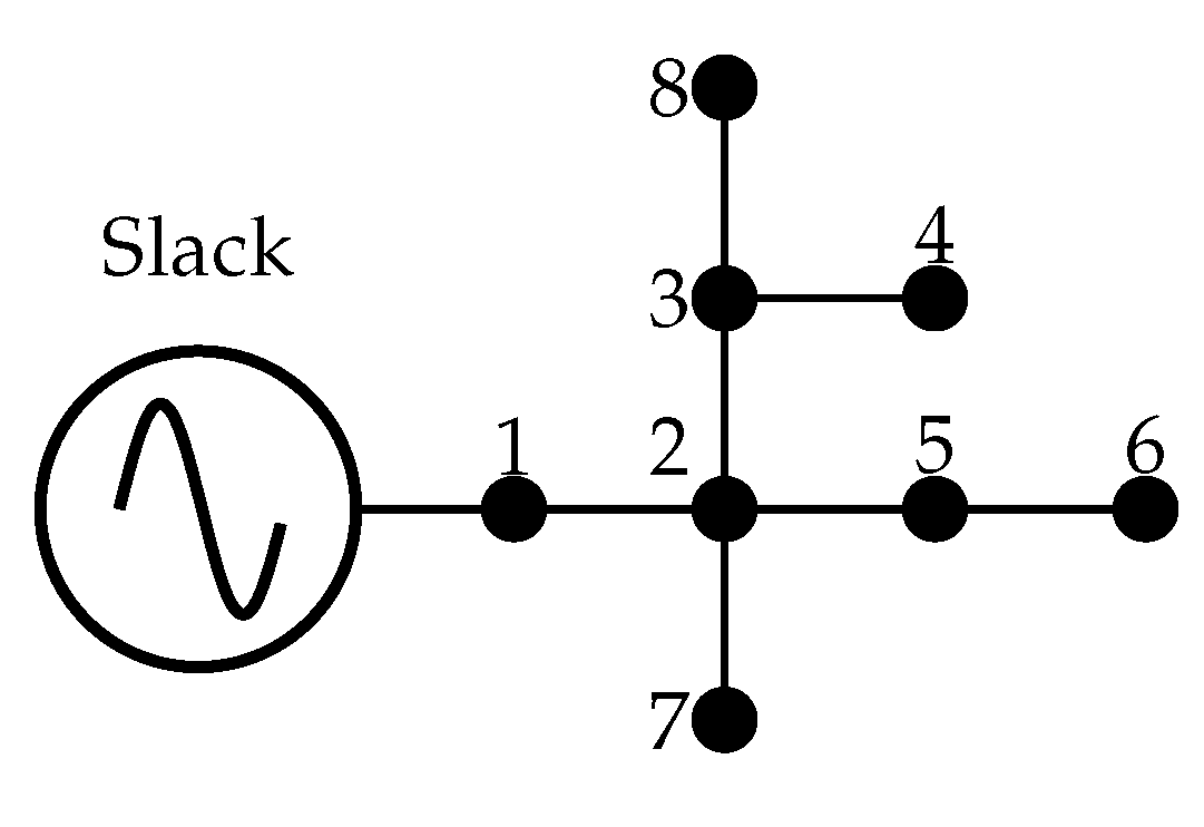
5.1. Results for the 8-Node System

Table 3. Performance of the power losses after implementing the phase-swapping plan in the 8-bus test feeder.

Method	Connections	Losses (kW)	Std. (kW)	Reduction (%)	Proc. Time (s)
Benchmark case	$\left\{1,1,1,1,1,1,1\right\}$	13.9925	-	-	-
CBGA [15]	$\left\{6,1,5,1,4,4,1\right\}$	10.5869	0.0897	24.34	2.8137
VSA [15]	$\left\{6,1,5,1,2,1,1\right\}$	10.5869	$4\times {10}^{-4}$	24.34	6.059
CSA	$\left\{5,3,4,5,6,6,3\right\}$	10.5869	$4.646\times {10}^{-3}$	24.34	8.7290
ICSA	$\left\{2,4,5,4,6,4,3\right\}$	10.5869	$1.099\times {10}^{-5}$	24.34	47.7428

shows the results obtained by the proposed ICSA for the 8-node test system as follows: (i) all methodologies allow a reduction of more than 24% in total power losses; (ii) the solution obtained with the ICSA for the 8-node system equals those reported in [15], which states that the optimal global solution for this system is 10.5968 kW, albeit with a much longer processing time; and (iii) the standard deviation for the ICSA shown in Table 3 is $1.099\times {10}^{-5}$ kW, which is at least ten times lower than in the VSA [15]. These results indicate that the repeatability of the solutions is close to 100% when solving the phase swapping problem in the 8-node test system, bearing in mind that the solution space has dimensions of 279,936.

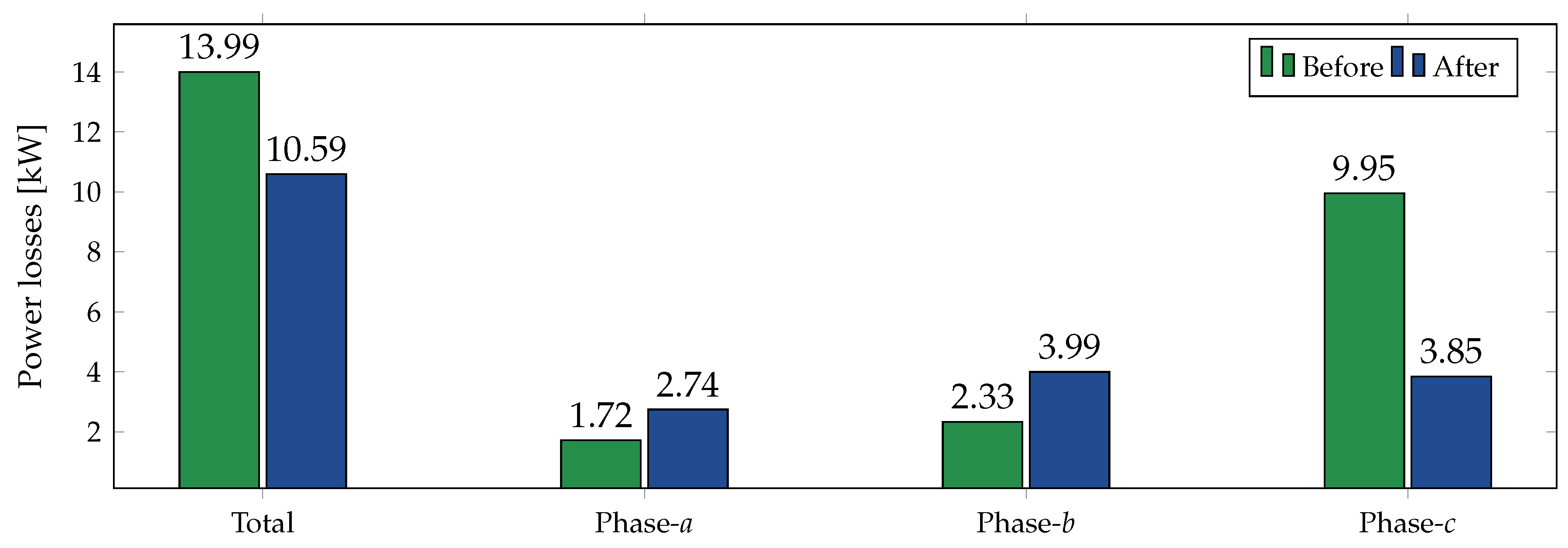
Figure 4 displays the variations of the phase power losses before and after the application of phase swapping with the ICSA, where the phase losses of a and b increase by 1.025 kW and 1.663 kW, respectively. On the contrary, the power losses in the electrical phase c decrease by about 6.10 kW, which increases the offsets seen in the power losses of phases a and b. Additionally, the power losses per phase are close to the average of the total power losses of approximately 3.50 kW, with differences of less than 0.80 kW. These results indicate that phase swapping by ICSA is an effective way to redistribute the loads in the phases of the system as evenly as possible.

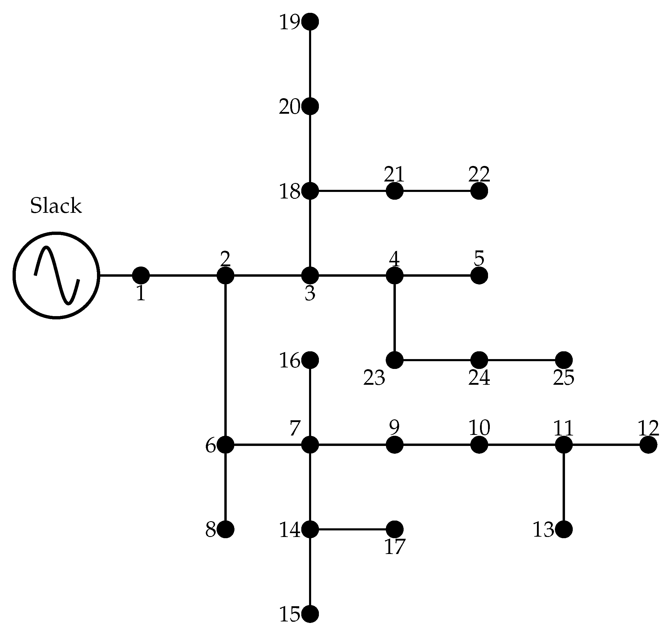
5.2. Results for the 25-Node System

Table 4. Performance of the power losses after implementing the phase-swapping plan in the 25-bus test feeder.

Method	Connections	Losses (kW)	Std. (kW)	Proc. Time (s)
Benchmark case	$\left\{1,1,1,1,1,1,1,1,1,1,1,1,1,1,1,1,1,1,1,1,1,1,1,1\right\}$	75.4207	-	-
CBGA [15]	$\left\{1,1,3,5,2,1,1,1,2,6,5,1,5,3,6,6,3,3,1,3,5,2,4,3\right\}$	72.2919	0.0366	18.6683
VSA [15]	$\left\{1,2,4,5,6,1,2,3,1,5,4,3,3,5,5,2,3,3,5,4,2,2,2,3\right\}$	72.2888	0.0233	36.6900
CSA	$\left\{4,4,4,2,6,5,2,5,3,6,3,1,4,2,2,1,2,3,3,5,2,5,3,4\right\}$	72.3296	0.0225	29.4161
ICSA	$\left\{4,2,4,5,6,3,2,3,1,5,4,3,3,5,5,2,3,3,5,4,2,2,2,3\right\}$	72.2888	0.0116	134.8935

shows the results obtained by the proposed ICSA for the 25-node test system, where the following is evident: (i) the solution obtained with the ICSA for the 25-node system equals the one reported in [15] for the VSA, which states that the optimal global solution for this system is 72.2888 kW; (ii) the solution obtained with the ICSA for the 25-node system outperforms the solution obtained with the CSA, which shows that the improvement made to the classical CSA explores and exploits the solution space for systems of large dimensions (i.e., 24 nodes in this case) in a better way; and (iii) the standard deviation for the ICSA, shown in Table 4, is 0.0116 kW lower than those reported in [15] and in CSA. This affirms the repeatability properties of the ICSA for solving the phase swapping problem, considering the size of the solution space, i.e., $2.8430\times {10}^{19}$.

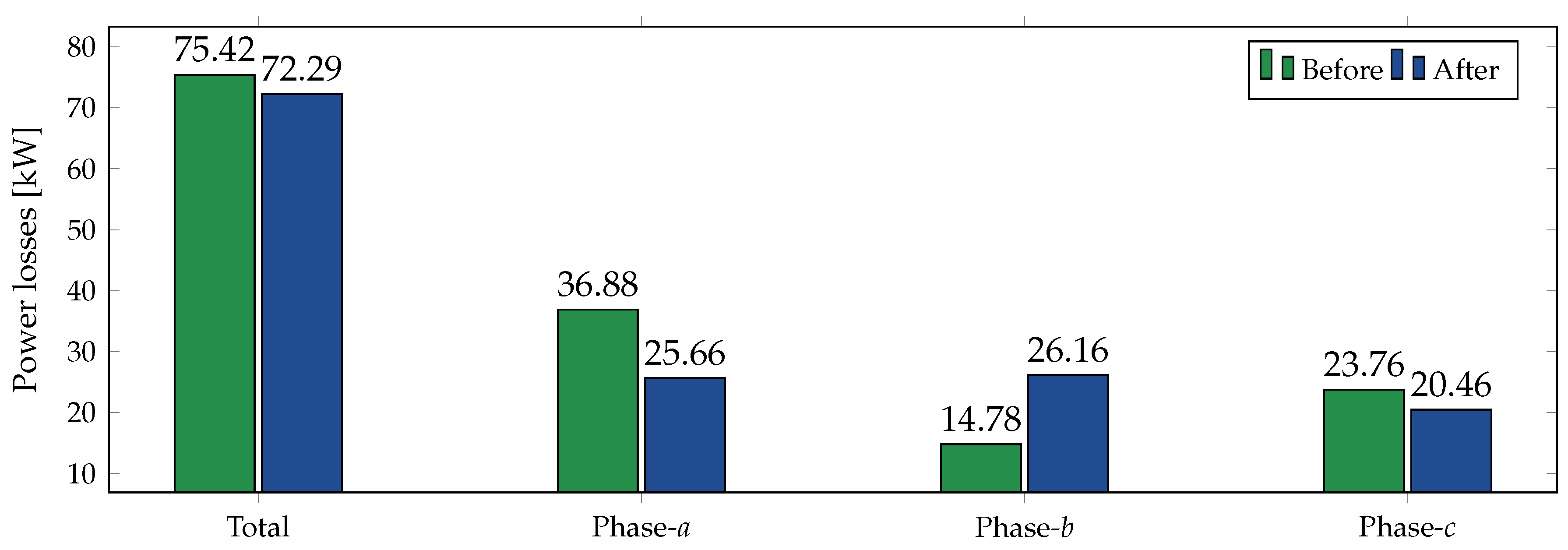
Figure 5 represents the variations of the phase power losses before and after the application of phase swapping with the ICSA, where the phase losses of b increase by 11.3776 kW. On the other hand, the phase power losses of a and c approximately decrease by 11.2156 kW and 3.294 kW, respectively, which offsets the increase seen in the electrical phase b power losses. Additionally, the phase power losses are close to the average of the total power losses, approximately 24 kW, with differences of less than 3.60 kW. These results indicate that phase swapping by ICSA is an effective way to redistribute the loads in the phases of the system as evenly as possible.

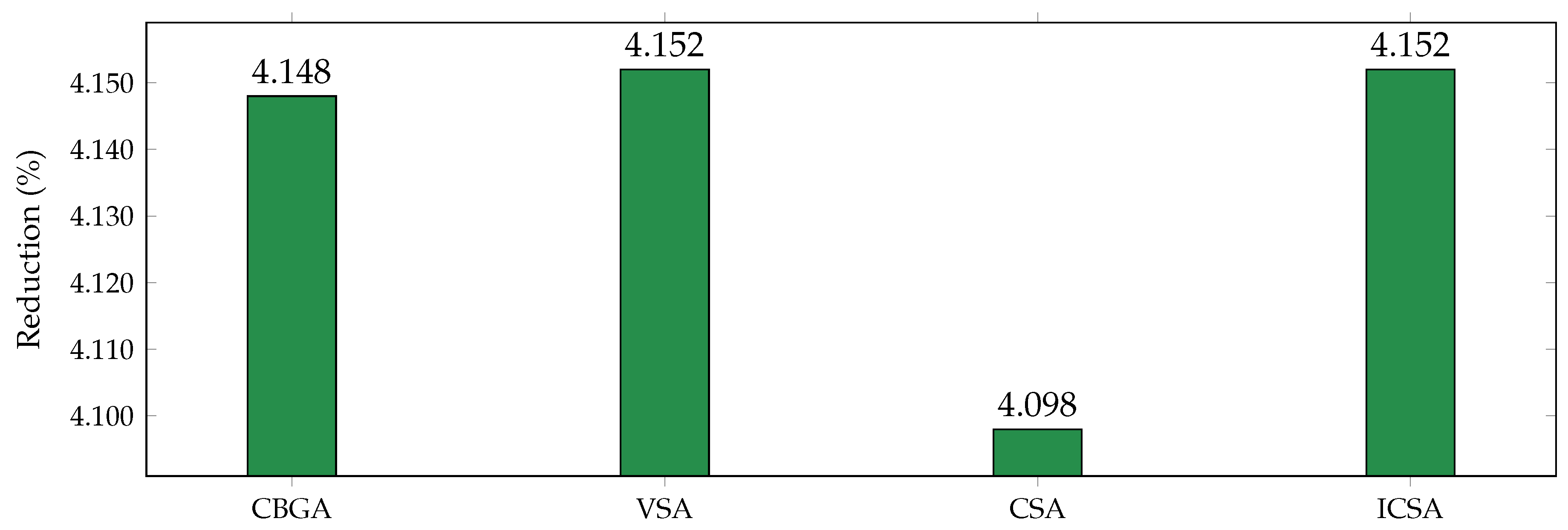
Figure 6 shows a comparison of the percentage reductions of the total active power losses of the different methods displayed in Table 4, in contrast to the initial power losses. All methodologies allow a cutback of more than 4%. ICSA obtains a reduction of 4.15%, akin to the VSA reported in [15].

5.3. Results for the 37-Node System

Table 5. Performance of the power losses after implementing the phase-swapping plan in the 37-bus test feeder.

Method	Connections	Losses (kW)	Std. (kW)	Proc. Time (s)
Benchmark case	{1,1,1,1,1,1,1,1,1,1,1,1,1,1,1,1,1,1,1,1,1,1,1,1	76.1357	-	-
	1,1,1,1,1,1,1,1,1,1,1}
CBGA [15]	{4,1,1,6,4,4,6,4,1,1,6,5,2,1,2,3,1,5,1,4,3,2,6,5	61.5785	0.4274	14.1816
	3,2,1,6,5,2,1,4,1,2,3}
VSA [15]	{4,1,1,5,3,4,2,3,1,1,3,2,2,1,3,5,2,3,1,3,6,1,2,3	61.4801	0.3286	50.0262
	3,2,1,1,2,4,1,4,1,2,4}
CSA	{4,5,4,4,4,4,5,4,3,3,4,4,1,4,5,3,3,2,3,3,4,3,4,3	61.6565	0.2975	89.1698
	3,4,4,4,5,4,4,4,3,2,3}
ICSA	{4,4,4,3,5,3,3,5,6,5,3,2,4,5,3,5,5,3,5,5,6,5,2,6	61.4781	0.1344	238.3614
	6,4,6,5,4,4,3,2,5,4,2}

shows the results obtained by the proposed ICSA for the 37-node test system, where the following is evident: (i) the solution obtained with the ICSA for the 37-node system improves the one reported in [15] for the VSA, which indicates that the optimal solution for this system is 61.4781 kW; (ii) the solution obtained with the ICSA for the 37-node system outperforms the solution obtained with the CSA, which shows that the improvement made to the classical CSA explores and exploits the solution space for systems of large dimensions (i.e., 37-nodes) in a better way; and (iii) the standard deviation for the ICSA shown in Table 5 is 0.1344 kW, which is lower than those reported in [15] and the one obtained by the CSA. This affirms the repeatability properties of the ICSA for solving the phase swapping problem, considering the size of the solution space, i.e., $6.1887\times {10}^{28}$.

Figure 7 portrays the variations of the phase power losses before and after the application of phase swapping with the ICSA, where the phase b losses increase by 9.9184 kW. On the contrary, the phase power losses in a and c decrease by approximately 6.7771 kW and 17.7989 kW, respectively, offsetting the increase seen in the electrical phase b power losses. Additionally, the phase power losses are close to the average total power losses of approximately 20.50 kW, with differences of less than 1.40 kW. These results indicate that phase swapping by ICSA is an effective way to redistribute the loads in the phases of the system as evenly as possible.

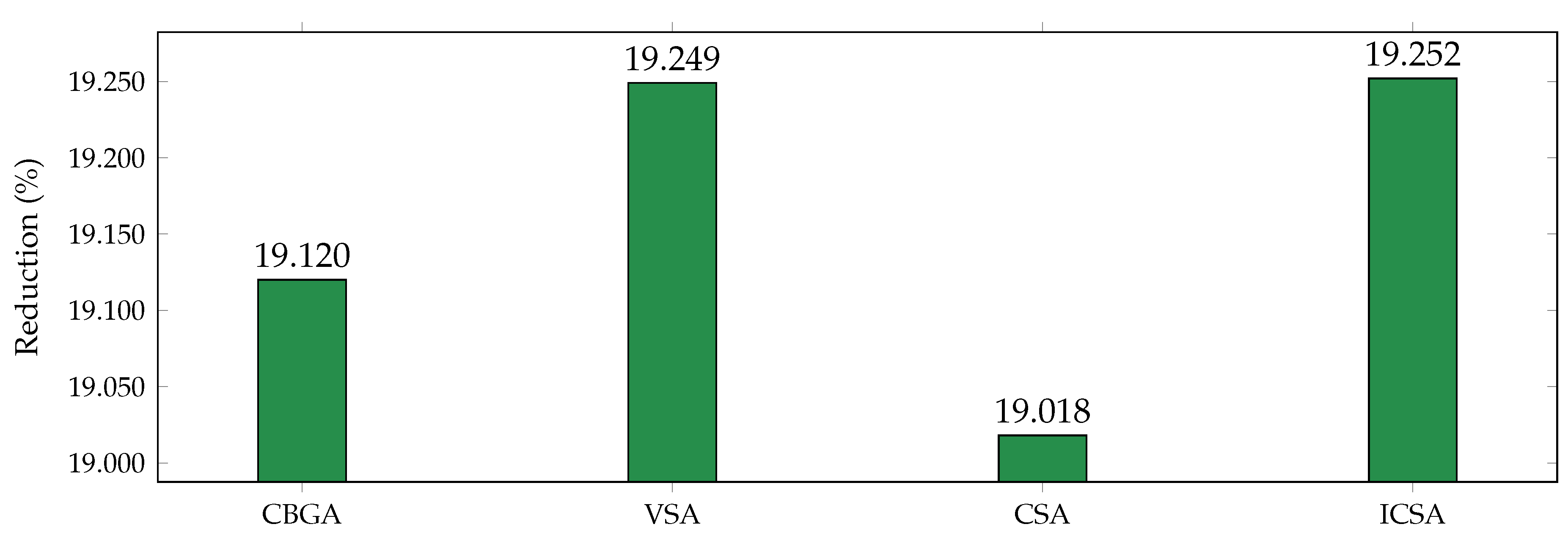
Figure 8 compares the reductions in the total active power losses percentage of the different methods presented in Table 5 to the initial power losses. All methodologies allow a decrease of more than 19%, where ICSA obtains a reduction of 19.252%, a higher loss than VSA, as reported in [15], which reported a decrease of 19.249%.

In Figure 8, it is possible to observe that the proposed ICSA allows an additional improvement about 0.003% when compared to the power losses reduction with the VSA. This reduction implies a difference of 0.1784 kW in the total power losses minimization for the IEEE 37-bus system. Even if this power losses value corresponds to a small power losses reduction for this system, this demonstrates that the proposed ICSA finds an optimal solution for the IEEE 37-bus system, which supports the best current literature report obtained by [15] with the VSA method. Thus, this new solution will serve as a reference point for future approaches that can be proposed to solve the phase swapping problem in ADSs.

5.4. Complementary Results

The following can be concluded from the results obtained in Section 5.

✓

The optimal solution achieved with the enhanced version of the CSA for each test system is equal to the one reported in [15] for the 8- and 25-node systems. However, it obtained a better solution for the 37-node system. Note that the obtained solutions (power losses) in this research are 10.5869 kW, 72.2888 kW, and 61.4781 kW for the 8-, 25-, and 37-node systems, respectively, while the best solutions reported in [15] are 10.5869 kW, 72.2888 kW, and 61.4801 kW, respectively. It is relevant to highlight that the ICSA requires a longer processing time. Nevertheless, these times do not exceed 6 minutes, which is not significant considering the terms for optimization problems with solution spaces with hundreds of thousands of combinations. It ensures excellent quality solutions and even better ones than the values reported in the literature review in some cases (see results for the 37-node system). However, simulations in tests feeders with large number of nodes will be required to ensure that, in all of the cases, the processing times spent by the proposed ICSA will be compensated with optimal solutions better than the solutions provided by the VSA.

✓

The standard deviations reported in Table 3, Table 4 and Table 5 for the 8-, 25-, and 37-node systems, respectively, for ICSA are lower than those reported in [15]. In addition, a standard deviation of 0.1344 kW for the 37-node test system demonstrates the repeatability properties of the ICSA for solving the phasing problem, considering that the dimensions of the solution space are higher than $1\times {10}^{28}$. Regarding metaheuristic optimization methods, the main preoccupation in the literature is associated with the ability of these methods to find the same optimal solution at each simulation. However, this is not possible due to the random nature of the exploration and exploitation criteria inside of each metaheuristic optimizer. Nevertheless, when an optimization methodology exhibits low standard deviations, all the solutions are contained inside of a small hyper-sphere close to the global optimum. This improves the optimization method of the proposed ICSA when compared with a family of metaheuristic optimizers.

✓

When comparing the base cases of each test system with the proposed methodologies, as shown in Table 3 and Figure 5 and Figure 7, the reductions in energy losses resulting from ICSA in the 8, 25, and 37-node systems are 24.34%, 4.152%, and 19.252%, respectively. The results show that better results are obtained when applying the proposed methodology for the 37-node system, in contrast to the CSA and the VSA [15]. Likewise, it is observed that the proposed enhancement for the CSA effectively explores and exploits the solution space for large systems higher than 25 nodes in the case of distribution power systems.

✓

The comparison of the effect in the energy losses redistribution at each phase using the classic and improved CSA methods is presented in

Table 6. Comparison between the CSA and the proposed ICSA regarding power losses among phases.

Method	Phase a (kW)	Phase b (kW)	Phase b (kW)	Total (kW)
8-bus system
Benchmark case	1.7158	2.3305	9.9462	13.9925
CSA	3.7617	2.7295	4.0957	10.5869
ICSA	2.7412	3.9930	3.8464	10.5869
25-bus system
Benchmark case	36.8801	14.7837	23.7570	75.4207
CSA	24.9590	26.2079	21.1627	72.3296
ICSA	25.6645	26.1613	20.4630	72.2888
IEEE 37-bus system
Benchmark case	27.1532	11.9143	37.0683	76.1357
CSA	19.1177	20.5926	21.1627	61.6565
ICSA	20.3761	21.8327	19.2694	61.4781

.

With these results, we can make several observations. (i) In the 8-bus system, the phase c presents power losses higher than 4 kW, while the ICSA does not support this value; however, both solutions are indeed optimal since the total power losses is the same for both methods. (ii) In the 25-bus system both methods, i.e., the CSA and its improved version, the phase c has been identified to present higher power losses surpassing 26 kW; however, regarding the final power losses, the ICSA presents better load redistribution, since the amount of power losses is about 0.0408 kW. Finally, (iii) in the 37-bus system, the CSA method presents a difference between phases a and b power losses of $2.0450$ kW, while the proposed ICSA has a minor difference between both phases with a value of $1.1067$ kW. This directly impacts the final grid results with a general improvement of about $0.1784$ kW in favor of the proposed ICSA, which is indeed the best global optimum reported in the current literature for the IEEE 37-bus system.

6. Conclusions and Future Works

This paper presented a master–slave methodology to solve the phase equilibrium problem in ADSs. For this purpose, an ICSA was proposed using the VSA evolution mechanism. The master stage determined the set of phase configurations for the system three-phase charges through the ICSA, using an integer encoding between 1 and 6 representing the load connections in the three-phase system. On the other hand, the slave stage evaluated each of the load connections in the TPPF, which correspond to the extended version of the iterative sweep power flow method for unbalanced three-phase systems.

The numerical results on the 8-, 25-, and 37-node test systems showed that the proposed ICSA, compared to the VSA, achieves identical solutions for the 8-node and 25-node systems. However, for the 37-node system, the ISCA obtains a better optimal solution when compared with the current report employing the VSA method. The solutions obtained by the ICSA are 10.5869 kW, 72.2888 kW, and 61.4781 kW for the 8-, 25-, and 37-node systems, representing a reduction of 24.34%, 4.152%, and 19.252%, respectively. In the same way, the solutions for the VSA are 10.5869 kW, 72.2888 kW, and 61.4801 kW, respectively.

In addition, the proposed methodology has minor standard deviations for solving the phase swapping problem for the 8-, 25-, and IEEE 37-node test systems, which were $1.099\times {10}^{-5}$ kW, 0.0116 kW, and 0.1344 kW, respectively. This demonstrates better repeatability properties of the improved algorithm, since all the solutions are contained inside small hyper-spheres around the global optimum. Further, the solution space for the phase equilibrium problem potentially increases as a function of the demand nodes. Thus, for the IEEE 37-node system, there is a solution space bigger than $1\times {10}^{28}$, which is by far higher than 100 billion combinations. This result confirmed the effectiveness of the proposed methodology for solving complex MINLP models such as the phase equilibrium problem in ADSs as well as in being better than the optimal solution reported in the current literature using the VSA.

In future work, it is possible to accomplish the following: (i) combine the proposed phase swapping with the optimal placement of distributed generators to reduce power losses in ADSs; (ii) employ typical active and reactive power demand curves to solve the phase swapping problem using the ICSA to reduce power losses; and (iii) use the ICSA to solve the optimal reconfiguration problem in three-phase radial distribution networks.

References

1. Montoya, O.D.; Serra, F.M.; De Angelo, C.H. On the efficiency in electrical networks with ac and dc operation technologies: A comparative study at the distribution stage. Electronics 2020, 9, 1352. [Google Scholar] [CrossRef]
2. Montoya, O.D.; Gil-González, W.; Hernández, J.C. Efficient Operative Cost Reduction in Distribution Grids Considering the Optimal Placement and Sizing of D-STATCOMs Using a Discrete-Continuous VSA. Appl. Sci. 2021, 11, 2175. [Google Scholar] [CrossRef]
3. Nassar, M.E.; Salama, M. A novel branch-based power flow algorithm for islanded AC microgrids. Electr. Power Syst. Res. 2017, 146, 51–62. [Google Scholar] [CrossRef]
4. Aboshady, F.; Thomas, D.W.; Sumner, M. A wideband single end fault location scheme for active untransposed distribution systems. IEEE Trans. Smart Grid 2019, 11, 2115–2124. [Google Scholar] [CrossRef]
5. Montoya, O.D.; Arias-Londoño, A.; Grisales-Noreña, L.F.; Barrios, J.Á.; Chamorro, H.R. Optimal Demand Reconfiguration in Three-Phase Distribution Grids Using an MI-Convex Model. Symmetry 2021, 13, 1124. [Google Scholar] [CrossRef]
6. Arias, J.; Calle, M.; Turizo, D.; Guerrero, J.; Candelo-Becerra, J.E. Historical load balance in distribution systems using the branch and bound algorithm. Energies 2019, 12, 1219. [Google Scholar] [CrossRef] [Green Version]
7. Alvarado-Barrios, L.; Álvarez-Arroyo, C.; Escaño, J.M.; Gonzalez-Longatt, F.M.; Martinez-Ramos, J.L. Two-Level Optimisation and Control Strategy for Unbalanced Active Distribution Systems Management. IEEE Access 2020, 8, 197992–198009. [Google Scholar] [CrossRef]
8. Granada Echeverri, M.; Gallego Rendón, R.A.; López Lezama, J.M. Optimal phase balancing planning for loss reduction in distribution systems using a specialized genetic algorithm. Ing. Cienc. 2012, 8, 121–140. [Google Scholar] [CrossRef] [Green Version]
9. Hooshmand, R.; Soltani, S. Simultaneous optimization of phase balancing and reconfiguration in distribution networks using BF–NM algorithm. Int. J. Electr. Power Energy Syst. 2012, 41, 76–86. [Google Scholar] [CrossRef]
10. Ogunsina, A.A.; Petinrin, M.O.; Petinrin, O.O.; Offornedo, E.N.; Petinrin, J.O.; Asaolu, G.O. Optimal distributed generation location and sizing for loss minimization and voltage profile optimization using ant colony algorithm. SN Appl. Sci. 2021, 3, 1–10. [Google Scholar] [CrossRef]
11. Asadi, M.; Shokouhandeh, H.; Rahmani, F.; Hamzehnia, S.M.; Harikandeh, M.N.; Lamouki, H.G.; Asghari, F. Optimal placement and sizing of capacitor banks in harmonic polluted distribution network. In Proceedings of the 2021 IEEE Texas Power and Energy Conference (TPEC), College Station, TX, USA, 2–5 February 2021; pp. 1–6. [Google Scholar]
12. Jakus, D.; Čađenović, R.; Vasilj, J.; Sarajčev, P. Optimal reconfiguration of distribution networks using hybrid heuristic-genetic algorithm. Energies 2020, 13, 1544. [Google Scholar] [CrossRef] [Green Version]
13. Montoya, O.D.; Garces, A.; Castro, C.A. Optimal conductor size selection in radial distribution networks using a mixed-integer non-linear programming formulation. IEEE Lat. Am. Trans. 2018, 16, 2213–2220. [Google Scholar] [CrossRef]
14. Łukaszewski, A.; Nogal, Ł.; Robak, S. Weight Calculation Alternative Methods in Prime’s Algorithm Dedicated for Power System Restoration Strategies. Energies 2020, 13, 6063. [Google Scholar] [CrossRef]
15. Cortés-Caicedo, B.; Avellaneda-Gómez, L.S.; Montoya, O.D.; Alvarado-Barrios, L.; Chamorro, H.R. Application of the Vortex Search Algorithm to the Phase-Balancing Problem in Distribution Systems. Energies 2021, 14, 1282. [Google Scholar] [CrossRef]
16. Montoya, O.D.; Molina-Cabrera, A.; Grisales-Noreña, L.F.; Hincapié, R.A.; Granada, M. Improved Genetic Algorithm for Phase-Balancing in Three-Phase Distribution Networks: A Master-Slave Optimization Approach. Computation 2021, 9, 67. [Google Scholar] [CrossRef]
17. Saad Al-Sumaiti, A.; Kavousi-Fard, A.; Salama, M.; Pourbehzadi, M.; Reddy, S.; Rasheed, M.B. Economic Assessment of Distributed Generation Technologies: A Feasibility Study and Comparison with the Literature. Energies 2020, 13, 2764. [Google Scholar] [CrossRef]
18. Rajaram, R.; Kumar, K.S.; Rajasekar, N. Power system reconfiguration in a radial distribution network for reducing losses and to improve voltage profile using modified plant growth simulation algorithm with Distributed Generation (DG). Energy Rep. 2015, 1, 116–122. [Google Scholar] [CrossRef] [Green Version]
19. Ahshan, R. Analysis of Loss Reduction Techniques for Low Voltage Distribution Network. J. Eng. Res. [TJER] 2020, 17, 100–111. [Google Scholar]
20. Grigoraș, G.; Neagu, B.C.; Gavrilaș, M.; Triștiu, I.; Bulac, C. Optimal phase load balancing in low voltage distribution networks using a smart meter data-based algorithm. Mathematics 2020, 8, 549. [Google Scholar] [CrossRef] [Green Version]
21. Montoya, O.D.; Giraldo, J.S.; Grisales-Noreña, L.F.; Chamorro, H.R.; Alvarado-Barrios, L. Accurate and Efficient Derivative-Free Three-Phase Power Flow Method for Unbalanced Distribution Networks. Computation 2021, 9, 61. [Google Scholar] [CrossRef]
22. Taghipour Boroujeni, S.; Mardaneh, M.; Hashemi, Z. A dynamic and heuristic phase balancing method for LV feeders. Appl. Comput. Intell. Soft Comput. 2016, 2016. [Google Scholar] [CrossRef]
23. Gandomkar, M. Phase balancing using genetic algorithm. In Proceedings of the 39th International Universities Power Engineering Conference, 2004, UPEC 2004, Bristol, UK, 6–8 September 2004; Volume 1, pp. 377–379. [Google Scholar]
24. Rios, M.A.; Castaño, J.C.; Garcés, A.; Molina-Cabrera, A. Phase Balancing in Power Distribution Systems: A heuristic approach based on group-theory. In Proceedings of the 2019 IEEE Milan PowerTech, Milan, Italy, 23–27 June 2019; pp. 1–6. [Google Scholar]
25. Garces, A.; Gil-González, W.; Montoya, O.D.; Chamorro, H.R.; Alvarado-Barrios, L. A Mixed-Integer Quadratic Formulation of the Phase-Balancing Problem in Residential Microgrids. Appl. Sci. 2021, 11, 1972. [Google Scholar] [CrossRef]
26. Amon, D.A.; Adeyemi, A. A modified bat algorithm for power loss reduction in electrical distribution system. Indones. J. Electr. Eng. Comput. Sci. (IJEECS) 2015, 14, 55–61. [Google Scholar]
27. Sathiskumar, M.; Kumar, A.N.; Lakshminarasimman, L.; Thiruvenkadam, S. A self adaptive hybrid differential evolution algorithm for phase balancing of unbalanced distribution system. Int. J. Electr. Power Energy Syst. 2012, 42, 91–97. [Google Scholar] [CrossRef]
28. Zhu, J.; Bilbro, G.; Chow, M.Y. Phase balancing using simulated annealing. IEEE Trans. Power Syst. 1999, 14, 1508–1513. [Google Scholar] [CrossRef] [Green Version]
29. Askarzadeh, A. A novel metaheuristic method for solving constrained engineering optimization problems: Crow search algorithm. Comput. Struct. 2016, 169, 1–12. [Google Scholar] [CrossRef]
30. Dogan, B. A Modified Vortex Search Algorithm for Numerical Function Optimization. Int. J. Artif. Intell. Appl. 2016, 7, 37–54. [Google Scholar] [CrossRef]
31. Shen, T.; Li, Y.; Xiang, J. A graph-based power flow method for balanced distribution systems. Energies 2018, 11, 511. [Google Scholar] [CrossRef] [Green Version]
32. Herrera-Briñez, M.C.; Montoya, O.D.; Alvarado-Barrios, L.; Chamorro, H.R. The Equivalence between Successive Approximations and Matricial Load Flow Formulations. Appl. Sci. 2021, 11, 2905. [Google Scholar] [CrossRef]
33. Łukaszewski, A.; Nogal, Ł. Influence of lightning current surge shape and peak value on grounding parameters. Bull. Pol. Acad. Sci. Tech. Sci. 2021, 69, e136730. [Google Scholar] [CrossRef]
34. Gil-González, W.; Montoya, O.D.; Rajagopalan, A.; Grisales-Noreña, L.F.; Hernández, J.C. Optimal Selection and Location of Fixed-Step Capacitor Banks in Distribution Networks Using a Discrete Version of the Vortex Search Algorithm. Energies 2020, 13, 4914. [Google Scholar] [CrossRef]
35. Doğan, B.; Ölmez, T. A new metaheuristic for numerical function optimization: Vortex Search algorithm. Inf. Sci. 2015, 293, 125–145. [Google Scholar] [CrossRef]
36. Hussien, A.G.; Amin, M.; Wang, M.; Liang, G.; Alsanad, A.; Gumaei, A.; Chen, H. Crow Search Algorithm: Theory, Recent Advances, and Applications. IEEE Access 2020, 8, 173548–173565. [Google Scholar] [CrossRef]
37. Jain, M.; Rani, A.; Singh, V. An improved Crow Search Algorithm for high-dimensional problems. J. Intell. Fuzzy Syst. 2017, 33, 3597–3614. [Google Scholar] [CrossRef]
38. Clayton, N.; Emery, N. Corvid cognition. Curr. Biol. 2005, 15, R80–R81. [Google Scholar] [CrossRef] [Green Version]
39. Askarzadeh, A. Capacitor placement in distribution systems for power loss reduction and voltage improvement: A new methodology. IET Gener. Transm. Distrib. 2016, 10, 3631–3638. [Google Scholar] [CrossRef]
40. Rajput, S.; Parashar, M.; Dubey, H.M.; Pandit, M. Optimization of benchmark functions and practical problems using Crow Search Algorithm. In Proceedings of the 2016 Fifth International Conference on Eco-friendly Computing and Communication Systems (ICECCS), Bhopal, India, 8–9 December 2016; pp. 73–78. [Google Scholar]
41. Díaz, P.; Pérez-Cisneros, M.; Cuevas, E.; Avalos, O.; Gálvez, J.; Hinojosa, S.; Zaldivar, D. An improved crow search algorithm applied to energy problems. Energies 2018, 11, 571. [Google Scholar] [CrossRef] [Green Version]
42. Li, Z.; Wang, W.; Yan, Y.; Li, Z. PS–ABC: A hybrid algorithm based on particle swarm and artificial bee colony for high-dimensional optimization problems. Expert Syst. Appl. 2015, 42, 8881–8895. [Google Scholar] [CrossRef]
43. Sayed, G.I.; Hassanien, A.E.; Azar, A.T. Feature selection via a novel chaotic crow search algorithm. Neural Comput. Appl. 2019, 31, 171–188. [Google Scholar] [CrossRef]
44. Li, P.; Zhao, Y. A quantum-inspired vortex search algorithm with application to function optimization. Nat. Comput. 2019, 18, 647–674. [Google Scholar] [CrossRef]
45. Montoya, O.D.; Grisales-Noreña, L.F.; Amin, W.T.; Rojas, L.A.; Campillo, J. Vortex Search Algorithm for Optimal Sizing of Distributed Generators in AC Distribution Networks with Radial Topology. In Workshop on Engineering Applications; Springer: Berlin/Heidelberg, Germany, 2019; pp. 235–249. [Google Scholar] [CrossRef]
Figure 1. Electrical design of the 8-node system.
Symmetry 13 01329 g001
Figure 2. Electrical design of the 25-node system.
Symmetry 13 01329 g002
Figure 3. Electrical design of the 37-node system.
Symmetry 13 01329 g003
Figure 4. Effect of phase swapping on power losses in the 8-bus test feeder.
Symmetry 13 01329 g004
Figure 5. Effect of phase swapping on power losses in the 25-bus test feeder.
Symmetry 13 01329 g005
Figure 6. Reduction of the power losses in the 25-bus system.
Symmetry 13 01329 g006
Figure 7. Effect of phase swapping on power losses in the 37-bus test feeder.
Symmetry 13 01329 g007
Figure 8. Reduction of the power losses in the 37-bus test feeder.
Symmetry 13 01329 g008