Fractional Dual-Phase Lag Equation—Fundamental Solution of the Cauchy Problem

Abstract

In the paper, a fundamental solution of the fractional dual-phase-lagging heat conduction problem is obtained. The considerations concern the 1D Cauchy problem in a whole-space domain. A solution of the initial-boundary problem is determined by using the Fourier–Laplace transform technique. The final form of solution is given in a form of a series. One of the properties of the derived fundamental solution of the considered problem with the initial condition expressed be the Dirac delta function is that it is symmetrical. The effect of the time-fractional order of the Caputo derivatives and the phase-lag parameters on the temperature distribution is investigated numerically by using the method which is based on the Fourier-series quadrature-type approximation to the Bromwich contour integral.

1. Introduction

In recent years, we have observed a significant increase in interest in fractional calculus, which is used not only in engineering but also in other sciences such as biology or economics. This is due to the fact that scientists are looking increasingly accurate descriptions of physical phenomena and processes. Methods for solving fractional differential equations as well as basic properties of fractional integrals and derivatives can be found in many books [1,2] and papers [3,4]. We use fractional calculus primarily for the mathematical modelling of physical phenomena such as, for example, heat conduction [5,6]. The starting point for considerations of many authors is the classical theory of heat transfer based on Fourier’s law. However, this model has a certain non-physical property, i.e., the speed of heat is infinite. To eliminate this unreal property, a phase-lag parameter into the classical Fourier’s law is introduced. Many researchers use a dual-phase-lag model along with a single phase-lag model [7,8]. This model can be used especially for the mathematical description of phenomena occurring in the microscale, e.g., in heating the thin film [7,9].

Widely used in analytical solving of many engineering problems with specified boundary conditions and/or initial conditions is Green’s function method [10,11]. The advantage of the Green’s function method is that we can use the Green function even to express the solution of non-homogeneous problems. Many examples of the application of this method to the problem of heat conduction can be found in books [12,13]. The advantage of this method is that the Green’s function always exists, but in the case of a more complex domain, it cannot always be written explicitly. In this case, we can use the method of separation of variables or the Fourier–Laplace transform method [14,15]. In reference [16], the fundamental solutions to the Cauchy and Dirichlet 1D problems based upon a heat conduction equation contained the Caputo–Fabrizio derivative is considered.

In this paper, we presented a fundamental solution of the fractional dual-phase-lag equation of heat transfer with appropriate initial-boundary conditions. Here, the considerations are limited and applied only to one-dimensional Cauchy problem with initial functions defined on whole-space domain. A solution of the problem is determined by using the Fourier–Laplace transform technique. The final solution of the equation is obtained in the form of an infinite sum of functions. The effect of the time-fractional derivative orders and the phase-lag parameters on the temperature distribution in the space was investigated. In the final part of the paper, several examples concerning the analysis of temperature distribution are presented.

2. Formulation of the Problem

The classical Fourier’s law of the heat conduction describes the relation between the heat flux vector and gradient of temperature. The most commonly used model is in which the heat flow is described by the following parabolic equation:

$$q\left(x,t\right)=-\mathsf{\lambda } \nabla T\left(x,t\right)$$

(1)

where $x$ represents the spatial coordinates, $t$ is the time, $q$ is the heat flux vector, $\mathsf{\lambda }$ is the thermal conductivity, and $\nabla T$ is the temperature gradient. In this model, it is assumed, however, that the speed of heat propagation is infinite. Therefore, in recent years, non-Fourier constitutive models have been introduced, such as the Cattaneo model or the phase-lagging model [9]. For example, the Dual-Phase Lag (DPL) model is expressed by the equation:

$$q\left(x,t+{\mathsf{\tau }}_q\right)=-\mathsf{\lambda } \nabla T\left(x,t+{\mathsf{\tau }}_T\right)$$

(2)

where ${\mathsf{\tau }}_q$ and ${\mathsf{\tau }}_T$ are the thermodynamic properties of material called the thermal relaxation and thermalization times, respectively. Equation (2) describes a situation where the heat flux and temperature gradient occur during the heat transfer at different times. It is worth mentioning that for ${\mathsf{\tau }}_T=0$, Equation (2) represents the Cattaneo heat transfer model and for ${\mathsf{\tau }}_q={\mathsf{\tau }}_T=0$, Equation (2) reduces to the classical Fourier law.

In many works (i.e., [7]), both sides of Equation (2) are expanded using the classical Taylor series. In the discussed problem, we use the generalized/fractional expansion of function in the Taylor series [17] of the fractional order $\mathsf{\alpha }\in (0,1]$, which for the function $f$ near $\mathsf{\tau }$ is expressed by the following form:

$$\begin{array}{l}f\left(·,t+\mathsf{\tau }\right)={\displaystyle \sum _{k=0}^{\infty }\frac{{\mathsf{\tau }}^{k\mathsf{\alpha }}}{\Gamma \left(\mathsf{\alpha }k+1\right)} \frac{{}^C\partial ^{k\mathsf{\alpha }}f\left(·,t\right)}{\partial t^{k\mathsf{\alpha }}}}\\ \hspace{1em}\hspace{1em}\hspace{1em}\hspace{1em}=f\left(·,t\right)+\frac{{\mathsf{\tau }}^{\mathsf{\alpha }}}{\Gamma \left(\mathsf{\alpha }+1\right)}\frac{{}^C\partial ^{k\mathsf{\alpha }}f\left(·,t\right)}{\partial t^{\mathsf{\alpha }}}+\frac{{\mathsf{\tau }}^{2\mathsf{\alpha }}}{\Gamma \left(2\mathsf{\alpha }+1\right)}\frac{{}^C\partial {}^{2\mathsf{\alpha }}f\left(·,t\right)}{\partial t^{2\mathsf{\alpha }}}+\dots \end{array}$$

(3)

where:

$$\frac{{}^C\partial ^{\mathsf{\alpha }}f\left(·,t\right)}{\partial t^{\mathsf{\alpha }}}:=\left\{\begin{array}{ll}\frac{1}{\Gamma \left(1-\mathsf{\alpha }\right)}{\displaystyle \underset{0}{\overset{t}{\int }}\frac{1}{{\left(t-u\right)}^{\mathsf{\alpha }}}\frac{\partial f\left(·,u\right)}{\partial u}\mathrm{d}u}\hfill & \mathrm{for} \mathsf{\alpha }\in \left(0,1\right)\hfill \\ \frac{\partial f\left(·,t\right)}{\partial t}\hfill & \mathrm{for} \mathsf{\alpha }=1\hfill \end{array}\right.$$

(4)

is the fractional derivative of function $f\left(·,t\right)$ of order $\mathsf{\alpha }\in (0,1]$ defined in the Caputo sense [1,2] while:

$$\frac{{}^C\partial ^{k\mathsf{\alpha }}f\left(·,t\right)}{\partial t^{k_{\mathsf{\alpha }}}}:=\underset{k \mathrm{times}}{\underbrace{\frac{{}^C\partial ^{\mathsf{\alpha }}}{\partial t^{\mathsf{\alpha }}}\frac{{}^C\partial ^{\mathsf{\alpha }}}{\partial t^{\mathsf{\alpha }}}\frac{{}^C\partial ^{\mathsf{\alpha }}}{\partial t^{\mathsf{\alpha }}}\cdots \frac{{}^C\partial ^{\mathsf{\alpha }}}{\partial t^{\mathsf{\alpha }}}}}f\left(·,t\right) \mathrm{for} k\in \mathbb{N}$$

(5)

and $\Gamma$ denotes the Gamma function.

In this work, only the first two terms of the generalized Taylor series are used. Thus, the first-order approximations for the heat flux $q\left(x,t+{\mathsf{\tau }}_q\right)$ and temperature $T\left(x,t+{\mathsf{\tau }}_T\right)$ (of orders ${\mathsf{\alpha }}_q\in (0,1]$ and ${\mathsf{\alpha }}_T\in (0,1]$, respectively) appearing in Equation (2) are as follows:

$$q\left(x,t+{\mathsf{\tau }}_q\right)=q\left(x,t\right)+\frac{{\mathsf{\tau }}_q^{{\mathsf{\alpha }}_q}}{\Gamma \left({\mathsf{\alpha }}_q+1\right)}\frac{{}^C{\partial }^{{\mathsf{\alpha }}_q}q\left(x,t\right)}{\partial t^{{\mathsf{\alpha }}_q}}$$

(6)

$$T\left(x,t+{\mathsf{\tau }}_T\right)=T\left(x,t\right)+\frac{{\mathsf{\tau }}_T^{{\mathsf{\alpha }}_T}}{\Gamma \left({\mathsf{\alpha }}_T+1\right)}\frac{{}^C{\partial }^{{\mathsf{\alpha }}_T}T\left(x,t\right)}{\partial t^{{\mathsf{\alpha }}_T}}$$

(7)

Introducing Formulas (6) and (7) into Equation (2), we obtained the heat conduction constitutive equation in the following form:

$$q\left(x,t\right)+\frac{{\mathsf{\tau }}_q^{{\mathsf{\alpha }}_q}}{\Gamma \left({\mathsf{\alpha }}_q+1\right)}\frac{{}^C{\partial }^{{\mathsf{\alpha }}_q}q\left(x,t\right)}{\partial t^{{\mathsf{\alpha }}_q}}=-\mathsf{\lambda } \left(\nabla T\left(x,t\right)+\frac{{\mathsf{\tau }}_T^{{\mathsf{\alpha }}_T}}{\Gamma \left({\mathsf{\alpha }}_T+1\right)}\frac{{}^C{\partial }^{{\mathsf{\alpha }}_T}\nabla T\left(x,t\right)}{\partial t^{{\mathsf{\alpha }}_T}}\right)$$

(8)

To derive the heat conduction equation, the energy conservation equation was used:

$$c\mathsf{\rho }\frac{\partial T\left(x,t\right)}{\partial t}=-\nabla ·q\left(x,t\right)+Q\left(x,t\right)$$

(9)

where $c$ is a specific heat of the medium, $\mathsf{\rho }$ is the density of the material, and the function $Q\left(x,t\right)$ is a capacity of internal heat sources.

We needed to combine Equation (8) with Equation (9) to eliminate the heat flux vector. For this, on both sides of the Equation (8) we apply the divergence operator and we got the following equation:

$$\nabla ·q\left(x,t\right)+\frac{{\mathsf{\tau }}_q^{{\mathsf{\alpha }}_q}}{\Gamma \left({\mathsf{\alpha }}_q+1\right)}\frac{{}^C{\partial }^{{\mathsf{\alpha }}_q}\nabla ·q\left(x,t\right)}{\partial t^{{\mathsf{\alpha }}_q}}=-\nabla ·\left[\mathsf{\lambda } \left(\nabla T\left(x,t\right)+\frac{{\mathsf{\tau }}_T^{{\mathsf{\alpha }}_T}}{\Gamma \left({\mathsf{\alpha }}_T+1\right)}\frac{{}^C{\partial }^{{\mathsf{\alpha }}_T}\nabla T\left(x,t\right)}{\partial t^{{\mathsf{\alpha }}_T}}\right)\right].$$

(10)

Then, from Equation (9) we determine the term of divergence and introduce it into Equation (8). Finally, we obtained the Fractional Dual-Phase Lag (FDPL) equation in the following form:

$$\begin{array}{cc}\hfill c\mathsf{\rho }\left(\frac{\partial T\left(x,t\right)}{\partial t}+\frac{{\mathsf{\tau }}_q^{{\mathsf{\alpha }}_q}}{\Gamma \left({\mathsf{\alpha }}_q+1\right)}\frac{{}^C{\partial }^{{\mathsf{\alpha }}_q+1}T\left(x,t\right)}{\partial t^{{\mathsf{\alpha }}_q+1}}\right)=& \nabla ·\left[\mathsf{\lambda } \left(\nabla T\left(x,t\right)+\frac{{\mathsf{\tau }}_T^{{\mathsf{\alpha }}_T}}{\Gamma \left({\mathsf{\alpha }}_T+1\right)}\frac{{}^C{\partial }^{{\mathsf{\alpha }}_T}\nabla T\left(x,t\right)}{\partial t^{{\mathsf{\alpha }}_T}}\right)\right]\hfill \\ & +Q\left(x,t\right)+\frac{{\mathsf{\tau }}_q^{{\mathsf{\alpha }}_q}}{\Gamma \left({\mathsf{\alpha }}_q+1\right)}\frac{{}^C{\partial }^{{\mathsf{\alpha }}_q}Q\left(x,t\right)}{\partial t^{{\mathsf{\alpha }}_q}}\hfill \end{array}.$$

(11)

Equation (11) is complemented by the following initial conditions:

$${\left.T\left(x,t\right)\right|}_{t=0}=T_0\left(x\right),$$

(12)

$${\left.\frac{\partial T\left(x,t\right)}{\partial t}\right|}_{t=0}=T_1\left(x\right)$$

(13)

and by the appropriate boundary conditions that depend on the problem under consideration and the computational domain.

It should be noted that for ${\mathsf{\alpha }}_T={\mathsf{\alpha }}_q=1$, Equation (11) becomes the classical first-order dual-phase lag heat transfer equation [7]:

$$c\mathsf{\rho }\left(\frac{\partial T\left(x,t\right)}{\partial t}+{\mathsf{\tau }}_q^{}\frac{{\partial }^{2}T\left(x,t\right)}{\partial t^2}\right)=\nabla ·\left[\mathsf{\lambda } \left(\nabla T\left(x,t\right)+{\mathsf{\tau }}_T^{}\frac{\partial \nabla T\left(x,t\right)}{\partial t}\right)\right]+Q\left(x,t\right)+{\mathsf{\tau }}_q^{}\frac{\partial Q\left(x,t\right)}{\partial t}$$

(14)

and for ${\mathsf{\tau }}_T={\mathsf{\tau }}_q=0$, Equation (11) reduces to the classical Fourier heat transfer equation:

$$c\mathsf{\rho }\frac{\partial T\left(x,t\right)}{\partial t}=\nabla ·\left[\mathsf{\lambda } \nabla T\left(x,t\right)\right]+Q\left(x,t\right).$$

(15)

3. Solution of 1D FDPL Equation

We searched for the solution of a 1D Cauchy problem in a whole-space domain, so $x=\left\{x\right\}$. Moreover, we assumed that $\mathsf{\lambda }$ is constant and $Q\left(x,t\right)=0$. For such a problem, the governing equation is written as:

$$c\mathsf{\rho }\left(\frac{\partial T\left(x,t\right)}{\partial t}+\frac{{\mathsf{\tau }}_q{}^{{\mathsf{\alpha }}_q}}{\Gamma \left({\mathsf{\alpha }}_q+1\right)}\frac{{}_C\partial {}^{{\mathsf{\alpha }}_q+1}T\left(x,t\right)}{\partial t^{{\mathsf{\alpha }}_q+1}}\right)=\mathsf{\lambda }\left(\frac{{\partial }^{2}T\left(x,t\right)}{\partial x^2}+\frac{{\mathsf{\tau }}_T{}^{{\mathsf{\alpha }}_T}}{\Gamma \left({\mathsf{\alpha }}_T+1\right)}\frac{{}_C\partial {}^{{\mathsf{\alpha }}_T}}{\partial t^{{\mathsf{\alpha }}_T}}\frac{{\partial }^{2}T\left(x,t\right)}{\partial x^2}\right)$$

(16)

for $-\infty <x<\infty$ and $t>0$, and the initial-boundary conditions have the following form:

$$T\left(x,0\right)=\mathsf{\delta }\left(x\right),$$

(17)

$${\left.\frac{\partial T\left(x,t\right)}{\partial t}\right|}_{t=0}=0,$$

(18)

$${\lim }_{\left|x\right|\to \infty }T\left(x,t\right)=0$$

(19)

where $\mathsf{\delta }$ is the Dirac delta function (useful property of this function is symmetry about the sign of its coordinate).

We introduce the following dimensionless variables:

$${{\mathsf{\tau }}^{\prime }}_q=\frac{{\mathsf{\tau }}_q}{{\mathsf{\tau }}_{ref}},$$

(20)

$${{\mathsf{\tau }}^{\prime }}_T=\frac{{\mathsf{\tau }}_T}{{\mathsf{\tau }}_{ref}},$$

(21)

$$t^{\prime }=\frac{\Gamma \left({\mathsf{\alpha }}_q+1\right)}{{\mathsf{\tau }}_q{}^{{\mathsf{\alpha }}_q}·{\mathsf{\tau }}_{ref}{}^{1-{\mathsf{\alpha }}_q}}t=\frac{\Gamma \left({\mathsf{\alpha }}_q+1\right)}{{{\mathsf{\tau }}^{\prime }}_q{}^{{\mathsf{\alpha }}_q}·{\mathsf{\tau }}_{ref}}t,$$

(22)

$$x^{\prime }=\sqrt{\frac{c\mathsf{\rho }}{\mathsf{\lambda }}\frac{\Gamma \left({\mathsf{\alpha }}_q+1\right)}{{\mathsf{\tau }}_q{}^{{\mathsf{\alpha }}_q}·{\mathsf{\tau }}_{ref}{}^{1-{\mathsf{\alpha }}_q}}}x=\sqrt{\frac{c\mathsf{\rho }}{\mathsf{\lambda }}\frac{\Gamma \left({\mathsf{\alpha }}_q+1\right)}{{{\mathsf{\tau }}^{\prime }}_q{}^{{\mathsf{\alpha }}_q}·{\mathsf{\tau }}_{ref}}}x$$

(23)

to eliminate the constant coefficients in Equation (16), where ${\mathsf{\tau }}_{ref}$ is a reference time. After this replacement of the variables, the partial derivatives in Equation (16) take the following forms:

$$\frac{\partial T\left(x,t\right)}{\partial t}=\frac{\Gamma \left({\mathsf{\alpha }}_q+1\right)}{{{\mathsf{\tau }}^{\prime }}_q{}^{{\mathsf{\alpha }}_q}·{\mathsf{\tau }}_{ref}}\frac{\partial T\left(x^{\prime },t^{\prime }\right)}{\partial t^{\prime }},$$

(24)

$$\frac{{}_C\partial {}^{{\mathsf{\alpha }}_q+1}T\left(x,t\right)}{\partial t^{{\mathsf{\alpha }}_q+1}}={\left(\frac{\Gamma \left({\mathsf{\alpha }}_q+1\right)}{{{\mathsf{\tau }}^{\prime }}_q{}^{{\mathsf{\alpha }}_q}·{\mathsf{\tau }}_{ref}}\right)}^2\frac{{}_C\partial {}^{{\mathsf{\alpha }}_q+1}T\left(x^{\prime },t^{\prime }\right)}{\partial t^{\prime {\mathsf{\alpha }}_q+1}},$$

(25)

$$\frac{{\partial }^{2}T\left(x,t\right)}{\partial x^2}=\frac{c\mathsf{\rho }}{\mathsf{\lambda }}\frac{\Gamma \left({\mathsf{\alpha }}_q+1\right)}{{{\mathsf{\tau }}^{\prime }}_q{}^{{\mathsf{\alpha }}_q}·{\mathsf{\tau }}_{ref}}\frac{{\partial }^{2}T\left(x^{\prime },t^{\prime }\right)}{\partial x^{\prime 2}},$$

(26)

$$\frac{{}_C\partial {}^{{\mathsf{\alpha }}_T}}{\partial t^{{\mathsf{\alpha }}_T}}\frac{{\partial }^{2}T\left(x,t\right)}{\partial x^2}=\frac{\Gamma \left({\mathsf{\alpha }}_q+1\right)}{{{\mathsf{\tau }}^{\prime }}_q{}^{{\mathsf{\alpha }}_q}·{\mathsf{\tau }}_{ref}}\frac{c\mathsf{\rho }}{\mathsf{\lambda }}\frac{\Gamma \left({\mathsf{\alpha }}_q+1\right)}{{{\mathsf{\tau }}^{\prime }}_q{}^{{\mathsf{\alpha }}_q}·{\mathsf{\tau }}_{ref}}\frac{{}^C\partial {}^{{\mathsf{\alpha }}_T}}{\partial t^{\prime {\mathsf{\alpha }}_T}}\frac{{\partial }^{2}T\left(x^{\prime },t^{\prime }\right)}{\partial x^{\prime 2}}.$$

(27)

Next, we put derivatives (24)–(27) into Equation (16) and we obtained:

$$\begin{array}{cc}\hfill & c\mathsf{\rho }\left(\frac{\Gamma \left({\mathsf{\alpha }}_q+1\right)}{{{\mathsf{\tau }}^{\prime }}_q{}^{\mathsf{\alpha }q}·{\mathsf{\tau }}_{ref}}\frac{\partial T\left(x^{\prime },t^{\prime }\right)}{\partial t^{\prime }}+\frac{{{\mathsf{\tau }}_q}^{{\mathsf{\alpha }}_q}}{\Gamma \left({\mathsf{\alpha }}_q+1\right)}{\left(\frac{\Gamma \left({\mathsf{\alpha }}_q+1\right)}{{{\mathsf{\tau }}^{\prime }}_q{}^{{\mathsf{\alpha }}_q}·{\mathsf{\tau }}_{ref}}\right)}^2\frac{{}^C{\partial }^{{\mathsf{\alpha }}_q+1}T\left(x^{\prime },t^{\prime }\right)}{\partial t{{}^{\prime }}^{{\mathsf{\alpha }}_q+1}}\right)\hfill \\ \hfill & =\mathsf{\lambda }\left(\frac{c\mathsf{\rho }}{\mathsf{\lambda }}\frac{\Gamma \left({\mathsf{\alpha }}_q+1\right)}{{{\mathsf{\tau }}^{\prime }}_q{}^{\mathsf{\alpha }q}·{\mathsf{\tau }}_{ref}}\frac{{\partial }^{2}T\left(x^{\prime },t^{\prime }\right)}{\partial x^{\prime 2}}+\frac{{{\mathsf{\tau }}_T}^{{\mathsf{\alpha }}_T}}{\Gamma \left({\mathsf{\alpha }}_T+1\right)}\frac{\Gamma \left({\mathsf{\alpha }}_q+1\right)}{{{\mathsf{\tau }}^{\prime }}_q{}^{\mathsf{\alpha }q}·{\mathsf{\tau }}_{ref}}\frac{c\mathsf{\rho }}{\mathsf{\lambda }}\frac{\Gamma \left({\mathsf{\alpha }}_q+1\right)}{{{\mathsf{\tau }}^{\prime }}_q{}^{\mathsf{\alpha }q}·{\mathsf{\tau }}_{ref}}\frac{{}^C{\partial }^{{\mathsf{\alpha }}_T}}{\partial t^{\prime {\mathsf{\alpha }}_T}}\frac{{\partial }^{2}T\left(x^{\prime },t^{\prime }\right)}{\partial x^{\prime 2}}\right)\hfill \end{array}.$$

(28)

After a few simplifications, we got the following equation:

$$\frac{\partial T\left(x^{\prime },t^{\prime }\right)}{\partial t^{\prime }}+\frac{{}_C\partial {}^{{\mathsf{\alpha }}_q+1}T\left(x^{\prime },t^{\prime }\right)}{\partial t^{\prime {\mathsf{\alpha }}_q+1}}=\frac{{\partial }^{2}T\left(x^{\prime },t^{\prime }\right)}{\partial x^{\prime 2}}+B\frac{{}_C\partial {}^{{\mathsf{\alpha }}_T}}{\partial t^{\prime {\mathsf{\alpha }}_T}}\frac{{\partial }^{2}T\left(x^{\prime },t^{\prime }\right)}{\partial x^{\prime 2}}$$

(29)

where:

$$B=\frac{{{\mathsf{\tau }}^{\prime }}_T{}^{{\mathsf{\alpha }}_T} \Gamma \left({\mathsf{\alpha }}_q+1\right)}{{{\mathsf{\tau }}^{\prime }}_q{}^{{\mathsf{\alpha }}_q} \Gamma \left({\mathsf{\alpha }}_T+1\right)}.$$

(30)

The initial-boundary conditions take the following forms:

$$T\left(x^{\prime },0\right)=\mathsf{\delta }\left(x^{\prime }\right),\hspace{1em}-\infty <x^{\prime }<\infty ,$$

(31)

$${\left.\frac{\partial T\left(x^{\prime },t^{\prime }\right)}{\partial t^{\prime }}\right|}_{t^{\prime }=0}=0,\hspace{1em}-\infty <x^{\prime }<\infty ,$$

(32)

$${\lim }_{\left|x^{\prime }\right|\to \infty }T\left(x^{\prime },t^{\prime }\right)=0,\hspace{1em}{t}^{\prime }>0.$$

(33)

We determined a solution of the initial-boundary problem (29), (31)–(33) by using the Fourier–Laplace transform technique and we get the solution in the Fourier–Laplace space $\left(\mathsf{\omega },s\right)$. Then, we applied the inverse Fourier–Laplace transform and we obtained a solution in space $\left(x^{\prime },t^{\prime }\right)$.

Let $\mathcal{L}\left\{T\left(x^{\prime },t^{\prime }\right)\right\}\left(s\right)=\overline{T}\left(x^{\prime },s\right)$ be the Laplace transform of $T\left(x^{\prime },t^{\prime }\right)$, where $s$ is a complex parameter. Next, we utilized the following property of the Laplace transform of the Caputo fractional derivative [15]:

$$\mathcal{L}\left\{\frac{{}_C\partial {}^{\mathsf{\alpha }}T\left(x^{\prime },t^{\prime }\right)}{\partial t^{\prime \mathsf{\alpha }}}\right\}\left(s\right)=s^{\mathsf{\alpha }}\overline{T}\left(x^{\prime },s\right)-{{\displaystyle \sum _{k=0}^{m-1}\left.s^{\mathsf{\alpha }-1-k}\frac{{\partial }^{k}T\left(x^{\prime },t^{\prime }\right)}{\partial t^{\prime k}}\right|}}_{t^{\prime }=0},\hspace{1em}m-1<\mathsf{\alpha }\le m,\hspace{1em}m\in \mathbb{N}.$$

(34)

After applying the Laplace transformation to Equation (29) we received the equation:

$$\begin{array}{l}s\overline{T}\left(x^{\prime },s\right)-T\left(x^{\prime },0\right)+s^{{\mathsf{\alpha }}_q+1}\overline{T}\left(x^{\prime },s\right)-s^{{\mathsf{\alpha }}_q}T\left(x^{\prime },0\right)-s^{{\mathsf{\alpha }}_q-1}{\left.\frac{\partial T\left(x^{\prime },t^{\prime }\right)}{\partial t^{\prime }}\right|}_{t^{\prime }=0}\\ \hspace{1em}=\frac{{\partial }^2\overline{T}\left(x^{\prime },s\right)}{\partial x^{\prime 2}}+B\left(s^{{\mathsf{\alpha }}_T}\frac{{\partial }^2\overline{T}\left(x^{\prime },s\right)}{\partial x^{\prime 2}}-s^{{\mathsf{\alpha }}_T-1}\frac{{\partial }^2\overline{T}\left(x^{\prime },0\right)}{\partial x^{\prime 2}}\right)\end{array}.$$

(35)

Next, using the initial conditions (31)–(32) we obtained the following equation:

$$\begin{array}{l}s\overline{T}\left(x^{\prime },s\right)-\mathsf{\delta }\left(x^{\prime }\right)+s^{{\mathsf{\alpha }}_q+1}\overline{T}\left(x^{\prime },s\right)-s^{{\mathsf{\alpha }}_q}\mathsf{\delta }\left(x^{\prime }\right)\\ \hspace{1em}=\frac{{\partial }^2\overline{T}\left(x^{\prime },s\right)}{\partial x^{\prime 2}}+B{s}^{{\mathsf{\alpha }}_T}\frac{{\partial }^2\overline{T}\left(x^{\prime },s\right)}{\partial x^{\prime 2}}-B{s}^{{\mathsf{\alpha }}_T-1}\frac{{\partial }^2\mathsf{\delta }\left(x^{\prime }\right)}{\partial x^{\prime 2}}\end{array}.$$

(36)

After simplifying the Equation (36), we got:

$$\left(s+s^{{\mathsf{\alpha }}_q+1}\right)\overline{T}\left(x^{\prime },s\right)=\left(B{s}^{{\mathsf{\alpha }}_T}+1\right)\frac{{\partial }^2\overline{T}\left(x^{\prime },s\right)}{\partial x^{\prime 2}}-B{s}^{{\mathsf{\alpha }}_T-1}\frac{{\partial }^2\mathsf{\delta }\left(x^{\prime }\right)}{\partial x^{\prime 2}}+\left(s^{{\mathsf{\alpha }}_q}+1\right)\mathsf{\delta }\left(x^{\prime }\right).$$

(37)

In the next step, we took the Fourier transform to Equation (37). Let $\mathcal{F}\left\{\overline{T}\left(x^{\prime },s\right)\right\}\left(\mathsf{\omega }\right)=\widehat{\overline{T}}\left(\mathsf{\omega },s\right)$. Moreover, considering the boundary condition (33), we received:

$$\mathcal{F}\left\{\frac{{\partial }^2\overline{T}\left(x^{\prime },s\right)}{\partial x^{\prime 2}}\right\}\left(\mathsf{\omega }\right)=-{\mathsf{\omega }}^2\widehat{\overline{T}}\left(\mathsf{\omega },s\right)$$

(38)

and also:

$$\mathcal{F}\left\{\mathsf{\delta }\left(x^{\prime }\right)\right\}\left(\mathsf{\omega }\right)=1,$$

(39)

$$\mathcal{F}\left\{\frac{{\partial }^2\mathsf{\delta }\left(x^{\prime }\right)}{\partial x^{\prime 2}}\right\}\left(\mathsf{\omega }\right)=-{\mathsf{\omega }}^2.$$

(40)

After that, Equation (37) takes the next form:

$$\left(s+s^{{\mathsf{\alpha }}_q+1}\right)\widehat{\overline{T}}\left(\mathsf{\omega },s\right)=-{\mathsf{\omega }}^2\left(B{s}^{{\mathsf{\alpha }}_T}+1\right)\widehat{\overline{T}}\left(\mathsf{\omega },s\right)+B{s}^{{\mathsf{\alpha }}_T-1}{\mathsf{\omega }}^2+s^{{\mathsf{\alpha }}_q}+1.$$

(41)

We solved Equation (41) with respect to $\widehat{\overline{T}}\left(\mathsf{\omega },s\right)$ and we got:

$$\widehat{\overline{T}}\left(\mathsf{\omega },s\right)=\frac{s^{{\mathsf{\alpha }}_q}+1+{\mathsf{\omega }}^{2}B{s}^{{\mathsf{\alpha }}_T-1}}{s^{{\mathsf{\alpha }}_q+1}+s+\left(B{s}^{{\mathsf{\alpha }}_T}+1\right){\mathsf{\omega }}^2}$$

(42)

Thus, the partial differential Equation (29) was converted to the easily solved algebraic equation. Subsequently, we should find the inverse Fourier transform of Equation (42). In order to be able to use the known inverse transformations [18] like:

$${\mathcal{F}}^{-1}\left\{\frac{1}{{\mathsf{\omega }}^2+a^2}\right\}\left(x^{\prime }\right)=\frac{1}{2a}\exp \left(-a\left|x^{\prime }\right|\right) \mathrm{for} a>0$$

(43)

and

$${\mathcal{F}}^{-1}\left\{1\right\}\left(x^{\prime }\right)=\mathsf{\delta }\left(x^{\prime }\right)$$

(44)

we transformed Equation (42) to the next form:

$$\widehat{\overline{T}}\left(\mathsf{\omega },s\right)=\frac{s^{{\mathsf{\alpha }}_q}+1}{{\left(B{s}^{{\mathsf{\alpha }}_T}+1\right)}^2}\frac{1}{{\mathsf{\omega }}^2+\frac{s\left(s^{{\mathsf{\alpha }}_q}+1\right)}{B{s}^{{\mathsf{\alpha }}_T}+1}}+\frac{B{s}^{{\mathsf{\alpha }}_T-1}}{B{s}^{{\mathsf{\alpha }}_T}+1}$$

(45)

After that, by using (43)–(45), we obtained:

$$\begin{array}{l}\overline{T}\left(x^{\prime },s\right)={\mathcal{F}}^{-1}\left\{\widehat{\overline{T}}\left(\mathsf{\omega },s\right)\right\}\left(x^{\prime }\right)\\ \hspace{1em}\hspace{1em}\hspace{1em}=\frac{s^{{\mathsf{\alpha }}_q}+1}{{\left(B{s}^{{\mathsf{\alpha }}_T}+1\right)}^2}\frac{1}{2\sqrt{\frac{s\left(s^{{\mathsf{\alpha }}_q}+1\right)}{B{s}^{{\mathsf{\alpha }}_T}+1}}}\exp \left(-\left|x^{\prime }\right|\sqrt{\frac{s\left(s^{{\mathsf{\alpha }}_q}+1\right)}{B{s}^{{\mathsf{\alpha }}_T}+1}}\right)+\frac{B{s}^{{\mathsf{\alpha }}_T-1}}{B{s}^{{\mathsf{\alpha }}_T}+1}\mathsf{\delta }\left(x^{\prime }\right)\\ \hspace{1em}\hspace{1em}\hspace{1em}=\frac{1}{2s\left(B{s}^{{\mathsf{\alpha }}_T}+1\right)}\sqrt{\frac{s\left(s^{{\mathsf{\alpha }}_q}+1\right)}{B{s}^{{\mathsf{\alpha }}_T}+1}}\exp \left(-\left|x^{\prime }\right|\sqrt{\frac{s\left(s^{{\mathsf{\alpha }}_q}+1\right)}{B{s}^{{\mathsf{\alpha }}_T}+1}}\right)+\frac{s^{{\mathsf{\alpha }}_T-1}}{s^{{\mathsf{\alpha }}_T}+B^{-1}}\mathsf{\delta }\left(x^{\prime }\right)\end{array}$$

(46)

To receive the solution of Equation (29), we applied the inverse Laplace transform

$$\begin{array}{l}T\left(x^{\prime },t^{\prime }\right)={\mathcal{L}}^{-1}\left\{\overline{T}\left(x^{\prime },s\right)\right\}\left(t^{\prime }\right)\\ \hspace{1em}={\mathcal{L}}^{-1}\left\{\frac{1}{2s\left(B{s}^{{\mathsf{\alpha }}_T}+1\right)}\sqrt{\frac{s\left(s^{{\mathsf{\alpha }}_q}+1\right)}{B{s}^{{\mathsf{\alpha }}_T}+1}}\exp \left(-\left|x^{\prime }\right|\sqrt{\frac{s\left(s^{{\mathsf{\alpha }}_q}+1\right)}{B{s}^{{\mathsf{\alpha }}_T}+1}}\right)\right\}\left(t^{\prime }\right)+{\mathcal{L}}^{-1}\left\{\frac{s^{{\mathsf{\alpha }}_T-1}}{s^{{\mathsf{\alpha }}_T}+B^{-1}}\mathsf{\delta }\left(x^{\prime }\right)\right\}\left(t^{\prime }\right)\end{array}.$$

(47)

Finding the inverse Laplace transform (especially the first term) expressed by the known analytical functions seems to be a very hard task. We simplified this problem by expanding this transform in some series and applying the operator ${\mathcal{L}}^{-1}$ term by term. First, we used the power series expansion for exponential function $\exp \left(z\right)={\displaystyle {\sum }_{k=0}^{\infty }{z}^k/k!}$:

$$\begin{array}{cc}\hfill & \frac{1}{2s\left(B{s}^{{\mathsf{\alpha }}_T}+1\right)}\sqrt{\frac{s\left(s^{{\mathsf{\alpha }}_q}+1\right)}{B{s}^{{\mathsf{\alpha }}_T}+1}}exp\left(-\left|x^{\prime }\right|\sqrt{\frac{s\left(s^{{\mathsf{\alpha }}_q}+1\right)}{B{s}^{{\mathsf{\alpha }}_T}+1}}\right)\hfill \\ \hfill & =\frac{1}{2s\left(B{s}^{{\mathsf{\alpha }}_T}+1\right)}\sqrt{\frac{s\left(s^{{\mathsf{\alpha }}_q}+1\right)}{B{s}^{{\mathsf{\alpha }}_T}+1}}\sum _{k=0}^{\infty }\frac{1}{k!}{\left(-\left|x^{\prime }\right|\sqrt{\frac{s\left(s^{{\mathsf{\alpha }}_q}+1\right)}{B{s}^{{\mathsf{\alpha }}_T}+1}}\right)}^k\hfill \\ \hfill & =\frac{1}{2s\left(B{s}^{{\mathsf{\alpha }}_T}+1\right)}\sum _{k=0}^{\infty }\frac{{\left(-\left|x^{\prime }\right|\right)}^k}{k!}{\left(\sqrt{\frac{s\left(s^{{\mathsf{\alpha }}_q}+1\right)}{B{s}^{{\mathsf{\alpha }}_T}+1}}\right)}^{k+1}=\frac{1}{2}\sum _{k=0}^{\infty }\frac{{\left(-\left|x^{\prime }\right|\right)}^k}{k!}\frac{s^{\frac{k+1}{2}-1}{\left(s^{{\mathsf{\alpha }}_q}+1\right)}^{\frac{k+1}{2}}}{{\left(B{s}^{{\mathsf{\alpha }}_T}+1\right)}^{\frac{k+1}{2}+1}}=\dots \hfill \end{array}$$

(48)

and next, for the binomial occurring in the numerator of (48), we used binomial expansion for fractional exponent: ${\left(z+1\right)}^{\mathsf{\alpha }}=z^{\mathsf{\alpha }}{\left(1+z^{-1}\right)}^{\mathsf{\alpha }}=z^{\mathsf{\alpha }}{\displaystyle {\sum }_{j=0}^{\infty }\left(\begin{array}{c}\mathsf{\alpha }\\ j\end{array}\right)z^{-j}}={\displaystyle {\sum }_{j=0}^{\infty }\frac{\Gamma \left(\mathsf{\alpha }+1\right)}{\Gamma \left(\mathsf{\alpha }-j+1\right)j!}{z}^{\mathsf{\alpha }-j}}$, for $\left|z\right|>1$. Hence, we have:

$${\left(s^{{\mathsf{\alpha }}_q}+1\right)}^{\frac{k+1}{2}}={\displaystyle \sum _{j=0}^{\infty }\frac{\Gamma \left(\frac{k+1}{2}+1\right)}{j!\Gamma \left(\frac{k+1}{2}+1-j\right)}{s}^{{\mathsf{\alpha }}_q\left(\frac{k+1}{2}-j\right)}}, \mathrm{for} \left|s^{{\mathsf{\alpha }}_q}\right|>1.$$

(49)

After inserting Equation (49) into Equation (48) and after transformations we obtained:

$$\dots =\frac{1}{2}{\displaystyle \sum _{k=0}^{\infty }\frac{{\left(-\left|x^{\prime }\right|\right)}^k}{k!}{\displaystyle \sum _{j=0}^{\infty }\frac{\Gamma \left(\frac{k+1}{2}+1\right)}{j!\Gamma \left(\frac{k+1}{2}+1-j\right)}\frac{s^{{\mathsf{\alpha }}_q\left(\frac{k+1}{2}-j\right)+\frac{k+1}{2}-1}}{{\left(B{s}^{{\mathsf{\alpha }}_T}+1\right)}^{\frac{k+1}{2}+1}}}}.$$

(50)

Now, using the linearity property of the inverse Laplace transform, we needed to find this transform of the last factor in Formula (50). We considered two cases.

Case for $B>0$: Let us recall the inverse Laplace transform of the generalized Mittag–Leffler function [1]:

$${\mathcal{L}}^{-1}\left\{\frac{s^{\mathsf{\alpha }\mathsf{\gamma }-\mathsf{\beta }}}{{\left(s^{\mathsf{\alpha }}+a\right)}^{\mathsf{\gamma }}}\right\}\left(t\right)=t^{\mathsf{\beta }-1}{E}_{\mathsf{\alpha }, \mathsf{\beta }}^{\mathsf{\gamma }}\left(-a t^{\mathsf{\alpha }}\right), \mathrm{for} \mathrm{Re}\left(s\right)>{\left|a\right|}^{1/\mathsf{\alpha }}$$

(51)

where:

$$E_{\mathsf{\alpha },\mathsf{\beta }}^{\mathsf{\gamma }}\left(z\right)={\displaystyle \sum _{n=0}^{\infty }\frac{\Gamma \left(\mathsf{\gamma }+n\right)}{\Gamma \left(\mathsf{\gamma }\right)\Gamma \left(\mathsf{\alpha }n+\mathsf{\beta }\right)n!}{z}^n},\hspace{1em}\mathsf{\alpha },\mathsf{\beta },\mathsf{\gamma }>0$$

(52)

By applying this formula to the last factor in Equation (50), we obtained:

$$\begin{array}{cc}\hfill & {\mathcal{L}}^{-1}\left\{\frac{s^{{\mathsf{\alpha }}_q\left(\frac{k+1}{2}-j\right)+\frac{k+1}{2}-1}}{{\left(B{s}^{{\mathsf{\alpha }}_T}+1\right)}^{\frac{k+1}{2}+1}}\right\}\left(t^{\prime }\right)=\frac{1}{B^{\frac{k+1}{2}+1}}{\mathcal{L}}^{-1}\left\{\frac{s^{{\mathsf{\alpha }}_T\left(\frac{k+1}{2}+1\right)-\left(\left({\mathsf{\alpha }}_T-{\mathsf{\alpha }}_q-1\right)\frac{k+1}{2}+{\mathsf{\alpha }}_{q}j+{\mathsf{\alpha }}_T+1\right)}}{{\left(s^{{\mathsf{\alpha }}_T}+B^{-1}\right)}^{\frac{k+1}{2}+1}}\right\}\left(t^{\prime }\right)\hfill \\ \hfill & =\frac{t^{\prime \left({\mathsf{\alpha }}_T-{\mathsf{\alpha }}_q-1\right)\frac{k+1}{2}+{\mathsf{\alpha }}_{q}j+{\mathsf{\alpha }}_T}}{B^{\frac{k+1}{2}+1}}{E}_{{\mathsf{\alpha }}_T,\left({\mathsf{\alpha }}_T-{\mathsf{\alpha }}_q-1\right)\frac{k+1}{2}+{\mathsf{\alpha }}_{q}j+{\mathsf{\alpha }}_T+1}^{\frac{k+1}{2}+1}\left(-\frac{t^{\prime {\mathsf{\alpha }}_T}}{B}\right)\hfill \\ \hfill & =\frac{t^{\prime \left({\mathsf{\alpha }}_T-{\mathsf{\alpha }}_q-1\right)\frac{k+1}{2}+{\mathsf{\alpha }}_{q}j+{\mathsf{\alpha }}_T}}{B^{\frac{k+1}{2}+1}}\sum _{n=0}^{\infty }\frac{\Gamma \left(\frac{k+1}{2}+1+n\right)}{\Gamma \left(\frac{k+1}{2}+1\right)\Gamma \left({\mathsf{\alpha }}_{T}n+\left({\mathsf{\alpha }}_T-{\mathsf{\alpha }}_q-1\right)\frac{k+1}{2}+{\mathsf{\alpha }}_{q}j+{\mathsf{\alpha }}_T+1\right)n!}{\left(-\frac{t^{\prime {\mathsf{\alpha }}_T}}{B}\right)}^n\hfill \end{array}$$

(53)

The inverse Laplace transform for the second term in Equation (47) can be expressed using the Mittag-Leffler function $E_{\mathsf{\alpha }}\left(z\right)=E_{\mathsf{\alpha }, 1}^1\left(z\right)$ [1,19]:

$${\mathcal{L}}^{-1}\left\{\frac{s^{{\mathsf{\alpha }}_T-1}}{s^{{\mathsf{\alpha }}_T}+B^{-1}}\right\}\left(t^{\prime }\right)·\mathsf{\delta }\left(x^{\prime }\right)=E_{{\mathsf{\alpha }}_T}\left(-\frac{t^{\prime {\mathsf{\alpha }}_T}}{B}\right)·\mathsf{\delta }\left(x^{\prime }\right)=\mathsf{\delta }\left(x^{\prime }\right)·{\displaystyle \sum _{n=0}^{\infty }\frac{1}{\Gamma \left({\mathsf{\alpha }}_{T}n+1\right)}{\left(-\frac{t^{\prime {\mathsf{\alpha }}_T}}{B}\right)}^n}.$$

(54)

Combining Equation (53) with Equation (50), and putting it together with Equation (54) into Equation (47) we got:

$$\begin{array}{l}T\left(x^{\prime },t^{\prime }\right)=\frac{1}{2}{\displaystyle \sum _{k=0}^{\infty }\frac{{\left(-\left|x^{\prime }\right|\right)}^k}{k!}{\displaystyle \sum _{j=0}^{\infty }\frac{\Gamma \left(\frac{k+1}{2}+1\right)}{j!\Gamma \left(\frac{k+1}{2}+1-j\right)}\frac{t^{\prime \left({\mathsf{\alpha }}_T-{\mathsf{\alpha }}_q-1\right)\frac{k+1}{2}+{\mathsf{\alpha }}_{q}j+{\mathsf{\alpha }}_T}}{B^{\frac{k+1}{2}+1}}}}\\ \hspace{1em}\hspace{1em}\hspace{1em}\hspace{1em}\times {\displaystyle \sum _{n=0}^{\infty }\frac{\Gamma \left(\frac{k+1}{2}+1+n\right){\left(-\frac{t^{\prime {\mathsf{\alpha }}_T}}{B}\right)}^n}{\Gamma \left(\frac{k+1}{2}+1\right)\Gamma \left({\mathsf{\alpha }}_{T}n+\left({\mathsf{\alpha }}_T-{\mathsf{\alpha }}_q-1\right)\frac{k+1}{2}+{\mathsf{\alpha }}_{q}j+{\mathsf{\alpha }}_T+1\right)n!}}\\ \hspace{1em}\hspace{1em}\hspace{1em}\hspace{1em}+\mathsf{\delta }\left(x^{\prime }\right)·{\displaystyle \sum _{n=0}^{\infty }\frac{1}{\Gamma \left({\mathsf{\alpha }}_{T}n+1\right)}{\left(-\frac{t^{\prime {\mathsf{\alpha }}_T}}{B}\right)}^n}\end{array}$$

(55)

and after a few simplifications, finally we obtained the solution in the following form:

$$\begin{array}{l}T\left(x^{\prime },t^{\prime }\right)=\frac{t^{\prime {\mathsf{\alpha }}_T}}{2B^{3/2}}{\displaystyle \sum _{k=0}^{\infty }\frac{t^{\prime \left({\mathsf{\alpha }}_T-{\mathsf{\alpha }}_q-1\right)\frac{k+1}{2}}}{k!}{\left(-\frac{\left|x^{\prime }\right|}{\sqrt{B}}\right)}^k{\displaystyle \sum _{j=0}^{\infty }\frac{t{\prime }^{{\mathsf{\alpha }}_{q}j}}{j!\Gamma \left(\frac{k+3}{2}-j\right)}}}\\ \hspace{1em}\hspace{1em}\hspace{1em}\hspace{1em}\times {\displaystyle \sum _{n=0}^{\infty }\frac{\Gamma \left(\frac{k+3}{2}+n\right){\left(-\frac{t{\prime }^{{\mathsf{\alpha }}_T}}{B}\right)}^n}{n!\Gamma \left({\mathsf{\alpha }}_{T}n+\left({\mathsf{\alpha }}_T-{\mathsf{\alpha }}_q-1\right)\frac{k+1}{2}+{\mathsf{\alpha }}_{q}j+{\mathsf{\alpha }}_T+1\right)}}\\ \hspace{1em}\hspace{1em}\hspace{1em}\hspace{1em}+\mathsf{\delta }\left(x^{\prime }\right)·{\displaystyle \sum _{n=0}^{\infty }\frac{1}{\Gamma \left({\mathsf{\alpha }}_{T}n+1\right)}{\left(-\frac{t{\prime }^{{\mathsf{\alpha }}_T}}{B}\right)}^n}\end{array}$$

(56)

Case for B = 0: Here, simultaneously the parameter ${\mathsf{\tau }}_T={{\mathsf{\tau }}^{\prime }}_T=0$ must be assumed. Hence, by analogy to the previous case, Equation (47) simplified to the following form:

$$\begin{array}{l}T\left(x^{\prime },t^{\prime }\right)={\mathcal{L}}^{-1}\left\{\frac{1}{2s}\sqrt{s\left(s^{{\mathsf{\alpha }}_q}+1\right)}\exp \left(-\left|x^{\prime }\right|\sqrt{s\left(s^{{\mathsf{\alpha }}_q}+1\right)}\right)\right\}\left(t^{\prime }\right)\\ \hspace{1em}\hspace{1em}\hspace{1em}=\frac{1}{2}{\displaystyle \sum _{k=0}^{\infty }\frac{{\left(-\left|x^{\prime }\right|\right)}^k}{k!}{\displaystyle \sum _{j=0}^{\infty }\frac{\Gamma \left(\frac{k+1}{2}+1\right)}{j!\Gamma \left(\frac{k+1}{2}+1-j\right)}{\mathcal{L}}^{-1}\left\{s^{{\mathsf{\alpha }}_q\left(\frac{k+1}{2}-j\right)+\frac{k+1}{2}-1}\right\}\left(t^{\prime }\right)}}\end{array}$$

(57)

and after applying the inverse Laplace transformation, we obtained:

$$T\left(x^{\prime },t^{\prime }\right)=\frac{1}{2}{\displaystyle \sum _{k=0}^{\infty }\frac{{\left(-\left|x^{\prime }\right|\right)}^k}{k!}{\displaystyle \sum _{j=0}^{\infty }\frac{\Gamma \left(\frac{k+1}{2}+1\right)}{j!\Gamma \left(\frac{k+1}{2}+1-j\right)}\frac{t^{\prime {\mathsf{\alpha }}_{q}j-\left({\mathsf{\alpha }}_q+1\right)\frac{k+1}{2}}}{\Gamma \left(1+{\mathsf{\alpha }}_{q}j-\left({\mathsf{\alpha }}_q+1\right)\frac{k+1}{2}\right)}}}.$$

(58)

Remarks to Perform Calculations: The infinite series occurring in Equations (56) and (58) can be replaced by partial sum (with the acceptable error). One can directly assume in calculations that $1/\Gamma \left(z\right)=0$, for $z=0,-1,-2,\mathrm{\dots }$. The series can be slowly convergent for large values of $x^{\prime }$ and $t^{\prime }$. The solutions can be also directly determined using Formula (47), where to find the inverse Laplace transform, numerical methods can be used. Here, we recommend using the high precision numerical method developed by de Hoog et al. [20] which is based on the Fourier-series quadrature-type approximation to the Bromwich contour integral (with non-linear series acceleration).

4. Examples of Computations

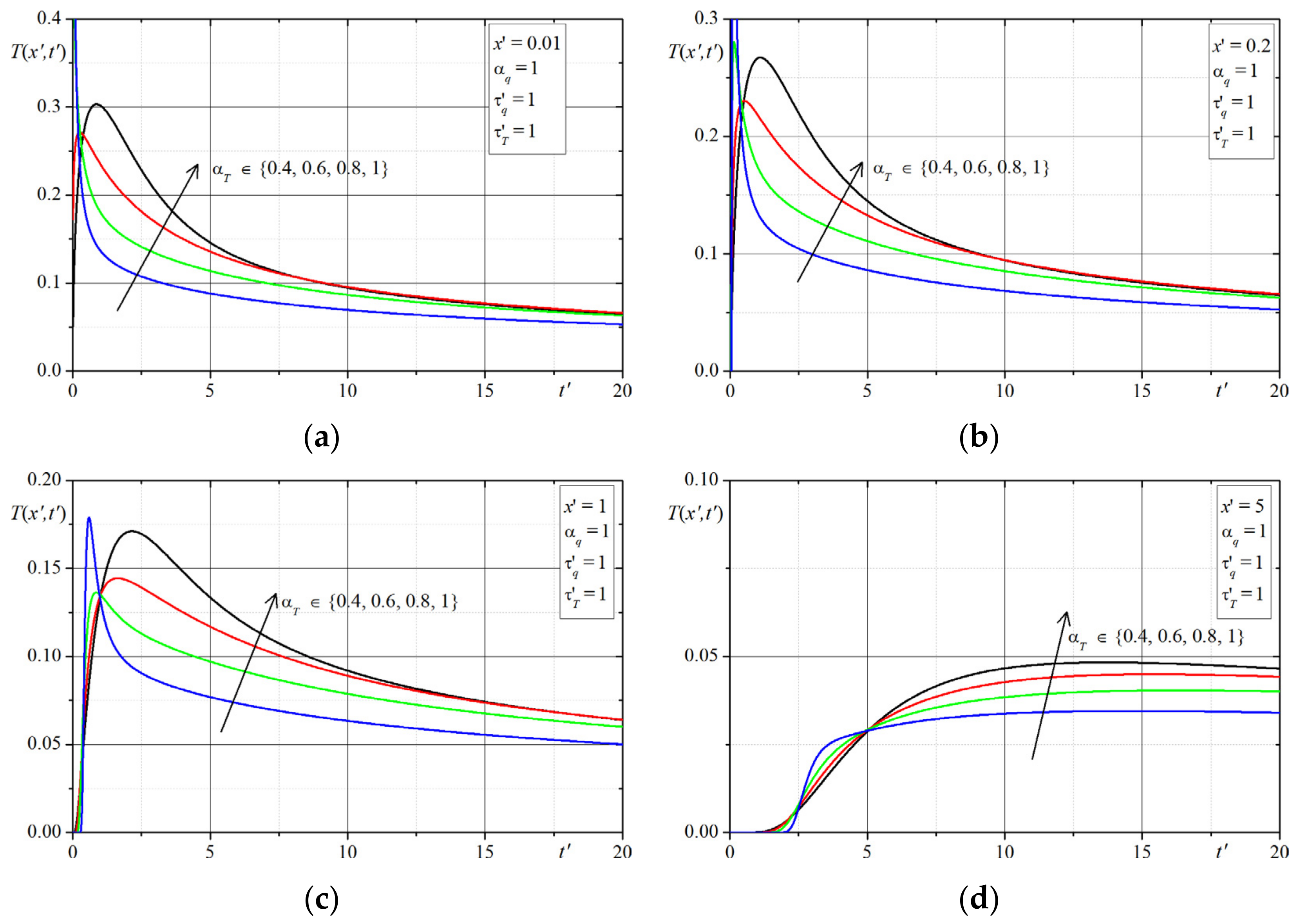
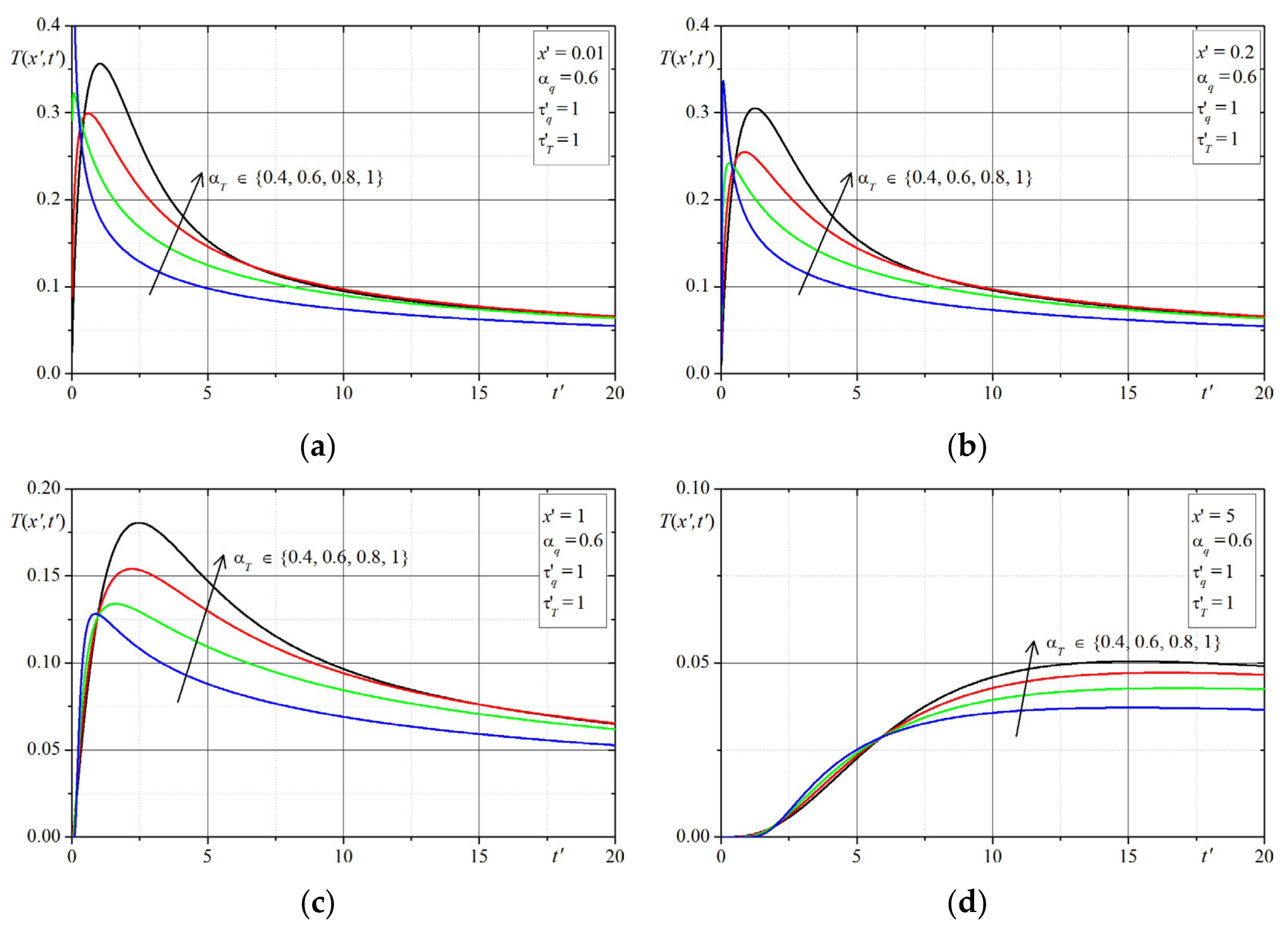
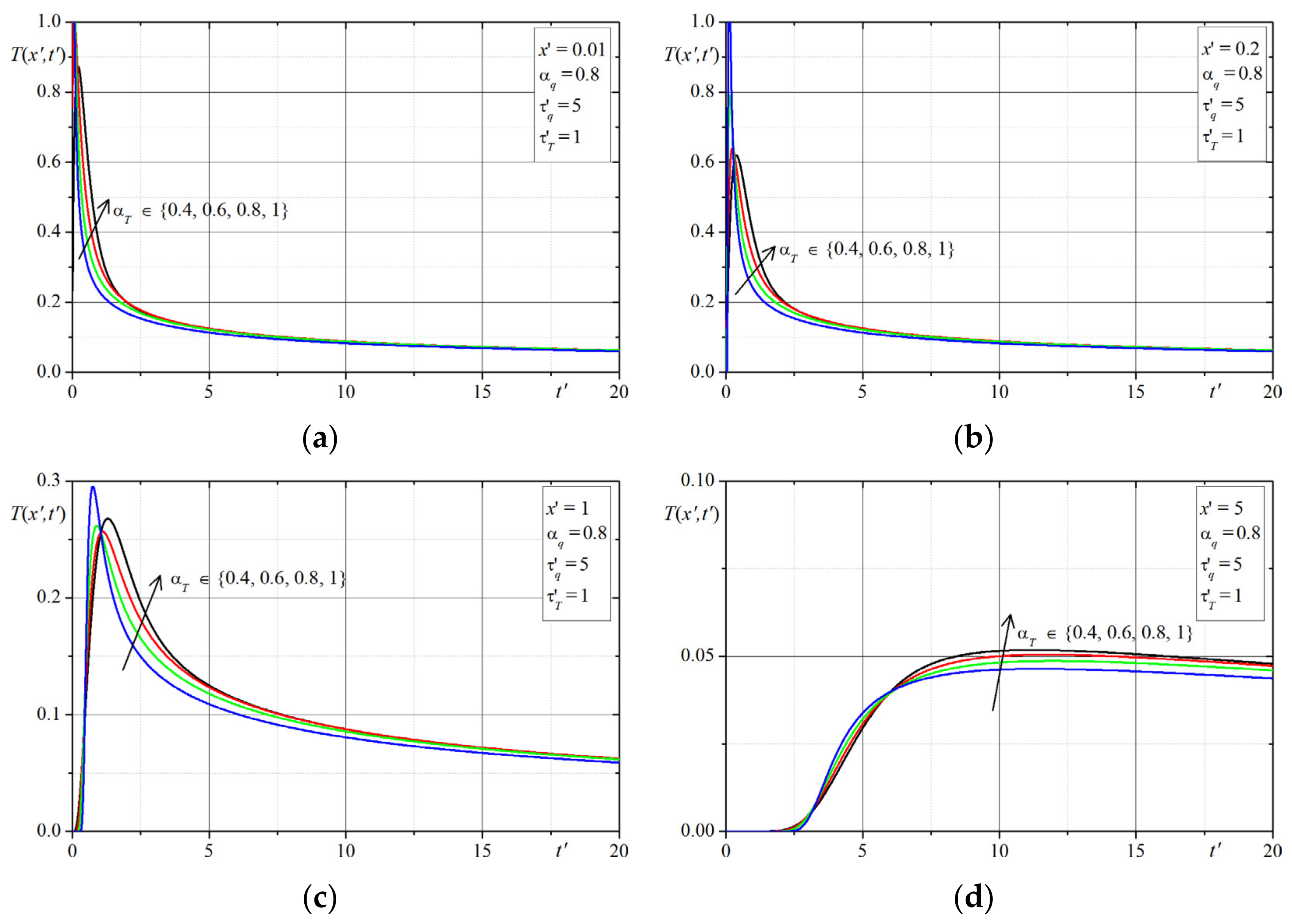
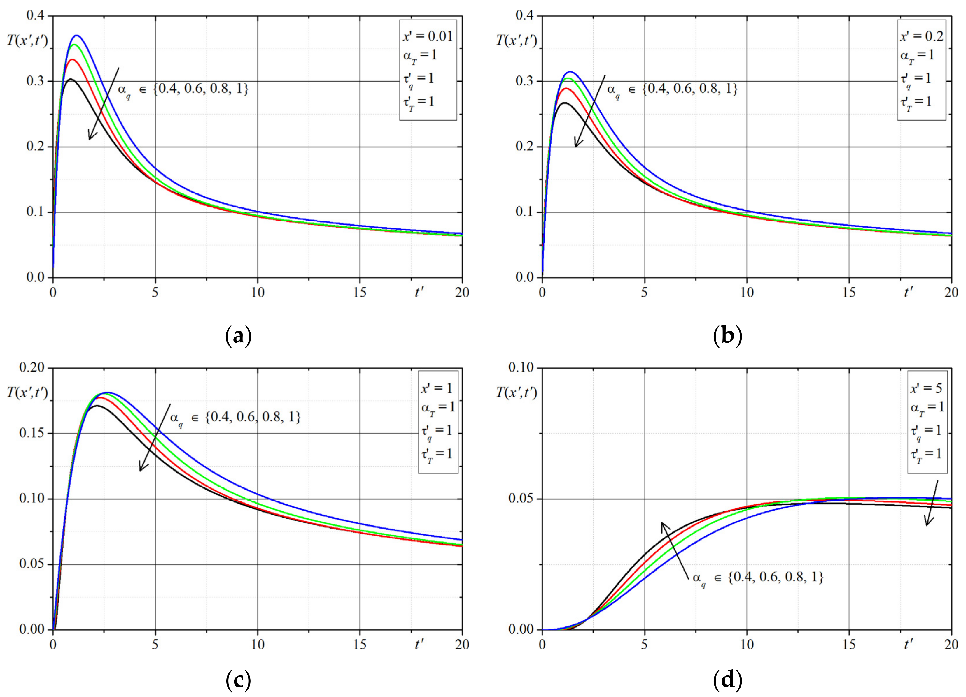
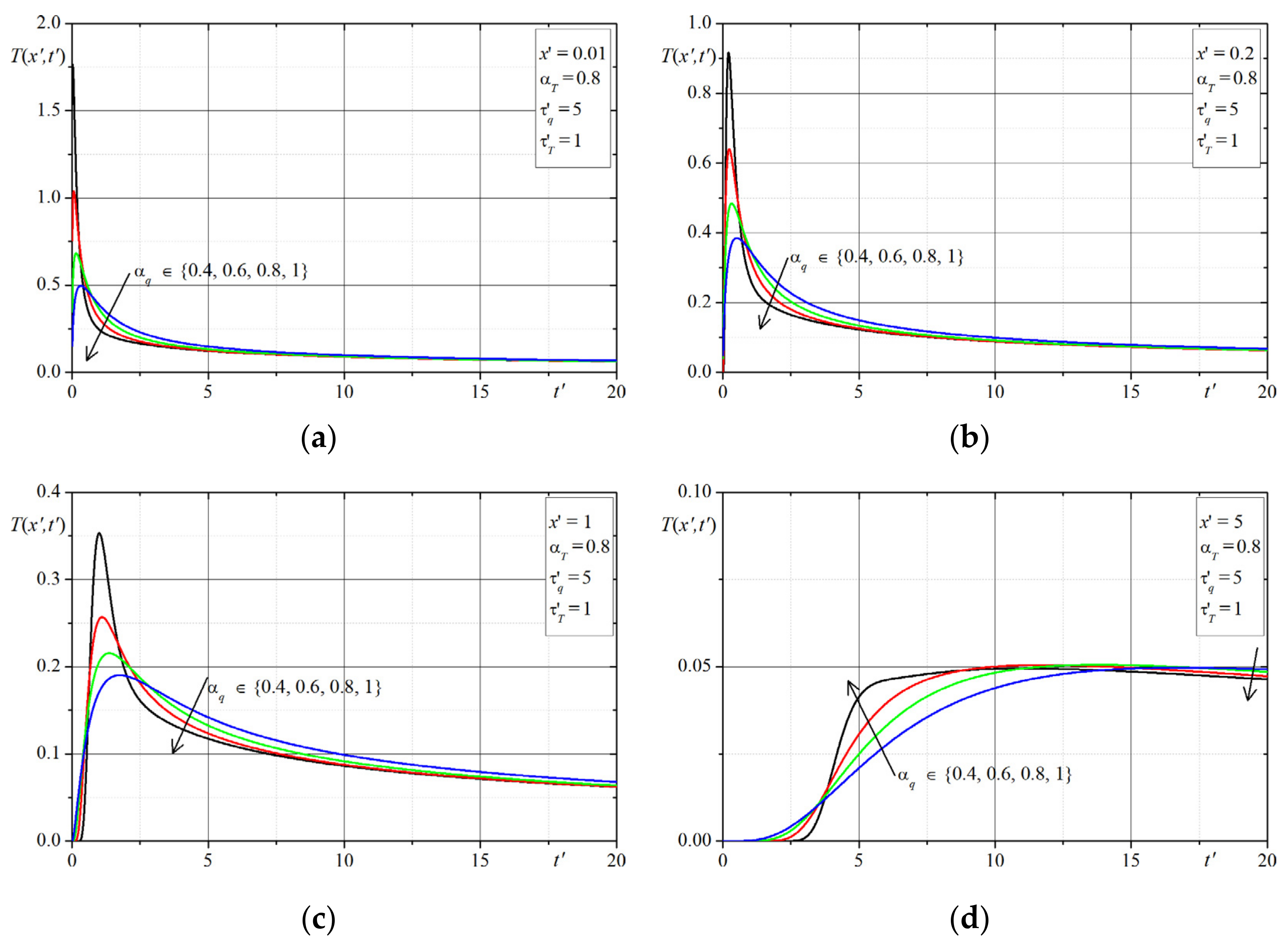
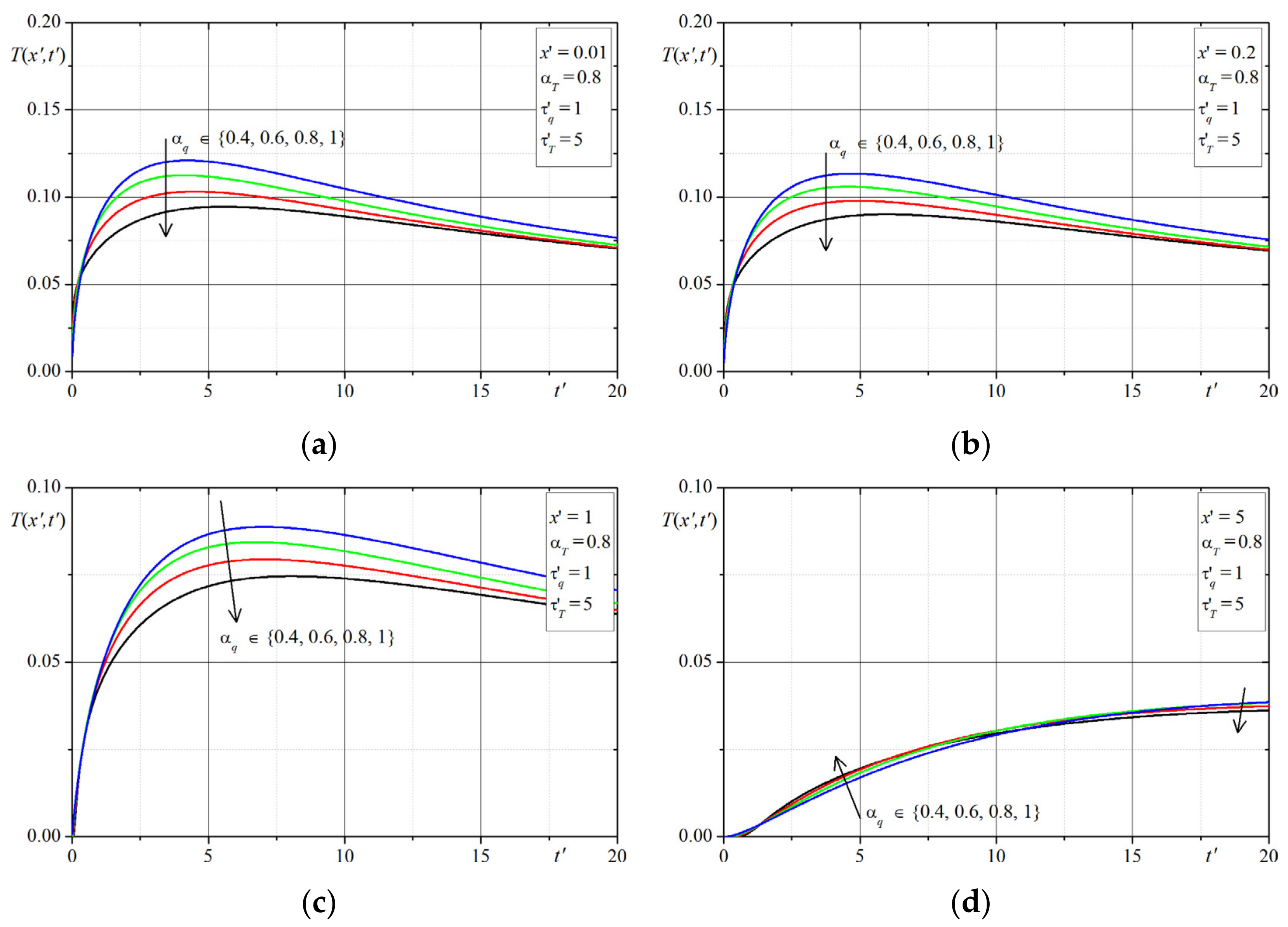
The solution presented in the Section 3, was be used to investigate the effect of the time-fractional order of the Caputo derivatives (${\mathsf{\alpha }}_T$ and ${\mathsf{\alpha }}_q$) as well as the phase-lag parameters (${{\mathsf{\tau }}^{\prime }}_T$ and ${{\mathsf{\tau }}^{\prime }}_q$) on the temperature distribution in the 1D domain. Two examples are presented. Note that the numerical calculations in all examples were performed for the non-dimensional variables given by Equations (20)–(23).

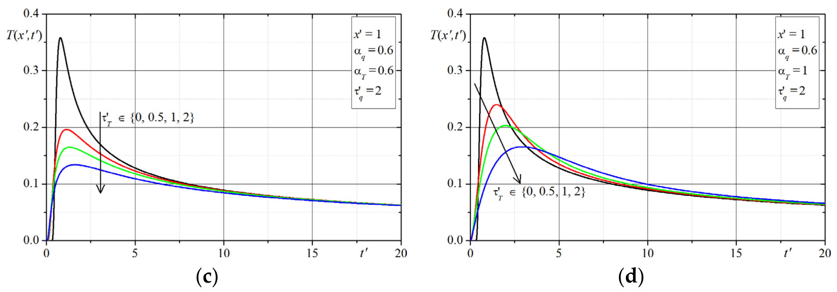
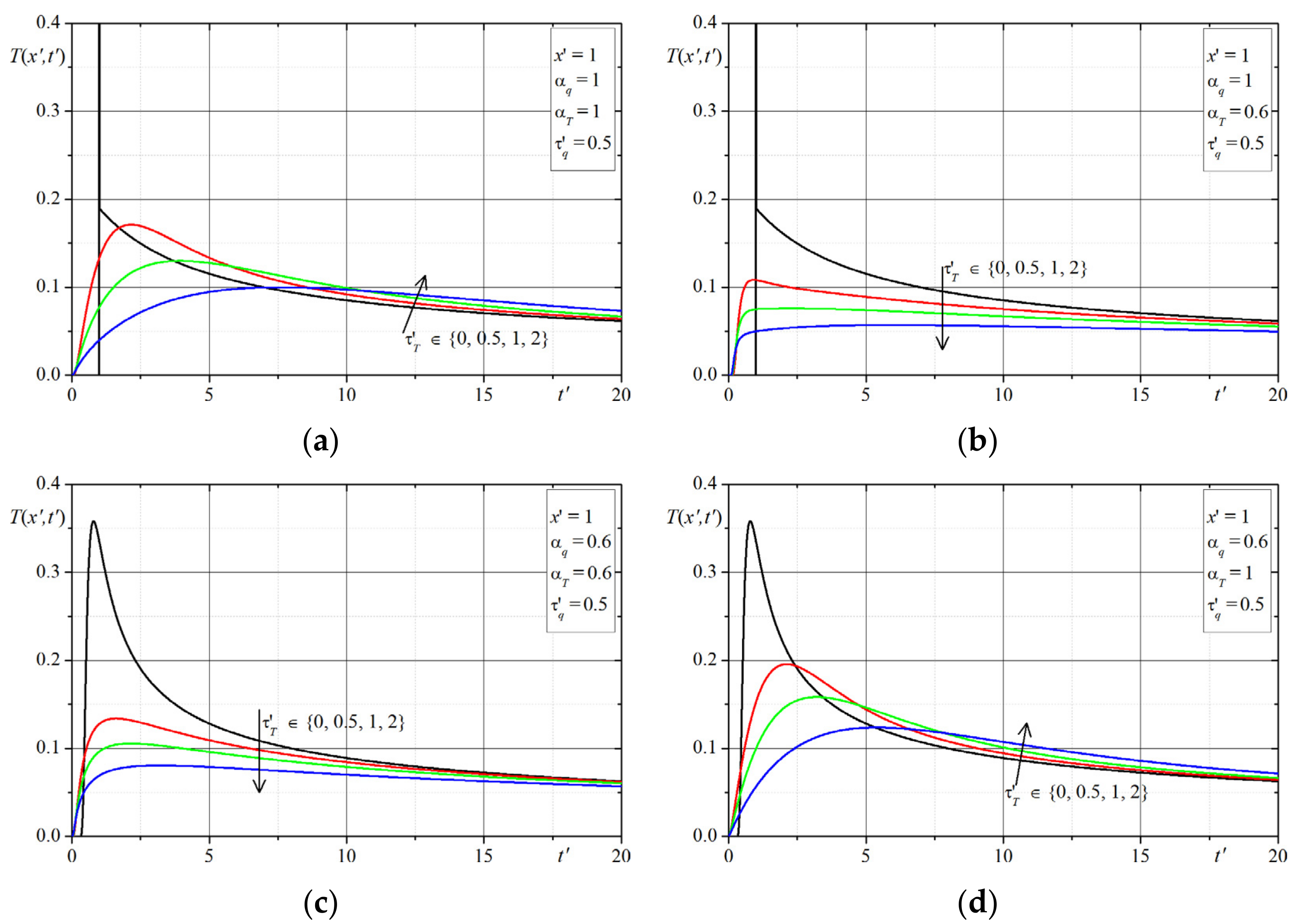
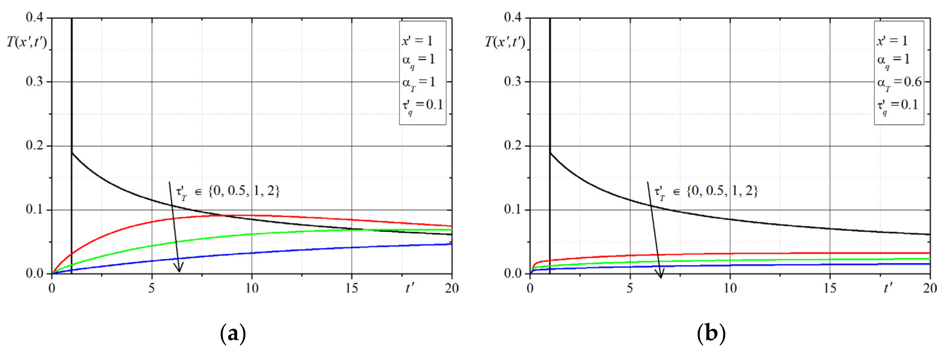
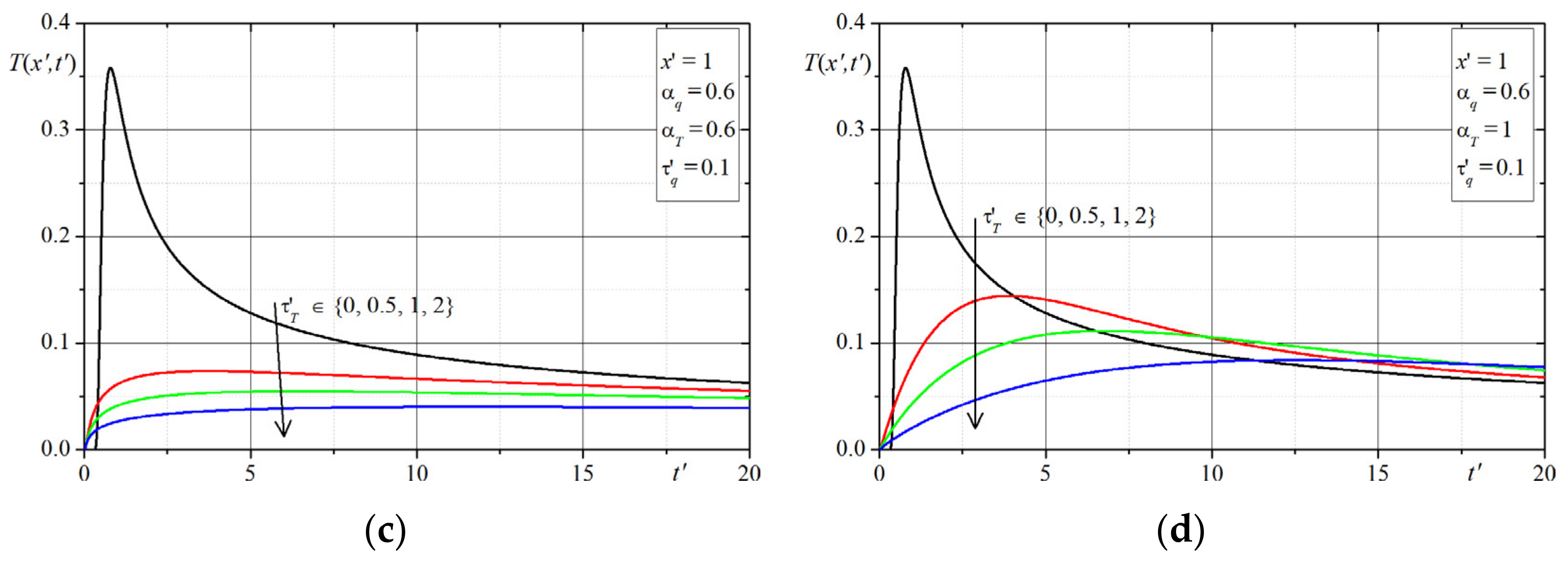
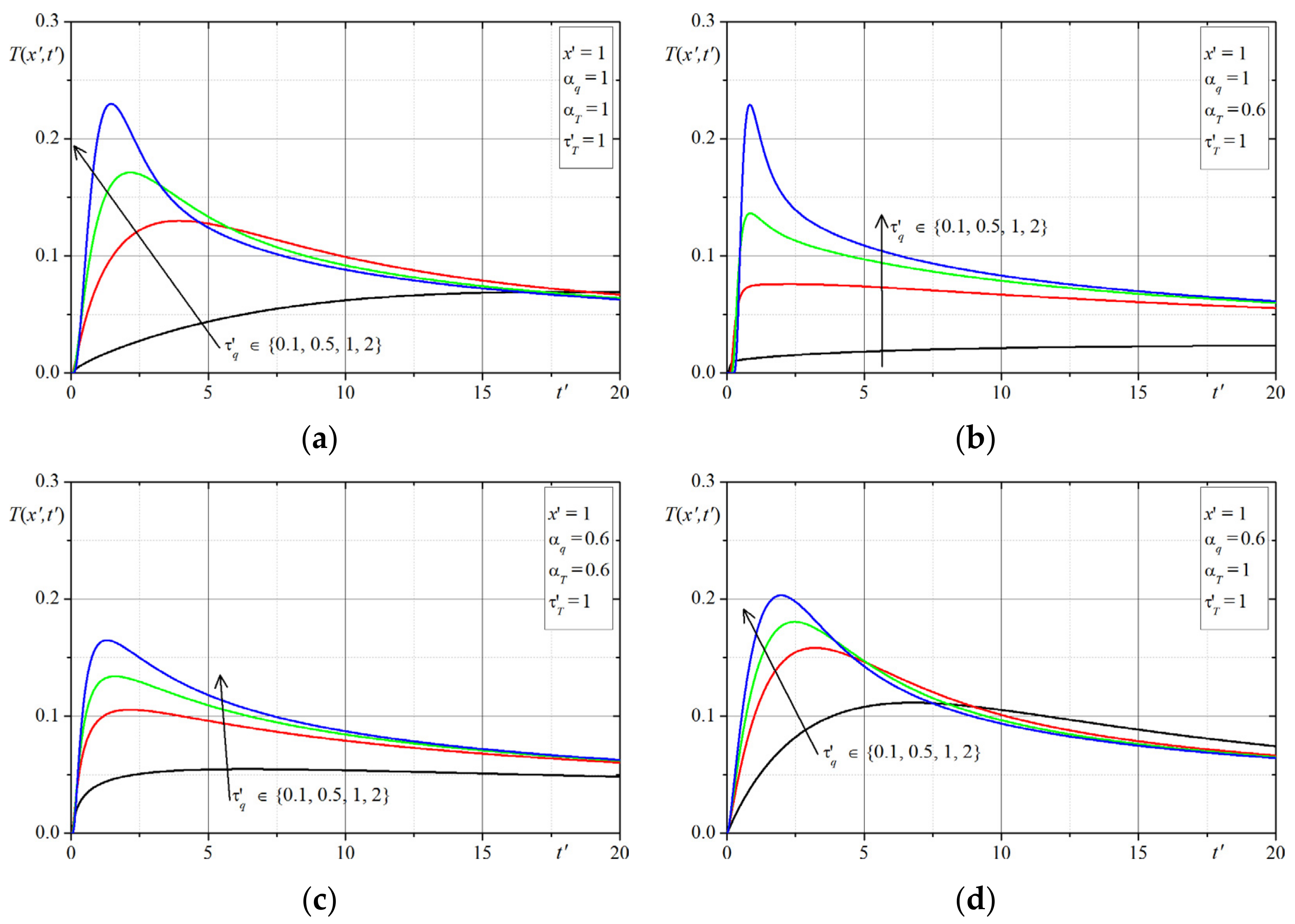
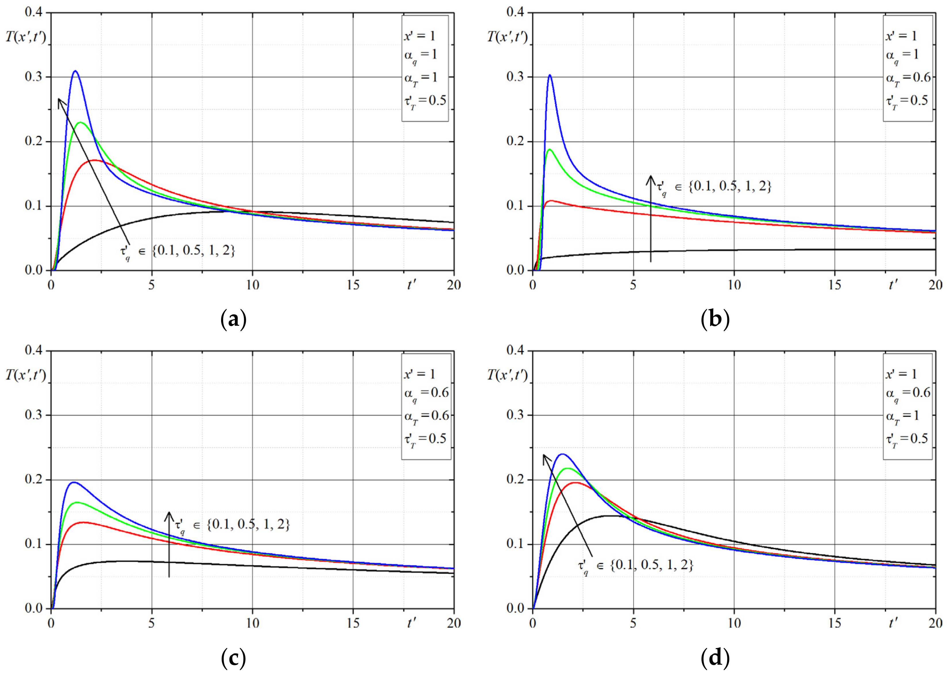
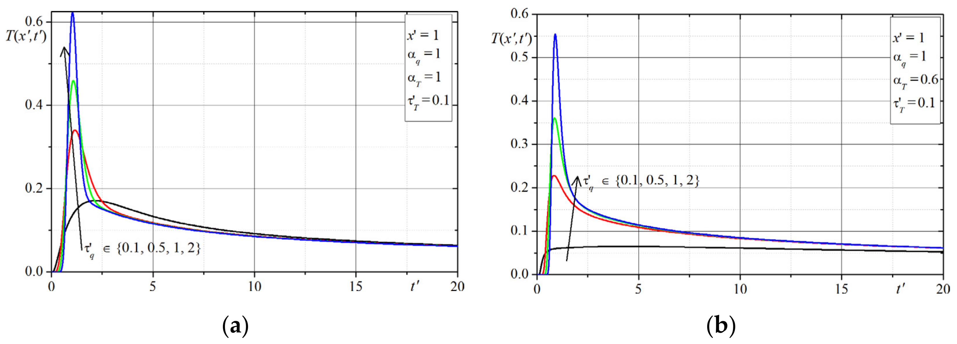
The first example concerns the effect of the time-fractional order of the both Caputo derivatives on the temperature distribution. The time-history’s temperatures in selected points $x^{\prime }$ are presented in Figure 1, Figure 2, Figure 3, Figure 4, Figure 5, Figure 6, Figure 7 and Figure 8. The graphs in each figure are done for fixed values of lags parameters ${{\mathsf{\tau }}^{\prime }}_T$, ${{\mathsf{\tau }}^{\prime }}_q$ and for: fixed values of order ${\mathsf{\alpha }}_q$ and various values of order ${\mathsf{\alpha }}_T$ (Figure 1, Figure 2, Figure 3 and Figure 4) or fixed values of order ${\mathsf{\alpha }}_T$ and various values of order ${\mathsf{\alpha }}_q$ (Figure 5, Figure 6, Figure 7 and Figure 8).

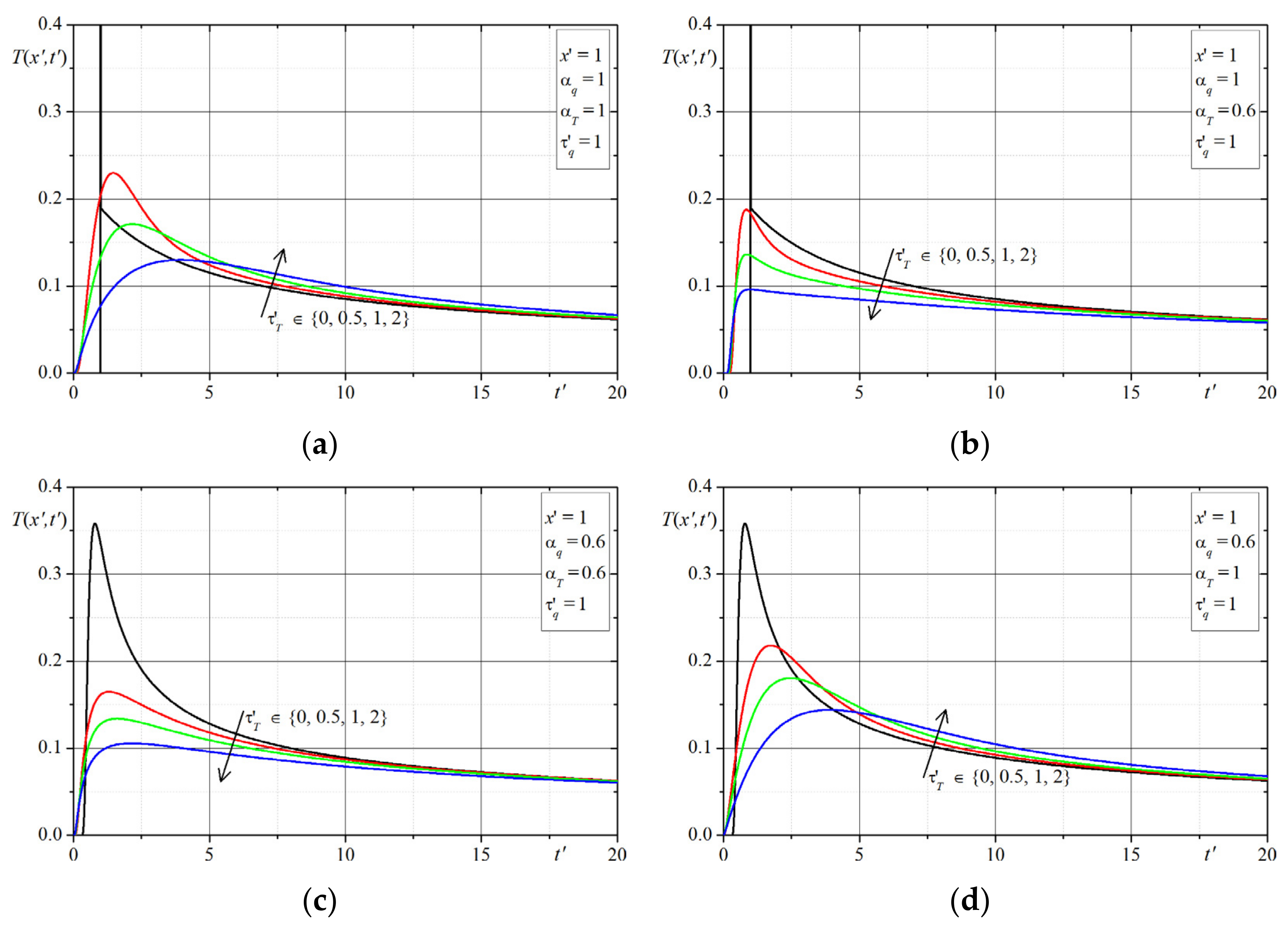
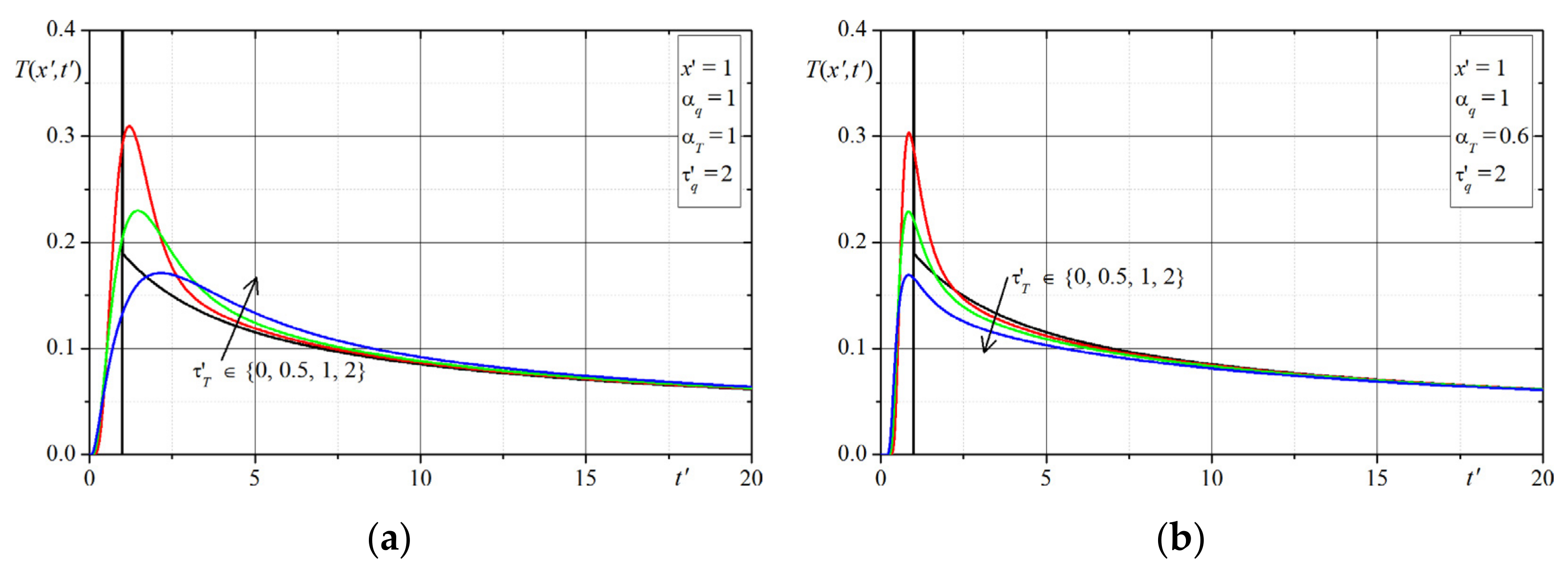
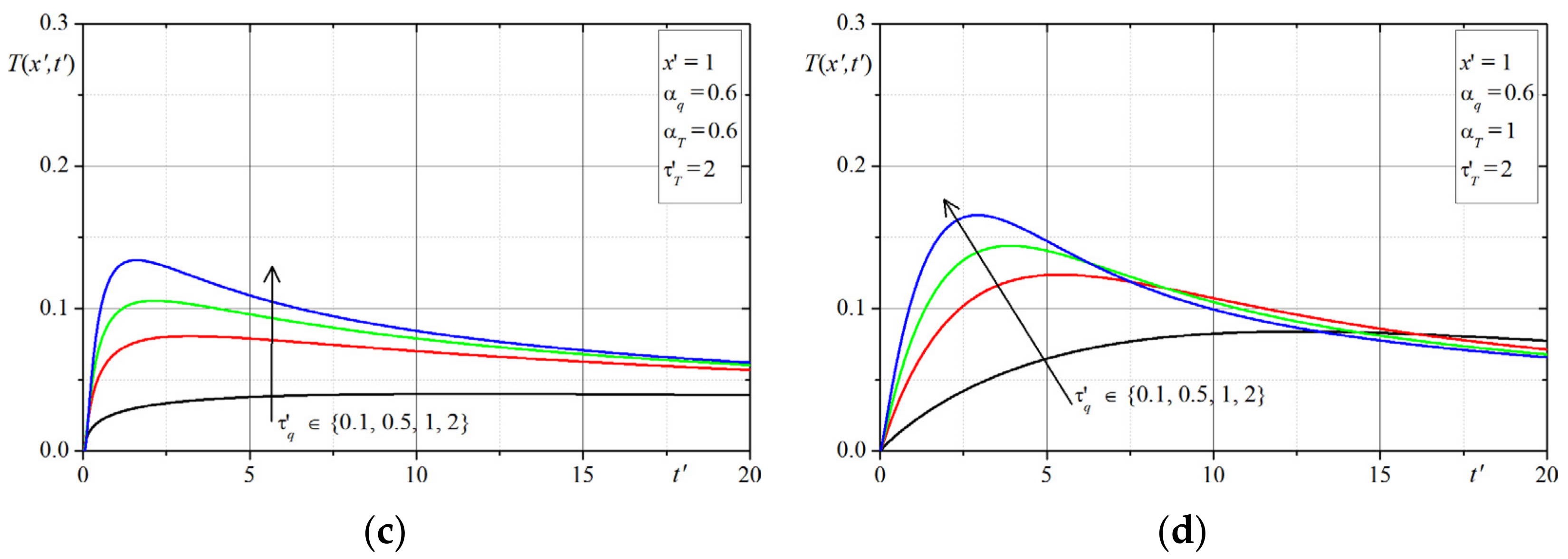
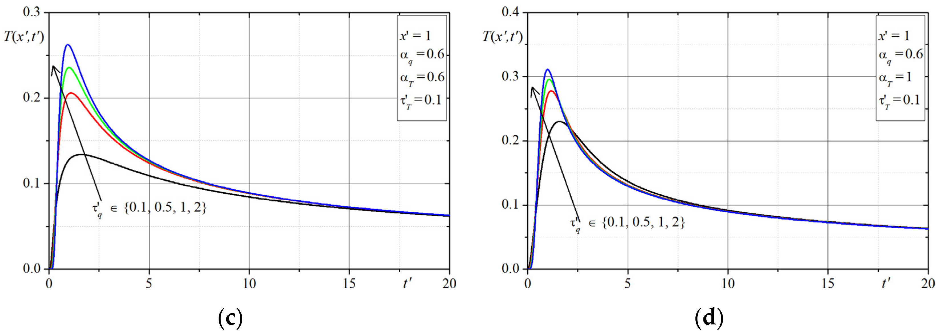
In the second example, there is a numerical investigation presented of the effect of lag parameters on distribution of temperature. The changes of temperature are analyzed for selected orders ${\mathsf{\alpha }}_T$ and ${\mathsf{\alpha }}_q$ in Figure 9, Figure 10, Figure 11, Figure 12, Figure 13, Figure 14 and Figure 15. The graphs presented in each figure are done for fixed points $x^{\prime }$ and for: fixed values of lag parameter ${{\mathsf{\tau }}^{\prime }}_q$ and various values of lag parameter ${{\mathsf{\tau }}^{\prime }}_T$ (Figure 9, Figure 10, Figure 11 and Figure 12) or fixed values of lag parameter ${{\mathsf{\tau }}^{\prime }}_T$ and various values of lag parameter ${{\mathsf{\tau }}^{\prime }}_q$ (Figure 13, Figure 14, Figure 15 and Figure 16).

Remarks on Solutions: In the presented examples, the cases of solutions for ${{\mathsf{\tau }}^{\prime }}_q=0$ have been omitted (the considered Equation (16) for ${{\mathsf{\tau }}^{\prime }}_q=0$ becomes the parabolic type equation and its solution takes on another special form). Assuming ${{\mathsf{\tau }}^{\prime }}_T=0$ then the parameter B = 0 and hence the solutions $T\left(x^{\prime },t^{\prime }\right)$ in dimensionless variables do not depend on the values of parameter ${{\mathsf{\tau }}^{\prime }}_q$. It can be seen in the above plots, that in the solutions for ${{\mathsf{\tau }}^{\prime }}_T=0$ and ${\mathsf{\alpha }}_q=1$ (this case corresponds to the classical Cattaneo equation), the characteristics peaks (the Dirac delta) are at the front of the thermal wave (considering the assumed initial conditions here). Analyzing all of the solutions presented in the plots (i.e., the changes of temperature in time at selected points of domain were determined depending on 4 parameters: ${{\mathsf{\tau }}^{\prime }}_T,{{\mathsf{\tau }}^{\prime }}_q,{\mathsf{\alpha }}_T,{\mathsf{\alpha }}_q$), one can conclude that the largest differences in the course of solutions (temperatures) occur in the initial period of time $t^{\prime }$, while if $t^{\prime }\to \infty$ then the differences resulting from the influence of the parameters ${{\mathsf{\tau }}^{\prime }}_T,{{\mathsf{\tau }}^{\prime }}_q,{\mathsf{\alpha }}_T,{\mathsf{\alpha }}_q$ disappear. In order to verify the correctness of the solutions for the given initial conditions, we additionally determined numerically the value of integral which should be equal to ${\displaystyle {\int }_{-\infty }^{\infty }T\left(x^{\prime },t^{\prime }\right)d{x}^{\prime }}=1$ for $t^{\prime }\ge 0$ and this property was satisfied in all cases for the parameters.

5. Conclusions

In this work, the fractional model of heat conduction has been presented. This model can be regarded as a generalization of the classical DPLM in which two additional parameters ${\mathsf{\alpha }}_q\in (0,1]$ and ${\mathsf{\alpha }}_T\in (0,1]$ are present. The fractional model allows one to obtain new feature solutions. A fundamental solution (also known as full-space Green’s function) of the fractional dual-phase-lag heat conduction problem was derived and presented. The Cauchy problem (in a whole-space domain) to the 1D FDPL equation was considered. The symmetry in the initial data (here expressed by the Dirac delta function) is carried through to the same symmetry in the fundamental solution about the point x = 0. The time-fractional differential equation was solved by using the Fourier–Laplace transform technique. The numerical calculations were performed by using the method which is based on the Fourier-series quadrature-type approximation to the Bromwich contour integral. Computational examples aimed to investigate the effect of the time-fractional derivative order and the phase-lag parameters on the temperature distribution. The fundamental solution has to do with bounded domains, where different Green’s functions must be found. A useful trick is to use symmetry to construct such Green’s functions on a semi-infinite domain from the derived Green’s function on the whole domain (this method is often called the method of images).

References

- Kilbas, A.A.; Srivastava, H.M.; Trujillo, J.J. Theory and Applications of Fractional Differential Equations. North-Holland Mathematical Studies; Elsevier (North-Holland) Science Publishers: Amsterdam, The Netherlands, 2006; Volume 204. [Google Scholar]
- Mainardi, F. Fractional Calculus and Waves in Linear Viscoelasticity: An Introduction to Mathematical Models; Imperial College Press: London, UK, 2010. [Google Scholar]
- Machado, J.A.T.; Silva, M.F.; Barbosa, R.S.; Jesus, I.S.; Reis, C.M.; Marcos, M.G.; Galhano, A. Some Applications of Fractional Calculus in Engineering. Math. Probl. Eng. 2010, 2010, 639801. [Google Scholar] [CrossRef] [Green Version]
- Sun, H.; Zhang, Y.; Baleanu, D.; Chen, W.; Chen, Y. A new collection of real world applications of fractional calculus in science and engineering. Commun. Nonlinear Sci. Numer. Simul. 2018, 64, 213–231. [Google Scholar] [CrossRef]
- Sierociuk, D.; Dzielinski, A.; Sarwas, G.; Petras, I.; Podlubny, I.; Skovranek, T. Modelling heat transfer in heterogeneous media using fractional calculus. Philos. Trans. R. Soc. 2013, 371, 146. [Google Scholar] [CrossRef] [PubMed] [Green Version]
- Žecová, M.; Terpak, J. Heat conduction modeling by using fractional-order derivatives. Appl. Math. Comput. 2015, 257, 365–373. [Google Scholar] [CrossRef] [Green Version]
- Majchrzak, E.; Mochnacki, B. Implicit scheme of the finite difference method for 1D dual-phase lag equation. J. Appl. Math. Comput. Mech. 2017, 16, 37–46. [Google Scholar] [CrossRef] [Green Version]
- Xu, H.-Y.; Jiang, X.-Y. Time fractional dual-phase-lag heat conduction equation. Chin. Phys. B 2015, 2015, 034401. [Google Scholar] [CrossRef]
- Ciesielski, M. Analytical solution of the dual phase lag equation describing the laser heating of thin metal film. J. Appl. Math. Comput. Mech. 2017, 16, 33–40. [Google Scholar] [CrossRef] [Green Version]
- Duffy, D.G. Green’s Functions with Applications; Chapman&Hall/CRC: Washington, DC, USA, 2001. [Google Scholar]
- Kukla, S. Green’s Functions and Its Applications; The Publishing Office of Czestochowa University of Technology: Czestochowa, Poland, 2009. (In Polish) [Google Scholar]
- Beck, J.V.; Cole, K.D.; Haji-Sheikh, A.; Litkouhi, B. Heat Conduction Using Green’s Functions; Hemisphere: Washington, DC, USA, 1992. [Google Scholar]
- Hahn, D.; Özişik, M.N. Heat Conduction; Wiley: New York, NY, USA, 2012. [Google Scholar]
- Kukla, S.; Siedlecka, U. Laplace transform solution of the problem of time-fractional heat conduction in a two-layered slab. J. Appl. Math. Comput. Mech. 2015, 14, 105–113. [Google Scholar] [CrossRef] [Green Version]
- Podlubny, I. Fractional Differential Equations; Academic Press: San Diego, CA, USA, 1999. [Google Scholar]
- Avci, D.; Yavuz, M.; Ozdemir, N. Fundamental Solutions to the Cauchy and Dirichlet Problems for a Heat Conduction Equation Equipped with the Caputo-Fabrizio Differentiation, in Book: Heat Conduction: Methods, Applications and Research; Nova Science Publishers: New York, NY, USA, 2019. [Google Scholar]
- Odibat, Z.M.; Shawagfeh, N.T. Generalized Taylor’s formula. Appl. Math. Comput. 2007, 186, 286–293. [Google Scholar] [CrossRef]
- Dyke, P. An Introduction to Laplace Transforms and Fourier Series; Springer: Berlin/Heidelberg, Germany, 2001. [Google Scholar]
- Gorenflo, R.; Kilbas, A.A.; Mainardi, F.; Rogosin, S.V. Mittag-Leffler Functions, Related Topics and Applications; Springer: Berlin/Heidelberg, Germany, 2014. [Google Scholar]
- De Hoog, F.R.; Knight, J.; Stokes, A.N. An Improved Method for Numerical Inversion of Laplace Transforms. SIAM J. Sci. Stat. Comput. 1982, 3, 357–366. [Google Scholar] [CrossRef]
Figure 1.
Temperature distribution for , , , and: (a) , (b) , (c) , (d) .
Figure 2.
Figure 3.
Figure 4.
Figure 5.
Figure 6.
Figure 7.
Figure 8.
Figure 9.
Temperature distribution for , , and: (a) , , (b) , , (c) , , (d) , .
Figure 10.
Figure 11.
Figure 12.
Figure 13.
Figure 14.
Figure 15.
Figure 16.
Publisher’s Note: MDPI stays neutral with regard to jurisdictional claims in published maps and institutional affiliations. |
© 2021 by the authors. Licensee MDPI, Basel, Switzerland. This article is an open access article distributed under the terms and conditions of the Creative Commons Attribution (CC BY) license (https://creativecommons.org/licenses/by/4.0/).
Share and Cite
MDPI and ACS Style
Ciesielski, M.; Siedlecka, U. Fractional Dual-Phase Lag Equation—Fundamental Solution of the Cauchy Problem. Symmetry 2021, 13, 1333. https://0-doi-org.brum.beds.ac.uk/10.3390/sym13081333
AMA Style
Ciesielski M, Siedlecka U. Fractional Dual-Phase Lag Equation—Fundamental Solution of the Cauchy Problem. Symmetry. 2021; 13(8):1333. https://0-doi-org.brum.beds.ac.uk/10.3390/sym13081333
Chicago/Turabian StyleCiesielski, Mariusz, and Urszula Siedlecka. 2021. "Fractional Dual-Phase Lag Equation—Fundamental Solution of the Cauchy Problem" Symmetry 13, no. 8: 1333. https://0-doi-org.brum.beds.ac.uk/10.3390/sym13081333
Note that from the first issue of 2016, this journal uses article numbers instead of page numbers. See further details here.