Quantum Particle on Dual Weight Lattice in Weyl Alcove

Abstract

Families of discrete quantum models that describe a free non-relativistic quantum particle propagating on rescaled and shifted dual weight lattices inside closures of Weyl alcoves are developed. The boundary conditions of the presented discrete quantum billiards are enforced by precisely positioned Dirichlet and Neumann walls on the borders of the Weyl alcoves. The amplitudes of the particle’s propagation to neighbouring positions are determined by a complex-valued dual-weight hopping function of finite support. The discrete dual-weight Hamiltonians are obtained as the sum of specifically constructed dual-weight hopping operators. By utilising the generalised dual-weight Fourier–Weyl transforms, the solutions of the time-independent Schrödinger equation together with the eigenenergies of the quantum systems are exactly resolved. The matrix Hamiltonians, stationary states and eigenenergies of the discrete models are exemplified for the rank two cases $C_2$ and $G_2$.

1. Introduction

The goal of this article is to assemble families of tight-binding models [1,2,3] by describing a free non-relativistic quantum particle which propagates on shifted and rescaled dual weight lattices inside closures of scaled Weyl alcoves. Similarly to the recently developed dual-root lattice models [1], the boundary conditions of the presented discrete quantum billiards [4,5] are enforced by precisely positioned Dirichlet and Neumann walls.

The quantum billiard systems of multiform shapes that include 2D stadium [6], Hecke triangular domains [7], equilateral triangle on a spherical surface [8] and polygons [9] have been investigated. The quantum billiards on 2D triangles [10,11,12] and 3D Weyl chamber [13] realise the closest versions of the current simplex-shaped models. From the viewpoint of position restrictions, the discrete quantum billiards [4,14] involve the propagating particle on quantum dots [15,16,17]. Single particle properties of the quantum dots are commonly studied via the discrete tight-binding Hamiltonians [3,15,17]. Specifically for the studied class of tight-binding atomic lattice models [3,15], the atoms are coupled to neighbours of a predetermined fixed degree and possible overlaps among atom orbitals are neglected. The multivariate discrete Fourier transform provides a fundamental tool for deriving eigenenergies and momentum bases of these discrete tight-binding models. By utilising the underlying symmetries of the developed discrete quantum systems for implementing boundary conditions, it appears that generalised dual weight lattice Fourier–Weyl transforms [18,19,20] provide similarly crucial connections between position and momentum bases together with exact eigenenergies and time evolutions.

Representing a ubiquitous class of the discrete Fourier–Weyl transforms [21,22,23,24], the generalised dual-weight Fourier–Weyl transforms [18,19,20] form extensions of the classical trigonometric transforms [25] to the crystallographic root systems [26]. Symmetrised and signed by the actions of the Weyl groups together with the sign homomorphisms [27], the four types of Weyl orbit functions [19,20] that are characterised by labels from the weight lattices shifted by admissible shifts [18] serve as kernels of the generalised dual-weight and dual-root Fourier–Weyl transforms. The closure of the Weyl alcove, which forms an exactly determined simplex in the Euclidean space and represents a suitably chosen fundamental domain of the affine Weyl group, comprises the point sets of dual-weight Fourier–Weyl transforms. These point sets are determined as admissibly shifted dual weight lattices which are refined by a suitable magnifying factor and intersected with the signed fundamental domains of the affine Weyl groups [18]. The point sets of the dual-weight Fourier–Weyl transforms, which are scaled by a fixed length factor, represent discrete positions of the quantum particle inside the scaled closures of the Weyl alcoves. As demonstrated on the current $C_2$ models and the $C_2$ dual-root cases from [1], the relative positions of the point sets of the dual-weight lattice transforms with respect to the Weyl alcove essentially differ from the locations of the dual root lattice points. Thus, the collection of the discrete quantum models is substantially enhanced.

Common to both dual-weight and dual-root quantum systems, the faces of the signed fundamental domain inside the scaled closure of the Weyl alcove form the Neumann walls of perfect mirrors and the remaining boundaries constitute the Dirichlet walls of ideal barriers. Labelled by the point sets of the generalised dual-weight Fourier–Weyl transforms, the orthonormal position bases span the associated finite-dimensional Hilbert spaces of the quantum systems and represent the particle positioned at the given lattice point. The dual-weight coupling sets, which are attached to any two positions from the point sets, are utilised to characterise the hopping of the particle to neighbouring positions of a fixed degree along with action of the boundary walls via affine Weyl group orbits of the target positions. Finite sums of the dual-weight hopping operators [1] on the Hilbert spaces determine the final form of the discrete dual-weight tight-binding Hamiltonian [3] associated to each model. It appears that the normalised stationary state vectors, which represent solutions of the time-independent Schrödinger equation, are obtained by the inverse generalised dual-weight Fourier–Weyl transforms [18,19,20] of the orthonormal position bases. Moreover, the eigenenergies of the dual-weight quantum billiard systems are exactly calculated by adding together the symmetric Weyl orbit sums [28] corresponding to the chosen degree of coupling.

The developed dual-weight quantum models, together with their exact time-evolutions provided by the generalised dual-weight Fourier–Weyl transforms, produce a systematic method for description of a vast collection of discrete quantum billiard systems [1,4,5,14,17,29]. The presented dual-weight Fourier–Weyl methods of the rank two and three crystallographic root systems are anticipated to be applicable principally in analysis of electronic properties of 2D and 3D materials [30,31]. Both dual-weight and dual-root methods offer rigorous Hamiltonian treatment of the coupling between neighbouring lattice positions to any fixed degree [1]. Combining dual-root with dual-weight Fourier–Weyl transforms [18,19,20] and the corresponding quantum systems potentially produces Hamiltonian descriptions of the $A_2$ triangular graphene quantum dots [15,17] together with the $A_3$ tetrahedral diamond structures [32]. Furthermore, the developed discrete quantum models potentially serve as a foundation for the description of quantum field lattice models [32], ultracold atoms in optical lattices [33], dynamics of particles in potential traps with interactions [34], quantum gates [13], discrete space-time models [35] and quantum waveguides [36].

This paper is organised as follows. In Section 2, the prerequisite facts concerning the root systems, affine Weyl groups, $\chi$-function and Weyl orbit functions are outlined. Section 3 is dedicated to the description of the dual-weight hopping function and hopping operators, discrete Hamiltonians and time evolution of the proposed quantum systems. In Section 4, examples of the dual-weight models with the implemented nearest and next-to-nearest coupling are presented for the root systems $C_2$ and $G_2$. Comments and follow-up questions are included in the last section.

2. Dual-Weight Fourier–Weyl Transforms

2.1. Weyl Groups and Invariant Shifted Lattices

The mathematical exposition and notations of this article are established in papers [19,20,21,22]. Each simple Lie algebra from the classical four series $A_n(n\ge 1)$, $B_n(n\ge 3)$, $C_n(n\ge 2)$ and $D_n(n\ge 4)$ and from the five exceptional cases $E_6,E_7,E_8,F_4,G_2$ determines the set $\Delta =\{{\alpha }_1,\dots ,{\alpha }_n\}$ of the simple roots [37,38]. For the simple Lie algebras $B_n,C_n,F_4$ and $G_2$, the set $\Delta$ is disjointly decomposed into the set ${\Delta }_s$ of the short simple roots and the set ${\Delta }_l$ of the long simple roots,

$$\Delta ={\Delta }_s\cup {\Delta }_l.$$

(1)

The vectors of the set $\Delta$ span the Euclidean space ${\mathbb{R}}^n$ equipped with the standard scalar product $〈·,·〉$. The simple roots ${\alpha }_i$, $i\in \{1,\dots ,n\}$, rescaled by the length factor $2/〈{\alpha }_i,{\alpha }_i〉$, produce the set ${\Delta }^{\vee }$ of dual simple roots ${\alpha }_i^{\vee }$. The dual basis for the basis of simple roots $\Delta$ is formed by dual fundamental weights ${\omega }_i^{\vee }$, which are given by $〈{\omega }_i^{\vee },{\alpha }_j〉={\delta }_{ij}$, $i,j\in \{1,\dots ,n\}$, and the dual basis corresponding to the basis of the dual simple roots ${\Delta }^{\vee }$ consists of fundamental weights ${\omega }_i$ satisfying $\langle {\omega }_i,{\alpha }_j^{\vee }\rangle ={\delta }_{ij}$.

The reflection $r_i$, associated to each simple root ${\alpha }_i\in \Delta$, is specified by the following standard formula,

$$r_{i}a=a-〈a,{\alpha }_i^{\vee }〉{\alpha }_i,a\in {\mathbb{R}}^n.$$

The reflections $r_i,i\in \{1,\dots ,n\}$ generate the finite Weyl group $W.$ The action of the Weyl group W on the set of simple roots $\Delta$ produces the entire root system $\Pi =W\Delta$ which contains a unique highest root $\xi \in \Pi$ of the following form,

$$\xi =m_1{\alpha }_1+\cdots +m_n{\alpha }_n.$$

The set of dual simple roots ${\Delta }^{\vee }$ induces via the Weyl group action the entire dual root system ${\Pi }^{\vee }=W{\Delta }^{\vee }$ that includes the highest dual root of the following form,

$$\eta =m_1^{\vee }{\alpha }_1^{\vee }+\cdots +m_n^{\vee }{\alpha }_n^{\vee }.$$

The marks of the highest root $m_1,\dots ,m_n$ and the dual marks of the highest dual root $m_1^{\vee },\dots ,m_n^{\vee }$ are summarised in Table 1 in [20].

The opposite involution $w_0\in W$ that is uniquely associated to each set of simple roots $\Delta$ attains for the types $A_1$, $B_n(n\ge 3)$, $C_n(n\ge 2)$, $D_{2k}(k\ge 2)$, $E_7$, $E_8$, $F_4$, $G_2$ the form of the negative identity, $w_0=-1.$ The opposite involutions of the remaining cases [37] are obtained, by expressing any vector $a\in {\mathbb{R}}^n$ in the ${\omega }^{\vee }$-basis:

$$a=a_1{\omega }_1^{\vee }+\cdots +a_n{\omega }_n^{\vee }=(a_1,\dots ,a_n),$$

as follows,

$$\begin{array}{cc}\hfill A_n(n\ge 2):& w_0(a_1,a_2,\dots ,a_n)=-(a_n,a_{n-1},\dots ,a_1),\hfill \\ \hfill D_{2k+1}(k\ge 2):& w_0(a_1,a_2,\dots ,a_{2k-1},a_{2k},a_{2k+1})=-(a_1,a_2,\dots ,a_{2k-1},a_{2k+1},a_{2k}),\hfill \\ \hfill E_6:& w_0(a_1,a_2,a_3,a_4,a_5,a_6)=-(a_5,a_4,a_3,a_2,a_1,a_6).\hfill \end{array}$$

(2)

Any homomorphism $\sigma :W\to U_2$ from the Weyl group W to the multiplicative group $U_2=\{\pm 1\}$ is called a sign homomorphism [19]. The identity $\mathfrak{1}$ and the determinant ${\sigma }^e$ sign homomorphisms are, for any Weyl group $W,$ defined on the generating reflections $r_i$ as follows,

$$\begin{array}{cc}\hfill \mathfrak{1}\left(r_i\right)& =-{\sigma }^e\left(r_i\right)=1.\hfill \end{array}$$

For the sets $\Delta$ with two root-lengths (1), the short ${\sigma }^s$ and long ${\sigma }^l$ sign homomorphisms are determined on the generating reflections $r_i$ as follows,

$$\begin{array}{cc}\hfill {\sigma }^s\left(r_i\right)=-{\sigma }^l\left(r_i\right)& =\left\{\begin{array}{cc}-1,\hfill & {\alpha }_i\in {\Delta }_s,\hfill \\ 1,\hfill & {\alpha }_i\in {\Delta }_l.\hfill \end{array}\right.\hfill \end{array}$$

Four classical Weyl group invariant lattices [37] comprise the root lattice Q, the dual weight lattice $P^{\vee }$, the dual root lattice $Q^{\vee }$ and the weight lattice P. These lattices are defined as the $\mathbb{Z}$-spans of the following basis vectors of ${\mathbb{R}}^n$,

$$\begin{array}{cccc}& Q\hfill & \hfill =& \mathbb{Z}{\alpha }_1+\cdots +\mathbb{Z}{\alpha }_n,\hfill \\ & P^{\vee }\hfill & \hfill =& \mathbb{Z}{\omega }_1^{\vee }+\cdots +\mathbb{Z}{\omega }_n^{\vee },\hfill \\ & Q^{\vee }\hfill & \hfill =& \mathbb{Z}{\alpha }_1^{\vee }+\cdots +\mathbb{Z}{\alpha }_n^{\vee },\hfill \\ & P\hfill & \hfill =& \mathbb{Z}{\omega }_1+\cdots +\mathbb{Z}{\omega }_n.\hfill \end{array}$$

The dual weight lattice $P^{\vee }$ is $\mathbb{Z}$-dual to the root lattice Q, and the weight lattice is $\mathbb{Z}$-dual to the dual root lattice $Q^{\vee }$. The orders of the quotient groups $P/Q$ and $P^{\vee }/Q^{\vee }$ equal the determinant c of the Cartan matrix $C_{ij}=〈{\alpha }_i,{\alpha }_j^{\vee }〉,$

$$c=detC=\left|P/Q\right|=|P^{\vee }/Q^{\vee }|.$$

The cone of the positive dual weights $P^{\vee +}$ that comprises all points from the dual weight lattice $P^{\vee }$ in the fundamental Weyl chamber, is explicitly given as the following [37],

$$P^{\vee +}={\mathbb{Z}}^{\ge 0}{\omega }_1^{\vee }+\cdots +{\mathbb{Z}}^{\ge 0}{\omega }_n^{\vee }.$$

Since the fundamental Weyl chamber contains precisely one point of each W-orbit, the action of the Weyl group W on the cone $P^{\vee +}$ produces the entire lattice $P^{\vee }$ as follows,

$$W{P}^{\vee +}=P^{\vee }.$$

(3)

A vector $\varrho \in {\mathbb{R}}^n$, for which the Weyl group invariance condition holds as follows:

$$W(\varrho +P)=\varrho +P,$$

(4)

constitutes an admissible shift of the weight lattice [18]. Similarly, a vector ${\varrho }^{\vee }\in {\mathbb{R}}^n$, such that the following is the case:

$$W({\varrho }^{\vee }+P^{\vee })={\varrho }^{\vee }+P^{\vee },$$

(5)

represents an admissible shift of the dual weight lattice [18]. The equivalent admissible shifts induce identical shifted weight and dual weight lattices, respectively. The admissible shifts of the weight and dual weight lattices are listed up to equivalence in Table I of [18].

2.2. Signed Fundamental Domains

The affine Weyl group is the following semidirect product of the translation group $Q^{\vee }$ and the Weyl group W,

$$W^{\mathrm{aff}}=Q^{\vee }⋊W.$$

(6)

For any translation by the vector $q^{\vee }\in Q^{\vee }$ and any $w\in W,$ the affine Weyl group element $z=T\left(q^{\vee }\right)w\in W^{\mathrm{aff}}$ acts canonically on ${\mathbb{R}}^n$ as follows,

$$z·a=wa+q^{\vee },a\in {\mathbb{R}}^n.$$

The fundamental domain $F\subset {\mathbb{R}}^n$ of $W^{\mathrm{aff}}$, which contains exactly one point from each $W^{\mathrm{aff}}$-orbit, forms a simplex explicitly described by the following,

$$F=\left\{a_1{\omega }_1^{\vee }+\cdots +a_n{\omega }_n^{\vee }|a_0+m_1{a}_1+\cdots +m_n{a}_n=1,a_i\ge 0,i=0,\dots ,n\right\}.$$

The stabiliser ${\mathrm{Stab}}_{W^{\mathrm{aff}}}\left(a\right)$ is the subgroup of $W^{\mathrm{aff}}$ that comprises the elements stabilising $a\in {\mathbb{R}}^n$ and the associated discrete ${\epsilon }^{}-\mathrm{function}$ ε: ${\mathbb{R}}^n\to \mathbb{N}$ is defined by the following,

$$\epsilon \left(a\right)=\frac{\left|W\right|}{|{\mathrm{Stab}}_{W^{\mathrm{aff}}}\left(a\right)|}.$$

(7)

The algorithm for the calculation of the coefficients $\epsilon \left(a\right)$ is detailed in ([20], §3.7).

The retraction homomorphism $\psi :W^{\mathrm{aff}}\to W$ and the mapping $\tau :W^{\mathrm{aff}}\to Q^{\vee }$ are determined for any element $z=T\left(q^{\vee }\right)w\in W^{\mathrm{aff}}$ by the following relations,

$$\psi \left(z\right)=w,\tau \left(z\right)=q^{\vee }.$$

(8)

The mapping $\tau$ induces, for any admissible shift $\varrho$ of the weight lattice P, the dual shift homomorphism ${\theta }_{\varrho }:W^{\mathrm{aff}}\to U_2$ given in [18] as follows,

$${\theta }_{\varrho }\left(z\right)=e^{2\pi \mathrm{i}〈\tau \left(z\right),\varrho 〉}.$$

(9)

The dual shift homomorphism ${\theta }_{\varrho }$, restricted to the Weyl group W, evaluates as the following,

$${\theta }_{\varrho }\left(w\right)=1,w\in W.$$

(10)

For any sign homomorphism $\sigma$ and any admissible shift $\varrho$ of the weight lattice P, the homomorphism ${\gamma }_{\varrho }^{\sigma }:W^{\mathrm{aff}}\to U_2$ is built from the retraction and dual shift homomorphisms as the following product,

$${\gamma }_{\varrho }^{\sigma }\left(z\right)={\theta }_{\varrho }\left(z\right)[\sigma \circ \psi \left(z\right)].$$

(11)

The values of ${\gamma }_{\varrho }^{\sigma }$ on the generators of $W^{\mathrm{aff}}$ are listed in Table II in [18].

Since F is a fundamental domain of $W^{\mathrm{aff}}$, for any $a\in {\mathbb{R}}^n$ there exist exactly one point $a^{\prime }\in F$ and $z\left[a\right]\in W^{\mathrm{aff}}$ satisfying the following,

$$a=z\left[a\right]·a^{\prime }.$$

(12)

Employing relation (12), the function ${\chi }_{\varrho }^{\sigma }:{\mathbb{R}}^n\to \{-1,0,1\}$ is introduced in [1] for any $a\in {\mathbb{R}}^n$ by the following,

$${\chi }_{\varrho }^{\sigma }\left(a\right)=\left\{\begin{array}{cc}{\gamma }_{\varrho }^{\sigma }\left(z\left[a\right]\right),\hfill & {\gamma }_{\varrho }^{\sigma }\left({\mathrm{Stab}}_{W^{\mathrm{aff}}}\left(a\right)\right)=1,\hfill \\ 0,\hfill & {\gamma }_{\varrho }^{\sigma }\left({\mathrm{Stab}}_{W^{\mathrm{aff}}}\left(a\right)\right)=U_2.\hfill \end{array}\right.$$

(13)

To each sign homomorphism $\sigma$ and admissible shift $\varrho$ of the weight lattice corresponds a signed fundamental domain $F^{\sigma }\left(\varrho \right)\subset F$ given by the following,

$$F^{\sigma }\left(\varrho \right)=\left\{a\in F\mid {\chi }_{\varrho }^{\sigma }\left(a\right)=1\right\}.$$

(14)

In particular, it holds that $F^{\mathfrak{1}}\left(0\right)=F$ and $F^{{\sigma }^e}\left(0\right)=\mathrm{int}\left(F\right)$. Two subsets $H^{\sigma }\left(\varrho \right),B^{\sigma }\left(\varrho \right)\subset \partial F$ of the boundary $\partial F$ are described by the following,

$$\begin{array}{cc}\hfill H^{\sigma }\left(\varrho \right)& =\left\{a\in \partial F|{\chi }_{\varrho }^{\sigma }\left(a\right)=0\right\},\hfill \end{array}$$

(15)

$$\begin{array}{cc}\hfill B^{\sigma }\left(\varrho \right)& =\left\{a\in \partial F|{\chi }_{\varrho }^{\sigma }\left(a\right)=1\right\}.\hfill \end{array}$$

(16)

The following $\sigma ,\varrho$-dependent disjoint decompositions of the fundamental domain F and its boundary $\partial F$ are obtained by specialising Proposition 2.7 from [18],

$$\begin{array}{cc}\hfill F& =F^{\sigma }\left(\varrho \right)\cup H^{\sigma }\left(\varrho \right),\hfill \end{array}$$

(17)

$$\begin{array}{cc}\hfill \partial F& =B^{\sigma }\left(\varrho \right)\cup H^{\sigma }\left(\varrho \right).\hfill \end{array}$$

(18)

2.3. Signed Dual Fundamental Domains

The dual affine Weyl group is the following semidirect product of the translation group Q and the Weyl group W,

$${\widehat{W}}^{\mathrm{aff}}=Q⋊W.$$

(19)

For any translation by the vector $q\in Q$ and any $w\in W$, the dual affine Weyl group element $y=T\left(q\right)w\in {\widehat{W}}^{\mathrm{aff}}$ acts canonically on ${\mathbb{R}}^n$ as follows,

$$y·b=wb+q,b\in {\mathbb{R}}^n.$$

(20)

The dual fundamental domain $F^{\vee }\subset {\mathbb{R}}^n$ of the dual affine Weyl group ${\widehat{W}}^{\mathrm{aff}}$ is a simplex explicitly described below,

$$\begin{array}{cc}\hfill F^{\vee }& =\left\{b_1{\omega }_1+\cdots +b_n{\omega }_n\mid b_0+b_1{m}_1^{\vee }+\cdots +b_n{m}_n^{\vee }=1,b_i\ge 0,i=0,\dots ,n\right\}.\hfill \end{array}$$

(21)

The stabiliser ${\mathrm{Stab}}_{{\widehat{W}}^{\mathrm{aff}}}\left(b\right)$ is the subgroup of ${\widehat{W}}^{\mathrm{aff}}$ that consists of elements stabilising $b\in {\mathbb{R}}^n$ and the associated discrete function $h_M^{\vee }:{\mathbb{R}}^n\to \mathbb{N}$ is for any magnifying factor $M\in \mathbb{N}$ provided by the following,

$$h_M^{\vee }\left(b\right)=\left|{\mathrm{Stab}}_{{\widehat{W}}^{\mathrm{aff}}}\left(\frac{b}{M}\right)\right|.$$

(22)

The algorithm for the calculation of the discrete function $h_M^{\vee }$ is described in ([20], §3.7).

The dual retraction homomorphism $\widehat{\psi }:{\widehat{W}}^{\mathrm{aff}}\to W$ and the mapping $\widehat{\tau }:{\widehat{W}}^{\mathrm{aff}}\to Q$ are determined for any element $y=T\left(q\right)w\in {\widehat{W}}^{\mathrm{aff}}$ as follows,

$$\widehat{\psi }\left(y\right)=w,\widehat{\tau }\left(y\right)=q.$$

(23)

The mapping $\widehat{\tau }$ induces, for any admissible shift ${\varrho }^{\vee }$ of the dual weight lattice $P^{\vee }$, the shift homomorphism ${\widehat{\theta }}_{{\varrho }^{\vee }}:{\widehat{W}}^{\mathrm{aff}}\to U_2$ given in [18] as follows,

$${\widehat{\theta }}_{{\varrho }^{\vee }}\left(y\right)=e^{2\pi \mathrm{i}〈\widehat{\tau }\left(y\right),{\varrho }^{\vee }〉}.$$

(24)

For any sign homomorphism $\sigma$ and any admissible shift ${\varrho }^{\vee }$ of the dual weight lattice $P^{\vee }$, the homomorphism ${\widehat{\gamma }}_{{\varrho }^{\vee }}^{\sigma }:{\widehat{W}}^{\mathrm{aff}}\to U_2$ is constructed from the dual retraction and shift homomorphisms as the following product,

$${\widehat{\gamma }}_{{\varrho }^{\vee }}^{\sigma }\left(y\right)={\widehat{\theta }}_{{\varrho }^{\vee }}\left(y\right)\left[\sigma \circ \widehat{\psi }\left(y\right)\right].$$

(25)

The values of ${\widehat{\gamma }}_{{\varrho }^{\vee }}^{\sigma }$ on the generators of ${\widehat{W}}^{\mathrm{aff}}$ are listed in Table II from [18]. The associated signed dual fundamental domains $F^{\sigma \vee }\left({\varrho }^{\vee }\right)\subset F^{\vee }$ are of the following form,

$$F^{\sigma \vee }\left({\varrho }^{\vee }\right)=\left\{b\in F^{\vee }\mid {\widehat{\gamma }}_{{\varrho }^{\vee }}^{\sigma }\left({\mathrm{Stab}}_{{\widehat{W}}^{\mathrm{aff}}}\left(b\right)\right)=1\right\}.$$

(26)

2.4. Dual-Weight Discretization of Weyl Orbit Functions

The kernels of the developed discrete transforms are formed by the Weyl orbit functions ${\phi }_b^{\sigma }:{\mathbb{R}}^n\to \mathbb{C}$ [27,28,39] that are induced from the sign homomorphisms $\sigma$ as (anti)symmetrised multivariate exponential functions and given for argument $a\in {\mathbb{R}}^n$ and label $b\in {\mathbb{R}}^n$ by the following expression,

$${\phi }_b^{\sigma }\left(a\right)=\sum _{w\in W}\sigma \left(w\right)e^{2\pi \mathrm{i}〈wb,a〉}.$$

(27)

For the identity sign homomorphism $\sigma =\mathfrak{1}$, restricting the summation in relation (27) to the Weyl group label orbit yields the C-functions [28],

$$C_b\left(a\right)=\sum _{\mu \in Wb}{e}^{2\pi \mathrm{i}〈\mu ,a〉}.$$

(28)

The correspondence of the C-functions with the symmetric Weyl orbit functions ${\phi }^{\mathfrak{1}}$ is expressed by the following renormalisation,

$${\phi }_b^{\mathfrak{1}}=\left|{\mathrm{Stab}}_W\left(b\right)\right|C_b.$$

(29)

The fundamental properties of the Weyl orbit functions comprise the duality, hermiticity and scaling symmetry given by the following,

$$\begin{array}{cc}\hfill {\phi }_b^{\sigma }\left(a\right)& ={\phi }_a^{\sigma }\left(b\right),\hfill \end{array}$$

(30)

$$\begin{array}{cc}\hfill {\phi }_b^{\sigma }(-a)& ={\phi }_b^{\sigma *}\left(a\right),\hfill \end{array}$$

(31)

$$\begin{array}{cc}\hfill {\phi }_b^{\sigma }\left(ka\right)& ={\phi }_{kb}^{\sigma }\left(a\right),k\in \mathbb{R},\hfill \end{array}$$

(32)

where * denotes the complex conjugation. Product-to-sum decomposition formulas of any function ${\phi }_b^{\sigma }$ and the symmetric function ${\phi }_b^{\mathfrak{1}}$ are of the following form,

$${\phi }_b^{\sigma }\left(a\right){\phi }_b^{\mathfrak{1}}\left(a^{\prime }\right)=\sum _{w\in W}{\phi }_b^{\sigma }(a+w{a}^{\prime }).$$

(33)

The Weyl orbit functions ${\phi }_{\lambda }^{\sigma }$ with discretized labels $\lambda \in \varrho +P$ gain additional symmetry with respect to the affine Weyl group $W^{\mathrm{aff}}$ described for any $a\in {\mathbb{R}}^n$ and $z\in W^{\mathrm{aff}}$ by the following,

$$\begin{array}{cc}\hfill {\phi }_{\lambda }^{\sigma }(z·a)& ={\gamma }_{\varrho }^{\sigma }\left(z\right){\phi }_{\lambda }^{\sigma }\left(a\right).\hfill \end{array}$$

(34)

Symmetry relation (34) implies that the functions ${\phi }_{\lambda }^{\sigma }$ take zero values on the boundary $H^{\sigma }\left(\varrho \right)$,

$${\phi }_{\lambda }^{\sigma }\left(a^{\prime }\right)=0,a^{\prime }\in H^{\sigma }\left(\varrho \right).$$

(35)

The ${\chi }_{\varrho }^{\sigma }$-function allows the reformulation of the properties (34) and (35) for any $a^{\prime }\in F$ and $a\in W^{\mathrm{aff}}{a}^{\prime }$ as follows,

$${\phi }_{\lambda }^{\sigma }\left(a\right)={\chi }_{\varrho }^{\sigma }\left(a\right){\phi }_{\lambda }^{\sigma }\left(a^{\prime }\right).$$

(36)

For any sign homomorphism $\sigma \in \{\mathfrak{1},{\sigma }^e,{\sigma }^s,{\sigma }^l\}$ and admissible shifts $\varrho$ and ${\varrho }^{\vee }$ of the weight and dual weight lattices, the finite sets of points $F_{P^{\vee },M}^{\sigma }(\varrho ,{\varrho }^{\vee })$ contain the points from the shifted and rescaled dual weight lattice that belong to the signed fundamental domain $F^{\sigma }\left(\varrho \right)$,

$$F_{P^{\vee },M}^{\sigma }(\varrho ,{\varrho }^{\vee })=\frac{1}{M}({\varrho }^{\vee }+P^{\vee })\cap F^{\sigma }\left(\varrho \right).$$

(37)

The finite sets of labels ${\Lambda }_{Q,M}^{\sigma }(\varrho ,{\varrho }^{\vee })$ of orbit functions consist of the labels from the shifted weight lattice that belong to the magnified signed dual fundamental domain $M{F}^{\sigma \vee }\left({\varrho }^{\vee }\right)$,

$${\Lambda }_{Q,M}^{\sigma }(\varrho ,{\varrho }^{\vee })=(\varrho +P)\cap M{F}^{\sigma \vee }\left({\varrho }^{\vee }\right).$$

(38)

The cardinalities of the point and label sets coincide ([18], Thm. 3.4),

$$|{\Lambda }_{Q,M}^{\sigma }(\varrho ,{\varrho }^{\vee })|=|F_{P^{\vee },M}^{\sigma }(\varrho ,{\varrho }^{\vee })|.$$

Note that the notation of the finite sets of points and labels from [18] has been modified to reflect the notation introduced in [21].

Discrete orthogonality relations of the Weyl orbit functions restricted to the finite point sets $F_{P^{\vee },M}^{\sigma }(\varrho ,{\varrho }^{\vee })$ are for any labels $\lambda ,{\lambda }^{\prime }\in {\Lambda }_{Q,M}^{\sigma }(\varrho ,{\varrho }^{\vee })$ derived in ([18], Thm. 4) as follows,

$$\sum _{a\in F_{P^{\vee },M}^{\sigma }(\varrho ,{\varrho }^{\vee })}\epsilon \left(a\right){\phi }_{\lambda }^{\sigma }\left(a\right){\phi }_{{\lambda }^{\prime }}^{\sigma *}\left(a\right)=c\left|W\right|M^n{h}_M^{\vee }\left(\lambda \right){\delta }_{\lambda ,{\lambda }^{\prime }}.$$

(39)

The corresponding Plancherel formulas [18] yield the following complementary orthogonality relations for any points $a,a^{\prime }\in F_{P^{\vee },M}^{\sigma }(\varrho ,{\varrho }^{\vee })$,

$$\sum _{\lambda \in {\Lambda }_{Q,M}^{\sigma }(\varrho ,{\varrho }^{\vee })}{\left(h_M^{\vee }\left(\lambda \right)\right)}^{-1}{\phi }_{\lambda }^{\sigma }\left(a\right){\phi }_{\lambda }^{\sigma *}\left(a^{\prime }\right)=c\left|W\right|M^n{\epsilon }^{}-1\left(a\right){\delta }_{a,a^{\prime }}.$$

(40)

For any fixed ordering of the label and point sets ${\Lambda }_{Q,M}^{\sigma }(\varrho ,{\varrho }^{\vee })$ and $F_{P^{\vee },M}^{\sigma }(\varrho ,{\varrho }^{\vee })$, the unitary transform matrices ${\mathbb{I}}_{P^{\vee },M}^{\sigma }(\varrho ,{\varrho }^{\vee })$ of the generalised discrete dual-weight lattice Fourier–Weyl transforms are determined from the discrete orthogonality relations (39) by their entries for $\lambda \in {\Lambda }_{Q,M}^{\sigma }(\varrho ,{\nu }^{\vee })$ and $a\in F_{Q^{\vee },M}^{\sigma }(\varrho ,{\nu }^{\vee })$ as follows,

$${\mathbb{I}}_{P^{\vee },M}^{\sigma }{(\varrho ,{\varrho }^{\vee })}_{\lambda a}=\sqrt{\frac{{\epsilon }^{(}a)}{c\left|W\right|M^n{h}_M^{\vee }\left(\lambda \right)}}{\phi }_{\lambda }^{\sigma *}\left(a\right).$$

(41)

3. Dual Weight Lattice Models

3.1. Dual-Weight Dots

The dual-weight hopping function is realised by a fixed complex-valued function ${\mathcal{P}}^{\vee }:P^{\vee }\to \mathbb{C}$ that is defined on the points from the dual weight lattice $P^{\vee }$ and required to have a finite support as follows,

$$\begin{array}{cc}\hfill supp\left({\mathcal{P}}^{\vee }\right)& \subset P^{\vee },\hfill \end{array}$$

(42)

$$\begin{array}{cc}\hfill |supp\left({\mathcal{P}}^{\vee }\right)|& <+\infty .\hfill \end{array}$$

(43)

Crucially, the admissible dual-weight hopping function ${\mathcal{P}}^{\vee }$ is constrained to be W-invariant and Hermitian. Thus, for any $p^{\vee }\in P^{\vee }$ and $w\in W$, the following holds,

$$\begin{array}{cc}\hfill {\mathcal{P}}^{\vee }\left(w{p}^{\vee }\right)& ={\mathcal{P}}^{\vee }\left(p^{\vee }\right),\hfill \end{array}$$

(44)

$$\begin{array}{cc}\hfill {\mathcal{P}}^{\vee }(-p^{\vee })& ={\mathcal{P}}^{\vee *}\left(p^{\vee }\right).\hfill \end{array}$$

(45)

The following symmetries of the finite support of ${\mathcal{P}}^{\vee }$ are directly deduced from the properties (44) and (45),

$$\begin{array}{cc}\hfill Wsupp\left({\mathcal{P}}^{\vee }\right)& =supp\left({\mathcal{P}}^{\vee }\right),\hfill \end{array}$$

(46)

$$\begin{array}{cc}\hfill -supp\left({\mathcal{P}}^{\vee }\right)& =supp\left({\mathcal{P}}^{\vee }\right).\hfill \end{array}$$

(47)

The dominant support ${supp}^{+}\left({\mathcal{P}}^{\vee }\right)$ of the dual-weight hopping function ${\mathcal{P}}^{\vee }$ contains the dual weight lattice elements from the support $\mathrm{supp}\left({\mathcal{P}}^{\vee }\right)$, which belong to the cone of the positive dual weights $P^{\vee +}$,

$${supp}^{+}\left({\mathcal{P}}^{\vee }\right)=\mathrm{supp}\left({\mathcal{P}}^{\vee }\right)\cap P^{\vee +}.$$

The action of the Weyl group W on the cone of positive weights (3) guarantees that the action on the dominant support of ${\mathcal{P}}^{\vee }$ generates the entire support $\mathrm{supp}\left({\mathcal{P}}^{\vee }\right)$ as follows,

$$W{supp}^{+}\left({\mathcal{P}}^{\vee }\right)=\mathrm{supp}\left({\mathcal{P}}^{\vee }\right).$$

(48)

The W-invariance condition (44), together with support conditions (42) and (43), implies that the hopping function ${\mathcal{P}}^{\vee }$ suffices to define on a finite number of points from the dominant support $p^{\vee }\in {\mathrm{supp}}^{+}\left({\mathcal{P}}^{\vee }\right)$ for which the coordinates in ${\omega }^{\vee }$-basis are non-negative integers,

$$p^{\vee }=(a_1,\dots ,a_n),a_1,\dots ,a_n\in {\mathbb{Z}}^{\ge 0}.$$

Since the opposite involution equals negative identity $w_0=-1\in W$ for the cases $A_1$, $B_n(n\ge 3)$, $C_n(n\ge 2)$, $D_{2k}(k\ge 2)$, $E_7$, $E_8$, $F_4$ and $G_2$, the Hermiticity condition (45) and W-invariance symmetry (44) guarantee realness of the dual-weight hopping function for these root systems,

$${\mathcal{P}}^{\vee }(a_1,\dots ,a_n)\in \mathbb{R}.$$

For the remaining cases, explicit formulas for the opposite involutions (2) imply that the dual-weight hopping function ${\mathcal{P}}^{\vee }$ is determined by prescribing finitely many complex values ${\mathcal{P}}^{\vee }(a_1,\dots ,a_n)\in \mathbb{C}$ that satisfy the admissibility conditions given by the following,

$$\begin{array}{cc}\hfill A_n(n\ge 2):& {\mathcal{P}}^{\vee }(a_1,a_2,\dots ,a_n)={\mathcal{P}}^{\vee *}(a_n,a_{n-1},\dots ,a_1),\hfill \\ \hfill D_{2k+1}(k\ge 2):& {\mathcal{P}}^{\vee }(a_1,a_2,\dots ,a_{2k-1},a_{2k},a_{2k+1})={\mathcal{P}}^{\vee *}(a_1,a_2,\dots ,a_{2k-1},a_{2k+1},a_{2k}),\hfill \\ \hfill E_6:& {\mathcal{P}}^{\vee }(a_1,a_2,a_3,a_4,a_5,a_6)={\mathcal{P}}^{\vee *}(a_5,a_4,a_3,a_2,a_1,a_6).\hfill \end{array}$$

(49)

Possible positions of a non-relativistic quantum particle are represented by the points $P_{l,M}^{\vee }\left({\varrho }^{\vee }\right)$ of the shifted dual weight lattice that is scaled by a length factor $l\in \mathbb{R}$ together with the scaling factor $M\in \mathbb{N}$,

$$P_{l,M}^{\vee }\left({\varrho }^{\vee }\right)=\frac{l}{M}({\varrho }^{\vee }+P^{\vee }).$$

The particle jumps from the position at point $x\in P_{l,M}^{\vee }\left({\varrho }^{\vee }\right)$ to the position $x^{\prime }\in P_{l,M}^{\vee }\left({\varrho }^{\vee }\right)$ with an amplitude ${\mathcal{I}}_M(x,x^{\prime })\in \mathbb{C}$ per unit time. Assuming that a fixed admissible dual-weight hopping function ${\mathcal{P}}^{\vee }$ is given, any amplitude ${\mathcal{I}}_M(x,x^{\prime })$ is determined by the following relation,

$${\mathcal{I}}_M(x,x^{\prime })=\frac{\mathrm{i}}{\hslash }{\mathcal{P}}^{\vee }\left(\frac{M}{l}(x^{\prime }-x)\right).$$

By placing mirrors and barriers on the boundaries of the scaled fundamental domain $lF$, the positions of the quantum particle are further restricted to the dual-weight dot $D_{P^{\vee },l,M}^{\sigma }(\varrho ,{\varrho }^{\vee })$ given as follows,

$$D_{P^{\vee },l,M}^{\sigma }(\varrho ,{\varrho }^{\vee })=l{F}_{P^{\vee },M}^{\sigma }(\varrho ,{\varrho }^{\vee }).$$

The boundaries $l{B}^{\sigma }\left(\varrho \right)$ of $lF$ in the boundary decomposition (18) represent perfect mirrors (Neumann walls) and the boundaries $l{H}^{\sigma }\left(\varrho \right)$ represent ideal barriers (Dirichlet walls).

3.2. Schrödinger Equations

Any ordered set of points $F_{P^{\vee },M}^{\sigma }(\varrho ,{\varrho }^{\vee })$ induces the orthonormal position basis |a〉, $a\in F_{P^{\vee },M}^{\sigma }(\varrho ,{\varrho }^{\vee })$ of the finite-dimensional complex Hilbert space ${\mathcal{H}}_{P^{\vee },M}^{\sigma }(\varrho ,{\varrho }^{\vee })$. The state determined by the vector from the position basis $|a\rangle \in {\mathcal{H}}_{P^{\vee },M}^{\sigma }(\varrho ,{\varrho }^{\vee })$, $a\in F_{P^{\vee },M}^{\sigma }(\varrho ,{\varrho }^{\vee })$ represents the quantum particle positioned at $la\in D_{P^{\vee },l,M}^{\sigma }(\varrho ,{\varrho }^{\vee })$. The counting formulas for the dimensions of the Hilbert spaces ${\mathcal{H}}_{P^{\vee },M}^{\sigma }(\varrho ,{\varrho }^{\vee })$ are as follows:

$$dim{\mathcal{H}}_{P^{\vee },M}^{\sigma }(\varrho ,{\varrho }^{\vee })=|F_{P^{\vee },M}^{\sigma }(\varrho ,{\varrho }^{\vee })|=|{\Lambda }_{Q,M}^{\sigma }(\varrho ,{\varrho }^{\vee })|,$$

(50)

which are for the trivial shifts $\varrho ={\varrho }^{\vee }=0$ listed in ([20], Thm 3.3) and ([19], Thm. 5.2). The cases with non-trival admissible shifts are detailed in ([18], Thm 3.3).

Each dual weight from the dominant support of the admissible hopping function $p^{\vee }\in {\mathrm{supp}}^{+}\left({\mathcal{P}}^{\vee }\right)$ induces, for any two points $a,a^{\prime }\in F_{P^{\vee },M}^{\sigma }(\varrho ,{\varrho }^{\vee })$, the corresponding dual-weight coupling set $N_{p^{\vee },M}(a,a^{\prime })$ as follows,

$$N_{p^{\vee },M}(a,a^{\prime })=W^{\mathrm{aff}}{a}^{\prime }\cap \left(a+\frac{1}{M}W{p}^{\vee }\right).$$

(51)

The dual-weight hopping operator ${\widehat{A}}_{p^{\vee },M}^{\sigma }(\varrho ,{\varrho }^{\vee }):{\mathcal{H}}_{P^{\vee },M}^{\sigma }(\varrho ,{\varrho }^{\vee })\to {\mathcal{H}}_{P^{\vee },M}^{\sigma }(\varrho ,{\varrho }^{\vee })$, which incorporates interactions of the particle with the boundary walls via the $\chi$-function summing over coupling sets $N_{p^{\vee },M}(a,a^{\prime })$, is determined by its matrix elements in the position basis as the following,

$$〈a|{\widehat{A}}_{p^{\vee },M}^{\sigma }(\varrho ,{\varrho }^{\vee })|a^{\prime }〉=-{\epsilon }^{\frac{1}{2}}\left(a\right){\epsilon }^{-\frac{1}{2}}\left(a^{\prime }\right){\mathcal{P}}^{\vee }\left(p^{\vee }\right)\sum _{d\in N_{p^{\vee },M}(a,a^{\prime })}{\chi }_{\varrho }^{\sigma }\left(d\right).$$

(52)

The value of the hopping function at the origin ${\mathcal{P}}^{\vee }\left(0\right)=-E_0\ne 0$ yields directly from definition (52) the diagonal operator ${\widehat{A}}_{0,M}^{\sigma }(\varrho ,{\varrho }^{\vee })$ as follows,

$$〈a|{\widehat{A}}_{0,M}^{\sigma }(\varrho ,{\varrho }^{\vee })|a^{\prime }〉=E_0{\delta }_{a,a^{\prime }}.$$

(53)

Hermiticity condition (45) enforces that $E_0$ is real-valued and represents the on-site energy of the particle at an arbitrary position of the dot $D_{P^{\vee },l,M}^{\sigma }(\varrho ,{\varrho }^{\vee })$.

The Hamiltonian

$${\widehat{H}}_{P^{\vee },M}^{\sigma }(\varrho ,{\varrho }^{\vee }):{\mathcal{H}}_{P^{\vee },M}^{\sigma }(\varrho ,{\varrho }^{\vee })\to {\mathcal{H}}_{P^{\vee },M}^{\sigma }(\varrho ,{\varrho }^{\vee })$$

of the quantum particle propagating on the dual-weight dot $D_{P^{\vee },l,M}^{\sigma }(\varrho ,{\varrho }^{\vee })$ is established as the sum of all dual-weight hopping operators,

$${\widehat{H}}_{P^{\vee },M}^{\sigma }(\varrho ,{\varrho }^{\vee })=\sum _{p^{\vee }\in {supp}^{+}\left({\mathcal{P}}^{\vee }\right)}{\widehat{A}}_{p^{\vee },M}^{\sigma }(\varrho ,{\varrho }^{\vee }).$$

(54)

Representing time as the real-valued parameter $t\in \mathbb{R}$, the time evolution of the state vectors $\left|\psi \right(t)\rangle \in {\mathcal{H}}_{P^{\vee },M}^{\sigma }(\varrho ,{\varrho }^{\vee })$ of the particle on the dual-weight dot $D_{P^{\vee },l,M}^{\sigma }(\varrho ,{\varrho }^{\vee })$ is governed by the following standard Schrödinger equation,

$$\mathrm{i}\hslash \frac{d}{dt}\left|\psi \right(t)\rangle ={\widehat{H}}_{P^{\vee },M}^{\sigma }(\varrho ,{\varrho }^{\vee })\left|\psi \right(t)\rangle .$$

(55)

3.3. Time Evolution

The orthonormal momentum bases $|\lambda \rangle \in {\mathcal{H}}_{P^{\vee },M}^{\sigma }(\varrho ,{\varrho }^{\vee })$, corresponding to the ordered label sets $\lambda \in {\Lambda }_{Q,M}^{\sigma }(\varrho ,{\varrho }^{\vee })$, are given by the following relations:

$$|\lambda \rangle =\sum _{a\in F_{P^{\vee },M}^{\sigma }(\varrho ,{\varrho }^{\vee })}|a\rangle \langle a|\lambda \rangle ,$$

(56)

with the scalar products $\langle a|\lambda \rangle$ defined by the inverse of the unitary matrix ${\mathbb{I}}_{P^{\vee },M}^{\sigma }(\varrho ,{\varrho }^{\vee })$ of the generalised discrete dual-weight lattice Fourier–Weyl transform (41) as follows,

$$\langle a|\lambda \rangle =\sqrt{\frac{\epsilon \left(a\right)}{c|W|M^n{h}_M^{\vee }\left(\lambda \right)}}{\phi }_{\lambda }^{\sigma }\left(a\right).$$

(57)

In the following theorem, the vectors of the orthonormal momentum basis $|\lambda \rangle \in {\mathcal{H}}_{P^{\vee },M}^{\sigma }(\varrho ,{\varrho }^{\vee })$, $\lambda \in {\Lambda }_{Q,M}^{\sigma }(\varrho ,{\varrho }^{\vee })$ are demonstrated to solve the time-independent Schrödinger equation,

$${\widehat{H}}_{P^{\vee },M}^{\sigma }(\varrho ,{\varrho }^{\vee })|\lambda \rangle =E_{P^{\vee },\lambda ,M}^{\sigma }(\varrho ,{\varrho }^{\vee })|\lambda \rangle .$$

(58)

Theorem 1.

The vectors (56) of the orthonormal basis $|\lambda \rangle \in {\mathcal{H}}_{P^{\vee },M}^{\sigma }(\varrho ,{\varrho }^{\vee })$, $\lambda \in {\Lambda }_{Q,M}^{\sigma }(\varrho ,{\varrho }^{\vee })$ satisfy the time-independent Schrödinger Equation (58). The corresponding eigenenergies $E_{P^{\vee },\lambda ,M}^{\sigma }(\varrho ,{\varrho }^{\vee })$ are real-valued and determined for any admissible dual-weight hopping function ${\mathcal{P}}^{\vee }$ by summation of the C-functions (28) over the dominant support,

$$E_{P^{\vee },\lambda ,M}^{\sigma }(\varrho ,{\varrho }^{\vee })=-\sum _{p^{\vee }\in {supp}^{+}\left({\mathcal{P}}^{\vee }\right)}{\mathcal{P}}^{\vee }\left(p^{\vee }\right)C_{p^{\vee }}\left(\frac{\lambda }{M}\right).$$

(59)

Proof. 

Equivalent reformulation of the time-independent Schrödinger Equation (58) via coordinates in the position basis yields for any $a\in F_{P^{\vee },M}^{\sigma }(\varrho ,{\varrho }^{\vee })$ the following condition,

$$\sum _{a^{\prime }\in F_{P^{\vee },M}^{\sigma }(\varrho ,{\varrho }^{\vee })}〈a|{\widehat{H}}_{P^{\vee },M}^{\sigma }(\varrho ,{\varrho }^{\vee })|a^{\prime }〉〈a^{\prime }|\lambda 〉=E_{P^{\vee },\lambda ,M}^{\sigma }(\varrho ,{\varrho }^{\vee })〈a|\lambda 〉.$$

(60)

By utilising the hopping function W-invariance (44) together with the W-orbit decomposition (48) of its support $supp\left({\mathcal{P}}^{\vee }\right)$, the matrix elements of the Hamiltonian ${\widehat{H}}_{P^{\vee },M}^{\sigma }(\varrho ,{\varrho }^{\vee })$ are, for any $a,a^{\prime }\in F_{P^{\vee },M}^{\sigma }(\varrho ,{\varrho }^{\vee })$, calculated from each hopping operator elements (52) and summation (54) as follows,

$$〈a|{\widehat{H}}_{P^{\vee },M}^{\sigma }(\varrho ,{\varrho }^{\vee })|a^{\prime }〉=-{\epsilon }^{\frac{1}{2}}\left(a\right){\epsilon }^{-\frac{1}{2}}\left(a^{\prime }\right)\sum _{d\in W^{\mathrm{aff}}{a}^{\prime }\cap \left(a+\frac{1}{M}supp\left({\mathcal{P}}^{\vee }\right)\right)}{\mathcal{P}}^{\vee }\left(M(d-a)\right){\chi }_{\varrho }^{\sigma }\left(d\right).$$

(61)

The scalar products $\langle a|\lambda \rangle$ that are for $\lambda \in {\Lambda }_{Q,M}^{\sigma }(\varrho ,{\varrho }^{\vee })$ and $a\in F_{P^{\vee },M}^{\sigma }(\varrho ,{\varrho }^{\vee })$ defined by relation (57), together with the matrix elements of the Hamiltonian (61), are substituted into the time-independent Schrödinger Equation (60) and produce the following equivalent relation,

$$\sum _{a^{\prime }\in F_{P^{\vee },M}^{\sigma }(\varrho ,{\varrho }^{\vee })}\sum _{d\in W^{\mathrm{aff}}{a}^{\prime }\cap \left(a+\frac{1}{M}supp\left({\mathcal{P}}^{\vee }\right)\right)}{\mathcal{P}}^{\vee }\left(M(d-a)\right){\chi }_{\varrho }^{\sigma }\left(d\right){\phi }_{\lambda }^{\sigma }\left(a^{\prime }\right)=-E_{P^{\vee },\lambda ,M}^{\sigma }(\varrho ,{\varrho }^{\vee }){\phi }_{\lambda }^{\sigma }\left(a\right).$$

(62)

Vanishing property of the orbit functions (35) and decomposition of the fundamental domain (17) provide extension of the summation in relation (62) to the following points:

$$a^{\prime }\in \frac{1}{M}({\varrho }^{\vee }+P^{\vee })\cap F$$

and argument symmetry relation (36) guarantees the following simplification,

$$\sum _{a^{\prime }\in \frac{1}{M}({\varrho }^{\vee }+P^{\vee })\cap F}\sum _{d\in W^{\mathrm{aff}}{a}^{\prime }\cap \left(a+\frac{1}{M}supp\left({\mathcal{P}}^{\vee }\right)\right)}{\mathcal{P}}^{\vee }\left(M(d-a)\right){\phi }_{\lambda }^{\sigma }\left(d\right)=-E_{P^{\vee },\lambda ,M}^{\sigma }(\varrho ,{\varrho }^{\vee }){\phi }_{\lambda }^{\sigma }\left(a\right).$$

(63)

Since the point set $\frac{1}{M}({\varrho }^{\vee }+P^{\vee })\cap F$ contains exactly one point from each $W^{\mathrm{aff}}$-orbit of the refined shifted dual weight lattice $\frac{1}{M}({\varrho }^{\vee }+P^{\vee })$, the double summation in (63) actually represents the summation over the following set:

$$\frac{1}{M}({\varrho }^{\vee }+P^{\vee })\cap \left(a+\frac{1}{M}supp\left({\mathcal{P}}^{\vee }\right)\right)=a+\frac{1}{M}supp\left({\mathcal{P}}^{\vee }\right)$$

and the reformulated time-independent Schrödinger equation (63) is further facilitated as follows,

$$\sum _{d\in a+\frac{1}{M}supp\left({\mathcal{P}}^{\vee }\right)}{\mathcal{P}}^{\vee }\left(M(d-a)\right){\phi }_{\lambda }^{\sigma }\left(d\right)=-E_{P^{\vee },\lambda ,M}^{\sigma }(\varrho ,{\varrho }^{\vee }){\phi }_{\lambda }^{\sigma }\left(a\right).$$

(64)

Focusing on the reformulation of the eigenenergies (59), duality formula (30), the scaling symmetry (32) and renormalisation property (29) of the symmetric orbit functions yield the following,

$$E_{P^{\vee },\lambda ,M}^{\sigma }(\varrho ,{\varrho }^{\vee })=-\sum _{p^{\vee }\in {supp}^{+}\left({\mathcal{P}}^{\vee }\right)}{\mathcal{P}}^{\vee }\left(p^{\vee }\right){|{\mathrm{Stab}}_W\left(p^{\vee }\right)|}^{-1}{\phi }_{\lambda }^{\mathfrak{1}}\left(\frac{p^{\vee }}{M}\right).$$

(65)

The W-invariance of each term ${\mathcal{P}}^{\vee }\left(p^{\vee }\right){\phi }_{\lambda }^{\mathfrak{1}}\left(\frac{p^{\vee }}{M}\right)$, which is deduced from relations (10), (34) and (44), enables retracting the summation over W-orbits in eigenenergy expression (65) and permits using orbit-stabiliser theorem the following equivalent form,

$$E_{P^{\vee },\lambda ,M}^{\sigma }(\varrho ,{\varrho }^{\vee })=-\frac{1}{|W|}\sum _{p^{\vee }\in supp\left({\mathcal{P}}^{\vee }\right)}{\mathcal{P}}^{\vee }\left(p^{\vee }\right){\phi }_{\lambda }^{\mathfrak{1}}\left(\frac{p^{\vee }}{M}\right).$$

(66)

Consequently, the product-to-sum decomposition of the orbit functions (33) provides the following simplification,

$$\begin{array}{cc}\hfill -E_{P^{\vee },\lambda ,M}^{\sigma }(\varrho ,{\varrho }^{\vee }){\phi }_{\lambda }^{\sigma }\left(a\right)& =\frac{1}{|W|}\sum _{p^{\vee }\in supp\left({\mathcal{P}}^{\vee }\right)}{\mathcal{P}}^{\vee }\left(p^{\vee }\right){\phi }_{\lambda }^{\mathfrak{1}}\left(\frac{p^{\vee }}{M}\right){\phi }_{\lambda }^{\sigma }\left(a\right)\hfill \\ & \hfill =\frac{1}{|W|}\sum _{p^{\vee }\in supp\left({\mathcal{P}}^{\vee }\right)}\sum _{w\in W}{\mathcal{P}}^{\vee }\left(p^{\vee }\right){\phi }_{\lambda }^{\sigma }\left(a+w\frac{p^{\vee }}{M}\right).\end{array}$$

(67)

The W-invariance requirement (44) of the dual-weight hopping function ${\mathcal{P}}^{\vee }$, together with the W-invariance (46) of the support $supp\left({\mathcal{P}}^{\vee }\right)$, further simplifies (67) as follows,

$$\begin{array}{cc}\hfill \frac{1}{|W|}\sum _{p^{\vee }\in supp\left({\mathcal{P}}^{\vee }\right)}\sum _{w\in W}{\mathcal{P}}^{\vee }\left(p^{\vee }\right){\phi }_{\lambda }^{\sigma }\left(a+w\frac{p^{\vee }}{M}\right)& =\sum _{p^{\vee }\in supp\left({\mathcal{P}}^{\vee }\right)}{\mathcal{P}}^{\vee }\left(p^{\vee }\right){\phi }_{\lambda }^{\sigma }\left(a+\frac{p^{\vee }}{M}\right)\hfill \\ \hfill & =\sum _{d\in a+\frac{1}{M}supp\left({\mathcal{P}}^{\vee }\right)}{\mathcal{P}}^{\vee }\left(M(d-a)\right){\phi }_{\lambda }^{\sigma }\left(d\right).\hfill \end{array}$$

(68)

Substituting the resulting expression (68) into the reformulation of the time-independent Schrödinger Equation (64) proves its original version (58).

The Hermiticity conditions (31), (45) and (47) of both orbit functions ${\phi }_{\lambda }^{\sigma }$ and hopping function ${\mathcal{P}}^{\vee }$ guarantee from relation (66) the following calculation:

$$\begin{array}{cc}\hfill -|W|E_{P^{\vee },\lambda ,M}^{\sigma *}(\varrho ,{\varrho }^{\vee })=& \sum _{p^{\vee }\in supp\left({\mathcal{P}}^{\vee }\right)}{\mathcal{P}}^{\vee *}\left(p^{\vee }\right){\phi }_{\lambda }^{\mathfrak{1}*}\left(\frac{p^{\vee }}{M}\right)=\sum _{p^{\vee }\in supp\left({\mathcal{P}}^{\vee }\right)}{\mathcal{P}}^{\vee }(-p^{\vee }){\phi }_{\lambda }^{\mathfrak{1}}\left(-\frac{p^{\vee }}{M}\right)\hfill \\ \hfill =& -|W|E_{P^{\vee },\lambda ,M}^{\sigma }(\varrho ,{\varrho }^{\vee }),\hfill \end{array}$$

which demonstrates that the eigenenergies $E_{P^{\vee },\lambda ,M}^{\sigma }(\varrho ,{\varrho }^{\vee })$, $\lambda \in {\Lambda }_{Q,M}^{\sigma }(\varrho ,{\varrho }^{\vee })$ are indeed real-valued. □

For any initial state determined by the normalised vector $|\psi (0)\rangle \in {\mathcal{H}}_{P^{\vee },M}^{\sigma }(\varrho ,{\varrho }^{\vee })$:

$$\langle \psi \left(0\right)\psi \left(0\right)\rangle =1,$$

(69)

the normalised time-evolved state vector $|\psi (t)\rangle \in {\mathcal{H}}_{P^{\vee },M}^{\sigma }(\varrho ,{\varrho }^{\vee })$ is provided by the combination of the stationary states:

$$exp\left(-\frac{\mathrm{i}t}{\hslash }{E}_{P^{\vee },\lambda ,M}^{\sigma }(\varrho ,{\varrho }^{\vee })\right)|\lambda \rangle$$

(70)

as follows,

$$|\psi (t)\rangle =\sum _{\lambda \in {\Lambda }_{Q,M}^{\sigma }(\varrho ,{\varrho }^{\vee })}exp\left(-\frac{\mathrm{i}t}{\hslash }{E}_{P^{\vee },\lambda ,M}^{\sigma }(\varrho ,{\varrho }^{\vee })\right)|\lambda \rangle \langle \lambda \psi \left(0\right)\rangle .$$

(71)

The coordinates $\langle \lambda |\psi \left(0\right)\rangle$ are calculated from the position coordinates $\langle a|\psi \left(0\right)\rangle$ via the generalised dual-weight lattice Fourier–Weyl transform (41),

$$\langle \lambda |\psi \left(0\right)\rangle =\sum _{a\in F_{P^{\vee },M}^{\sigma }(\varrho ,{\varrho }^{\vee })}{\mathbb{I}}_{P^{\vee },M}^{\sigma }{(\varrho ,{\varrho }^{\vee })}_{\lambda a}\langle a|\psi \left(0\right)\rangle .$$

The probability $P_{P^{\vee },M}^{\sigma ,\varrho ,{\varrho }^{\vee }}(a,t)$ of finding the particle in the time-evolved state (71) at position $la\in D_{P^{\vee },l,M}^{\sigma }(\varrho ,{\varrho }^{\vee })$ is determined as follows,

$$P_{P^{\vee },M}^{\sigma ,\varrho ,{\varrho }^{\vee }}(a,t)={|\langle a|\psi \left(t\right)\rangle |}^2.$$

(72)

Summing all time-dependent probabilities over the entire dual-weight dot $D_{P^{\vee },l,M}^{\sigma }(\varrho ,{\varrho }^{\vee })$, while taking into account the normalisation condition of the initial state vector (69), substantiates the trapping of the quantum particle,

$$\begin{array}{cc}\hfill \sum _{a\in F_{P^{\vee },M}^{\sigma }(\varrho ,{\varrho }^{\vee })}& P_{P^{\vee },M}^{\sigma ,\varrho ,{\varrho }^{\vee }}(a,t)=\sum _{\begin{array}{c}a\in F_{P^{\vee },M}^{\sigma }(\varrho ,{\varrho }^{\vee })\\ {\lambda }^{\prime },\lambda \in {\Lambda }_{Q,M}^{\sigma }(\varrho ,{\varrho }^{\vee })\end{array}}{e}^{-\frac{\mathrm{i}t}{\hslash }\left(E_{P^{\vee },\lambda ,M}^{\sigma }(\varrho ,{\varrho }^{\vee })-E_{P^{\vee },{\lambda }^{\prime },M}^{\sigma }(\varrho ,{\varrho }^{\vee })\right)}\hfill \\ & \times \langle {\lambda }^{\prime }|a\rangle \langle a|\lambda \rangle \langle \psi \left(0\right)|{\lambda }^{\prime }\rangle \langle \lambda |\psi \left(0\right)\rangle =\sum _{\lambda \in {\Lambda }_{Q,M}^{\sigma }(\varrho ,{\varrho }^{\vee })}\langle \psi \left(0\right)|\lambda \rangle \langle \lambda |\psi \left(0\right)\rangle =1.\hfill \end{array}$$

(73)

The time-independent probability $P_{P^{\vee },M}^{\sigma ,\varrho ,{\varrho }^{\vee }}\left[\lambda \right]\left(a\right)$ of finding the particle in the stationary state (70) at position $la\in D_{P^{\vee },l,M}^{\sigma }(\varrho ,{\varrho }^{\vee })$ is provided directly by the amplitude (57),

$$P_{P^{\vee },M}^{\sigma ,\varrho ,{\varrho }^{\vee }}\left[\lambda \right]\left(a\right)={|\langle a|\lambda \rangle |}^2=|{\mathbb{I}}_{P^{\vee },M}^{\sigma }{(\varrho ,{\varrho }^{\vee })}_{\lambda a}{|}^2=\frac{\epsilon \left(a\right)}{c|W|M^n{h}_M^{\vee }\left(\lambda \right)}{|{\phi }_{\lambda }^{\sigma }\left(a\right)|}^2.$$

(74)

4. Dual Weight Lattice Models of ${\mathit{C}}_{\mathbf{2}}$ and ${\mathit{G}}_{\mathbf{2}}$

4.1. Case $C_2$

The root system $C_2$ admits, in addition to the trivial zero shifts, also the non-trivial shift $\varrho ={\omega }_2/2$ of the weight lattice and the shift ${\varrho }^{\vee }={\omega }_1^{\vee }/2$ of the dual weight lattice [18]. Considering only the nearest and next-to-nearest neighbour coupling, the three non-zero dual-weight hopping function ${\mathcal{P}}^{\vee }$ values are specified by the zero energy level $E_0$ and two non-zero parameters $A,B\in \mathbb{R}$, as follows,

$$\begin{array}{cc}\hfill {\mathcal{P}}^{\vee }\left(0\right)& =-E_0,\hfill \\ \hfill {\mathcal{P}}^{\vee }\left({\omega }_2^{\vee }\right)& =A,\hfill \\ \hfill {\mathcal{P}}^{\vee }\left({\omega }_1^{\vee }\right)& =B.\hfill \end{array}$$

(75)

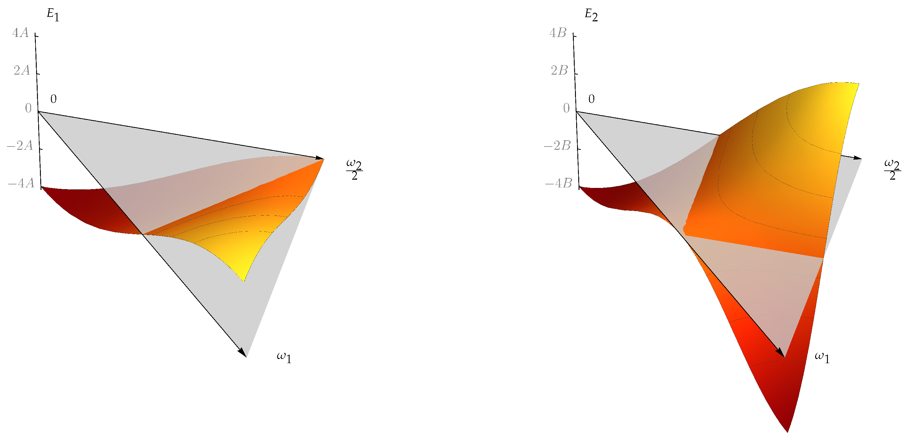
The energy functions $E_1,E_2:F^{\vee }\to \mathbb{R}$, which characterise the total eigenenergies of the quantum particle, are given for $b\in F^{\vee }$ by the following relations,

$$\begin{array}{cc}\hfill E_1\left(b\right)& =-A{C}_{{\omega }_2^{\vee }}\left(b\right),\hfill \end{array}$$

(76)

$$\begin{array}{cc}\hfill E_2\left(b\right)& =-B{C}_{{\omega }_1^{\vee }}\left(b\right).\hfill \end{array}$$

(77)

The 3D plots of energy functions $E_1$ and $E_2$ for the $C_2$ case are depicted in Figure 1.

The total eigenenergies of the quantum particle propagating on the dots $D_{P^{\vee },l,M}^{\sigma }(\varrho ,{\varrho }^{\vee })$ are determined for $\lambda \in {\Lambda }_{Q,M}^{\sigma }(\varrho ,{\varrho }^{\vee })$ from relation (59) by the energy functions as follows,

$$\begin{array}{c}\hfill E_{P^{\vee },\lambda ,M}^{\sigma }\left(\varrho ,{\varrho }^{\vee }\right)=E_0+E_1\left(\frac{\lambda }{M}\right)+E_2\left(\frac{\lambda }{M}\right).\end{array}$$

(78)

Dots $D_{P^{\vee },l,M}^{\sigma }\left(0,\frac{1}{2}{\omega }_1^{\vee }\right)$

For the fixed scaling factor $M=5$, the trivial admissible shift of the weight lattice $\varrho =0$ and the admissible shift of the dual weight lattice ${\varrho }^{\vee }={\omega }_1^{\vee }/2$, the point sets are determined in ${\omega }^{\vee }$-basis as follows:

$$\begin{array}{cc}\hfill F_{P^{\vee },5}^{\mathfrak{1}}\left(0,\frac{1}{2}{\omega }_1^{\vee }\right)& =\left\{\left(\frac{1}{10},\frac{4}{5}\right),\left(\frac{3}{10},\frac{2}{5}\right),\left(\frac{1}{2},0\right),\left(\frac{1}{10},\frac{3}{5}\right),\left(\frac{3}{10},\frac{1}{5}\right),\left(\frac{1}{10},\frac{2}{5}\right),\right.\hfill \\ \hfill & \phantom{=\{}\left.\left(\frac{3}{10},0\right),\left(\frac{1}{10},\frac{1}{5}\right),\left(\frac{1}{10},0\right)\right\},\hfill \end{array}$$

(79)

$$\begin{array}{cc}\hfill F_{P^{\vee },5}^{{\sigma }^e}\left(0,\frac{1}{2}{\omega }_1^{\vee }\right)& =\left\{\left(\frac{1}{10},\frac{3}{5}\right),\left(\frac{3}{10},\frac{1}{5}\right),\left(\frac{1}{10},\frac{2}{5}\right),\left(\frac{1}{10},\frac{1}{5}\right)\right\},\hfill \end{array}$$

(80)

$$\begin{array}{cc}\hfill F_{P^{\vee },5}^{{\sigma }^s}\left(0,\frac{1}{2}{\omega }_1^{\vee }\right)& =\left\{\left(\frac{1}{10},\frac{4}{5}\right),\left(\frac{3}{10},\frac{2}{5}\right),\left(\frac{1}{2},0\right),\left(\frac{1}{10},\frac{3}{5}\right),\left(\frac{3}{10},\frac{1}{5}\right),\left(\frac{1}{10},\frac{2}{5}\right),\right.\hfill \\ \hfill & \phantom{=\{}\left.\left(\frac{3}{10},0\right),\left(\frac{1}{10},\frac{1}{5}\right),\left(\frac{1}{10},0\right)\right\},\hfill \end{array}$$

(81)

$$\begin{array}{cc}\hfill F_{P^{\vee },5}^{{\sigma }^l}\left(0,\frac{1}{2}{\omega }_1^{\vee }\right)& =\left\{\left(\frac{1}{10},\frac{3}{5}\right),\left(\frac{3}{10},\frac{1}{5}\right),\left(\frac{1}{10},\frac{2}{5}\right),\left(\frac{1}{10},\frac{1}{5}\right)\right\}\hfill \end{array}$$

(82)

and the corresponding label sets are given in $\omega$-basis by the relations

$$\begin{array}{cc}\hfill {\Lambda }_{Q,5}^{\mathfrak{1}}\left(0,\frac{1}{2}{\omega }_1^{\vee }\right)=& \left\{\right(0,2),(2,1),(4,0),(1,1),(3,0),(0,1),(2,0),(1,0),(0,0\left)\right\},\hfill \end{array}$$

(83)

$$\begin{array}{cc}\hfill {\Lambda }_{Q,5}^{{\sigma }^e}\left(0,\frac{1}{2}{\omega }_1^{\vee }\right)=& \left\{\right(1,2),(3,1),(2,1),(1,1\left)\right\},\hfill \end{array}$$

(84)

$$\begin{array}{cc}\hfill {\Lambda }_{Q,5}^{{\sigma }^s}\left(0,\frac{1}{2}{\omega }_1^{\vee }\right)=& \left\{\right(1,2),(3,1),(5,0),(2,1),(4,0),(1,1),(3,0),(2,0),(1,0\left)\right\},\hfill \end{array}$$

(85)

$$\begin{array}{cc}\hfill {\Lambda }_{Q,5}^{{\sigma }^l}\left(0,\frac{1}{2}{\omega }_1^{\vee }\right)=& \left\{\right(0,2),(2,1),(1,1),(0,1\left)\right\}.\hfill \end{array}$$

(86)

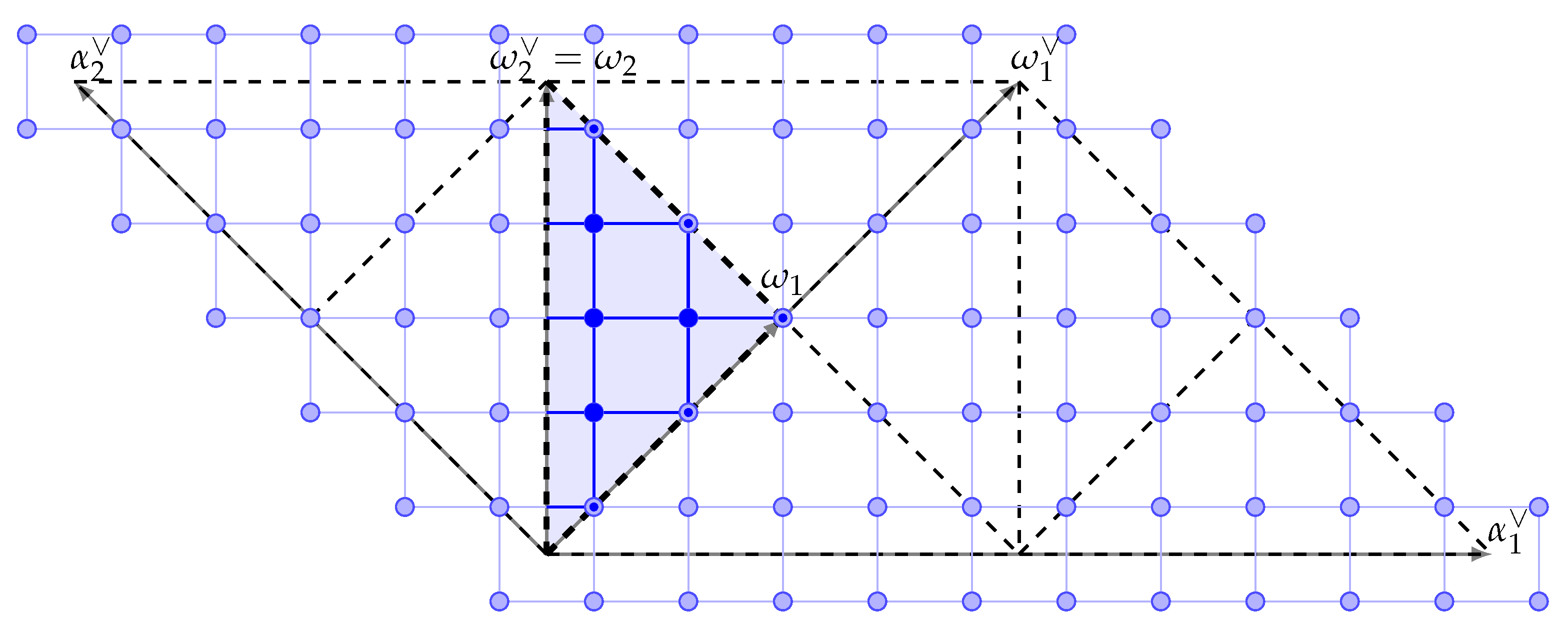
The determinant ${\sigma }^e$ sign homomorphism dot $D_{P^{\vee },1,5}^{{\sigma }^e}\left(0,\frac{1}{2}{\omega }_1^{\vee }\right)$ is depicted in Figure 2.

The matrices of the two dual-weight hopping operators (52) for the identity sign homomorphism, which is calculated in the position basis |a〉 ordered as points from list (79), are of the following form:

$${\widehat{A}}_{{\omega }_2^{\vee },5}^{\mathfrak{1}}\left(0,\frac{1}{2}{\omega }_1^{\vee }\right)=-A\left(\begin{array}{ccccccccc}2& 0& 0& \sqrt{2}& 0& 0& 0& 0& 0\\ 0& 0& 0& \sqrt{2}& \sqrt{2}& 0& 0& 0& 0\\ 0& 0& 0& 0& 2& 0& 0& 0& 0\\ \sqrt{2}& \sqrt{2}& 0& 1& 0& 1& 0& 0& 0\\ 0& \sqrt{2}& 2& 0& 0& 1& \sqrt{2}& 0& 0\\ 0& 0& 0& 1& 1& 1& 0& 1& 0\\ 0& 0& 0& 0& \sqrt{2}& 0& 0& \sqrt{2}& 0\\ 0& 0& 0& 0& 0& 1& \sqrt{2}& 1& \sqrt{2}\\ 0& 0& 0& 0& 0& 0& 0& \sqrt{2}& 2\end{array}\right)$$

and

$${\widehat{A}}_{{\omega }_1^{\vee },5}^{\mathfrak{1}}\left(0,\frac{1}{2}{\omega }_1^{\vee }\right)=-B\left(\begin{array}{ccccccccc}1& 1& 0& \sqrt{2}& 0& 0& 0& 0& 0\\ 1& 0& \sqrt{2}& 0& 0& \sqrt{2}& 0& 0& 0\\ 0& \sqrt{2}& 0& 0& 0& 0& \sqrt{2}& 0& 0\\ \sqrt{2}& 0& 0& 1& 1& 1& 0& 0& 0\\ 0& 0& 0& 1& 2& 0& 0& 1& 0\\ 0& \sqrt{2}& 0& 1& 0& 0& \sqrt{2}& 1& 0\\ 0& 0& \sqrt{2}& 0& 0& \sqrt{2}& 0& 0& 1\\ 0& 0& 0& 0& 1& 1& 0& 1& \sqrt{2}\\ 0& 0& 0& 0& 0& 0& 1& \sqrt{2}& 1\end{array}\right).$$

Calculated in the position basis |a〉 ordered as points from list (80), the matrices of the two dual-weight hopping operators for the determinant sign homomorphism ${\sigma }^e$ are determined as follows:

$${\widehat{A}}_{{\omega }_2^{\vee },5}^{{\sigma }^e}\left(0,\frac{1}{2}{\omega }_1^{\vee }\right)=-A\left(\begin{array}{cccc}-1& 0& 1& 0\\ 0& 0& 1& 0\\ 1& 1& -1& 1\\ 0& 0& 1& -1\end{array}\right)$$

and

$${\widehat{A}}_{{\omega }_1^{\vee },5}^{{\sigma }^e}\left(0,\frac{1}{2}{\omega }_1^{\vee }\right)=-B\left(\begin{array}{cccc}-1& 1& -1& 0\\ 1& -2& 0& 1\\ -1& 0& 0& -1\\ 0& 1& -1& -1\end{array}\right).$$

Calculated in the position basis |a〉 ordered as points from list (81), the matrices of the two dual-weight hopping operators for the short sign homomorphism ${\sigma }^s$ are given as follows:

$${\widehat{A}}_{{\omega }_2^{\vee },5}^{{\sigma }^s}\left(0,\frac{1}{2}{\omega }_1^{\vee }\right)=-A\left(\begin{array}{ccccccccc}-2& 0& 0& \sqrt{2}& 0& 0& 0& 0& 0\\ 0& 0& 0& \sqrt{2}& \sqrt{2}& 0& 0& 0& 0\\ 0& 0& 0& 0& 2& 0& 0& 0& 0\\ \sqrt{2}& \sqrt{2}& 0& -1& 0& 1& 0& 0& 0\\ 0& \sqrt{2}& 2& 0& 0& 1& \sqrt{2}& 0& 0\\ 0& 0& 0& 1& 1& -1& 0& 1& 0\\ 0& 0& 0& 0& \sqrt{2}& 0& 0& \sqrt{2}& 0\\ 0& 0& 0& 0& 0& 1& \sqrt{2}& -1& \sqrt{2}\\ 0& 0& 0& 0& 0& 0& 0& \sqrt{2}& -2\end{array}\right)$$

and

$${\widehat{A}}_{{\omega }_1^{\vee },5}^{{\sigma }^s}\left(0,\frac{1}{2}{\omega }_1^{\vee }\right)=-B\left(\begin{array}{ccccccccc}1& 1& 0& -\sqrt{2}& 0& 0& 0& 0& 0\\ 1& 0& \sqrt{2}& 0& 0& \sqrt{2}& 0& 0& 0\\ 0& \sqrt{2}& 0& 0& 0& 0& \sqrt{2}& 0& 0\\ -\sqrt{2}& 0& 0& 1& 1& -1& 0& 0& 0\\ 0& 0& 0& 1& 2& 0& 0& 1& 0\\ 0& \sqrt{2}& 0& -1& 0& 0& \sqrt{2}& -1& 0\\ 0& 0& \sqrt{2}& 0& 0& \sqrt{2}& 0& 0& 1\\ 0& 0& 0& 0& 1& -1& 0& 1& -\sqrt{2}\\ 0& 0& 0& 0& 0& 0& 1& -\sqrt{2}& 1\end{array}\right).$$

The matrices of the two dual-weight hopping operators for the long sign homomorphism ${\sigma }^l$, which are calculated in the position basis |a〉 ordered as points from list (82), are of the following form:

$${\widehat{A}}_{{\omega }_2^{\vee },5}^{{\sigma }^l}\left(0,\frac{1}{2}{\omega }_1^{\vee }\right)=-A\left(\begin{array}{cccc}1& 0& 1& 0\\ 0& 0& 1& 0\\ 1& 1& 1& 1\\ 0& 0& 1& 1\end{array}\right)$$

and

$${\widehat{A}}_{{\omega }_1^{\vee },5}^{{\sigma }^l}\left(0,\frac{1}{2}{\omega }_1^{\vee }\right)=-B\left(\begin{array}{cccc}-1& 1& 1& 0\\ 1& -2& 0& 1\\ 1& 0& 0& 1\\ 0& 1& 1& -1\end{array}\right).$$

The four Hamiltonians of the quantum particle on the dual-weight dots $D_{P^{\vee },l,5}^{\sigma }\left(0,\frac{1}{2}{\omega }_1^{\vee }\right)$ are then given as follows,

$$\begin{array}{c}\hfill {\widehat{H}}_{P^{\vee },5}^{\mathfrak{1}}\left(0,\frac{1}{2}{\omega }_1^{\vee }\right)={\widehat{A}}_{0,5}^{\mathfrak{1}}\left(0,\frac{1}{2}{\omega }_1^{\vee }\right)+{\widehat{A}}_{{\omega }_2^{\vee },5}^{\mathfrak{1}}\left(0,\frac{1}{2}{\omega }_1^{\vee }\right)+{\widehat{A}}_{{\omega }_1^{\vee },5}^{\mathfrak{1}}\left(0,\frac{1}{2}{\omega }_1^{\vee }\right),\\ \hfill {\widehat{H}}_{P^{\vee },5}^{{\sigma }^e}\left(0,\frac{1}{2}{\omega }_1^{\vee }\right)={\widehat{A}}_{0,5}^{{\sigma }^e}\left(0,\frac{1}{2}{\omega }_1^{\vee }\right)+{\widehat{A}}_{{\omega }_2^{\vee },5}^{{\sigma }^e}\left(0,\frac{1}{2}{\omega }_1^{\vee }\right)+{\widehat{A}}_{{\omega }_1^{\vee },5}^{{\sigma }^e}\left(0,\frac{1}{2}{\omega }_1^{\vee }\right),\\ \hfill {\widehat{H}}_{P^{\vee },5}^{{\sigma }^s}\left(0,\frac{1}{2}{\omega }_1^{\vee }\right)={\widehat{A}}_{0,5}^{{\sigma }^s}\left(0,\frac{1}{2}{\omega }_1^{\vee }\right)+{\widehat{A}}_{{\omega }_2^{\vee },5}^{{\sigma }^s}\left(0,\frac{1}{2}{\omega }_1^{\vee }\right)+{\widehat{A}}_{{\omega }_1^{\vee },5}^{{\sigma }^s}\left(0,\frac{1}{2}{\omega }_1^{\vee }\right),\\ \hfill {\widehat{H}}_{P^{\vee },5}^{{\sigma }^l}\left(0,\frac{1}{2}{\omega }_1^{\vee }\right)={\widehat{A}}_{0,5}^{{\sigma }^l}\left(0,\frac{1}{2}{\omega }_1^{\vee }\right)+{\widehat{A}}_{{\omega }_2^{\vee },5}^{{\sigma }^l}\left(0,\frac{1}{2}{\omega }_1^{\vee }\right)+{\widehat{A}}_{{\omega }_1^{\vee },5}^{{\sigma }^l}\left(0,\frac{1}{2}{\omega }_1^{\vee }\right).\end{array}$$

The set of (rounded) eigenenergies of the particle on the identity homomorphism dot $D_{Q^{\vee },l,5}^{\mathfrak{1}}\left(0,\frac{1}{2}{\omega }_1^{\vee }\right)$ is calculated from relation (78) in the ordering of the label set (83) as follows:

$$\begin{array}{cc}\hfill \left\{E_{P^{\vee },\lambda ,5}^{\mathfrak{1}}\left(0,\frac{1}{2}{\omega }_1^{\vee }\right)\mid \lambda \right.& \left.\in {\Lambda }_{Q,5}^{\mathfrak{1}}\left(0,\frac{1}{2}{\omega }_1^{\vee }\right)\right\}=E_0\left\{1,1,1,1,1,1,1,1,1\right\}\hfill \\ \hfill & +A\left\{-0.382,1,3.236,-1,1.236,-2.618,-1.236,-3.236,-4\right\}\hfill \\ \hfill & +B\left\{3.236,1,-2.618,1,-0.382,-1.236,-0.382,-2.618,-4\right\}\hfill \end{array}$$

and on the determinant sign homomorphism dot $D_{Q^{\vee },l,5}^{{\sigma }^e}\left(0,\frac{1}{2}{\omega }_1^{\vee }\right)$ in the ordering of the label set (84) as follows:

$$\begin{array}{cc}\hfill \left\{E_{P^{\vee },\lambda ,5}^{{\sigma }^e}\left(0,\frac{1}{2}{\omega }_1^{\vee }\right)\mid \lambda \in {\Lambda }_{Q,5}^{{\sigma }^e}\left(0,\frac{1}{2}{\omega }_1^{\vee }\right)\right\}=& E_0\left\{1,1,1,1\right\}\hfill \\ \hfill & +A\left\{0.382,2.618,1,-1\right\}\hfill \\ \hfill & +B\left\{3.236,-1.236,1,1\right\}.\hfill \end{array}$$

For the short homomorphism dot $D_{Q^{\vee },l,5}^{{\sigma }^s}\left(0,\frac{1}{2}{\omega }_1^{\vee }\right)$, the set of rounded eigenenergies of the quantum particle in the ordering of the label set (85) is calculated as follows:

$$\begin{array}{cc}\hfill \left\{E_{P^{\vee },\lambda ,5}^{{\sigma }^s}\left(0,\frac{1}{2}{\omega }_1^{\vee }\right)\mid \lambda \right.& \left.\in {\Lambda }_{Q,5}^{{\sigma }^s}\left(0,\frac{1}{2}{\omega }_1^{\vee }\right)\right\}=E_0\left\{1,1,1,1,1,1,1,1,1\right\}\hfill \\ \hfill & +A\left\{0.382,2.618,4,1,3.236,-1,1.236,-1.236,-3.236\right\}\hfill \\ \hfill & +B\left\{3.236,-1.236,-4,1,-2.618,1,-0.382,-0.382,-2.618\right\}\hfill \end{array}$$

and for the long homomorphism dot $D_{Q^{\vee },l,5}^{{\sigma }^l}\left(0,\frac{1}{2}{\omega }_1^{\vee }\right)$ in the ordering of the label set (86) as the following:

$$\begin{array}{cc}\hfill \left\{E_{P^{\vee },\lambda ,5}^{{\sigma }^l}\left(0,\frac{1}{2}{\omega }_1^{\vee }\right)\mid \lambda \in {\Lambda }_{Q,5}^{{\sigma }^l}\left(0,\frac{1}{2}{\omega }_1^{\vee }\right)\right\}=& E_0\left\{1,1,1,1\right\}\hfill \\ \hfill & +A\left\{-0.382,1,-1,-2.618\right\}\hfill \\ \hfill & +B\left\{3.236,1,1,-1.236\right\}.\hfill \end{array}$$

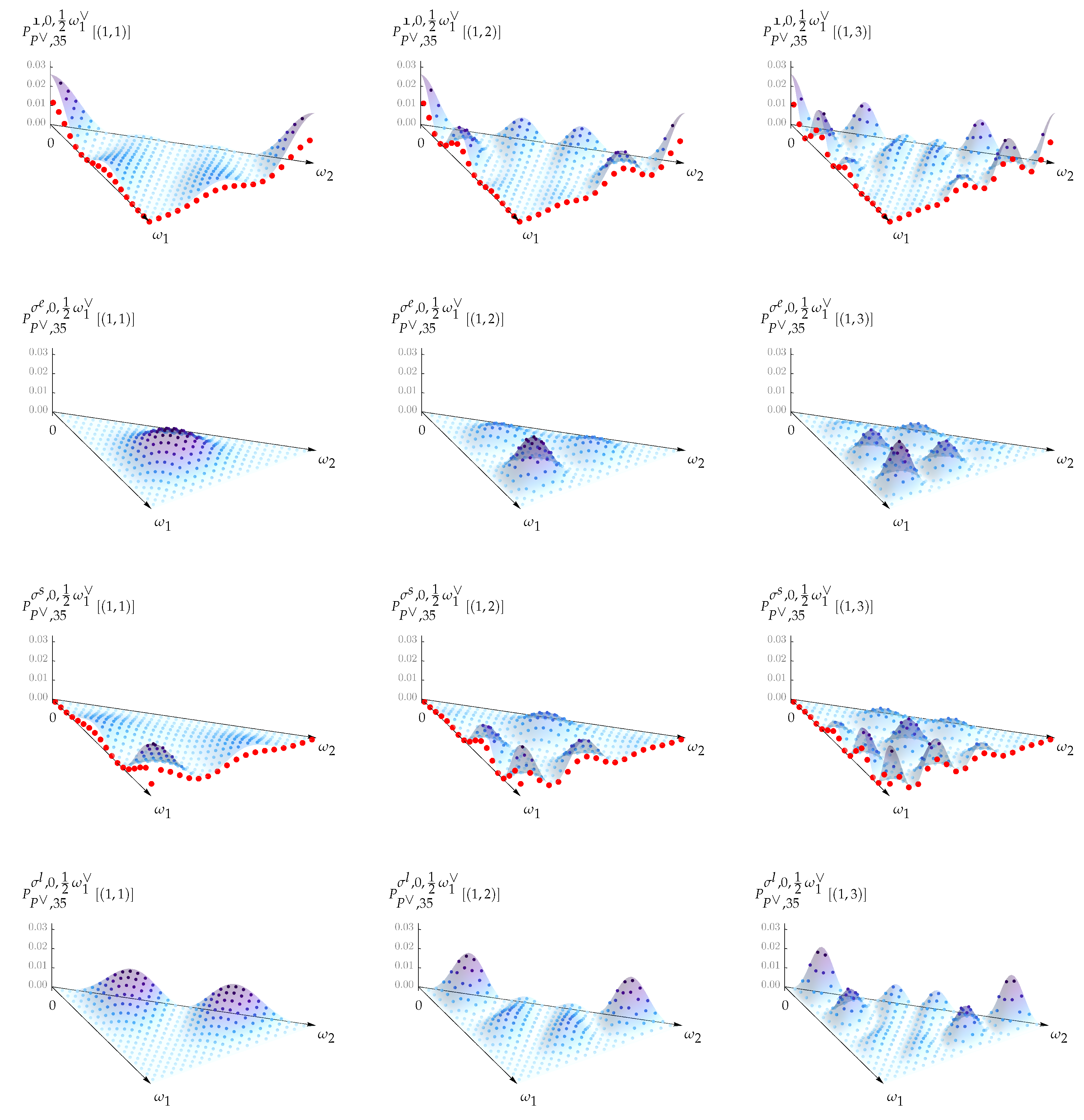
The probabilities $P_{P^{\vee },35}^{\sigma ,0,\frac{1}{2}{\omega }_1^{\vee }}\left[\lambda \right]$ of finding the particle on the dots $D_{P^{\vee },1,35}^{\sigma }\left(0,\frac{1}{2}{\omega }_1^{\vee }\right)$, $\sigma \in \{\mathfrak{1},{\sigma }^e,{\sigma }^s,{\sigma }^l\}$ corresponding to several lower stationary states $|\lambda \rangle$ are depicted in Figure 3.

4.2. Case $G_2$

The root system $G_2$ admits only the trivial shifts for both weight and dual weight lattices [18]. Considering only the nearest and next-to-nearest neighbour coupling, the three non-zero values of the dual-weight hopping function ${\mathcal{P}}^{\vee }$ are determined by the zero energy level $E_0$ and two non-zero parameters $A,B\in \mathbb{R}$ as follows,

$$\begin{array}{cc}\hfill {\mathcal{P}}^{\vee }\left(0\right)& =-E_0,\hfill \\ \hfill {\mathcal{P}}^{\vee }\left({\omega }_1^{\vee }\right)& =A,\hfill \\ \hfill {\mathcal{P}}^{\vee }\left({\omega }_2^{\vee }\right)& =B.\hfill \end{array}$$

(87)

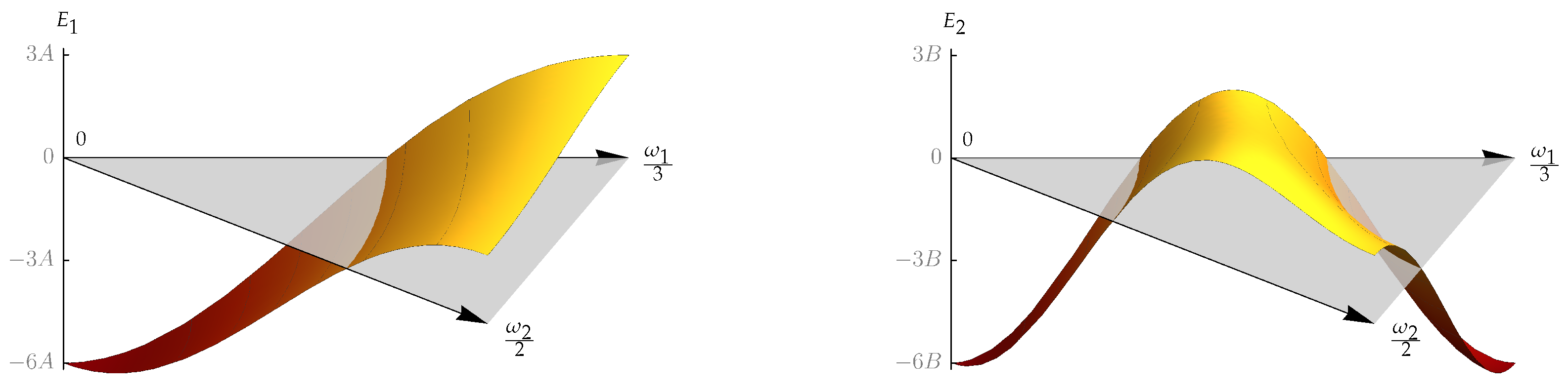
The energy functions $E_1,E_2:F^{\vee }\to \mathbb{R}$ that characterise the total eigenenergies of the quantum particle are specified for $b\in F^{\vee }$ by the following relations,

$$\begin{array}{cc}\hfill E_1\left(b\right)& =-A{C}_{{\omega }_1^{\vee }}\left(b\right),\hfill \end{array}$$

(88)

$$\begin{array}{cc}\hfill E_2\left(b\right)& =-B{C}_{{\omega }_2^{\vee }}\left(b\right).\hfill \end{array}$$

(89)

The 3D plots of the energy functions $E_1$ and $E_2$ are depicted in Figure 4.

Stemming from relation (59), the total eigenenergies are for $\lambda \in {\Lambda }_{Q,M}^{\sigma }(0,0)$ determined by the energy functions $E_1$ and $E_2$ as the following,

$$\begin{array}{c}\hfill E_{P^{\vee },\lambda ,M}^{\sigma }(0,0)=E_0+E_1\left(\frac{\lambda }{M}\right)+E_2\left(\frac{\lambda }{M}\right).\end{array}$$

(90)

Dots $D_{P^{\vee },l,M}^{\sigma }(0,0)$

The four point sets (37) are for the fixed scaling factor $M=10$ expressed in ${\omega }^{\vee }$-basis as the following:

$$\begin{array}{cc}\hfill F_{P^{\vee },10}^{\mathfrak{1}}(0,0)& =\left\{\left(\frac{1}{5},\frac{1}{5}\right),\left(\frac{1}{2},0\right),\left(0,\frac{3}{10}\right),\left(\frac{3}{10},\frac{1}{10}\right),\left(\frac{1}{10},\frac{1}{5}\right),\left(\frac{2}{5},0\right),\left(\frac{1}{5},\frac{1}{10}\right),\left(0,\frac{1}{5}\right),\right.\hfill \\ \hfill & \phantom{=\{}\left.\left(\frac{3}{10},0\right),\left(\frac{1}{10},\frac{1}{10}\right),\left(\frac{1}{5},0\right),\left(0,\frac{1}{10}\right),\left(\frac{1}{10},0\right),\left(0,0\right)\right\},\hfill \end{array}$$

(91)

$$\begin{array}{cc}\hfill F_{P^{\vee },10}^{{\sigma }^e}(0,0)& =\left\{\left(\frac{3}{10},\frac{1}{10}\right),\left(\frac{1}{10},\frac{1}{5}\right),\left(\frac{1}{5},\frac{1}{10}\right),\left(\frac{1}{10},\frac{1}{10}\right)\right\},\hfill \end{array}$$

(92)

$$\begin{array}{cc}\hfill F_{P^{\vee },10}^{{\sigma }^s}(0,0)& =\left\{\left(\frac{1}{5},\frac{1}{5}\right),\left(0,\frac{3}{10}\right),\left(\frac{3}{10},\frac{1}{10}\right),\left(\frac{1}{10},\frac{1}{5}\right),\left(\frac{1}{5},\frac{1}{10}\right),\left(0,\frac{1}{5}\right),\left(\frac{1}{10},\frac{1}{10}\right),\left(0,\frac{1}{10}\right)\right\},\hfill \end{array}$$

(93)

$$\begin{array}{cc}\hfill F_{P^{\vee },10}^{{\sigma }^l}(0,0)& =\left\{\left(\frac{3}{10},\frac{1}{10}\right),\left(\frac{1}{10},\frac{1}{5}\right),\left(\frac{2}{5},0\right),\left(\frac{1}{5},\frac{1}{10}\right),\left(\frac{3}{10},0\right),\left(\frac{1}{10},\frac{1}{10}\right),\left(\frac{1}{5},0\right),\left(\frac{1}{10},0\right)\right\}\hfill \end{array}$$

(94)

and the label sets (38) are determined in $\omega$-basis as the following:

$$\begin{array}{cc}\hfill {\Lambda }_{Q,10}^{\mathfrak{1}}(0,0)=& \left\{\right(0,5),(2,2),(1,3),(3,0),(0,4),(2,1),(1,2),(0,3),(2,0),(1,1),\hfill \\ \hfill & \phantom{\}}(0,2),(1,0),(0,1),(0,0)\},\hfill \end{array}$$

(95)

$$\begin{array}{cc}\hfill {\Lambda }_{Q,10}^{{\sigma }^e}(0,0)=& \left\{\right(1,3),(2,1),(1,2),(1,1\left)\right\},\hfill \end{array}$$

(96)

$$\begin{array}{cc}\hfill {\Lambda }_{Q,10}^{{\sigma }^s}(0,0)=& \left\{\right(1,3),(0,4),(2,1),(1,2),(0,3),(1,1),(0,2),(0,1\left)\right\},\hfill \end{array}$$

(97)

$$\begin{array}{cc}\hfill {\Lambda }_{Q,10}^{{\sigma }^l}(0,0)=& \left\{\right(2,2),(1,3),(3,0),(2,1),(1,2),(2,0),(1,1),(1,0\left)\right\}.\hfill \end{array}$$

(98)

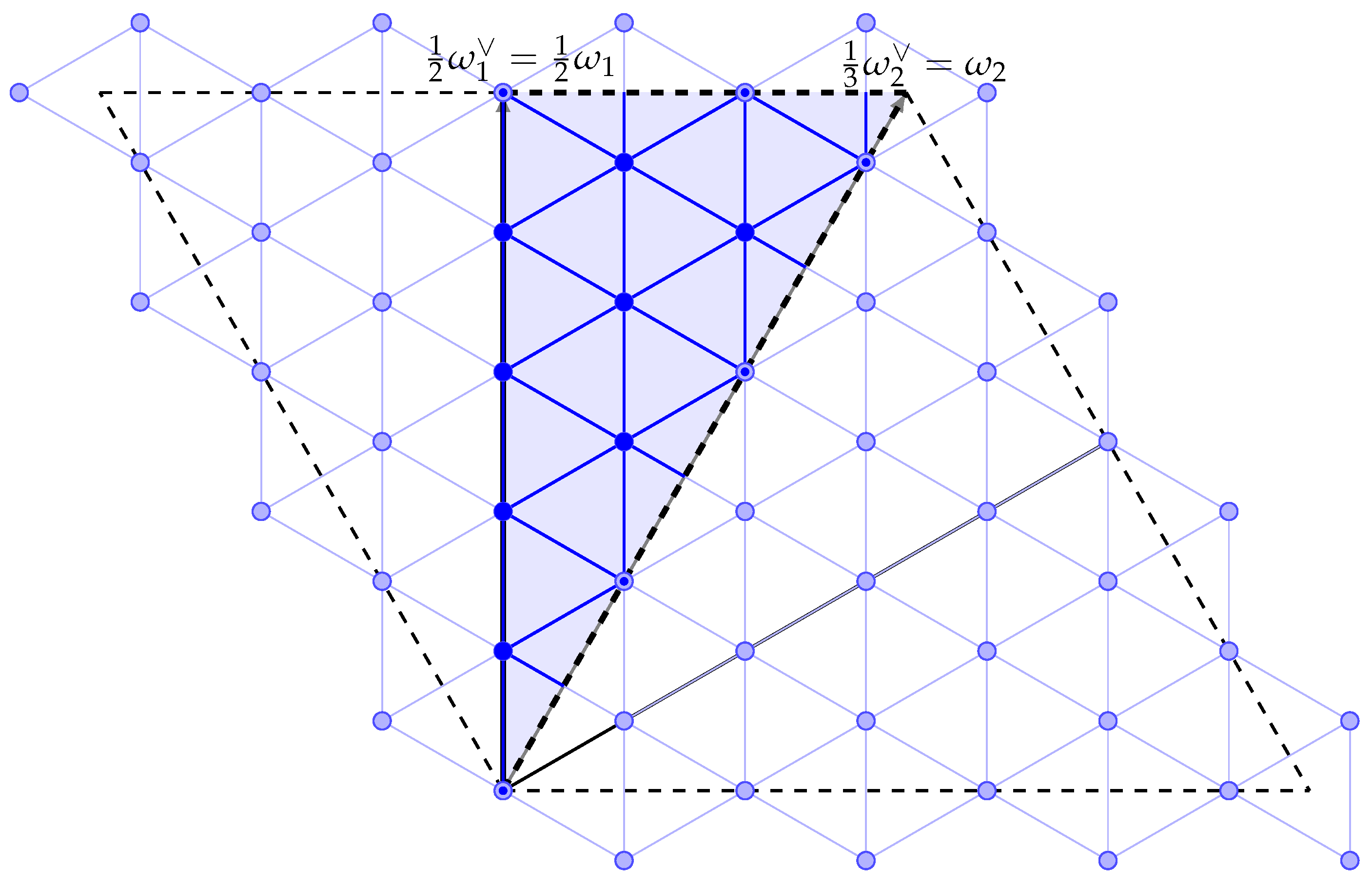
The long sign homomorphism dual-weight dot $D_{P^{\vee },1,10}^{{\sigma }^l}(0,0)$ is depicted in Figure 5.

Calculated in the position basis |a〉 that is ordered as the points listed in expression (91), the two identity sign homomorphism dual-weight hopping operators (52) are determined as follows:

$${\widehat{A}}_{{\omega }_1^{\vee },10}^{\mathfrak{1}}(0,0)=-A\left(\begin{array}{cccccccccccccc}0& 0& 2& \sqrt{2}& \sqrt{2}& 0& 0& 0& 0& 0& 0& 0& 0& 0\\ 0& 0& 0& 2& 0& \sqrt{2}& 0& 0& 0& 0& 0& 0& 0& 0\\ 2& 0& 2& 0& \sqrt{2}& 0& 0& 0& 0& 0& 0& 0& 0& 0\\ \sqrt{2}& 2& 0& 1& 1& \sqrt{2}& 1& 0& 0& 0& 0& 0& 0& 0\\ \sqrt{2}& 0& \sqrt{2}& 1& 1& 0& 1& \sqrt{2}& 0& 0& 0& 0& 0& 0\\ 0& \sqrt{2}& 0& \sqrt{2}& 0& 0& \sqrt{2}& 0& 1& 0& 0& 0& 0& 0\\ 0& 0& 0& 1& 1& \sqrt{2}& 0& \sqrt{2}& \sqrt{2}& 1& 0& 0& 0& 0\\ 0& 0& 0& 0& \sqrt{2}& 0& \sqrt{2}& 0& 0& \sqrt{2}& 0& 0& 0& 0\\ 0& 0& 0& 0& 0& 1& \sqrt{2}& 0& 0& \sqrt{2}& 1& 0& 0& 0\\ 0& 0& 0& 0& 0& 0& 1& \sqrt{2}& \sqrt{2}& 1& \sqrt{2}& \sqrt{2}& 0& 0\\ 0& 0& 0& 0& 0& 0& 0& 0& 1& \sqrt{2}& 0& 2& 1& 0\\ 0& 0& 0& 0& 0& 0& 0& 0& 0& \sqrt{2}& 2& 0& 2& 0\\ 0& 0& 0& 0& 0& 0& 0& 0& 0& 0& 1& 2& 2& \sqrt{6}\\ 0& 0& 0& 0& 0& 0& 0& 0& 0& 0& 0& 0& \sqrt{6}& 0\end{array}\right)$$

and

$${\widehat{A}}_{{\omega }_2^{\vee },10}^{\mathfrak{1}}(0,0)=-B\left(\begin{array}{cccccccccccccc}0& \sqrt{2}& 1& 0& \sqrt{2}& 0& \sqrt{2}& 0& 0& 0& 0& 0& 0& 0\\ \sqrt{2}& 0& 0& 0& 0& 0& 2& 0& 0& 0& 0& 0& 0& 0\\ 1& 0& 0& \sqrt{2}& \sqrt{2}& 0& 0& 1& 0& 0& 0& 0& 0& 0\\ 0& 0& \sqrt{2}& 1& 1& \sqrt{2}& 0& \sqrt{2}& \sqrt{2}& 0& 0& 0& 0& 0\\ \sqrt{2}& 0& \sqrt{2}& 1& 0& \sqrt{2}& 1& 0& 0& 1& 0& 0& 0& 0\\ 0& 0& 0& \sqrt{2}& \sqrt{2}& 0& 0& 0& 0& \sqrt{2}& 0& 0& 0& 0\\ \sqrt{2}& 2& 0& 0& 1& 0& 1& 0& 0& 1& \sqrt{2}& 0& 0& 0\\ 0& 0& 1& \sqrt{2}& 0& 0& 0& 0& 2& 0& 0& 1& 0& 0\\ 0& 0& 0& \sqrt{2}& 0& 0& 0& 2& 0& 0& 0& 2& 0& 0\\ 0& 0& 0& 0& 1& \sqrt{2}& 1& 0& 0& 1& \sqrt{2}& 0& \sqrt{2}& 0\\ 0& 0& 0& 0& 0& 0& \sqrt{2}& 0& 0& \sqrt{2}& 0& 0& 2& 0\\ 0& 0& 0& 0& 0& 0& 0& 1& 2& 0& 0& 2& 0& \sqrt{6}\\ 0& 0& 0& 0& 0& 0& 0& 0& 0& \sqrt{2}& 2& 0& 2& 0\\ 0& 0& 0& 0& 0& 0& 0& 0& 0& 0& 0& \sqrt{6}& 0& 0\end{array}\right).$$

Calculated in the position basis |a〉 that is ordered as the points listed in expression (92), the two determinant sign homomorphism dual-weight hopping operators are given as the following:

$${\widehat{A}}_{{\omega }_1^{\vee },10}^{{\sigma }^e}(0,0)=-A\left(\begin{array}{cccc}-1& 1& 1& 0\\ 1& -1& 1& 0\\ 1& 1& 0& 1\\ 0& 0& 1& -1\end{array}\right)$$

and

$${\widehat{A}}_{{\omega }_2^{\vee },10}^{{\sigma }^e}(0,0)=-B\left(\begin{array}{cccc}-1& -1& 0& 0\\ -1& 0& -1& 1\\ 0& -1& -1& -1\\ 0& 1& -1& -1\end{array}\right).$$

The two short sign homomorphism dual-weight hopping operators, which are calculated in the position basis |a〉 ordered as the points from the list (93), are given as the following:

$${\widehat{A}}_{{\omega }_1^{\vee },10}^{{\sigma }^s}(0,0)=-A\left(\begin{array}{cccccccc}0& 2& \sqrt{2}& \sqrt{2}& 0& 0& 0& 0\\ 2& 2& 0& \sqrt{2}& 0& 0& 0& 0\\ \sqrt{2}& 0& 1& 1& 1& 0& 0& 0\\ \sqrt{2}& \sqrt{2}& 1& 1& 1& \sqrt{2}& 0& 0\\ 0& 0& 1& 1& 0& \sqrt{2}& 1& 0\\ 0& 0& 0& \sqrt{2}& \sqrt{2}& 0& \sqrt{2}& 0\\ 0& 0& 0& 0& 1& \sqrt{2}& 1& \sqrt{2}\\ 0& 0& 0& 0& 0& 0& \sqrt{2}& 0\end{array}\right)$$

and

$${\widehat{A}}_{{\omega }_2^{\vee },10}^{{\sigma }^s}(0,0)=-B\left(\begin{array}{cccccccc}0& 1& 0& \sqrt{2}& \sqrt{2}& 0& 0& 0\\ 1& 0& \sqrt{2}& \sqrt{2}& 0& 1& 0& 0\\ 0& \sqrt{2}& -1& 1& 0& \sqrt{2}& 0& 0\\ \sqrt{2}& \sqrt{2}& 1& 0& 1& 0& 1& 0\\ \sqrt{2}& 0& 0& 1& -1& 0& 1& 0\\ 0& 1& \sqrt{2}& 0& 0& 0& 0& 1\\ 0& 0& 0& 1& 1& 0& -1& 0\\ 0& 0& 0& 0& 0& 1& 0& -2\end{array}\right).$$

The two long sign homomorphism dual-weight hopping operators, which are calculated in the position basis |a〉 ordered as the points from the list (94), are given as the following:

$${\widehat{A}}_{{\omega }_1^{\vee },10}^{{\sigma }^l}(0,0)=-A\left(\begin{array}{cccccccc}-1& 1& \sqrt{2}& 1& 0& 0& 0& 0\\ 1& -1& 0& 1& 0& 0& 0& 0\\ \sqrt{2}& 0& 0& \sqrt{2}& 1& 0& 0& 0\\ 1& 1& \sqrt{2}& 0& \sqrt{2}& 1& 0& 0\\ 0& 0& 1& \sqrt{2}& 0& \sqrt{2}& 1& 0\\ 0& 0& 0& 1& \sqrt{2}& -1& \sqrt{2}& 0\\ 0& 0& 0& 0& 1& \sqrt{2}& 0& 1\\ 0& 0& 0& 0& 0& 0& 1& -2\end{array}\right)$$

and

$${\widehat{A}}_{{\omega }_2^{\vee },10}^{{\sigma }^l}(0,0)=-B\left(\begin{array}{cccccccc}1& -1& -\sqrt{2}& 0& \sqrt{2}& 0& 0& 0\\ -1& 0& \sqrt{2}& -1& 0& 1& 0& 0\\ -\sqrt{2}& \sqrt{2}& 0& 0& 0& \sqrt{2}& 0& 0\\ 0& -1& 0& 1& 0& -1& \sqrt{2}& 0\\ \sqrt{2}& 0& 0& 0& 0& 0& 0& 0\\ 0& 1& \sqrt{2}& -1& 0& 1& -\sqrt{2}& \sqrt{2}\\ 0& 0& 0& \sqrt{2}& 0& -\sqrt{2}& 0& -2\\ 0& 0& 0& 0& 0& \sqrt{2}& -2& 2\end{array}\right).$$

The Hamiltonians of the quantum particle on the dual-weight dots $D_{P^{\vee },l,10}^{\mathfrak{1}}(0,0)$, $D_{P^{\vee },l,10}^{{\sigma }^e}(0,0)$, $D_{P^{\vee },l,10}^{{\sigma }^s}(0,0)$ and $D_{P^{\vee },l,10}^{{\sigma }^l}(0,0)$ are the sums (54) of the corresponding hopping operators,

$$\begin{array}{c}\hfill {\widehat{H}}_{P^{\vee },10}^{\mathfrak{1}}(0,0)={\widehat{A}}_{0,10}^{\mathfrak{1}}(0,0)+{\widehat{A}}_{{\omega }_1^{\vee },10}^{\mathfrak{1}}(0,0)+{\widehat{A}}_{{\omega }_2^{\vee },10}^{\mathfrak{1}}(0,0),\\ \hfill {\widehat{H}}_{P^{\vee },10}^{{\sigma }^e}(0,0)={\widehat{A}}_{0,10}^{{\sigma }^e}(0,0)+{\widehat{A}}_{{\omega }_1^{\vee },10}^{{\sigma }^e}(0,0)+{\widehat{A}}_{{\omega }_2^{\vee },10}^{{\sigma }^e}(0,0),\\ \hfill {\widehat{H}}_{P^{\vee },10}^{{\sigma }^s}(0,0)={\widehat{A}}_{0,10}^{{\sigma }^s}(0,0)+{\widehat{A}}_{{\omega }_1^{\vee },10}^{{\sigma }^s}(0,0)+{\widehat{A}}_{{\omega }_2^{\vee },10}^{{\sigma }^s}(0,0),\\ \hfill {\widehat{H}}_{P^{\vee },10}^{{\sigma }^l}(0,0)={\widehat{A}}_{0,10}^{{\sigma }^l}(0,0)+{\widehat{A}}_{{\omega }_1^{\vee },10}^{{\sigma }^l}(0,0)+{\widehat{A}}_{{\omega }_2^{\vee },10}^{{\sigma }^l}(0,0).\end{array}$$

The set of (rounded) eigenenergies of the particle on the identity sign homomorphism dot $D_{P^{\vee },l,10}^{\mathfrak{1}}(0,0)$ is computed from relation (90) in the ordering of the label set (95) as follows:

$$\begin{array}{cc}\hfill & \left\{E_{P^{\vee },\lambda ,10}^{\mathfrak{1}}(0,0)\mid \lambda \in {\Lambda }_{Q,10}^{\mathfrak{1}}(0,0)\right\}=E_0\left\{1,1,1,1,1,1,1,1,1,1,1,1,1,1\right\}\hfill \\ \hfill & +A\left\{2,2.618,2,2.854,1.236,2,0.618,-0.764,0.382,-1.618,-3.236,-3.854,-5.236,-6\right\}\hfill \\ \hfill & +B\left\{2,-3.236,0.618,-5.236,2.618,-1.618,2,2.854,1.236,2,0.382,-0.764,-3.854,-6\right\}\hfill \end{array}$$

and on the determinant sign homomorphism dot $D_{P^{\vee },l,10}^{{\sigma }^e}(0,0)$ in the ordering of the label set (96) as follows:

$$\begin{array}{cc}\hfill \left\{E_{P^{\vee },\lambda ,10}^{{\sigma }^e}(0,0)\mid \lambda \in {\Lambda }_{Q,10}^{{\sigma }^e}(0,0)\right\}=& E_0\left\{1,1,1,1\right\}\hfill \\ \hfill & +A\left\{2,2,0.618,-1.618\right\}\hfill \\ \hfill & +B\left\{0.618,-1.618,2,2\right\}.\hfill \end{array}$$

The set of eigenenergies of the particle on the short sign homomorphism dot $D_{P^{\vee },l,10}^{{\sigma }^s}(0,0)$ in the ordering of the label set (97) is provided by the following:

$$\begin{array}{cc}\hfill \left\{E_{P^{\vee },\lambda ,10}^{{\sigma }^s}(0,0)\mid \lambda \in {\Lambda }_{Q,10}^{{\sigma }^s}(0,0)\right\}=& E_0\left\{1,1,1,1,1,1,1,1\right\}\hfill \\ \hfill & +A\left\{2,1.236,2,0.618,-0.764,-1.618,-3.236,-5.236\right\}\hfill \\ \hfill & +B\left\{0.618,2.618,-1.618,2,2.854,2,0.382,-3.854\right\}\hfill \end{array}$$

and on the long sign homomorphism dot $D_{P^{\vee },l,10}^{{\sigma }^l}(0,0)$ in the ordering of the label set (98) by the following:

$$\begin{array}{cc}\hfill \left\{E_{P^{\vee },\lambda ,10}^{{\sigma }^l}(0,0)\mid \lambda \in {\Lambda }_{Q,10}^{{\sigma }^l}(0,0)\right\}=& E_0\left\{1,1,1,1,1,1,1,1\right\}\hfill \\ \hfill & +A\left\{2.618,2,2.854,2,0.618,0.382,-1.618,-3.854\right\}\hfill \\ \hfill & +B\left\{-3.236,0.618,-5.236,-1.618,2,1.236,2,-0.764\right\}.\hfill \end{array}$$

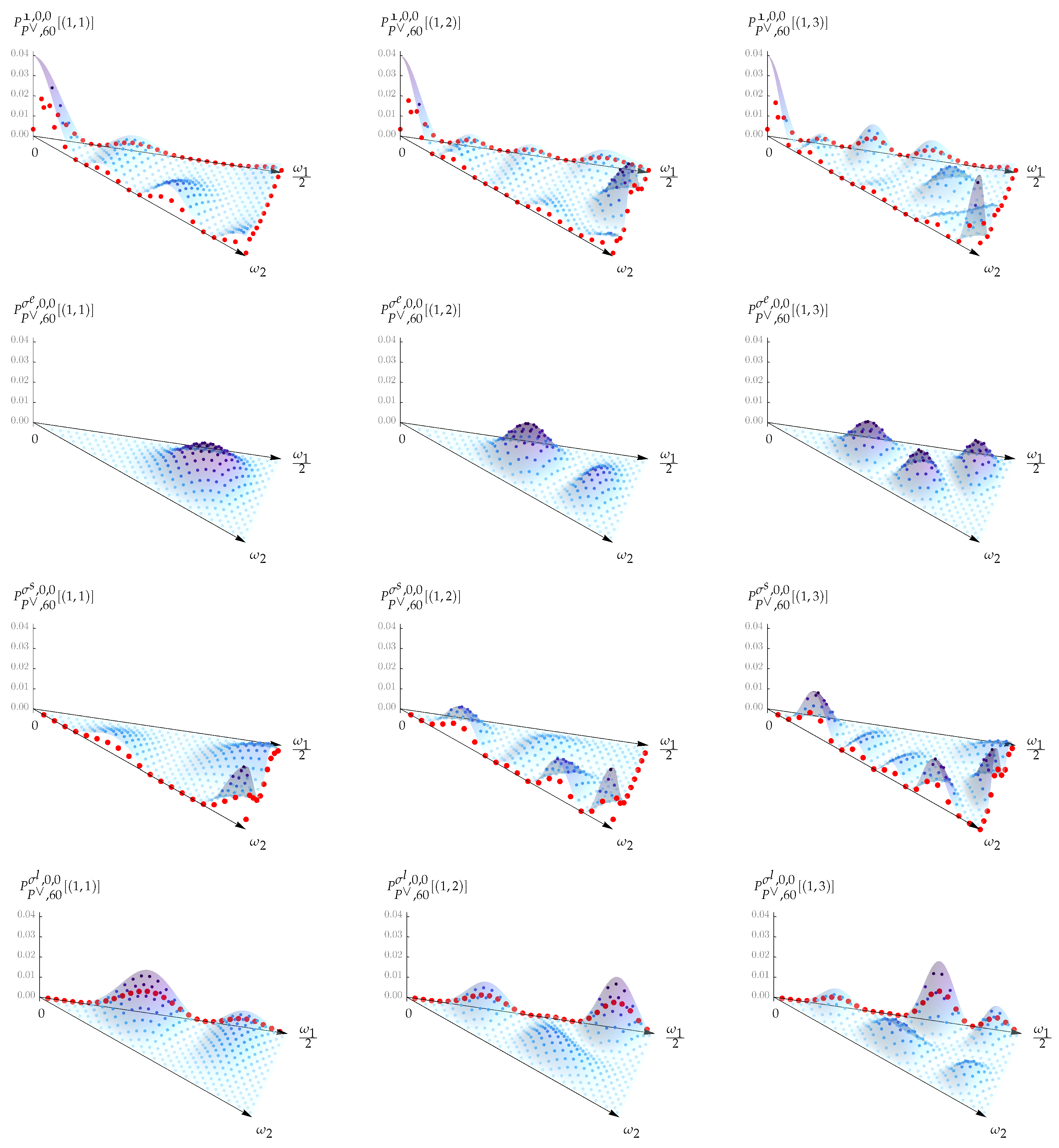
The probabilities $P_{P^{\vee },60}^{\sigma ,0,0}\left[\lambda \right]$ of finding the particle in several lower stationary states $|\lambda \rangle$ at the positions of the four dual-weight dots $a\in D_{P^{\vee },1,60}^{\sigma }(0,0)$, $\sigma \in \{\mathfrak{1},{\sigma }^e,{\sigma }^s,{\sigma }^l\}$ are depicted in Figure 6.

5. Conclusions

• The developed one-particle dual-weight discrete quantum billiard systems describe the non-relativistic quantum particle propagating on the dots $D_{P^{\vee },l,M}^{\sigma }(\varrho ,{\varrho }^{\vee })$, which comprise finitely-many positions located inside the scaled closure of the Weyl alcove $lF\subset {\mathbb{R}}^n$. The precise arrangements (15) and (16) of the Dirichlet and Neumann walls $l{H}^{\sigma }\left(\varrho \right)$ and $l{B}^{\sigma }\left(\varrho \right)$ that realise the quantum trapping of the particle and coincide with the dual-root billiards [1] constitute the boundaries of the simplex $lF$. Any predetermined admissible dual-weight hopping function ${\mathcal{P}}^{\vee }$, which encodes the amplitude propagation to the neighbouring positions, directly provides explicit formulas for the eigenenergies of the systems (59) via its Fourier transform by the symmetric Weyl orbit sums over its finite dominant support ${supp}^{+}\left({\mathcal{P}}^{\vee }\right)$. The vectors of the orthonormal momentum basis, $|\lambda \rangle \in {\mathcal{H}}_{P^{\vee },M}^{\sigma }(\varrho ,{\varrho }^{\vee })$, $\lambda \in {\Lambda }_{Q,M}^{\sigma }(\varrho ,{\varrho }^{\vee })$, determined independently on the dual-weight hopping function ${\mathcal{P}}^{\vee }$ by their explicit form (56) constitute solutions of the time-independent Schrödinger Equation (58). The time evolution of the dual-weight quantum systems from any normalised initial state vector given in the position basis |a〉, $a\in F_{P^{\vee },M}^{\sigma }(\varrho ,{\varrho }^{\vee })$ is exactly determined (71).
• The presence of the affine Weyl group orbits of the target positions $a^{\prime }\in F_{P^{\vee },M}^{\sigma }(\varrho ,{\varrho }^{\vee })$ in the coupling sets (51) represent the first essential symmetry component for implementing the interactions enforced by the boundaries of $lF$. Secondly, the addition of the sign $\chi$-function (13) values over the affine-reflected positions $W^{\mathrm{aff}}{a}^{\prime }$ in the coupling set $N_{p^{\vee },M}(a,a^{\prime })$ counts the number and type of amplitude reflections between the source position $a\in F_{P^{\vee },M}^{\sigma }(\varrho ,{\varrho }^{\vee })$ and the target position $a^{\prime }\in F_{P^{\vee },M}^{\sigma }(\varrho ,{\varrho }^{\vee })$. The $\chi$-function generalises the sign functions from [40] that are necessary for describing the Galois symmetries of Weyl orbit functions. The square roots of the stabiliser ε-functions (7) present as factors in defining relation of the dual-weight hopping operators ${\hat{A}}_{P^{\vee },M}^{\sigma }(\varrho ,{\varrho }^{\vee })$ matrix elements in the position basis (52) and manifest a direct consequence of the weighted discrete orthogonality relations (39). The ε-function subsequently straightforwardly regulates the probabilities (74) of finding the particle in a stationary state on the Neumann walls of the simplex $lF$. The Neumann boundary effect, which is observed similarly in dual-root models [1], is pointedly evident in Figure 3 and Figure 6.
• Considering an electron as the quantum particle propagating in the current discrete quantum systems, a novel class of the tight-binding models [3] with the electron propagating among atoms positioned at the points of the dual-weight dot $D_{P^{\vee },l,M}^{\sigma }(\varrho ,{\varrho }^{\vee })$ is obtained. The hopping integrals [15] between the coupled neighbouring positions in the atomic lattice, which might be estimated from theoretical considerations and/or fine-tuned experimentally, directly enter the present models as the values of the dual-weight hopping function ${\mathcal{P}}^{\vee }$. Analogously to the dual-root models, the physical interpretation of the dual-weight models coincides with the inductively developed electron propagation in a crystal lattice [41]. Since the dual-weight Fourier–Weyl transforms of the current one-dimensional $A_1$ model of a linear crystal specialise to the four types I–IV of the discrete cosine and sine transforms [18,25], the current stationary state vectors represent boundary-dependent (anti)symmetric alternatives to the periodic exponential solutions [41]. Moreover, the discrete Hamiltonian approach used for dual-weight and dual-root models produces strictly defined boundary-dependent forms of the energy spectra (59).
• Similarly to the dual-root models, the dual-weight models employ the generalised dual-weight Fourier–Weyl transforms (41) to construct the momentum basis (56) together with the stationary states (70) and time-evolutions (71). The utilisation of the weight lattice transforms [23] as well as the dual-weight E-transforms [42] for the description of analogous discrete quantum systems deserves further study. Potentially resulting in the generalisation of the present models to the prominent honeycomb-type (pseudo)lattices [17,32], the intricate composition of the weight and root lattice transforms demands a specific construction of extension coefficients of the extended Weyl orbit functions [43]. The calculation of the extension coefficients is determined by the desired form of product-to-sum decomposition formulas (33), which characterise the coupling of the considered (pseudo)lattice model. Since the extended Weyl orbit function approach potentially represents alternative description to the (pseudo)spinor wavefunctions approach [17], the Fourier–Weyl transforms induced by the extended Weyl orbit functions, together with the discrete symmetry analysis of the associated quantum systems, deserve further study.

References

- Brus, A.; Hrivnák, J.; Motlochová, L. Quantum particle on dual root lattice in Weyl alcove. J. Phys. A Math. Theor. 2021, 54, 095202. [Google Scholar] [CrossRef]
- Lindsay, D.M.; Wang, Y.; George, T.F. The Hückel model for small metal clusters. IV. Orbital properties and cohesive energies for model clusters of up to several hundred atoms. J. Clust. Sci. 1990, 1, 107–126. [Google Scholar] [CrossRef]
- Manninen, M. Models of Metal Clusters and Quantum Dots. In Atomic Clusters and Nanoparticles; Guet, C., Hobza, P., Speigelman, F., David, F., Eds.; Springer: Berlin/Heidelberg, Germany, 2001. [Google Scholar]
- Fernández-Hurtado, V.; Mur-Petit, J.; García-Ripoll, J.J.; Molina, R.A. Lattice scars: Surviving in an open discrete billiard. New J. Phys. 2014, 16, 035005. [Google Scholar] [CrossRef] [Green Version]
- Miao, F.; Wijeratne, S.; Zhang, Y.; Coskun, U.C.; Bao, W.; Lau, C.N. Phase-Coherent Transport in Graphene Quantum Billiards. Science 2007, 317, 1530–1533. [Google Scholar] [CrossRef] [Green Version]
- McDonald, S.W.; Kaufman, A.N. Wave chaos in the stadium: Statistical properties of short-wave solutions of the Helmholtz equation. Phys. Rev. A 1988, 37, 3067–3086. [Google Scholar] [CrossRef]
- Howard, P.J.; O’Mahony, P.F. The behaviour of resonances in Hecke triangular billiards under deformation. J. Phys. A Math. Theor. 2007, 40, 9275. [Google Scholar] [CrossRef]
- Spina, M.E.; Saraceno, M. Quantum spectra of triangular billiards on the sphere. J. Phys. A Math. Gen. 2001, 34, 2549. [Google Scholar] [CrossRef] [Green Version]
- Martins Quintela, M.F.C.; Lopes dos Santos, J.M.B. A polynomial approach to the spectrum of Dirac–Weyl polygonal Billiards. J. Phys. Condens. Matter 2021, 33, 035901. [Google Scholar] [CrossRef]
- Gaddah, W. A Lie group approach to the Schrödinger equation for a particle in an equilateral triangular infinite well. Eur. J. Phys. 2013, 34, 1175. [Google Scholar] [CrossRef]
- Gaddah, W. Exact solutions to the Dirac equation for equilateral triangular billiard systems. J. Phys. A Math. Theor. 2018, 51, 385304. [Google Scholar] [CrossRef]
- Schachner, H.C.; Obermair, G.M. Quantum billiards in the shape of right triangles. Z. Phys. B 1994, 95, 113–119. [Google Scholar] [CrossRef]
- Mandarino, A.; Linowski, T.; Życzkowski, K. Bipartite unitary gates and billiard dynamics in the Weyl chamber. Phys. Rev. A 2018, 98, 012335. [Google Scholar] [CrossRef] [Green Version]
- Krimer, D.O.; Khomeriki, R. Realization of discrete quantum billiards in a two-dimensional optical lattice. Phys. Rev. A 2011, 84, 041807. [Google Scholar] [CrossRef] [Green Version]
- Güçlü, A.D.; Potasz, P.; Korkusinski, M.; Hawrylak, P. Graphene Quantum Dots; Springer: Berlin/Heidelberg, Germany, 2014. [Google Scholar]
- Hrivnák, J.; Motlochová, L. Graphene Dots via Discretizations of Weyl-Orbit Functions. In Lie Theory and Its Applications in Physics, Proceedings of Lie Theory and Its Applications in Physics, Varna, Bulgaria, June 2019; Dobrev, V., Ed.; Springer: Singapore, 2020; pp. 407–413. [Google Scholar]
- Rozhkov, A.V.; Nori, F. Exact wave functions for an electron on a graphene triangular quantum dot. Phys. Rev. B 2010, 81, 155401. [Google Scholar] [CrossRef] [Green Version]
- Czyżycki, T.; Hrivnák, J. Generalized discrete orbit function transforms of affine Weyl groups. J. Math. Phys. 2014, 55, 113508. [Google Scholar] [CrossRef] [Green Version]
- Hrivnák, J.; Motlochová, L.; Patera, J. On discretization of tori of compact simple Lie groups II. J. Phys. A 2012, 45, 255201. [Google Scholar] [CrossRef]
- Hrivnák, J.; Patera, J. On discretization of tori of compact simple Lie groups. J. Phys. A Math. Theor. 2009, 42, 385208. [Google Scholar] [CrossRef] [Green Version]
- Czyżycki, T.; Hrivnák, J.; Motlochová, L. Generalized Dual-Root Lattice Transforms of Affine Weyl Groups. Symmetry 2020, 12, 1018. [Google Scholar] [CrossRef]
- Hrivnák, J.; Motlochová, L. Dual-root lattice discretization of Weyl orbit functions. J. Fourier Anal. Appl. 2019, 25, 2521–2569. [Google Scholar] [CrossRef] [Green Version]
- Hrivnák, J.; Walton, M.A. Weight-Lattice Discretization of Weyl-Orbit Functions. J. Math. Phys. 2016, 57, 083512. [Google Scholar] [CrossRef] [Green Version]
- Li, H.; Xu, Y. Discrete Fourier analysis on fundamental domain and simplex of Ad lattice in d-variables. J. Fourier Anal. Appl. 2010, 16, 383–433. [Google Scholar] [CrossRef]
- Britanak, V.; Rao, K.; Yip, P. Discrete Cosine and Sine Transforms: General Properties, Fast Algorithms and Integer Approximations; Elsevier/Academic Press: Amsterdam, The Netherlands, 2007. [Google Scholar]
- Humphreys, J.E. Reflection Groups and Coxeter Groups; Cambridge Studies in Advanced Mathematics 29; Cambridge University Press: Cambridge, UK, 1990. [Google Scholar]
- Moody, R.V.; Motlochová, L.; Patera, J. Gaussian cubature arising from hybrid characters of simple Lie groups. J. Fourier Anal. Appl. 2014, 20, 1257–1290. [Google Scholar] [CrossRef] [Green Version]
- Klimyk, A.U.; Patera, J. Orbit functions. SIGMA 2006, 2, 006. [Google Scholar]
- Montangero, S.; Frustaglia, D.; Calarco, T.; Fazio, R. Quantum billiards in optical lattices. Europhys. Lett. 2009, 88, 30006. [Google Scholar] [CrossRef] [Green Version]
- Alhassid, Y. The statistical theory of quantum dots. Rev. Mod. Phys. 2000, 72, 895–968. [Google Scholar] [CrossRef] [Green Version]
- Mounet, N.; Gibertini, M.; Schwaller, P.; Campi, D.; Merkys, A.; Marrazzo, A.; Sohier, T.; Castelli, I.E.; Cepellotti, A.; Pizzi, G.; et al. Two-dimensional materials from high-throughput computational exfoliation of experimentally known compounds. Nature Nanotech. 2018, 13, 246–252. [Google Scholar] [CrossRef] [Green Version]
- Drissi, L.B.; Saidi, E.H.; Bousmina, M. Graphene, Lattice Field Theory and Symmetries. J. Math. Phys. 2011, 52, 022306. [Google Scholar] [CrossRef]
- Bloch, I.; Dalibard, J.; Nascimbène, S. Quantum simulations with ultracold quantum gases. Nat. Phys. 2012, 8, 267–276. [Google Scholar] [CrossRef]
- Harshman, N.L.; Olshanii, M.; Dehkharghani, A.S.; Volosniev, A.G.; Jackson, S.G.; Zinner, N.T. Integrable Families of Hard-Core Particles with Unequal Masses in a One-Dimensional Harmonic Trap. Phys. Rev. X 2017, 7, 041001. [Google Scholar]
- Tolar, J.; Chadzitaskos, G. Feynman’s path integral and mutually unbiased bases. J. Phys. A Math. Theor. 2009, 42, 245306. [Google Scholar] [CrossRef]
- Politi, A.; Cryan, M.J.; Rarity, J.G.; Yu, S.; O’Brien, J.L. Silica-on-Silicon Waveguide Quantum Circuits. Science 2008, 320, 646–649. [Google Scholar] [CrossRef] [PubMed] [Green Version]
- Bourbaki, N. Groupes et Algèbres de Lie, Chapiters IV, V, VI; Hermann: Paris, France, 1968. [Google Scholar]
- Vinberg, E.B.; Onishchik, A.L. Lie Groups and Lie Algebras; Springer: New York, NY, USA, 1994. [Google Scholar]
- Klimyk, A.U.; Patera, J. Antisymmetric orbit functions. SIGMA 2007, 3, 023. [Google Scholar] [CrossRef] [Green Version]
- Hrivnák, J.; Walton, M.A. Discretized Weyl-orbit functions: Modified multiplication and Galois symmetry. J. Phys. A Math. Theor. 2015, 48, 175205. [Google Scholar] [CrossRef] [Green Version]
- Feynman, R.P.; Leighton, R.B.; Sand, M. The Feynman Lectures on Physics: Volume III; Basic Books: New York, NY, USA, 2010. [Google Scholar]
- Hrivnák, J.; Juránek, M. On E-Discretization of Tori of Compact Simple Lie Groups. II. J. Math. Phys. 2017, 58, 103504. [Google Scholar] [CrossRef] [Green Version]
- Hrivnák, J.; Motlochová, L. Discrete cosine and sine transforms generalized to honeycomb lattice. J. Math. Phys. 2018, 59, 063503. [Google Scholar] [CrossRef] [Green Version]
Figure 1.
The 3D plots of the energy functions (left panel) and (right panel) of . The grey triangle, which is placed at the zero energy level, represents the dual fundamental domain .
Figure 2.
The dot of . The light blue triangle represents the fundamental domain . The boundary black dashed lines represent the Dirichlet walls . The point set , representing possible positions of the quantum particle, is formed by the dark dots. The lines connecting the dots symbolise the nearest neighbour coupling characterised by the hopping operator .
Figure 3.
The probability plots for of . The dots display the probabilities (74) of finding the particle in the stationary states , and over their respective positions from , . The red dots illustrate probabilities over the particle’s positions on the Neumann walls.
Figure 4.
Figure 5.
The dot of . The light triangle depicts the fundamental domain and its boundary black dashed lines correspond to the Dirichlet walls and boundary black line to the Neumann wall . The point set , representing possible positions of the quantum particle, is formed by the dark dots. The lines connecting the dots symbolise the nearest neighbour coupling characterised by the hopping operator .
Figure 6.
Publisher’s Note: MDPI stays neutral with regard to jurisdictional claims in published maps and institutional affiliations. |
© 2021 by the authors. Licensee MDPI, Basel, Switzerland. This article is an open access article distributed under the terms and conditions of the Creative Commons Attribution (CC BY) license (https://creativecommons.org/licenses/by/4.0/).
Share and Cite
MDPI and ACS Style
Brus, A.; Hrivnák, J.; Motlochová, L. Quantum Particle on Dual Weight Lattice in Weyl Alcove. Symmetry 2021, 13, 1338. https://0-doi-org.brum.beds.ac.uk/10.3390/sym13081338
AMA Style
Brus A, Hrivnák J, Motlochová L. Quantum Particle on Dual Weight Lattice in Weyl Alcove. Symmetry. 2021; 13(8):1338. https://0-doi-org.brum.beds.ac.uk/10.3390/sym13081338
Chicago/Turabian StyleBrus, Adam, Jiří Hrivnák, and Lenka Motlochová. 2021. "Quantum Particle on Dual Weight Lattice in Weyl Alcove" Symmetry 13, no. 8: 1338. https://0-doi-org.brum.beds.ac.uk/10.3390/sym13081338
Note that from the first issue of 2016, this journal uses article numbers instead of page numbers. See further details here.