A Multivariate Flexible Skew-Symmetric-Normal Distribution: Scale-Shape Mixtures and Parameter Estimation via Selection Representation

Abstract

Multivariate skew-symmetric-normal (MSSN) distributions have been recognized as an appealing tool for modeling data with non-normal features such as asymmetry and heavy tails, rendering them suitable for applications in diverse areas. We introduce a richer class of MSSN distributions based on a scale-shape mixture of (multivariate) flexible skew-symmetric normal distributions, called the SSMFSSN distributions. This very general class of SSMFSSN distributions can capture various shapes of multimodality, skewness, and leptokurtic behavior in the data. We investigate some of its probabilistic characterizations and distributional properties which are useful for further methodological developments. An efficient EM-type algorithm designed under the selection mechanism is advocated to compute the maximum likelihood (ML) estimates of parameters. Simulation studies as well as applications to a real dataset are employed to illustrate the usefulness of the presented methods. Numerical results show the superiority of our proposed model in comparison to several existing competitors.

1. Introduction

The use of multivariate normal (MN) distribution plays a central role in statistical modeling. However, there are some situations where the data are not in agreement with the MN distribution. Departure from normality can take place in different ways, such as multimodality, lack in central symmetry, and positive or negative excess of kurtosis. The class of scale mixtures of skew-normal distributions (SMSN) whose general form was first introduced by Branco and Dey [1] includes many multivariate skew symmetric (MSS) distributions with only one mode.

More formally, a scale mixture distribution can be constituted by mixing a base density over a scaling distribution. Its density can be expressed in the form of the integral given by

$$f\left(\mathit{y}\right)={\int }_0^{\infty }g\left(\mathit{y}\left|\kappa \right(\tau )\right)dH(\tau ;\mathbf{\nu }),$$

(1)

where $g\left(\mathit{y}\left|\kappa \right(\tau )\right)$ is the conditional density of a $p\times 1$ random vector $\mathit{Y}$ given $\kappa \left(\tau \right)$. Herein, $\kappa (·)$ is a positive function of a scaling variable $\tau$ with cumulative distribution function (cdf) $H(\tau ;\mathbf{\nu })$, indexed by the parameter vector $\mathbf{\nu }$.

Using (1), the family of SMSN distributions can be generated by assuming a multivariate skew-normal (MSN) distribution [2] with location $\mathbf{\xi }$, scale covariance matrix $\kappa \left(\tau \right)\mathsf{\Sigma }$, and shape parameter $\mathbf{\lambda }$ for $g\left(\mathit{y}\left|\kappa \right(\tau )\right)$. The marginal probability density function (pdf) of $\mathit{Y}$ can be obtained as follows:

$$\begin{array}{c}\hfill f\left(\mathit{y}\right)=2{\int }_0^{\infty }{\varphi }_p(\mathit{y};\mathbf{\xi },\kappa \left(\tau \right)\mathsf{\Sigma })\mathsf{\Phi }\left(\kappa {\left(\tau \right)}^{-1/2}{\mathbf{\lambda }}^{\top }{\mathsf{\Sigma }}^{-1/2}(\mathit{y}-\mathbf{\xi })\right)dH(\tau ;\mathbf{\nu }),\end{array}$$

(2)

where ${\varphi }_p(·;\mathbf{\xi },\mathsf{\Sigma })$ denotes the pdf of the p-variate MN distribution with mean vector $\mathbf{\xi }$ and covariance matrix $\mathsf{\Sigma }$, and $\mathsf{\Phi }(·)$ is the cdf of the standard normal distribution. Some simple scaling functions such as $\kappa \left(\tau \right)=\tau$ and $\kappa \left(\tau \right)=1/\tau$ lead to well-known distributions. As described by Branco and Dey [1], some remarkable examples are the multivariate skew-t (MST), multivariate skew-slash (MSSL), and multivariate skew-contaminated-normal (MSCN) distributions, to name just a few. The SMSN family collapses to the class of scale mixture of normal distributions when the skewness parameter vanishes. The MSN distribution [2] with the parameterization given by Arellano-Valle and Genton [3] can be recovered when $H(\tau ;\mathbf{\nu })$ is degenerated by imposing $\tau =1$.

The multivariate skew-scale mixtures of normal (MSSMN) distributions [4] is established when $g\left(\mathit{y}\left|\kappa \right(\tau )\right)$ defined in (1) is given by

$$\begin{array}{c}\hfill g\left(\mathit{y}|\kappa \left(\tau \right)={\tau }^{-1}\right)=2{\varphi }_p(\mathit{y};\mathbf{\xi },{\tau }^{-1}\mathsf{\Sigma })\mathsf{\Phi }\left({\mathbf{\lambda }}^{\top }{\mathsf{\Sigma }}^{-1/2}(\mathit{y}-\mathbf{\xi })\right).\end{array}$$

(3)

Therefore, the pdf of MSSMN distribution is obtained as follows:

$$\begin{array}{c}\hfill f\left(\mathit{y}\right)=2\mathsf{\Phi }\left({\mathbf{\lambda }}^{\top }{\mathsf{\Sigma }}^{-1/2}(\mathit{y}-\mathbf{\xi })\right){\int }_0^{\infty }{\varphi }_p(\mathit{y};\mathbf{\xi },{\tau }^{-1}\mathsf{\Sigma })dH(\tau ;\mathbf{\nu }).\end{array}$$

(4)

Recently, Arellano-Valle et al. [5] proposed a multivariate class of scale-shape mixtures of skew-normal (MSSMSN) distributions which provides alternative candidates for modeling asymmetric data. A convenient hierarchical representation of the MSSMSN distribution is given by

$$\mathit{Y}|\mathbf{\tau }={({\tau }_1,{\tau }_2)}^{\top }\sim S{N}_p\left(\mathbf{\xi },\kappa \left({\tau }_1\right)\mathsf{\Sigma },\eta ({\tau }_1,{\tau }_2)\mathbf{\lambda }\right),$$

(5)

where $\mathbf{\tau }={({\tau }_1,{\tau }_2)}^{\top }$ is a mixing vector with a joint cdf $H({\tau }_1,{\tau }_2;\mathbf{\nu })$, and $\eta ({\tau }_1,{\tau }_2):({\mathbb{R}}^{+},{\mathbb{R}}^{+})\to \mathbb{R}$ is a real-valued shape mixing function which is not necessarily symmetric about zero. The family of MSSMSN distributions encapsulates several renowned unimodal asymmetric distributions generated by varying the scale and shape functions, $\kappa \left({\tau }_1\right)$ and $\eta ({\tau }_1,{\tau }_2)$, for a given distribution of $\mathbf{\tau }$, or alternatively by fixing $\kappa \left({\tau }_1\right)$ and $\eta ({\tau }_1,{\tau }_2)$ but varying the distribution of $\mathbf{\tau }$. A convenient setup for the mixing functions is to choose $\kappa \left({\tau }_1\right)=1/{\tau }_1$ and $\eta ({\tau }_1,{\tau }_2)=\sqrt{{\tau }_2}$, leading to a particular form of the shape mixture of SMSN distributions. If we choose $\eta ({\tau }_1,{\tau }_2)={({\tau }_1/{\tau }_2)}^{-1/2}$, it produces another form of shape mixtures of MSSMN distributions. See [5] for a more comprehensive discussion and detailed investigation.

As shown by Azzalini and Capitanio [6], the pdf of the MSS distribution can be written as follows:

$$f(\mathit{y};\mathbf{\xi },\mathsf{\Sigma })={2\left|\mathsf{\Sigma }\right|}^{-1/2}{f}_0\left({\mathsf{\Sigma }}^{-1/2}(\mathit{y}-\mathbf{\xi })\right)G_0\left(w\left\{{\mathsf{\Sigma }}^{-1/2}(\mathit{y}-\mathbf{\xi })\right\}\right),$$

(6)

where $\mathbf{\xi }$ and $\mathsf{\Sigma }$ are, respectively, the location vector and scale covariance matrix; $f_0:{\mathbb{R}}^p\to {\mathbb{R}}^{+}$ is a p-variate centrally symmetric pdf with respect to the origin, i.e., $f_0\left(\mathit{x}\right)=f_0(-\mathit{x})$; $G_0:\mathbb{R}\to [0,1]$ is a univariate cdf satisfying $G_0(-x)=1-G_0\left(x\right)$; and $w:{\mathbb{R}}^p\to \mathbb{R}$ is an odd real-valued function, namely $w\{-\mathit{x}\}=w\left\{\mathit{x}\right\}$. The MSS class is equivalent to the one studied by Wang et al. [7] for which $G_0\left(w\left\{\mathit{x}\right\}\right)$ is replaced by $\pi :{\mathbb{R}}^p\to [0,1]$ satisfying $\pi (-\mathit{x})=1-\pi \left(\mathit{x}\right)$.

In light of (6), it is possible to generate a wide range of asymmetric families of unimodal and multimodal skew distributions depending on the specification of the function $w\left\{\mathit{x}\right\}$. This essential property induces greater flexibility in the available shapes. For example, Ma and Genton [8] proposed a flexible class of skew-symmetric distributions by choosing $w\left\{\mathit{x}\right\}=P_K\left(\mathit{x}\right)$, where $P_K\left(\mathit{x}\right)$ is an odd polynomial function of order K.

The Hadamard product, also known as the Schur product, is a type of matrix multiplication that is commutative and simpler than the matrix product. See [9] for a comprehensive review and its applications to multivariate statistical analysis. The Hadamard product is advantageous in computations and algebraic manipulations because the products are entry-wise, the multiplication is commutative, and, particularly, the inverse is very easy to obtain and the computation of power matrices is straightforward. By convention, we use “⊙" to denote the Hadamard operations (product and power). Let $\mathit{A}=\left(a_{ij}\right)$ and $\mathit{B}=\left(b_{ij}\right)$ be two $p\times q$ matrices of the same dimension but not necessarily square. Then, the Hadamard product between these two matrices, denoted by $\mathit{A}\odot \mathit{B}$, is the element-wise product of $\mathit{A}$ and $\mathit{B}$, that is, a $p\times q$ matrix whose $(i,j)$ entry is $a_{ij}{b}_{ij}$. Accordingly, the nth Hadamard power of matrix $\mathit{A}$ is defined as ${\mathit{A}}^{\odot n}=\left[a_{ij}^n\right]$. More key properties concerning the multiplication and partial derivatives of the Hadamard product are deferred to Appendix A.

In the multivariate setup, the odd polynomial of order K has various combinations of the coefficients. For example, the bivariate case under an odd polynomial of order $K=3$ is given by $P_K(x_1,x_2)={\alpha }_1{x}_1+{\alpha }_2{x}_2+{\alpha }_3{x}_1^3+{\alpha }_4{x}_2^3+{\alpha }_5{x}_1^2{x}_2+{\alpha }_6{x}_1{x}_2^2$. As an alternative to that of Ma and Genton [8] in more a general setting, we introduce the multivariate flexible skew-symmetric-normal (MFSSN) distribution, denoted by $MFSS{N}_p(\mathbf{\xi },\mathsf{\Sigma },\mathbf{\alpha })$, which has the following pdf:

$$\begin{array}{c}\hfill f_{MFSSN}(\mathit{y};\mathbf{\xi },\mathsf{\Sigma },\mathbf{\alpha })=2{\varphi }_p(\mathit{y};\mathbf{\xi },\mathsf{\Sigma })\mathsf{\Phi }\left({\mathbf{\lambda }}_1^{\top }{\mathbf{\eta }}_1+{\mathbf{\lambda }}_2^{\top }{\mathbf{\eta }}_3+\cdots +{\mathbf{\lambda }}_m^{\top }{\mathbf{\eta }}_{2m-1}\right),\end{array}$$

(7)

where $\mathbf{\alpha }={({\mathbf{\lambda }}_1^{\top },\dots ,{\mathbf{\lambda }}_m^{\top })}^{\top }$ is a $pm\times 1$ multiple-scaled vector of shape parameters and ${\mathbf{\eta }}_{2k-1}={\left[{\mathsf{\Sigma }}^{-1/2}(\mathit{y}-\mathbf{\xi })\right]}^{\odot 2k-1}$ remains a $p\times 1$ vector through an odd Hadamard power transformation of order $2K-1$, for $K=1,\dots ,m$. Notably, the MFSSN distribution encompasses the flexible generalized skew-normal (FGSN) distribution introduced by Ma and Genton [8] as the univariate case. Figure 1 illustrates the scatter-contour plots coupled with their marginal histograms of the bivariate MFSSN distribution under $\mathbf{\xi }=\mathbf{0}$, $\mathsf{\Sigma }={\mathit{I}}_2$ and various specifications of shape parameters arisen from two setups of m. As can be seen, many different non-elliptically distributional shapes with multiple modes and asymmetric patterns can be produced. Additional flexibility can be gained by expanding the thickness of tails. This motivates us to propose a more general class of scale-shape mixtures of MFSSN (SSMFSSN) distributions.

The class of SSMFSSN distributions can be hierarchically represented by

$$\begin{array}{c}\hfill \mathit{Y}\mid \mathbf{\tau }={({\tau }_1,{\tau }_2)}^{\top }\sim MFSS{N}_p(\mathbf{\xi },{\tau }_1^{-1}\mathsf{\Sigma },\mathbf{\vartheta }),\end{array}$$

(8)

where $\mathbf{\vartheta }={\left({\mathbf{\lambda }}_1^{\top }{\tau }_2^{1/2}{\tau }_1^{-1/2},\cdots ,{\mathbf{\lambda }}_m^{\top }{\tau }_2^{1/2}{\tau }_1^{-(2m-1)/2}\right)}^{\top }$. Further, we denote the pdf of $\mathbf{\tau }={({\tau }_1,{\tau }_2)}^{\top }$ by $h_{\mathbf{\tau }}({\tau }_1,{\tau }_2;\mathbf{\nu })$. From (8), the marginal pdf of $\mathit{Y}$ is given by

$$\begin{array}{ccc}\hfill f_{SSMFSSN}(\mathit{y};\mathbf{\xi },\mathsf{\Sigma },\mathbf{\zeta },\mathbf{\nu })& =& \int {\varphi }_p(\mathit{y};\mathbf{\xi },{\tau }_1^{-1}\mathsf{\Sigma })\mathsf{\Phi }({\tau }_2^{1/2}\{{\mathbf{\lambda }}_1^{\top }{\mathbf{\eta }}_1+{\mathbf{\lambda }}_2^{\top }{\mathbf{\eta }}_3\hfill \\ & & +\cdots +{\mathbf{\lambda }}_m^{\top }{\mathbf{\eta }}_{2m-1}\left\}\right)dH(\mathbf{\tau };\mathbf{\nu }).\hfill \end{array}$$

(9)

Obviously, the MFSSN model is obtained by setting ${\tau }_1={\tau }_2=1$ in (9).

The family of SSMFSSN distributions introduced in (8) is quite vast, containing several subfamilies of asymmetric and multimodal distributions which have never been considered in the literature. Notice that the MSSMSN distribution described in (5) is a simple case of SSMFSSN by taking $\kappa \left({\tau }_1\right)=1/{\tau }_1$, $\eta ({\tau }_1,{\tau }_2)={({\tau }_1/{\tau }_2)}^{-1/2}$, and ${\mathbf{\lambda }}_j=\mathbf{0}$, for $j=2,\dots ,m$. More importantly, the scale-shape mixtures of flexible generalized skew-normal (SSMFGSN) distributions proposed very recently by Mahdavi et al. [10] can be thought of as a univariate case of SSMFSSN when the dimension $p=1$.

The EM algorithm [11] and some of its extraordinary variants such as the expectation conditional maximization (ECM) algorithm [12] and the expectation conditional maximization either (ECME) algorithm [13] are broadly applicable methods to carry out ML estimation for multivariate skew distributions in a complete-data framework. To the best of our knowledge, previous developments of the EM-type algorithm are based on the convolution-type representations, see, e.g., [14] for the MSN distribution, [15] for the MST distribution, [1] for the SMSN distribution, and [5] for the MSSMSN distribution. Since our proposed SSMFSSN model cannot be explicitly expressed by a convolution-type representation, we develop a novel EM-based procedure designed under the selection mechanism to compute the ML estimates.

The rest of the paper is organized as follows. Section 2 presents the formulation of the general SSMFSSN model and discusses how to deploy the ECME algorithm for ML estimation based on the selection-type mechanism. Section 3 exemplifies some particular cases of SSMFSSN distributions constructed by setting different mixing distributions for $\mathbf{\tau }$. The proposed techniques are illustrated by conducting two simulation studies in Section 4 and analyzing a real data example in Section 5. We conclude in Section 6 with a few remaks and offer directions for future research.

2. Methodology

2.1. The Family of SSMFSSN Distributions

A p-variate random vector $\mathit{Y}$∼$SSMFSS{N}_p(\mathbf{\xi },\mathsf{\Sigma },\mathbf{\alpha },\mathbf{\nu })$ is asserted to follow the SSMFSSN distribution with location vector $\mathbf{\xi }$, scale covariance matrix $\mathsf{\Sigma }$, shape parameters $\mathbf{\alpha }={({\mathbf{\lambda }}_1^{\top },\dots ,{\mathbf{\lambda }}_m^{\top })}^{\top }$, and flatness parameters $\mathbf{\nu }$ if it has the following selection-type representation:

$$\begin{array}{c}\hfill \mathit{Y}\stackrel{d}{=}\mathit{V}\mid (U>0),\end{array}$$

(10)

where $\mathit{V}=\mathbf{\xi }+{\mathsf{\Sigma }}^{1/2}{\tau }_1^{-1/2}{\mathit{Z}}_1$, $U={\mathbf{\lambda }}_1^{\top }\left({\tau }_1^{-1/2}{\mathit{Z}}_1\right)+\cdots +{\mathbf{\lambda }}_m^{\top }\left({\tau }_1^{-(2m-1)/2}{\mathit{Z}}_1^{\odot 2m-1}\right)-{\tau }_2^{-1/2}{Z}_2$ and ${({\mathit{Z}}_1^{\top },Z_2)}^{\top }$∼$N_{p+1}(\mathbf{0},{\mathit{I}}_{p+1})$. Herein, ‘$\stackrel{d}{=}$’ stands for equality in distribution, and U is obviously a continuous random variable symmetric about zero. Using this characterization, the random samples for $SSMFSS{N}_p(\mathbf{0},{\mathit{I}}_p,\mathbf{\alpha },\mathbf{\nu })$ can be simulated through the following scheme

$$\begin{array}{c}\hfill \mathit{X}=\left\{\begin{array}{c}{\tau }_1^{-1/2}{\mathit{Z}}_1,\mathrm{if}U>0,\\ -{\tau }_1^{-1/2}{\mathit{Z}}_1,\mathrm{otherwise}.\end{array}\right.\end{array}$$

(11)

As a result, the random samples of the general $SSMFSS{N}_p(\mathbf{\xi },\mathsf{\Sigma },\mathbf{\alpha },\mathbf{\nu })$ can be obtained by the affine transformation $\mathit{Y}=\mathbf{\xi }+{\mathsf{\Sigma }}^{1/2}\mathit{X}$.

For fitting the SSMFSSN model (10) within the complete-data framework via the EM-type algorithm, we introduce two latent variables $W\stackrel{d}{=}U\mid (U>0)$ and $\mathbf{\gamma }={({\gamma }_1,{\gamma }_2)}^{\top }\stackrel{d}{=}{({\tau }_1,{\tau }_2)}^{\top }\mid (U>0)$. Then, ${({\mathit{Y}}^{\top },W,{\mathbf{\gamma }}^{\top })}^{\top }\stackrel{d}{=}{({\mathit{V}}^{\top },U,{\mathbf{\tau }}^{\top })}^{\top }|(U>0)$ has the following joint pdf:

$$\begin{array}{ccc}\hfill f_{\mathit{Y},W,\mathbf{\gamma }}(\mathit{y},W,\mathbf{\gamma })& =& \frac{1}{Pr(U>0)}{f}_{\mathit{V},U,\mathbf{\tau }}(\mathit{y},W,\mathbf{\gamma })\hfill \\ & =& 2f_{\mathbf{\tau }}\left(\mathbf{\gamma }\right)f_{\mathit{V}|\mathbf{\tau }}\left(\mathit{y}\right)f_{U|\mathit{V},\mathbf{\tau }}\left(W\right)\hfill \\ & =& 2{\gamma }_2^{1/2}{h}_{\mathbf{\tau }}({\gamma }_1,{\gamma }_2;\mathbf{\nu }){\varphi }_p\left(\mathit{y};\mathbf{\xi },{\gamma }_1^{-1}\mathsf{\Sigma }\right)\varphi \left({\gamma }_2^{1/2}\{W-\zeta \}\right),\hfill \end{array}$$

(12)

where $\zeta ={\mathbf{\lambda }}_1^{\top }{\mathbf{\eta }}_1+\cdots +{\mathbf{\lambda }}_m^{\top }{\mathbf{\eta }}_{2m-1}$, $h_{\mathbf{\tau }}({\gamma }_1,{\gamma }_2;\mathbf{\nu })$ is the pdf of $\mathbf{\tau }={({\tau }_1,{\tau }_2)}^{\top }$ evaluated at point $\mathbf{\gamma }={({\gamma }_1,{\gamma }_2)}^{\top }$.

Integrating out W from (12) gives the following joint pdf

$$\begin{array}{ccc}\hfill f_{\mathit{Y},\mathbf{\gamma }}(\mathit{y},{\gamma }_1,{\gamma }_2)& =& 2h_{\mathbf{\tau }}({\gamma }_1,{\gamma }_2;\mathbf{\nu }){\varphi }_p\left(\mathit{y};\mathbf{\xi },{\gamma }_1^{-1}\mathsf{\Sigma }\right)\mathsf{\Phi }\left({\gamma }_2^{1/2}\zeta \right).\hfill \end{array}$$

(13)

Therefore, the marginal pdf of $\mathit{Y}$ is given by

$$\begin{array}{ccc}\hfill f_{\mathit{Y}}\left(\mathit{y}\right)& =& {\int }_0^{\infty }{\int }_0^{\infty }{f}_{\mathit{Y},\mathbf{\gamma }}(\mathit{y},{\gamma }_1,{\gamma }_2)d{\gamma }_{1}d{\gamma }_2\hfill \\ & \stackrel{{\tau }_1\perp {\tau }_2}{=}& 2\int {\varphi }_p(\mathit{y};\mathbf{\xi },{\gamma }_1^{-1}\mathsf{\Sigma })d{H}_{{\tau }_1}({\gamma }_1;{\mathbf{\nu }}_1)\int \mathsf{\Phi }\left({\gamma }_2^{1/2}\zeta \right)d{H}_{{\tau }_2}({\tau }_2;{\mathbf{\nu }}_2),\hfill \end{array}$$

(14)

where the second equality holds if we further assume ${\tau }_1$ and ${\tau }_2$ are mutually independent. It is noteworthy that the shape mixtures of MSSMN distribution established by Arellano-Valle et al. [5] also belongs to the family of our proposed SSMFSSN model by imposing ${\mathbf{\lambda }}_2=\cdots ={\mathbf{\lambda }}_m=\mathbf{0}$.

Dividing (12) by (13) yields the following relation

$$\begin{array}{ccc}\hfill f(W\mid \mathit{y},{\gamma }_1,{\gamma }_2)& =& \frac{{\gamma }_2^{1/2}\varphi \left({\gamma }_2^{1/2}(W-\zeta )\right)}{\mathsf{\Phi }\left({\gamma }_2^{1/2}\zeta \right)}\equiv f(W\mid \mathit{y},{\gamma }_2),\hfill \end{array}$$

(15)

for which ‘≡’ in (15) means that W and ${\gamma }_1$ are conditionally independent. Moreover, it is straightforward to show that

$$W\mid {({\mathit{y}}^{\top },{\gamma }_2)}^{\top }\sim TN\left(\zeta ,{\gamma }_2^{-1}\right)I_{(0,\infty )},$$

(16)

where $TN(\mu ,{\sigma }^2)I_{\mathbb{A}}$ represents a doubly truncated normal distribution confined within the interval $\mathbb{A}=\{a_1<x<a_2\}$, and $I_{\mathbb{A}}$ is an indicator function of set $\mathbb{A}$. Using Lemma 2 of Lin et al. [16], we have the following conditional expectation:

$$E(W\mid \mathit{y},{\gamma }_2)=\zeta +{\gamma }_2^{-1/2}\frac{\varphi \left({\gamma }^{1/2}\zeta \right)}{\mathsf{\Phi }\left({\gamma }^{1/2}\zeta \right)}.$$

(17)

By Bayes’ rule, the conditional pdf of $\mathbf{\gamma }={({\gamma }_1,{\gamma }_2)}^{\top }$ given $\mathit{Y}=\mathit{y}$ is

$$\begin{array}{c}\hfill f({\gamma }_1,{\gamma }_2\mid \mathit{y})=\frac{2h_{\mathbf{\tau }}({\gamma }_1,{\gamma }_2;\mathbf{\nu }){\varphi }_p\left(\mathit{y};\mathbf{\xi },{\gamma }_1^{-1}\mathsf{\Sigma }\right)\mathsf{\Phi }\left({\gamma }_2^{1/2}\zeta \right)}{f_{\mathit{Y}}\left(\mathit{y}\right)}.\end{array}$$

(18)

2.2. Parameter Estimation via the ECME Algorithm

The EM algorithm [11] is a widely used iterative technique to deal with ML estimation in models that involve incomplete data or latent variables. One primary virtue of EM lies in the fact of attractive monotone convergence properties and the preservation of simplicity and stability. In practice, a major limitation of EM is often that some estimators in the M-step cannot be solved in terms of closed-form expressions. To overcome this obstacle, the ECM algorithm proposed by Meng and Rubin [12] recommends replacing the E-step of EM with a sequence of simpler conditional maximization (CM) steps, yet it also enjoys the same convergence properties as EM. However, in certain problems, some of the CM-steps of ECM may become analytically intractable or suffer from slow convergence. As a further flexible extension, the ECME algorithm [13] divides the CM-steps of ECM to maximize either the Q-function, called the CMQ-step, or the corresponding constrained actual log-likelihood function, named as the CML-step. In what follows, we describe in greater detail how the proposed SSMFSSN model can be fitted by using the ECME algorithm.

Suppose that $\mathit{y}={({\mathit{y}}_1^{\top },\dots ,{\mathit{y}}_n^{\top })}^{\top }$ constitutes a set of p-dimensional observed samples of size n arising from the SSMFSSN model. Under the EM framework, the latent variables $\mathit{W}={(W_1,\dots ,W_n)}^{\top }$ and $\mathbf{\gamma }={({\mathbf{\gamma }}_1^{\top },\dots ,{\mathbf{\gamma }}_n^{\top })}^{\top }$ introduced in the preceding subsection are treated as missing data. Then, the complete data are given by ${\mathit{y}}_c={({\mathit{y}}^{\top },{\mathit{W}}^{\top },{\mathbf{\gamma }}^{\top })}^{\top }$. Further, we let $\mathbf{\theta }={({\mathbf{\xi }}^{\top },\mathrm{vech}{\left(\mathsf{\Sigma }\right)}^{\top },{\mathbf{\alpha }}^{\top },{\mathbf{\nu }}^{\top })}^{\top }$ denote the entire unknown parameters to be estimated in the SSMFSSN model, where $\mathrm{vech}(·)$ is the half-vectorization operator that stacks the lower triangular elements of a $p\times p$ symmetric matrix into a single $p(p+1)/2$ vector.

According to (12), the log-likelihood function of $\mathbf{\theta }$ corresponding to the complete-data ${\mathit{y}}_c$, excluding additive constants and terms that do not involve parameters of the model, is given by

$$\begin{array}{ccc}\hfill {\ell }_c(\mathbf{\theta }\mid {\mathit{y}}_c)& =& -\frac{n}{2}ln\left|\mathsf{\Sigma }\right|-\frac{1}{2}\sum _{i=1}^n\{{\gamma }_{1i}{({\mathit{y}}_i-\mathbf{\xi })}^{\top }{\mathsf{\Sigma }}^{-1}({\mathit{y}}_i-\mathbf{\xi })+{\gamma }_{2i}{(W_i-{\zeta }_i)}^2\hfill \\ & & -2lnh({\gamma }_{1i},{\gamma }_{2i};\mathbf{\nu })\},\hfill \end{array}$$

(19)

with

$$\begin{array}{ccc}\hfill {\zeta }_i& =& {\mathbf{\lambda }}_1^{\top }{\mathbf{\eta }}_{i,1}+{\mathbf{\lambda }}_2^{\top }{\mathbf{\eta }}_{i,3}+\cdots +{\mathbf{\lambda }}_m^{\top }{\mathbf{\eta }}_{i,2m-1},\hfill \\ & =& {\mathbf{\lambda }}_1^{\top }{\left[{\mathsf{\Sigma }}^{-1/2}({\mathit{y}}_i-\mathbf{\xi })\right]}^{\odot 1}+{\mathbf{\lambda }}_2^{\top }{\left[{\mathsf{\Sigma }}^{-1/2}({\mathit{y}}_i-\mathbf{\xi })\right]}^{\odot 3}+\cdots +{\mathbf{\lambda }}_m^{\top }{\left[{\mathsf{\Sigma }}^{-1/2}({\mathit{y}}_i-\mathbf{\xi })\right]}^{\odot 2m-1}\hfill \\ & =& {\mathbf{1}}_p^{\top }{\mathsf{\Lambda }}_1{\left[{\mathsf{\Sigma }}^{-1/2}({\mathit{y}}_i-\mathbf{\xi })\right]}^{\odot 1}+{\mathbf{1}}_p^{\top }{\mathsf{\Lambda }}_2{\left[{\mathsf{\Sigma }}^{-1/2}({\mathit{y}}_i-\mathbf{\xi })\right]}^{\odot 3}+\cdots +{\mathbf{1}}_p^{\top }{\mathsf{\Lambda }}_m{\left[{\mathsf{\Sigma }}^{-1/2}({\mathit{y}}_i-\mathbf{\xi })\right]}^{\odot 2m-1}\hfill \\ & =& {\mathbf{1}}_p^{\top }{\left[{\Delta }_1({\mathit{y}}_i-\mathbf{\xi })\right]}^{\odot 1}+{\mathbf{1}}_p^{\top }{\left[{\Delta }_2({\mathit{y}}_i-\mathbf{\xi })\right]}^{\odot 3}+\cdots +{\mathbf{1}}_p^{\top }{\left[{\Delta }_m({\mathit{y}}_i-\mathbf{\xi })\right]}^{\odot 2m-1}\hfill \\ & =& {\mathbf{1}}_p^{\top }\sum _{j=1}^m{\left[{\Delta }_j({\mathit{y}}_i-\mathbf{\xi })\right]}^{\odot 2j-1},\hfill \end{array}$$

where ${\mathbf{1}}_p$ is a $p\times 1$ vector of ones, ${\mathbf{\eta }}_{i,2j-1}={\left[{\mathsf{\Sigma }}^{-1/2}({\mathit{y}}_i-\mathbf{\xi })\right]}^{\odot 2j-1}$, ${\mathsf{\Lambda }}_j=\mathrm{Diag}\left\{{\mathbf{\lambda }}_j\right\}$ is a $p\times p$ diagonal matrix containing the elements of ${\mathbf{\lambda }}_j$ on the main diagonal, and ${\Delta }_j={\mathsf{\Lambda }}_j^{1/(2j-1)}{\mathsf{\Sigma }}^{-1/2}$ is a $p\times p$ reparameterized matrix.

On the kth iteration, the E-step requires the calculation of the so-called Q-function, which is the conditional expectation of (19) given the observed data $\mathit{y}$ and the current estimate ${\widehat{\mathbf{\theta }}}^{\left(k\right)}$, where the superscript ${}^{\left(k\right)}$ denote the updated estimates at iteration k. To evaluate the Q-function, we require the following conditional expectations:

$$\begin{array}{c}\hfill {\widehat{s}}_{1i}^{\left(k\right)}=E({\gamma }_{1i}\mid {\mathit{y}}_i,{\widehat{\mathbf{\theta }}}^{\left(k\right)}),{\widehat{s}}_{2i}^{\left(k\right)}=E({\gamma }_{2i}\mid {\mathit{y}}_i,{\widehat{\mathbf{\theta }}}^{\left(k\right)}),{\widehat{s}}_{3i}^{\left(k\right)}=E(W_i{\gamma }_{2i}\mid {\mathit{y}}_i,{\widehat{\mathbf{\theta }}}^{\left(k\right)}),\end{array}$$

(20)

which have explicit expressions that are discussed in detail in a subsequent section along with

$${\widehat{s}}_{4i}^{\left(k\right)}\left(\mathbf{\nu }\right)=E(lnh({\gamma }_{1i},{\gamma }_{2i};\mathbf{\nu })\mid {\mathit{y}}_i,{\widehat{\mathbf{\theta }}}^{\left(k\right)}),$$

(21)

which may not have standard form for some subfamilies. Substituting (20) and (21) into (19) yields the following Q-function:

$$\begin{array}{ccc}\hfill Q(\mathbf{\theta }\mid {\widehat{\mathbf{\theta }}}^{\left(k\right)})& =& -\frac{n}{2}ln\left|\mathsf{\Sigma }\right|-\frac{1}{2}\sum _{i=1}^n\{{\widehat{s}}_{1i}^{\left(k\right)}{({\mathit{y}}_i-\mathbf{\xi })}^{\top }{\mathsf{\Sigma }}^{-1}({\mathit{y}}_i-\mathbf{\xi })+{\widehat{s}}_{2i}^{\left(k\right)}{\zeta }_i^2-2{\widehat{s}}_{3i}^{\left(k\right)}{\zeta }_i\hfill \\ & & -2{\widehat{s}}_{4i}^{\left(k\right)}\left(\mathbf{\nu }\right)\}.\hfill \end{array}$$

(22)

The CM-steps are implemented to update estimates of $\mathbf{\theta }$ in the order of $\mathbf{\xi }$, $\mathsf{\Sigma }$, $\mathbf{\alpha }$ and $\mathbf{\nu }$ by maximizing, one by one, the Q-function obtained in the E-step. After some algebraic manipulations, they are summarized by the following CMQ and CML steps:

• CMQ-Step 1: Fixing $\mathsf{\Sigma }={\widehat{\mathsf{\Sigma }}}^{\left(k\right)}$ and $\mathbf{\alpha }={\widehat{\mathbf{\alpha }}}^{\left(k\right)}$, we update ${\widehat{\mathbf{\xi }}}^{\left(k\right)}$ via Proposition A2 by taking the partial derivative of (22) with respect to $\mathbf{\xi }$. Since the derivation cannot get a closed-form expression for its maximizer, the solution of ${\widehat{\mathbf{\xi }}}^{(k+1)}$ is validated by numerically solving the root of the following equation:

  $$\begin{array}{ccc}& & \sum _{i=1}^n\left\{{\widehat{s}}_{1i}^{\left(k\right)}{\widehat{\mathsf{\Sigma }}}^{{\left(k\right)}^{-1}}({\mathit{y}}_i-\mathbf{\xi })+{\widehat{s}}_{2i}^{\left(k\right)}{\zeta }_i^{\left(k\right)}{\widehat{\mathit{a}}}_i-s_{3i}^{\left(k\right)}{\widehat{\mathit{a}}}_i\right\}=\mathbf{0},\hfill \end{array}$$

  (23)

  where the two terms ${\zeta }_i^{\left(k\right)}={\mathbf{1}}_p^{\top }{\sum }_{j=1}^m{\left[{\hat{\Delta }}_j^{\left(k\right)}({\mathit{y}}_i-\mathbf{\xi })\right]}^{\odot 2j-1}$ and ${\widehat{\mathit{a}}}_i={\sum }_{j=1}^m(2j-1){\hat{\Delta }}_j^{{\left(k\right)}^{\top }}{\left[{\hat{\Delta }}_j^{\left(k\right)}({\mathit{y}}_i-\mathbf{\xi })\right]}^{\odot 2j-2}$ are nonlinear functions of $\mathbf{\xi }$ with ${\hat{\Delta }}_j^{\left(k\right)}=\mathrm{Diag}{\left\{{\widehat{\mathbf{\lambda }}}_j^{\left(k\right)}\right\}}^{1/(2j-1)}{\widehat{\mathsf{\Sigma }}}^{{\left(k\right)}^{-1/2}}$.
• CMQ-Step 2: Fixing $\mathbf{\xi }={\widehat{\mathbf{\xi }}}^{(k+1)}$ and then updating ${\widehat{\mathsf{\Sigma }}}^{\left(k\right)}$ by maximizing (22) over $\mathsf{\Sigma }$ gives

  $${\widehat{\mathsf{\Sigma }}}^{(k+1)}=\frac{1}{n}\sum _{i=1}^n{\widehat{s}}_{1i}^{\left(k\right)}({\mathit{y}}_i-{\widehat{\mathbf{\xi }}}^{(k+1)}){({\mathit{y}}_i-{\widehat{\mathbf{\xi }}}^{(k+1)})}^{\top }.$$

  (24)
• CMQ-Step 3: Fixing $\mathbf{\xi }={\widehat{\mathbf{\xi }}}^{(k+1)}$, we update ${\hat{\Delta }}_j^{\left(k\right)}$ via Proposition A3 by taking the partial derivative of (22) with respect to ${\Delta }_j$ each, $j=1,\dots ,m$. Since their solutions cannot be isolated and set equal to zeros, we have the following equation for finding the nonlinear roots of ${\Delta }_j$:

  $$\begin{array}{c}\hfill \sum _{i=1}^n\left({\widehat{s}}_{3i}^{\left(k\right)}-{\widehat{s}}_{2i}^{\left(k\right)}{\zeta }_i^{(k+1)}\left({\Delta }_j\right)\right){\left({\Delta }_j({\mathit{y}}_i-{\widehat{\mathbf{\xi }}}^{(k+1)})\right)}^{\odot 2j-2}{({\mathit{y}}_i-{\widehat{\mathbf{\xi }}}^{(k+1)})}^{\top }=\mathbf{0},\end{array}$$

  (25)

  where ${\zeta }_i^{(k+1)}\left({\Delta }_j\right)={\mathbf{1}}_p^{\top }{\sum }_{j=1}^m{\left[{\Delta }_j({\mathit{y}}_i-{\mathbf{\xi }}^{(k+1)})\right]}^{\odot 2j-1}$ is a nonlinear function of ${\Delta }_j$. After simplification, we can transform ${\widehat{\Delta }}_j^{(k+1)}$ back to

  $${\widehat{\mathbf{\lambda }}}_j^{(k+1)}={\left({\Delta }_j^{(k+1)}{\mathsf{\Sigma }}^{1/2(k+1)}\right)}^{\odot 2j-1}{\mathbf{1}}_p,j=1,\dots ,m.$$

  (26)

Collecting the above solutions turn out to be ${\widehat{\mathbf{\alpha }}}^{(k+1)}={({\widehat{\mathbf{\lambda }}}_1^{{(k+1)}^{\top }},\dots ,{\widehat{\mathbf{\lambda }}}_m^{{(k+1)}^{\top }})}^{\top }$.

For some members of SSMFSSN, the calculation of ${\widehat{s}}_{4i}^{\left(k\right)}\left(\mathbf{\nu }\right)$ is not straightforward. An update of ${\widehat{\mathbf{\nu }}}^{\left(k\right)}$ can be achieved by directly maximizing the constrained actual log-likelihood function. This gives rise to the following CML-step:

• CML-Step:${\widehat{\mathbf{\nu }}}^{\left(k\right)}$ is updated by optimizing the following constrained log-likelihood function:

  $${\widehat{\mathbf{\nu }}}^{(k+1)}=arg\underset{\mathbf{\nu }}{max}\sum _{i=1}^{n}ln{f}_{SSMFSSN}({\mathit{y}}_i,{\widehat{\mathbf{\xi }}}^{(k+1)},{\widehat{\mathsf{\Sigma }}}^{(k+1)},{\widehat{\mathbf{\zeta }}}^{(k+1)},\mathbf{\nu }).$$

  (27)

Note that the maximization in the above CML-step requires p-dimensional search of the objective function (constrained log-likelihood), which can be easily accomplished by using, for example, the optim routine in R Development Core Team [17]. The iterations of the above algorithms are alternately repeated until a suitable convergence rule is satisfied, e.g., the relative difference $|\ell ({\widehat{\mathbf{\theta }}}^{(k+1)})/\ell ({\widehat{\mathbf{\theta }}}^{\left(k\right)})-1|$ is sufficiently small, e.g. less than ${10}^{-6}$, which we consider in the numerical experiments, where $\ell \left(\mathbf{\theta }\right)={\sum }_{i=1}^{n}ln{f}_{SSMFSSN}({\mathit{y}}_i;\mathbf{\theta })$. To prevent infinite loop from adopting this criterion, the maximum number of iterations is set to 5000.

On the initialization of parameters for starting the algorithm, the location vector ${\widehat{\mathbf{\xi }}}^{\left(0\right)}$ and the scale covariance matrix ${\widehat{\mathsf{\Sigma }}}^{\left(0\right)}$ are specified as the sample mean vector and sample covariance matrix, respectively. The initial values for the shape parameters ${\widehat{\mathbf{\lambda }}}_1^{\left(0\right)}$ are taken as the sample skewness of p variables, while the remaining ${\widehat{\mathbf{\lambda }}}_2^{\left(0\right)},\dots ,{\widehat{\mathbf{\lambda }}}_m^{\left(0\right)}$ are fixed around 0. As for ${\widehat{\mathbf{\nu }}}^{\left(0\right)}={({\widehat{\nu }}_1^{\left(0\right)},{\widehat{\nu }}_2^{\left(0\right)})}^{\top }$, their initial values are chosen as relatively small values depending on the settings of parameter domain. To avoid getting stuck in one of the many local maxima of the likelihood function, a convenient method is to try a variety different of initial values with perturbations or using the bootstrap resampling method [14]. The solution with the highest log-likelihood value is treated as the ML estimates, denoted by $\widehat{\mathbf{\theta }}={({\widehat{\mathbf{\xi }}}^{\top },\mathrm{vech}{\widehat{\left(\mathsf{\Sigma }\right)}}^{\top },{\widehat{\mathbf{\alpha }}}^{\top },{\widehat{\mathbf{\nu }}}^{\top })}^{\top }$.

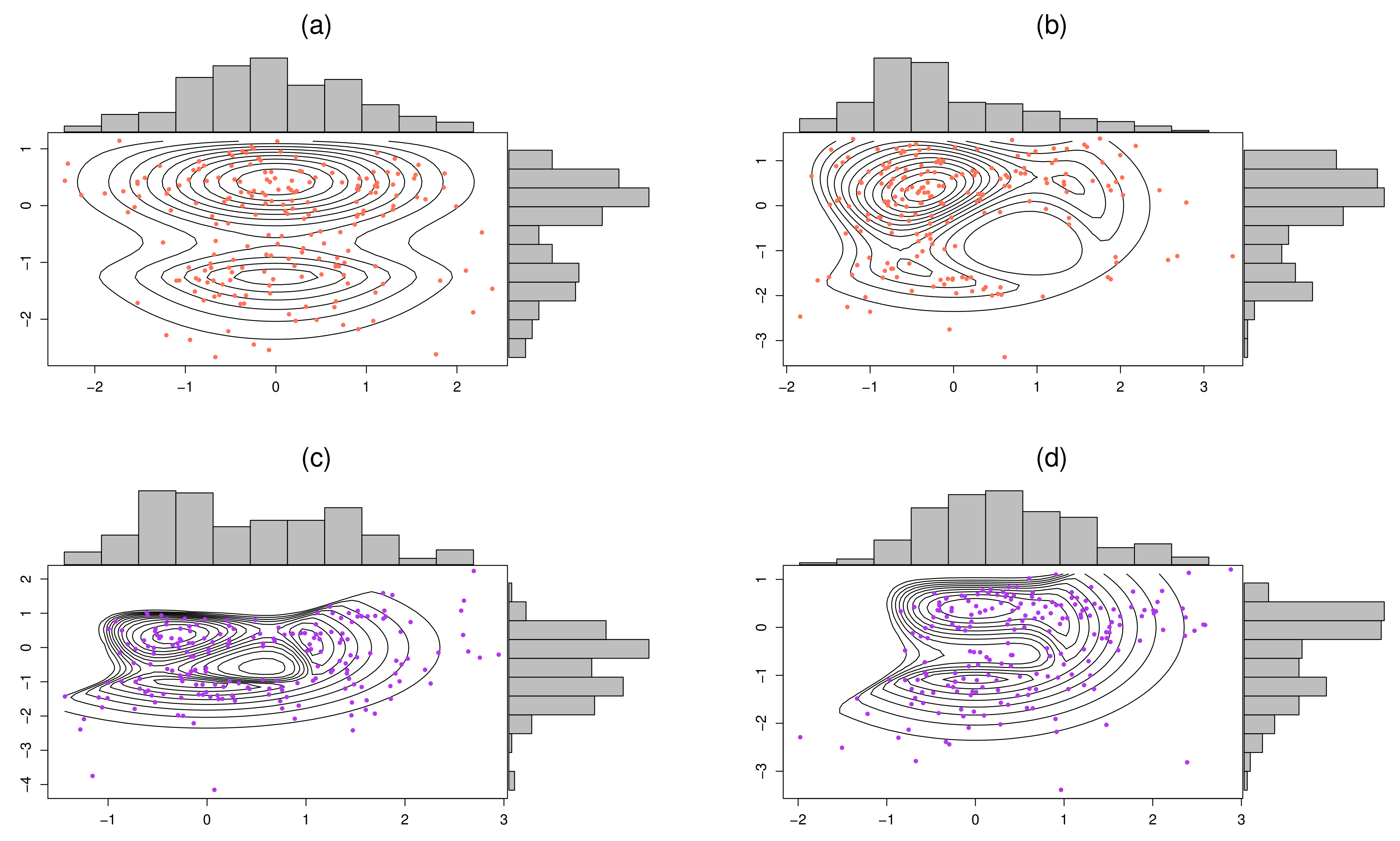
3. Examples of SSMFSSN Distributions

We present some special cases of SSMFSSN distributions which are induced by setting different mixing distributions for $\mathbf{\tau }$. For each case, additional conditional expectations are also derived for the implementation of ECME.

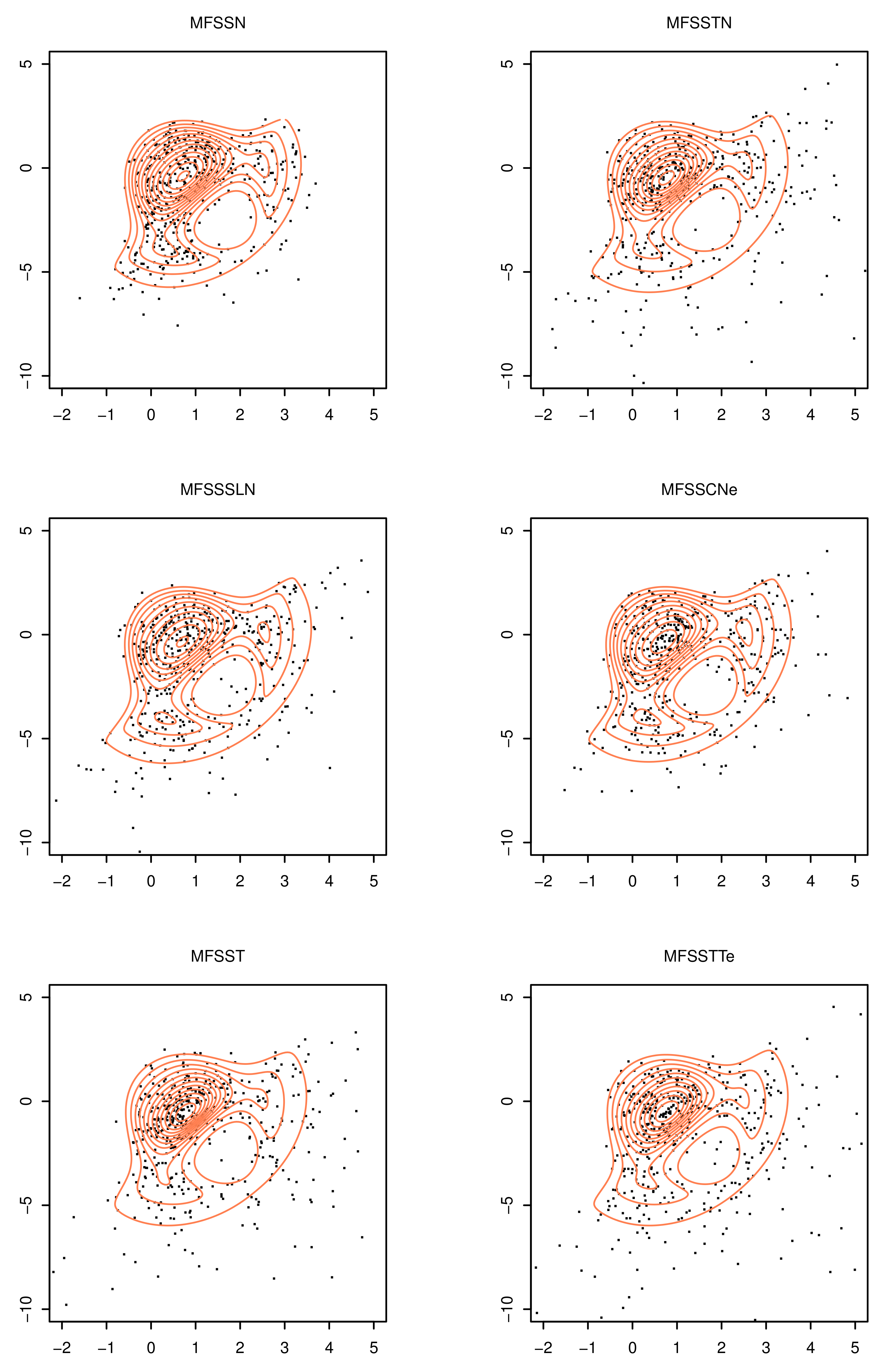
3.1. The Multivariate Flexible Skew-Symmetric-t-Normal Distribution

The multivariate flexible skew-symmetric-t-normal (MFSSTN) distribution, denoted by $\mathit{Y}$∼$MFSST{N}_p(\mathbf{\xi },\mathsf{\Sigma },\mathbf{\alpha },\nu )$, is produced by taking ${\tau }_1\sim \mathsf{\Gamma }(\nu /2,\nu /2)$ and ${\tau }_2=1$ in (10). In this case, $h_{\mathbf{\tau }}({\gamma }_1,{\gamma }_2;\mathbf{\nu })=g({\gamma }_1;\nu /2,\nu /2)$, where $g(·;\alpha ,\beta )$ represents the pdf of the gamma distribution with mean $\alpha /\beta$. The pdf of the MFSSTN distribution can be expressed as

$$f_{MFSSTN}\left(\mathit{y};\mathbf{\xi },\mathsf{\Sigma },\mathbf{\alpha },\nu \right)=2t_p\left(\mathit{y};\mathbf{\xi },\mathsf{\Sigma },\nu \right)\mathsf{\Phi }\left(\zeta \right),$$

(28)

where $t_p(·;\mathbf{\xi },\mathsf{\Sigma },\nu )$ stands for the pdf of p-dimensional multivariate t distribution with location vector $\mathbf{\xi }$, scale covariance matrix $\mathsf{\Sigma }$, and degree of freedom (DOF) equal to $\nu$. One special case of the MFSSTN distribution is the multivariate skew-t-normal (MSTN) distribution of Lin et al. [18], obtained by letting ${\mathbf{\lambda }}_j=\mathbf{0}$ for $j=2,\dots ,m$. In addition, the MFSSTN distribution reduces to MFSSN as $\nu \to \infty$.

According to (18), it is easy to observe that ${\gamma }_1|\mathit{Y}=\mathit{y}$∼$\mathsf{\Gamma }((\nu +p)/2,(\nu +{\delta }^2)/2)$, where ${\delta }^2={(\mathit{y}-\mathbf{\xi })}^{\top }{\mathsf{\Sigma }}^{-1}(\mathit{y}-\mathbf{\xi })$ denotes the squared Mahalanobis distance. Therefore,

$$E({\gamma }_1\mid \mathit{Y}=\mathit{y})=\frac{\nu +p}{\nu +{\delta }^2}\mathrm{and}E(ln{\gamma }_1\mid \mathit{Y}=\mathit{y})=\psi \left(\frac{\nu +p}{2}\right)-ln\left(\frac{\nu +{\delta }^2}{2}\right),$$

(29)

where $\psi \left(x\right)={\mathsf{\Gamma }}^{\prime }\left(x\right)/\mathsf{\Gamma }\left(x\right)$ is the digamma function.

From (20) and (21), the E-step involves the calculation of ${\widehat{s}}_{1i}^{\left(k\right)}=E({\gamma }_{1i}\mid {\mathit{y}}_i,{\widehat{\mathbf{\theta }}}^{\left(k\right)})$, ${\widehat{s}}_{2i}^{\left(k\right)}=1$, ${\widehat{s}}_{3i}^{\left(k\right)}=E(W_i\mid {\mathit{y}}_i,{\widehat{\mathbf{\theta }}}^{\left(k\right)})$ and ${\widehat{s}}_{4i}^{\left(k\right)}=E(ln{\gamma }_{1i}\mid {\mathit{y}}_i,{\widehat{\mathbf{\theta }}}^{\left(k\right)})$, which can be easily evaluated via the results of (17) and (29). As an alternative way of estimating $\nu$, the CML-Step for the MFSSTN distribution can be altered to the following CMQ-Step.

• CMQ-Step 4:${\widehat{\nu }}^{(k+1)}$ is obtained by solving the root of the following equation:

  $$1+ln\left(\frac{\nu }{2}\right)-\psi \left(\frac{\nu }{2}\right)+\frac{1}{n}\sum _{i=1}^n\left({\widehat{s}}_{4i}^{\left(k\right)}-{\widehat{s}}_{1i}^{\left(k\right)}\right)=0.$$

  (30)

3.2. The Multivariate Flexible Skew-Symmetric-Slash-Normal Distribution

Let $\mathit{Y}$ be a p-dimensional random vector with the following representation

$$\mathit{Y}=\mathbf{\xi }+{\tau }^{-1/2}{\mathsf{\Sigma }}^{1/2}\mathit{Z},$$

(31)

where $\mathit{Z}$∼$N_p(\mathbf{0},{\mathit{I}}_p)$ and is independent of $\tau \stackrel{d}{=}{U}^{1/\nu }$∼$Beta(\nu ,1)$, where U is the uniform distribution on the interval $(0,1)$. From (31), the conditional distribution $\mathit{Y}$ given $\tau$ is $N_p(\mathbf{\xi },{\tau }^{-1}\mathsf{\Sigma })$. Then, $\mathit{Y}$ has a multivariate slash distribution with pdf given by

$$\begin{array}{ccc}\hfill f_{SL}(\mathit{y};\mathbf{\xi },\mathsf{\Sigma },\nu )& =& \nu {\int }_0^1{\tau }^{\nu -1}{\varphi }_p(\mathit{y};\mathbf{\xi },{\tau }^{-1}\mathsf{\Sigma })d\tau \hfill \\ & =& \left\{\begin{array}{c}\frac{2^{\nu }\nu {\left|\mathsf{\Sigma }\right|}^{-1/2}\mathsf{\Gamma }(\nu +p/2)G({\delta }^2/2;\nu +p/2)}{{\pi }^{p/2}{\delta }^{2\nu +p}},\mathit{y}\ne \mathbf{\xi }\hfill \\ \\ \frac{\nu }{(\nu +p/2){\left(2\pi \right)}^{p/2}}{\left|\mathsf{\Sigma }\right|}^{-1/2},\mathit{y}=\mathbf{\xi }\hfill \end{array}\right.\hfill \end{array}$$

(32)

where $G(·;r)$ denotes the cdf of the gamma distribution with scale parameter 1 and shape parameter r. Using the law of iterated expectations, the mean vector and variance-covariance matrix of $\mathit{Y}$ are

$$E\left(\mathit{Y}\right)=\mathbf{\xi }\mathrm{and}\mathrm{cov}\left(\mathit{Y}\right)=\frac{\nu }{\nu -1}\mathsf{\Sigma }.$$

(33)

If we select ${\tau }_1$∼$Beta(\nu ,1)$ and ${\tau }_2=1$ for (10), this generates the multivariate flexible skew-symmetric-slash-normal (MFSSSLN) distribution, denoted by $\mathit{Y}$∼$MFSSSL{N}_p(\mathbf{\xi },\mathsf{\Sigma },\mathbf{\alpha },\nu )$, with the pdf taking the form of

$$\begin{array}{c}\hfill f_{MFSSSLN}(\mathit{y};\mathbf{\xi },\mathsf{\Sigma },\mathbf{\alpha },\nu )=2f_{SL}(\mathit{y};\mathbf{\xi },\mathsf{\Sigma },\nu )\mathsf{\Phi }\left(\zeta \right).\end{array}$$

(34)

Note that the MFSSSLN distribution contains the MFSSN distribution as a limiting case for $\nu \to \infty$ and encloses the multivariate skew-slash distribution considered by Wang and Genton [19] as a reduced case when ${\mathbf{\lambda }}_2=\cdots ={\mathbf{\lambda }}_m=\mathbf{0}$.

According to (18), the conditional distribution ${\gamma }_1\mid \mathit{y}$ is given by

$$\begin{array}{c}\hfill f({\gamma }_1\mid \mathit{y})=\left\{\begin{array}{c}\frac{{\left|\delta \right|}^{2\nu +p}{\gamma }_1^{\nu +p/2-1}exp(-{\gamma }_1{\delta }^2/2)}{2^{\nu +p/2}\mathsf{\Gamma }(\nu +p/2)G({\delta }^2/2;\nu +p/2)},\mathit{y}\ne \mathbf{\xi }\hfill \\ \\ (\nu +\frac{p}{2}){\gamma }_1^{\nu +p/2-1},\mathit{y}=\mathbf{\xi }.\hfill \end{array}\right.\end{array}$$

(35)

In addition, some algebraic manipulations yield

$$\begin{array}{c}\hfill E({\gamma }_1\mid \mathit{Y}=\mathit{y})=\left\{\begin{array}{c}\left(\frac{2\nu +p}{{\delta }^2}\right)\frac{G({\delta }^2/2;\nu +p/2+1)}{G({\delta }^2/2;\nu +p/2)},\mathit{y}\ne \mathbf{\xi }\hfill \\ \\ \frac{2\nu +p}{2\nu +p+2},\mathit{y}=\mathbf{\xi }.\hfill \end{array}\right.\end{array}$$

(36)

and

$$\begin{array}{c}\hfill E(ln{\gamma }_1\mid \mathit{Y}=\mathit{y})=\left\{\begin{array}{c}ln\left(\frac{2}{{\delta }^2}\right)+\frac{{\int }_0^{{\delta }^2/2}ln\left(x\right)x^{\nu +p/2-1}{e}^{-x}dx}{\mathsf{\Gamma }(\nu +p/2)G({\delta }^2/2;\nu +p/2)},\mathit{y}\ne \mathbf{\xi }\hfill \\ \\ \frac{-2}{2\nu +p},\mathit{y}=\mathbf{\xi }.\hfill \end{array}\right.\end{array}$$

(37)

To implement the ECME procedure for fitting MFSSSLN, the conditional expectations involved in (20) and (21) can be easily evaluated via the results of (17), (36), and (37). Besides, the DOF ${\widehat{\nu }}^{\left(k\right)}$ can be alternatively updated by maximizing the Q-function over $\nu$, leading to the following CMQ-Step:

• CMQ-Step 4:

  $${\widehat{\nu }}^{(k+1)}=-\frac{n}{{\sum }_{i=1}^n{\widehat{s}}_{4i}^{\left(k\right)}}.$$

  (38)

3.3. The Multivariate Flexible Skew-Symmetric-Contaminated-Normal Distribution

The multivariate flexible skew-symmetric-contaminated-normal (MFSSCN) distribution, denoted by $\mathit{Y}$∼$MFSSC{N}_p(\mathbf{\xi },\mathsf{\Sigma },\mathbf{\alpha },{\nu }_1,{\nu }_2)$, arises when ${\tau }_2=1$, while ${\tau }_1$ has a discrete distribution taking value ${\nu }_2\in (0,1)$ with probability ${\nu }_1$ and value 1 with probability $1-{\nu }_1$. More precisely,

$$\begin{array}{c}\hfill h({\tau }_1,\mathbf{\nu })={\nu }_1{\mathbb{I}}_{({\tau }_1={\nu }_2)}+(1-{\nu }_1){\mathbb{I}}_{({\tau }_1=1)},0<{\nu }_1<1\mathrm{and}0<{\nu }_2<1,\end{array}$$

(39)

where ${\nu }_1$ is the proportion of outliers and ${\nu }_2$ is an inflation parameter denoting the degree of contamination.

Using (14), the pdf of $\mathit{Y}$ is given by

$$\begin{array}{c}\hfill f_{MFSSCN}(\mathit{y};\mathbf{\xi },\mathsf{\Sigma },\mathbf{\zeta },{\nu }_1,{\nu }_2)=2\left\{{\nu }_1{\varphi }_p(\mathit{y};\mathbf{\xi },{\nu }_2^{-1}\mathsf{\Sigma })+(1-{\nu }_1){\varphi }_p(\mathit{y};\mathbf{\xi },\mathsf{\Sigma })\right\}\mathsf{\Phi }\left(\zeta \right).\end{array}$$

(40)

Obviously, the MFSSCN distribution reduces to the MFSSN distribution when ${\nu }_2=1$, to the multivariate skew-contaminated-normal distribution [4] when ${\mathbf{\lambda }}_2=\cdots ={\mathbf{\lambda }}_m=\mathbf{0}$, and is said to follows the “MFSSCNe" distribution if ${\nu }_1$ and ${\nu }_2$ are restricted to be equal, namely ${\nu }_1={\nu }_2=\nu$.

To obtain ${\widehat{s}}_{4i}^{\left(k\right)}$, we require the following conditional expectation

$$E({\gamma }_1\mid \mathit{Y}=\mathit{y})=\frac{1-{\nu }_1+{\nu }_1{\nu }_2^{1+p/2}exp\{(1-{\nu }_2){\delta }^2/2\}}{1-{\nu }_1+{\nu }_1{\nu }_2^{p/2}exp\{(1-{\nu }_2){\delta }^2/2\}}.$$

(41)

The resulting Q-function can be easily evaluated through (17) and (41) since ${\widehat{s}}_{2i}^{\left(k\right)}=1$. To estimate ${\nu }_1$ and ${\nu }_2$, we perform the CML-Step, so the calculation of ${\widehat{s}}_{4i}^{\left(k\right)}$ can be omitted.

3.4. The Multivariate Flexible Skew-Symmetric-t Distribution

The multivariate flexible skew-symmetric-t (MFSST) distribution, denoted by $\mathit{Y}$∼$MFSS{T}_p(\mathbf{\xi },\mathsf{\Sigma },\mathbf{\alpha },\nu )$, is created by setting ${\tau }_1={\tau }_2=\tau$ with $\tau \sim \mathsf{\Gamma }(\nu /2,\nu /2)$. Utilizing (8), the hierarchical representation for $\mathit{Y}$ can be simplified as

$$\begin{array}{c}\hfill \mathit{Y}\mid \tau \sim MFSS{N}_p(\mathbf{\xi },{\tau }_1^{-1}\mathsf{\Sigma },\mathbf{\vartheta }),\end{array}$$

(42)

where $\mathbf{\vartheta }={\left({\mathbf{\lambda }}_1^{\top },{\tau }^{-1}{\mathbf{\lambda }}_2^{\top }\cdots ,{\tau }^{-m+1}{\mathbf{\lambda }}_m^{\top }\right)}^{\top }$. Therefore, it can be verified that the MFSST distribution has the following pdf

$$f_{MFSST}\left(\mathit{y};\mathbf{\xi },\mathsf{\Sigma },\mathbf{\zeta },\nu \right)=2t_p\left(\mathit{y};\mathbf{\xi },\mathsf{\Sigma },\nu \right)T\left(\zeta \sqrt{\frac{\nu +p}{\nu +{\delta }^2}};\nu +p\right),$$

(43)

where $T(·,\nu )$ denotes the cdf of the t distribution with DOF $\nu$. The detailed proof of (43) is sketched in Appendix B. It is notable that the MFSST distribution includes the multivariate skew-t distribution of Azzalini and Capitanio [6] as a particular member by letting ${\mathbf{\lambda }}_2=\cdots ={\mathbf{\lambda }}_m=\mathbf{0}$ and the MFSSN distribution as a limiting case when $\nu$ grows to infity.

Using (18) subject to ${\gamma }_1={\gamma }_2=\gamma$, it suffices to show that

$$\begin{array}{ccc}\hfill f(\gamma \mid \mathit{y})& =& \frac{1}{T(M;\nu +p)}g\left(\gamma ;\frac{\nu +p}{2},\frac{\nu +{\delta }^2}{2}\right)\mathsf{\Phi }\left({\gamma }^{1/2}\zeta \right),\hfill \end{array}$$

(44)

where $M=\zeta \sqrt{\frac{\nu +p}{{\delta }^2+\nu }}$.

With arguments similar to those of Lin et al. [20], it is straightforward to derive

$$\begin{array}{c}\hfill E(\gamma \mid \mathit{Y}=\mathit{y})=\left(\frac{\nu +p}{{\delta }^2+\nu }\right)\frac{T\left(M\sqrt{\frac{\nu +p+2}{\nu +p}};\nu +p+2\right)}{T\left(M;\nu +p\right)}\end{array}$$

(45)

and

$$\begin{array}{ccc}\hfill E(ln\gamma \mid \mathit{Y}=\mathit{y})& =& \psi \left(\frac{\nu +p}{2}\right)-ln\left(\frac{{\delta }^2+\nu }{2}\right)\hfill \\ & & +\frac{\nu +p}{{\delta }^2+\nu }\left\{\frac{T(M\sqrt{\frac{\nu +p+2}{\nu +p}};\nu +p+2)}{T(M;\nu +p)}-1\right\}\hfill \\ & & +\frac{\zeta ({\delta }^2-1)}{\sqrt{(\nu +p){(\nu +{\delta }^2)}^3}}\frac{t(M;\nu +p)}{T(M;\nu +p)}\hfill \\ & & +\frac{1}{T(M;\nu +p)}{\int }_{-\infty }^M{\kappa }_{\nu }\left(x\right)t(x;\nu +p)dx,\hfill \end{array}$$

(46)

where

$$\begin{array}{c}\hfill {\kappa }_{\nu }\left(x\right)=\psi \left(\frac{\nu +p+1}{2}\right)-\psi \left(\frac{\nu +p}{2}\right)-ln\left(1+\frac{x^2}{\nu +p}\right)+\frac{(\nu +p)x^2-\nu -p}{(\nu +p)(\nu +p+x^2)}.\end{array}$$

Additionally, using the law of iterated expectations, we can deduce that

$$\begin{array}{ccc}\hfill E(W\gamma \mid Y=y)& =& \frac{1}{T(M;\nu +p)}\{M\sqrt{\frac{\nu +p}{{\delta }^2+\nu }}T\left(M\sqrt{\frac{\nu +p+2}{\nu +p}};\nu +p+2\right)\hfill \\ & & +{({\delta }^2+\nu )}^{-1/2}\frac{\mathsf{\Gamma }\left((\nu +p+1)/2)\right)}{\sqrt{\pi }\mathsf{\Gamma }\left((\nu +p)/2\right)}{\left(1+\frac{{\zeta }^2}{{\delta }^2+\nu }\right)}^{-\frac{\nu +p+1}{2}}\}.\hfill \end{array}$$

(47)

As a consequence, the E-step in (20) and (21) requires the calculation of ${\widehat{s}}_{1i}^{\left(k\right)}={\widehat{s}}_{2i}^{\left(k\right)}=E({\gamma }_i\mid y_i,{\mathbf{\theta }}^{\left(k\right)})$, ${\widehat{s}}_{3i}^{\left(k\right)}=E(W_i{\gamma }_i\mid y_i,{\widehat{\mathbf{\theta }}}^{\left(k\right)})$, and ${\widehat{s}}_{4i}^{\left(k\right)}=E(ln{\gamma }_i\mid y_i,{\widehat{\mathbf{\theta }}}^{\left(k\right)})$, which can be directly evaluated via (45)–(47). Moreover, the procedure of updating ${\widehat{\nu }}^{\left(k\right)}$ is the same as (30).

3.5. The Multivariate Flexible Skew-Symmetric-t-t Distribution

Consider two independent random variables ${\tau }_1$∼$\mathsf{\Gamma }({\nu }_1/2,{\nu }_1/2)$ and ${\tau }_2$∼$\mathsf{\Gamma }({\nu }_2/2,{\nu }_2/2)$ with joint pdf given by

$$\begin{array}{c}\hfill h_{\mathbf{\tau }}({\gamma }_1,{\gamma }_2;{\nu }_1,{\nu }_2)=g({\gamma }_1;{\nu }_1/2,{\nu }_1/2)g({\gamma }_2;{\nu }_2/2,{\nu }_2/2).\end{array}$$

(48)

Using (14), we thus generate the multivariate flexible skew-symmetric-t-t (MFSSTT) distribution, denoted by $\mathit{Y}$∼$MFSST{T}_p(\mathbf{\xi },\mathsf{\Sigma },\mathbf{\alpha },{\nu }_1,{\nu }_2)$, whose pdf is of the form

$$f_{MFSSTT}\left(\mathit{y};\mathbf{\xi },\mathsf{\Sigma },\mathbf{\alpha },\mathbf{\nu }\right)=2t_p(\mathit{y};\mathbf{\xi },\mathsf{\Sigma },{\nu }_1)T(\zeta ;{\nu }_2).$$

(49)

When the two DOFs are restricted to be equal, namely ${\nu }_1={\nu }_2=\nu$, $\mathit{Y}$ is said to follow the ‘MFSSTTe’ distribution. One thing worth noting is that the MFSSTT distribution reduces to the MFSSN distribution when $({\nu }_1,{\nu }_2)\to (\infty ,\infty )$, to the MFSSTN distribution by letting ${\nu }_1=\nu$ and ${\nu }_2=\infty$, and embeds the multivariate skew-t-t (MSTT) distribution introduced by Wang et al. [21] as a special case under the setting of ${\mathbf{\lambda }}_2=\cdots ={\mathbf{\lambda }}_m=\mathbf{0}$.

According to (18), it is easy to see ${\gamma }_1\mid \mathit{Y}=\mathit{y}$∼$\mathsf{\Gamma }\left(({\nu }_1+p)/2,({\nu }_1+{\delta }^2)/2\right)$. The conditional pdf of ${\gamma }_2$ given $\mathit{Y}=\mathit{y}$ is

$$\begin{array}{c}\hfill f({\gamma }_2\mid \mathit{y})=\frac{g\left({\gamma }_2;{\nu }_2/2,{\nu }_2/2\right)\mathsf{\Phi }\left({\gamma }_2^{1/2}\zeta \right)}{T(\zeta ;{\nu }_2)}.\end{array}$$

(50)

Further, we have the following conditional expectations:

$$\begin{array}{c}\hfill E({\gamma }_2\mid \mathit{Y}=\mathit{y})=\frac{T\left(\zeta \sqrt{\frac{{\nu }_2+2}{{\nu }_2}};{\nu }_2+2\right)}{T(\zeta ;{\nu }_2)}\end{array}$$

(51)

and

$$\begin{array}{ccc}\hfill E(ln{\gamma }_2\mid \mathit{Y}=\mathit{y})& =& \psi \left(\frac{{\nu }_2+1}{2}\right)-ln\left(\frac{{\nu }_2}{2}\right)+\frac{T\left(\zeta \sqrt{\frac{{\nu }_2+2}{{\nu }_2}};{\nu }_2+2\right)}{T(\zeta ;{\nu }_2)}-1\hfill \\ & & -\left(\frac{\zeta }{{\nu }_2}\right)\frac{t(\zeta ;{\nu }_2)}{T(\zeta ;{\nu }_2)}-\frac{1}{T(\zeta ;{\nu }_2)}{\int }_{-\infty }^{\zeta }ln\left(1+\frac{x^2}{{\nu }_2}\right)t(x;{\nu }_2)dx.\hfill \end{array}$$

(52)

Applying the law of iterated expectations to (15) and (50) gives

$$\begin{array}{c}\hfill E(W{\gamma }_2\mid \mathit{Y}=\mathit{y})=\frac{1}{T(\zeta ;{\nu }_2)}\left\{\zeta T\left(\zeta \sqrt{\frac{{\nu }_2+2}{{\nu }_2}};{\nu }_2+2\right)+t(\zeta ;{\nu }_2)\right\}.\end{array}$$

(53)

With slight modifications as defined in (20) and (21), the necessary conditional expectations in the E-step include ${\widehat{s}}_{1i}^{\left(k\right)}=E({\gamma }_{1i}\mid {\mathit{y}}_i,{\widehat{\mathbf{\theta }}}^{\left(k\right)})$, ${\widehat{s}}_{2i}^{\left(k\right)}=E({\gamma }_{2i}\mid {\mathit{y}}_i,{\widehat{\mathbf{\theta }}}^{\left(k\right)})$, ${\widehat{s}}_{3i}^{\left(k\right)}=E(W_i{\gamma }_{2i}\mid {\mathit{y}}_i,{\widehat{\mathbf{\theta }}}^{\left(k\right)})$, ${\widehat{s}}_{4i}^{\left(k\right)}=E(ln{\gamma }_{1i}\mid {\mathit{y}}_i,{\widehat{\mathbf{\theta }}}^{\left(k\right)})$, and ${\widehat{s}}_{5i}^{\left(k\right)}=E(ln{\gamma }_{2i}\mid {\mathit{y}}_i,{\widehat{\mathbf{\theta }}}^{\left(k\right)})$, which can be easily evaluated via the results given in (29) and (51)–(53), respectively. To numerically estimate ${\nu }_1$ and ${\nu }_2$ for the MFSSTT distribution, we resort to the following two root-finding equations:

• CMQ-Step 4:${\widehat{\nu }}_1^{(k+1)}$ and ${\widehat{\nu }}_2^{(k+1)}$ are obtained by solving the roots of the following two equations:

  $$1+ln\left(\frac{{\nu }_1}{2}\right)-\psi \left(\frac{{\nu }_1}{2}\right)+\frac{1}{n}\sum _{i=1}^n\left({\widehat{s}}_{4i}^{\left(k\right)}-{\widehat{s}}_{1i}^{\left(k\right)}\right)=0$$

  (54)

  and

  $$1+ln\left(\frac{{\nu }_2}{2}\right)-\psi \left(\frac{{\nu }_2}{2}\right)+\frac{1}{n}\sum _{i=1}^n\left({\widehat{s}}_{5i}^{\left(k\right)}-{\widehat{s}}_{2i}^{\left(k\right)}\right)=0.$$

  (55)

4. Simulation Studies

4.1. Recovery of the True Underlying Parameters

The first experiment intends to investigate the ability of the proposed ECME algorithm to recover the true underlying parameters. Monte Carlo samples of different sample sizes $n=100$, 250, 500, and 1000 were generated from the MFSSN distributions specified in (7) and five examples of SSMFSSN distributions studied in Section 3. For ease of exposition, we considered the Hadamard power transformation of order three ($K=3$) that allows two shape parameters in the skewing function $\mathsf{\Phi }(·)$. Moreover, the flatness parameters for MFSSCN and MFSSTT were assumed to be equal, say ${\nu }_1={\nu }_2=\nu$, referred to as the MFSSCNe and MFSSTTe distributions. The presumed true parameters were $\mathbf{\xi }={(1,-1)}^{\top }$, $\mathbf{\sigma }=\mathrm{vech}\left(\mathsf{\Sigma }\right)={(1,0.5,4)}^{\top }$, ${\mathbf{\lambda }}_1={(-2,2)}^{\top }$, and ${\mathbf{\lambda }}_2={(1,-1)}^{\top }$. Furthermore, $\nu =3$ was taken for the MFSSTN, MFSSSLN, MFSST, and MFSSTTe distributions, while $\nu =0.7$ was adopted for the MFSSCNe distribution since its support lies within the interval $(0,1)$. As an illustration, Figure 2 displays the scatter plots superimposed on the fitted contours for each type of data simulated from one trail.

For all scenarios, the accuracies of the parameter estimates are assessed by computing the mean absolute bias (MAB) and the root mean square error (RMSE) over $R=100$ replications. For a vector of parameters $\mathbf{\theta }={({\theta }_1,\dots ,{\theta }_p)}^{\top }$, these measures are, respectively, defined as

$$\mathrm{MAB}=\frac{1}{pR}\sum _{k=1}^p\sum _{r=1}^R|{\widehat{\theta }}_{kr}-{\theta }_k^A|\mathrm{and}\mathrm{RMSE}=\sqrt{\frac{1}{pR}{\displaystyle \sum _{k=1}^p}{\displaystyle \sum _{r=1}^R}{({\widehat{\theta }}_{kr}-{\theta }_k^A)}^2},$$

(56)

where ${\widehat{\theta }}_{kr}$ denotes the ML estimate of the kth parameter at the rth replication and ${\theta }_k^A$ represents the actual value of ${\theta }_k$.

The experimental results are summarized in

Table 1. Simulation results based on 100 replications with different sample sizes.

Model	Parameter	n = 100		n = 250		n = 500		n = 1000
		MAB	RMSE	MAB	RMSE	MAB	RMSE	MAB	RMSE
MFSSN	$\mathbf{\xi }$	0.090	0.122	0.057	0.074	0.037	0.048	0.027	0.033
	$\mathbf{\sigma }$	0.257	0.382	0.143	0.209	0.115	0.168	0.081	0.123
	${\mathbf{\lambda }}_1$	0.476	0.625	0.203	0.270	0.111	0.155	0.079	0.112
	${\mathbf{\lambda }}_2$	0.339	0.489	0.160	0.209	0.104	0.131	0.064	0.082
MFSSTN	$\mathbf{\xi }$	0.095	0.127	0.062	0.086	0.040	0.053	0.028	0.036
	$\mathbf{\sigma }$	0.419	0.673	0.244	0.383	0.158	0.241	0.121	0.179
	${\mathbf{\lambda }}_1$	0.382	0.469	0.349	0.426	0.317	0.382	0.306	0.355
	${\mathbf{\lambda }}_2$	0.335	0.439	0.194	0.244	0.177	0.216	0.151	0.181
	$\nu$	2.495	10.745	0.458	0.651	0.319	0.413	0.203	0.258
MFSSSLN	$\mathbf{\xi }$	0.091	0.121	0.052	0.069	0.036	0.047	0.025	0.035
	$\mathbf{\sigma }$	0.424	0.641	0.306	0.489	0.190	0.314	0.127	0.200
	${\mathbf{\lambda }}_1$	0.458	0.588	0.267	0.347	0.216	0.269	0.174	0.206
	${\mathbf{\lambda }}_2$	0.470	0.614	0.259	0.378	0.174	0.227	0.114	0.138
	$\nu$	6.530	11.849	3.425	8.206	1.191	3.251	0.481	0.721
MFSSCNe	$\mathbf{\xi }$	0.087	0.117	0.048	0.064	0.036	0.047	0.026	0.034
	$\mathbf{\sigma }$	0.363	0.546	0.285	0.440	0.223	0.339	0.133	0.202
	${\mathbf{\lambda }}_1$	0.446	0.595	0.288	0.353	0.202	0.247	0.138	0.174
	${\mathbf{\lambda }}_2$	0.426	0.586	0.265	0.347	0.178	0.219	0.131	0.160
	$\nu$	0.199	0.216	0.162	0.176	0.116	0.137	0.083	0.098
MFSST	$\mathbf{\xi }$	0.114	0.152	0.069	0.091	0.042	0.055	0.032	0.040
	$\mathbf{\sigma }$	0.393	0.586	0.250	0.386	0.160	0.238	0.132	0.216
	${\mathbf{\lambda }}_1$	0.453	0.559	0.265	0.329	0.207	0.253	0.194	0.228
	${\mathbf{\lambda }}_2$	0.355	0.468	0.215	0.273	0.137	0.175	0.110	0.139
	$\nu$	1.152	2.210	0.430	0.621	0.266	0.366	0.207	0.265
MFSSTTe	$\mathbf{\xi }$	0.114	0.146	0.070	0.094	0.047	0.061	0.029	0.038
	$\mathbf{\sigma }$	0.400	0.654	0.213	0.323	0.165	0.255	0.115	0.188
	${\mathbf{\lambda }}_1$	0.437	0.546	0.411	0.476	0.406	0.453	0.414	0.438
	${\mathbf{\lambda }}_2$	0.313	0.409	0.216	0.260	0.183	0.217	0.167	0.193
	$\nu$	1.332	2.733	0.424	0.573	0.300	0.408	0.210	0.279

. It is readily seen both MAB and RMSE values tend to approach zero with increasing the sample size. While this study is limited to the simplest case $(p=2;m=2)$, our developed ECME algorithm shows favorable ability to recover the true parameter values with data generated exactly according to model assumptions. Similar experiments have also been undertaken on more complex scenarios $(p=3;m=3)$. The extensive results would not necessarily be excessively reported since the conclusions are in accordance with those already presented.

4.2. Comparing the Proposed Procedure with Convolution-Type EM Algorithms

The second experiment aims to compare the performance of the proposed selection-type ECME procedure outlined in Section 2.2 with the traditional EM-based algorithms derived based on convolution-type representations. As an illustration, we consider the fitting of MSN, MST, and MSCN distributions arisen from the multivariate skew-normal independent (SNI) family studied by Cabral et al. [22]. As discussed above, they are special cases of our proposed MFSSN, MFSST, and MFSSCN distributions by setting ${\mathbf{\lambda }}_2=\cdots ={\mathbf{\lambda }}_m=\mathbf{0}$. Accordingly, the CMQ-Step 1 in Section 2 can be simplified as follows:

• CMQ-Step 1: Fixing $\mathsf{\Sigma }={\widehat{\mathsf{\Sigma }}}^{\left(k\right)}$ and ${\mathbf{\lambda }}_1={\widehat{\mathbf{\lambda }}}_1^{\left(k\right)}$, we obtain ${\widehat{\mathbf{\xi }}}^{(k+1)}$ by

  $$\begin{array}{ccc}\hfill {\widehat{\mathbf{\xi }}}^{(k+1)}& =& {\left[{\mathit{I}}_p\sum _{i=1}^n{\widehat{s}}_{1i}^{\left(k\right)}+{\widehat{\mathsf{\Sigma }}}^{\left(k\right)}{\hat{\Delta }}_1^{\top \left(k\right)}{\mathbf{1}}_p{\mathbf{1}}_p^{\top }{\hat{\Delta }}_1^{\left(k\right)}\sum _{i=1}^n{\widehat{s}}_{2i}^{\left(k\right)}\right]}^{-1}\{\sum _{i=1}^n{\widehat{s}}_{1i}^{\left(k\right)}{\mathit{y}}_i\hfill \\ & & +{\widehat{\mathsf{\Sigma }}}^{\left(k\right)}{\hat{\Delta }}_1^{\top \left(k\right)}{\mathbf{1}}_p{\mathbf{1}}_p^{\top }{\hat{\Delta }}_1^{\left(k\right)}\sum _{i=1}^n{\widehat{s}}_{2i}^{\left(k\right)}{\mathit{y}}_i-{\widehat{\mathsf{\Sigma }}}^{\left(k\right)}{\hat{\Delta }}_1^{\top \left(k\right)}{\mathbf{1}}_p\sum _{i=1}^n{\widehat{s}}_{3i}^{\left(k\right)}\}.\hfill \end{array}$$

  (57)

In total, 100 Monte Carlo (MC) samples of sizes $n=100$, 500, and 1000 were generated from each of the three distributions. The true parameters were the same as those given in the previous experiment except for ${\mathbf{\lambda }}_2=\mathbf{0}$. Each simulated sample was fitted twice with the proposed selection-type ECME procedure and the EM-type algorithm based on convolution-type representations, as implemented by the mixsmsn R package [23]. For a fair comparison, we started the two algorithms using the same initial values as described at the end of Section 2. All computations were carried out by Microsoft R package 3.5.1 in win64 environment of a desktop computer with 2.80-GHz/Intel Core(TM) i7-7700HQ CPU Processor and 16.0 GB RAM. Performance evaluation was assessed by the execution CPU time and the converged log-likelihood maxima.

The box plots depicted in Figure 3 reveal the selection-type algorithm demands much lower computational cost than those required for the convolution-type algorithm. The phenomenon is more apparent for the MST and MSCN distributions, particularly for larger n. The high efficiency of the selection-type algorithm can be ascribed to the fact that its E-step is designed by virtue of simplification. Finally, it is worth mentioning that both algorithms can achieve the same final log-likelihood, as demonstrated by violin plots in Figure 4.   

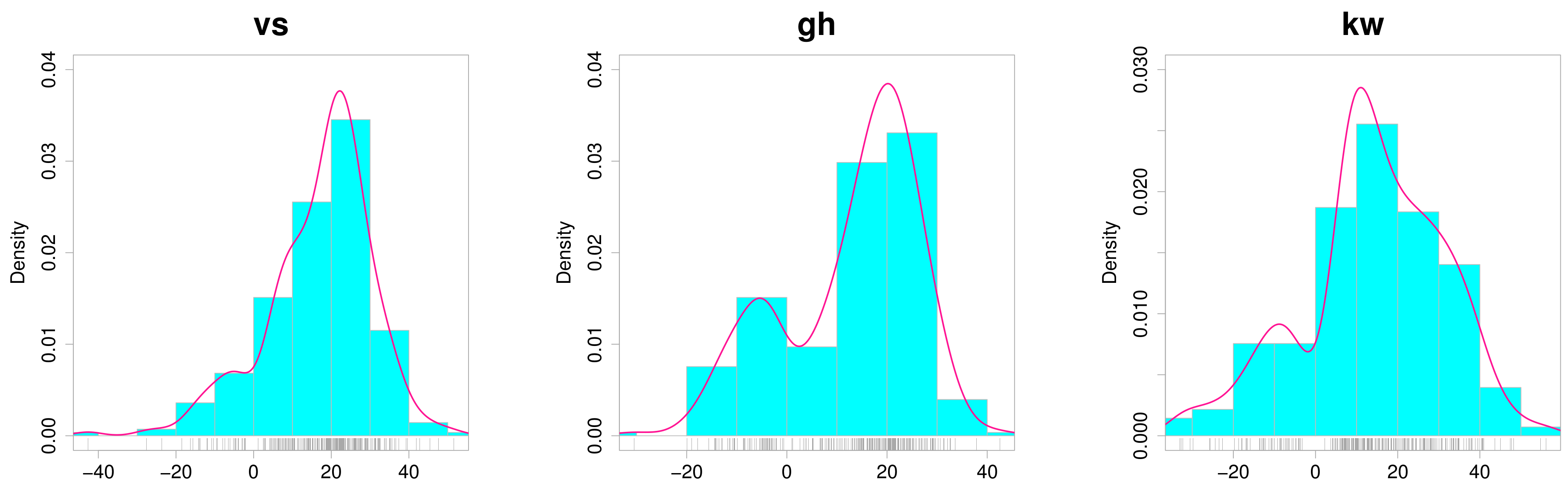
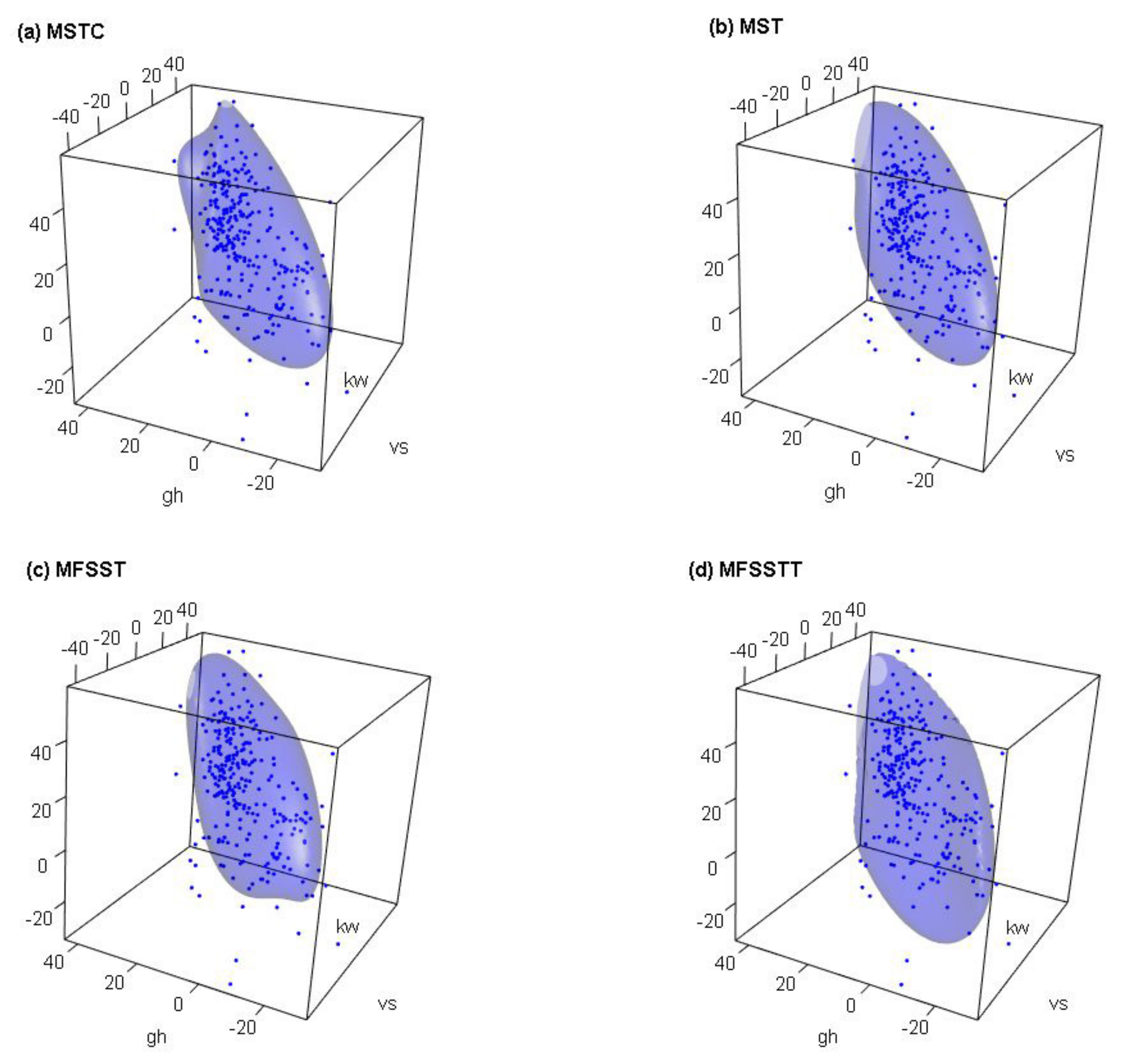
5. An Illustrative Example: The Wind Speed Data

We considered a trivariate dataset analyzed by Azzalini and Genton [24] for the study of spatial distribution of wind speed by means of the MST and various MSSMSN distributions proposed by Azzalini and Capitanio [6] and Arellano-Valle et al. [5], respectively. This dataset contains 278 hourly average speed assembled at three meteorological towers: Goodnoe Hills (gh), Kennewick (kw), and Vansycle (vs) from 23 February to 30 November 2003 recorded at midnight when wind speeds tend to peak. The positive and negative signs of wind speed measurements represent a westerly wind direction and an easterly wind direction, respectively. The Ljung–Box test indicates weak serial correlation for observations measured at the three stations. For modeling these data, we followed Azzalini and Genton [24] to treat the observations as being independent and identically distributed. Figure 5 presents histograms overlaid with kernel density curves obtained by using R density() function for measurements collected at each tower.

Six SSMFSSN models of order 3 were considered to fit the wind speed data. For the sake of comparison, the MST, MSTN, and MSTC distributions belonging to the MSSMSN family [5] were also fitted as sub-models of SSMFSSN subject to the constraint of ${\mathbf{\lambda }}_2=\mathbf{0}$. To select an appropriate model from the candidates, we adopted the Akaike information criterion (AIC) [25] and the Bayesian information criterion (BIC) [26], which are the two most widely used model selection indices based on penalized likelihood and applicable for both nested and non-nested models. The two criteria are defined as

$$\mathrm{AIC}=2d-2{\ell }_{max}\mathrm{and}\mathrm{BIC}=dlogn-2{\ell }_{max},$$

(58)

where d is the number of free parameters in the model and ${\ell }_{\max }$ is the maximized log-likelihood value. A lower AIC or BIC value indicates that a closer fit of the model to the data.

Table 2. Summary results from fitting various models to the wind speed data. The model with the smallest value of AIC and BIC is displayed in bold.

Family	Model	${\mathit{\ell }}_{max}$	d	AIC	BIC
	MSTC	–3178.7	13	6383.4	6430.5
MSSMSN	MST	–3180.7	13	6387.5	6434.6
	MSTN	–3180.9	13	6387.8	6434.9
	MFSSN	–3171.7	15	6373.4	6427.8
	MFSSTN	–3145.6	16	6323.1	6381.2
SSMFSSN	MFSSSLN	–3147.1	16	6326.2	6384.2
	MFSSCN	–3145.6	16	6323.3	6381.3
	MFSST	–3143.0	16	6318.1	6376.1
	MFSSTT	–3138.2	17	6310.4	6372.1

compares the ML estimation results for nine candidate models. As can be seen, our proposed SSMFSSN models perform favorably as compared to three MSSMSN analogs because they suffer from a lack of ability to capture the possibly bimodal behavior of the wind speed data (Figure 5). Accordingly, the MFSSTT distribution provides the best fit in terms of the lowest value of AIC as well as BIC, followed by the MFSST distribution. The MSTC and MST are the top two MSSMSN models with smaller AIC and BIC values.

Table 3. ML estimates of key parameters for six SSMFSSN models. The associated standard errors are shown in parentheses.

Parameter	MFSSN	MFSSTN	MFSSSLN	MFSSCN	MFSST	MFSSTT
${\xi }_1$	23.0(0.05)	21.3 (0.09)	21.1 (0.04)	21.5 (0.07)	19.9 (0.06)	18.6 (0.08)
${\xi }_2$	14.8 (0.04)	15.6 (0.08)	15.2 (0.04)	15.0 (0.07)	15.1 (0.04)	15.0 (0.06)
${\xi }_3$	14.6 (0.04)	14.9 (0.06)	14.8 (0.02)	15.4 (0.04)	13.4 (0.08)	12.6 (0.09)
${\sigma }_{11}$	221.2 (0.26)	122.9 (0.49)	80.6 (0.24)	115.8 (0.31)	115.6 (0.21)	115.6 (0.25)
${\sigma }_{21}$	138.8 (0.16)	96.4 (0.36)	64.6 (0.18)	91.5 (0.24)	92.8 (0.15)	93.2 (0.17)
${\sigma }_{31}$	151.0 (0.13)	104.8 (0.26)	69.5 (0.13)	99.1 (0.16)	102.9 (0.18)	106.0 (0.19)
${\sigma }_{22}$	181.3 (0.10)	134.5 (0.27)	90.3 (0.16)	128.0 (0.18)	131.2 (0.18)	132.1 (0.20)
${\sigma }_{32}$	111.4 (0.07)	80.8 (0.18)	54.4 (0.09)	79.6 (0.12)	78.8 (0.15)	79.1 (0.15)
${\sigma }_{33}$	296.4 (0.07)	203.4 (0.19)	134.0 (0.13)	187.2 (0.09)	204.4 (0.24)	206.7 (0.27)
${\lambda }_{11}$	–1.7 (0.01)	–0.4 (0.04)	–0.2 (0.01)	–0.3 (0.02)	0.1 (0.02)	1.0 (0.02)
${\lambda }_{12}$	1.6 (0.04)	1.1 (0.04)	1.0 (0.03)	1.3 (0.04)	1.3 (0.01)	3.2 (0.01)
${\lambda }_{13}$	1.9 (0.04)	1.4 (0.04)	1.1 (0.02)	1.3 (0.02)	1.4 (0.01)	2.8 (0.02)
${\lambda }_{21}$	–0.7 (1.99)	–0.1 (2.36)	0.0 (1.03)	–0.1 (1.53)	–0.2 (0.04)	1.2 (0.32)
${\lambda }_{22}$	–0.7 (0.05)	–0.4 (0.25)	–0.2 (0.05)	–0.4 (0.19)	–0.5 (0.01)	–1.6 (0.21)
${\lambda }_{23}$	–0.1 (1.52)	–0.2 (1.98)	–0.1 (0.78)	–0.2 (1.18)	–0.1 (0.02)	–2.3 (0.17)
${\nu }_1$	–	5.0 (0.18)	1.5 (0.03)	0.2 (0.04)	4.7 (0.06)	4.7 (0.08)
${\nu }_2$	–	–	–	0.2 (0.54)	–	1.0 (0.16)

summarizes the resulting ML estimates of 6 considered SSMFFSN models together with their asymptotic standard errors obtained by performing the parametric bootstrap method [27]. Notably, the estimates of the shape and flat parameters indicate the presence of skewed and leptokurtic characteristics toward different directions among the three variables. As an illustration, the fitted 3D contour densities of MSTC, MST, MFSST, and MFSSTT distributions are depicted in Figure 6. It is interesting to see that the MFSSTT model having the smallest AIC and BIC can adapt the shape of the wind speed data more closely than the other three competitors.

6. Conclusions

We introduce a novel family of SSMFSSN distributions as a generalization of the work of Mahdavi et al. [10] that can capture simultaneously the dependency among multivariate responses, skewness, heavy-tailedness, and, in particular, multimodal density shapes without resorting to the use of finite mixtures [14,15,21]. Since the SSMFSSN model cannot be represented by a convolution-type form, this stimulates us to devise a feasible ECME algorithm for ML estimation under the selection-type mechanism. The effectiveness and efficiency of the algorithm are evaluated by conducting two simulation studies. Numerical analysis of a real dataset highlights the potential and capability of our proposed approach as a promising alternative tool for modeling multimodal multivariate data with asymmetrical behavior. Computer programs for implementation of our methods can be installed as a R package from Github devtools::install_github(“a-mahdavi/SSMFSSN.EM”). Further developments of the current approach could be exploited for powerful extensions of the factor analysis model or finite mixtures thereof with censored or possibly missing values that were considered recently by the authors of [28,29,30,31,32,33,34,35]. One limitation of the SSMFSSN model is that it may not be suited to the data with modes having too far distances. Another worthwhile extension of this work is to pursue a mixture modeling framework of the current approach that would be an effective way to resolve this problem.

References

1. Branco, M.D.; Dey, D.K. A general class of multivariate skew-elliptical distributions. J. Multivar. Anal. 2001, 79, 99–113. [Google Scholar] [CrossRef] [Green Version]
2. Azzalini, A.; Valle, A.D. The multivariate skew-normal distribution. Biometrika 1996, 83, 715–726. [Google Scholar] [CrossRef]
3. Arellano-Valle, R.B.; Genton, M.G. On fundamental skew distributions. J. Multivar. Anal. 2005, 96, 93–116. [Google Scholar] [CrossRef] [Green Version]
4. Ferreira, C.S.; Lachos, V.H.; Bolfarine, H. Likelihood-based inference for multivariate skew scale mixtures of normal distributions. AStA Adv. Stat. Anal. 2016, 100, 421–441. [Google Scholar] [CrossRef]
5. Arellano-Valle, R.B.; Ferreira, C.S.; Genton, M.G. Scale and shape mixtures of multivariate skew-normal distributions. J. Multivar. Anal. 2018, 166, 98–110. [Google Scholar] [CrossRef] [Green Version]
6. Azzalini, A.; Capitanio, A. Distributions generated by perturbation of symmetry with emphasis on a multivariate skew t-distribution. J. R. Stat. Soc. Ser. B 2003, 65, 367–389. [Google Scholar] [CrossRef]
7. Wang, J.; Boyer, J.; Genton, M.G. A skew-symmetric representation of multivariate distributions. Stat. Sin. 2004, 1259–1270. Available online: https://0-www-jstor-org.brum.beds.ac.uk/stable/24307231 (accessed on 5 January 2005).
8. Ma, Y.; Genton, M.G. Flexible class of skew-symmetric distributions. Scand. J. Stat. 2004, 31, 459–468. [Google Scholar] [CrossRef] [Green Version]
9. Styan, G.P. Hadamard products and multivariate statistical analysis. Linear Algebra Its Appl. 1973, 6, 217–240. [Google Scholar] [CrossRef] [Green Version]
10. Mahdavi, A.; Amirzadeh, V.; Jamalizadeh, A.; Lin, T.I. Maximum likelihood estimation for scale-shape mixtures of flexible generalized skew normal distributions via selection representation. Comput. Stat. 2021, 36, 2201–2230. [Google Scholar] [CrossRef]
11. Dempster, A.P.; Laird, N.M.; Rubin, D.B. Maximum likelihood from incomplete data via the EM algorithm. J. R. Stat. Soc. Ser. B 1977, 39, 1–22. [Google Scholar]
12. Meng, X.L.; Rubin, D.B. Maximum likelihood estimation via the ECM algorithm: A general framework. Biometrika 1993, 80, 267–278. [Google Scholar] [CrossRef]
13. Liu, C.; Rubin, D.B. The ECME algorithm: A simple extension of EM and ECM with faster monotone convergence. Biometrika 1994, 81, 633–648. [Google Scholar] [CrossRef]
14. Lin, T.I. Maximum likelihood estimation for multivariate skew normal mixture models. J. Multivar. Anal. 2009, 100, 257–265. [Google Scholar] [CrossRef] [Green Version]
15. Lin, T.I. Robust mixture modeling using multivariate skew t distributions. Stat. Comp. 2010, 20, 343–356. [Google Scholar] [CrossRef]
16. Lin, T.I.; Lee, J.C.; Yen, S.Y. Finite mixture modelling using the skew normal distribution. Stat. Sin. 2007, 909–927. Available online: https://0-www-jstor-org.brum.beds.ac.uk/stable/24307705 (accessed on 5 December 2007).
17. R Development Core Team. R: A Language and Environment for Statistical Computing; R Foundation for Statistical Computing: Vienna, Austria, 2020; Available online: http://www.R-project.org (accessed on 10 January 2021).
18. Lin, T.I.; Ho, H.J.; Lee, C.-R. Flexible mixture modelling using the multivariate skew-t-normal distribution. Stat. Comp. 2014, 24, 531–546. [Google Scholar] [CrossRef]
19. Wang, J.; Genton, M.G. The multivariate skew-slash distribution. J. Stat. Plan. Inference 2006, 136, 209–220. [Google Scholar] [CrossRef]
20. Lin, T.I.; Lee, J.C.; Hsieh, W.J. Robust mixture modeling using the skew t distribution. Stat. Comp. 2007, 17, 81–92. [Google Scholar] [CrossRef]
21. Wang, W.L.; Jamalizadeh, A.; Lin, T.I. Finite mixtures of multivariate scale-shape mixtures of skew-normal distributions. Stat. Pap. 2020, 61, 2643–2670. [Google Scholar] [CrossRef]
22. Cabral, C.R.B.; Lachos, V.H.; Prates, M.O. Multivariate mixture modeling using skew-normal independent distributions. Comput. Stat. Data. Anal. 2012, 56, 126–142. [Google Scholar] [CrossRef]
23. Prates, M.O.; Lachos, V.H.; Cabral, C.R.B. mixsmsn: Fitting finite mixture of scale mixture of skew-normal distributions. J. Stat. Softw. 2013, 54, 1–20. [Google Scholar] [CrossRef] [Green Version]
24. Azzalini, A.; Genton, M.G. Robust likelihood methods based on the skew-t and related distributions. Int. Stat. Rev. 2008, 76, 106–129. [Google Scholar] [CrossRef]
25. Akaike, H. A new look at the statistical model identification. IEEE. Trans. Autom. Control 1974, 19, 716–723. [Google Scholar] [CrossRef]
26. Schwarz, G. Estimating the dimension of a model. Ann. Stat. 1978, 6, 461–464. [Google Scholar] [CrossRef]
27. Efron, B.; Tibshirani, R. Bootstrap methods for standard errors, confidence intervals, and other measures of statistical accuracy. Stat. Sci. 1986, 54–75. Available online: https://0-www-jstor-org.brum.beds.ac.uk/stable/2245500 (accessed on 22 May 2003). [CrossRef]
28. Lin, T.I.; Wu, P.H.; McLachlan, G.J.; Lee, S.X. A robust factor analysis model using the restricted skew-t distribution. Test 2015, 24, 510–531. [Google Scholar] [CrossRef]
29. Liu, M.; Lin, T. Skew-normal factor analysis models with incomplete data. J. Appl. Stat. 2015, 42, 789–805. [Google Scholar] [CrossRef]
30. Wang, W.L.; Liu, M.; Lin, T.I. Robust skew-t factor analysis models for handling missing data. Stat. Methods. Appl. 2017, 26, 649–672. [Google Scholar] [CrossRef]
31. Lin, T.I.; Wang, W.L.; McLachlan, G.J.; Lee, S.X. Robust mixtures of factor analysis models using the restricted multivariate skew-t distribution. Stat. Model. 2018, 28, 50–72. [Google Scholar] [CrossRef] [Green Version]
32. Wang, W.L.; Castro, L.M.; Lachos, V.H.; Lin, T.I. Model-based clustering of censored data via mixtures of factor analyzers. Comput. Stat. Data. Anal. 2019, 140, 104–121. [Google Scholar] [CrossRef]
33. Wang, W.L.; Castro, L.M.; Hsieh, W.C.; Lin, T.I. Mixtures of factor analyzers with covariates formodeling multiply censored dependent variables. Stat. Pap. 2021. [Google Scholar]
34. Wang, W.L.; Lin, T.I. Robust clustering of multiply censored data via mixtures of t factor analyzers. TEST 2021. [Google Scholar] [CrossRef]
35. Wang, W.L.; Lin, T.I. Robust clustering via mixtures of t factor analyzers with incomplete data. Adv. Data Anal. Classif. 2021. [Google Scholar] [CrossRef]
Figure 1. Four scatter-contour plots coupled with their marginal histograms of the bivariate MFSSN distribution: (a) m = 2 , λ 1 = ( 0 , 2 ) and λ 2 = ( 0 , 2 ) (bimodal); (b) m = 2 , λ 1 = ( 2 , 2 ) and λ 2 = ( 1 , 1 ) (trimodal); (c) m = 3 , λ 1 = ( 2 , 2 ) , λ 2 = ( 1 , 1 ) and λ 3 = ( 2 , 2 ) (trimodal); (d) m = 3 , λ 1 = ( 0 , 2 ) , λ 2 = ( 0 , 2 ) and λ 3 = ( 2 , 1 ) (trimodal).
Symmetry 13 01343 g001
Figure 2. Scatter-contour plots of one simulation case with 500 random samples generated from six subfamilies of the proposed model.
Symmetry 13 01343 g002
Figure 3. Box plots of CPU time for convergence of selection-type and convolution-type algorithms for fitting MSN, MST, and MSCN distributions under various sample sizes.
Symmetry 13 01343 g003
Figure 4. Violin plots of converged log-likelihood obtained by selection and convolution EM-type algorithms for fitting MSN, MST, and MSCN distributions under various sample sizes.
Symmetry 13 01343 g004
Figure 5. Histograms of univariate measurements overlaid with kernel density curves for the hourly average wind speed collected at three meteorological towers.
Symmetry 13 01343 g005
Figure 6. The 3-D contour densities for MSTC, MST, MFSST, and MFSSTT distributions fitted to the wind speed data.
Symmetry 13 01343 g006