Time–Frequency Extraction Model Based on Variational Mode Decomposition and Hilbert–Huang Transform for Offshore Oil Platforms Using MIMU Data

Abstract

Time–frequency extraction is a key issue to understand structural symmetry of dynamic responses of offshore oil platforms for early warning during drilling operations. Current popular methods for signal characteristics extraction can only obtain the attributes with a single dimension or poor precision. To solve this, a combined Hilbert–Huang transform (HHT) and variational mode decomposition (VMD) method is proposed to extract multidimensional dynamic response characteristics of time, frequency, and energy of offshore oil platforms. Based on the extracted time–frequency–energy information, the frequency-domain integration approach (FDIA) can be applied to calculate the displacement using accelerometer in the micro inertial measurement unit (MIMU). A complementary filtering algorithm was designed to measure the torsion angle of platforms using six degrees of freedom data from the MIMU to obtain the torsion angle information. The performance of the proposed method was validated using a series of simulation shaking-table tests and a field test conducted on an offshore oil platform at Dongying City, Shandong Province, China. During the field test, seven out of eight collisions were detected in the frequency range 5 Hz to 12 Hz. The intensity of the fifth collision was the highest, and the maximum displacement obtained by the accelerometer was 6 mm. In addition, the results show a correlation between the axes of the accelerometer and gyroscope, and their combination can measure a torsion angle up to 1.1°.

1. Introduction

With the rapid growth in world energy demand, the number of offshore oil platforms keeps increasing gradually with progressively upgrading potential security hazards. Statistics show that several structural damage accidents in offshore oil platforms happen every year, and nearly half of them are caused by severe weather, such as typhoons, hurricanes, tsunami, earthquakes, etc. Furthermore, with the increasingly complex offshore environment, ships or unidentified objects may hit the platform occasionally [1]. Once an accident occurs, it will lead to heavy casualties, property loss, and environmental pollution. Hence, the monitoring of dynamic responses of offshore oil platforms is of vital importance to safety in the offshore oil industry.

Time and frequency data are essential in investigating the dynamic responses of offshore oil platforms. To obtain high-precision dynamic displacement, extracting frequency dominant information is necessary, which can also act as a principal method to analyze dynamic response characteristics and structural symmetry. The fast Fourier transform (FFT) was traditionally applied to extract frequencies and amplitudes from monitoring datasets [2]. Nevertheless, FFT can neither extract local frequencies nor process nonstationary signals that constantly change [3]. The short-time Fourier transform (STFT) has been proposed to overcome such defects, allowing local characteristics of frequencies and amplitudes to be obtained using a moving window. STFT is also suitable for nonstationary signals as signals intercepted by the moving window can be regarded as linear [4]. However, neither FFT nor STFT can detect the relationships between time and frequency domains for time-varying signals.

To analyze frequency characteristics of nonstationary signals precisely in the time domain, the wavelet transform method was suggested because of its excellent local time-frequency properties [5]. As the wavelet transform method was of poor adaptive ability due to its fixed wavelet basis [6,7,8], the empirical mode decomposition (EMD) was subsequently proposed to overcome these limitations by decomposing the wavelet function adaptively [9]. Later, EMD was widely used as a time–frequency analysis method for its good performances in adaptive decomposition and nonlinear signal analysis [10,11]. However, several limitations of the EMD method have been identified, such as mode mixing (difficulty in separating modes effectively according to the time scale) and the endpoint effect (a problem of signal divergence caused by the repeated use of cubic spline interpolation) [12]. Improvements to the EMD have since been made and been applied as the ensemble empirical mode decomposition (EEMD) [13,14] and complementary ensemble empirical mode decomposition (CEEMD) [15]. However, the above methods cannot fundamentally remedy the inherent defects of EMD, primarily the phenomenon of mode mixing.

To avoid the limitations of the signal processing methods mentioned above, a variety of integration approaches can be employed, such as the EMD–wavelet and the Hilbert–Huang transform (HHT) [16,17]. The latter has been widely used to analyze dynamic responses of signals since its first application in information extraction from seismic waves [18,19]. The major advantages of HHT are as follows: (i) it is suitable for processing non-linear and nonstationary signals; (ii) it can modify the time scale adaptively; (iii) it can obtain 3D information consisting of time, frequency, and energy [20]. HHT is made up of Hilbert transform and EMD, in which EMD is the core. Accordingly, it is essential to improve the performance of EMD. Various approaches combining improved EMD and HHT are proposed, such as EEMD–HHT and CEEMD–HHT [21,22]. These approaches reduce the defects of mode mixing and endpoint effect of EMD to a certain extent.

In this study, variational mode decomposition (VMD) was first verified to avoid mode mixing and end effects [23]. Then, a combined model of VMD and Hilbert transform (VMD–HHT) was established to extract time–frequency–energy characteristics. Meanwhile, we efficiently eliminated the noise component from accelerometer data according to extracted frequency range using VMD–HHT. Thus, displacement responses were calculated using the frequency-domain integration approach (FDIA) using the accelerometer data. Additionally, torsion angles were obtained by the complementary filtering algorithm based on six degrees of freedom data from the MIMU. A series of simulation shaking-table tests were performed using accelerom in the MIMU to verify the reliability of the VMD–HHT model and displacement reconstruction method. Finally, a field test in the offshore oil platform was conducted. The results prove that VMD–HHT can notably help extract time–frequency–energy characteristics and symmetric information of offshore oil platforms wholly and accurately and improve displacement calculation by FDIA. Moreover, dynamic displacement responses and torsion angle information of the offshore oil platform can be calculated by MIMU alone.

2. A VMD–HHT Approach for Extracting Time–Frequency–Energy Characteristics of Dynamic Responses

2.1. Hilbert–Huang Transform

In 1998, N.E. Huang proposed the Hilbert–Huang transform (HHT) [9]. HHT can process nonstationary and nonlinear signals adaptively and is made up of EMD and Hilbert transform. First, EMD decomposes the original signal into several intrinsic mode functions (IMFs) adaptively. Secondly, the instantaneous frequency is obtained by the Hilbert transform to each intrinsic mode function (IMF). The formula of Hilbert transform for each IMF is as follows:

$$H\left[c_i\left(t\right)\right]=\frac{1}{\pi }{{\displaystyle \int }}_{-\infty }^{\infty }\frac{c_i\left(\tau \right)}{t-\tau }d\tau$$

(1)

where $c_i\left(t\right)$ is the intrinsic mode component, $i=1,2,\dots n$, and $H[ ]$ is the symbol of HHT, $\tau$.

The analytic signal of each IMF is computed by Equation (2).

$$z_i\left(t\right)=c_i\left(t\right)+jH\left[c_i\left(t\right)\right]=a_i\left(t\right)e^{j{\phi }_i\left(t\right)}$$

(2)

The amplitude function and phase function are defined as

$$a_i\left(t\right)=\sqrt{c_i^2\left(t\right)+H{\left[c_i\left(t\right)\right]}^2}$$

(3)

$${\phi }_i\left(t\right)=arctan\frac{H\left[c_i\left(t\right)\right]}{c_i\left(t\right)}$$

(4)

where $a_i\left(t\right)$ is the amplitude function, and ${\phi }_i\left(t\right)$ means the phase function.

The instantaneous frequency can be obtained by the differential processing of phase function as follows:

$${\omega }_i\left(t\right)=\frac{d{\phi }_i\left(t\right)}{dt}$$

(5)

Then, the Hilbert spectrum of signal $x\left(t\right)$ can be indicated as

$$H\left(\omega ,t\right)=\{\begin{array}{c}Re{\displaystyle {\displaystyle \sum }_{i=1}^n}{a}_i\left(t\right)e^{j{{\displaystyle \int }}^{\text{}}{\omega }_i\left(t\right)dt}{\omega }_i\left(t\right)=\omega \\ 0 other\end{array}$$

(6)

Even as the core of Hilbert–Huang transform, EMD is limited in the application because of its drawbacks, such as mode mixing, the endpoint effect, uncertain center frequency, and bandwidth of intrinsic mode. Furthermore, since the iterative calculation of EMD is very complicated, the computational efficiency of HHT is extremely low, failing to satisfy real-time project applications [12].

2.2. Variational Mode Decomposition

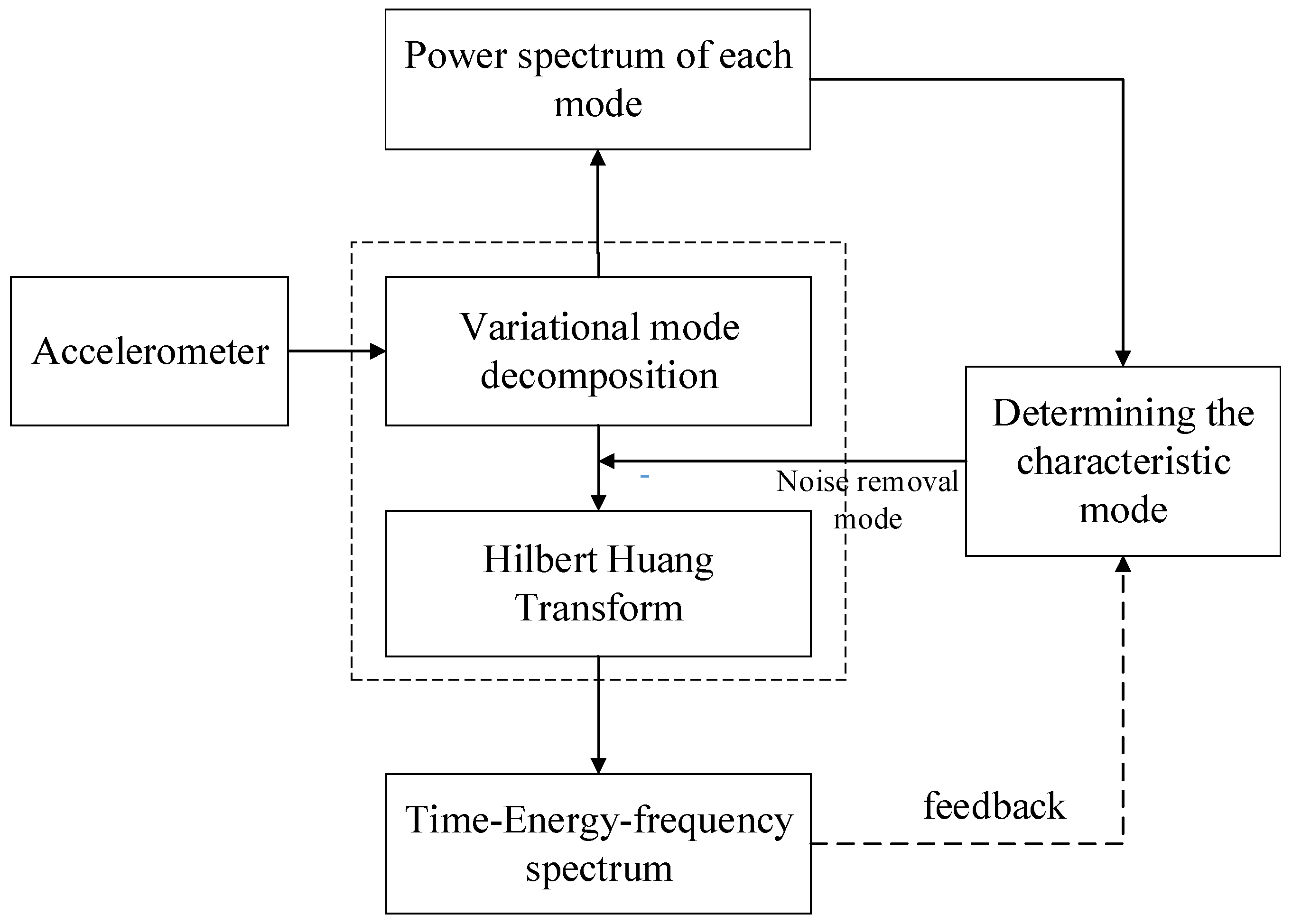
Variational mode decomposition (VMD) was put forward by Dragomiretskiy, K. and Zosso, D.in 2014 as a new method of time–frequency analysis based on traditional EMD [23]. The basic concept of VMD is to determine the center frequency and bandwidth of each IMF by searching for the optimal solution of the optimal function iteratively and decompose each IMF of frequency self-adaptively [24]. Research has shown that VMD could overcome the uncertainty of EMD in the center frequency and bandwidth and fundamentally reduce the endpoint effect and mode mixing. The basic steps of constructing the VMD objective function are as follows:

Analytic signals of each IMF are obtained by Hilbert transform to obtain a one-sided spectrum.

$$\left(\delta \left(t\right)+\frac{j}{\pi t}\right)·{\mu }_k\left(t\right)$$

(7)

where ${\mu }_k\left(t\right)$ is the kth IMF, and $\delta \left(t\right)$ stands for the pulse signal.

To modulate the spectrum of each mode to baseband, the exponential term $e^{-j{\omega }_{k}t}$ is added to the analytical signal of each IMF.

$$\left[(\delta \left(t\right)+\frac{j}{\pi t})·{\mu }_k\left(t\right)\right]e^{-j{\omega }_{k}t}$$

(8)

where ${\omega }_k$ denotes the estimated center frequency of the kth IMF.

Calculate the gradient of the 2-norm of the above functions and construct the following constraint model:

$$\{\begin{array}{c}\underset{\left\{u_k\right\},\left\{{\omega }_k\right\}}{\min }\left\{{\displaystyle {\displaystyle \sum }_k}\Vert {\partial }_t\left[\left(\delta \left(t\right)+\frac{j}{\pi t}\right)u_k\left(t\right)\right]e^{-j{\omega }_{k}t}{\Vert }_2^2\right\}\\ s.t. {\displaystyle {\displaystyle \sum }_k}{u}_k=f\end{array}$$

(9)

where $\left\{{\mu }_k\right\}$ is the set of each IMF, and $\left\{{\omega }_k\right\}$ indicates the center frequency of each IMF. Continuous iteration is carried out to optimize the above constraint model, and each center frequency and bandwidth are searched to self-adaptively decompose signal frequency.

To solve the optimal solution of the constraint model, the constrained variational problem can be transformed into an unconstrained variational problem by introducing quadratic penalty factor $\alpha$ and Lagrange multiplier $\lambda \left(t\right)$, the extended Lagrange expression is as follows:

$$\begin{gathered} L\left(\left\{u_k\right\},\left\{w_k\right\},\lambda \right)= \\ \alpha {\displaystyle \sum }_k\Vert {\partial }_t\left[(\delta \left(t\right)+\frac{j}{\pi t})·{\mu }_k\left(t\right)\right]e^{-j{\omega }_{k}t}{\Vert }_2^2+\Vert f\left(t\right)-{\displaystyle \sum }_k{u}_k\left(t\right){\Vert }_2^2+⟨\lambda \left(t\right), f\left(t\right)-{\displaystyle \sum }_k{u}_k\left(t\right)⟩ \end{gathered}$$

(10)

where $\alpha$ is the quadratic penalty factor, which can ensure signal accuracy in the presence of Gaussian noise. $\lambda \left(t\right)$ is the Lagrange multiplier, which can maintain strict constraint conditions. An alternate direction multiplier algorithm is used to solve the extended Lagrange function by alternating updates $u_k$,$w_k$,$\lambda$ to find “saddle point” of extended Lagrange expression [23].

2.3. VMD–HHT Model

Since VMD could weaken the inherent end effect and mode aliasing of EMD, a new approach of VMD–HHT time–frequency analysis is suggested in this paper by replacing EMD with VMD. First, the acceleration data were decomposed using VMD. Secondly, the power spectrum density (PSD) was used to extract each mode frequency. As a result, the frequency range of dynamic responses could be defined, and the noise modes were eliminated. Then, the time–frequency–energy spectrum could be gained by employing HHT to extracted modes. Lastly, assisted by the spectrum to adjust and determine feature modes, characteristic information of dynamic responses with high accuracy could be obtained in all directions. Figure 1 shows the process of the VMD–HHT-based characteristic extraction model.

To verify the VMD–HHT-based characteristic extraction model for dynamic responses, a set of data was simulated to compare the performance between traditional HHT and VMD–HHT in extraction. The analog data consisted of five sinusoidal signals with different amplitudes and frequencies (the frequencies were 1 Hz, 5 Hz, 10 Hz, 15 Hz, and 35 Hz, respectively) at a sampling frequency of 100 Hz, and the effect of random noise was also added, as shown in Figure 2.

As shown in Figure 3, HHT cannot extract characteristic information of accelerometer signals. In contrast, the VMD–HHT model can accurately separate frequencies of analog signals into each band (separation frequency is consistent with setting frequency) and qualitatively analyze frequency distribution of energy based on color. Moreover, the analog data were made up of time-invariant stationary signals with constant statistics along the time axis. According to previous analyses and research, even for accessible composite signals, HHT cannot separate characteristic information effectively. Its algorithm EMD would cause mode aliasing, while the VMD–HHT would not. Therefore, this paper proposes an HHT method using VMD instead of EMD, from now on referred to as VMD–HHT time–frequency analysis model.

3. Dynamic Responses Monitored by MIMU

It is appropriate to monitor dynamic response using MIMU due to the high sampling rate, which can reach up to 100 Hz–200 Hz. The displacement, velocity, and torsion angle responses can be calculated by mechanical arrangement using MIMU. However, low-cost MIMU has a relatively low measurement accuracy with a large gyroscope drift. By processing and analyzing the observed time-series data of accelerometer and gyroscope, real-time dynamic responses of offshore oil platforms can be provided. The monitoring accuracy can also be improved.

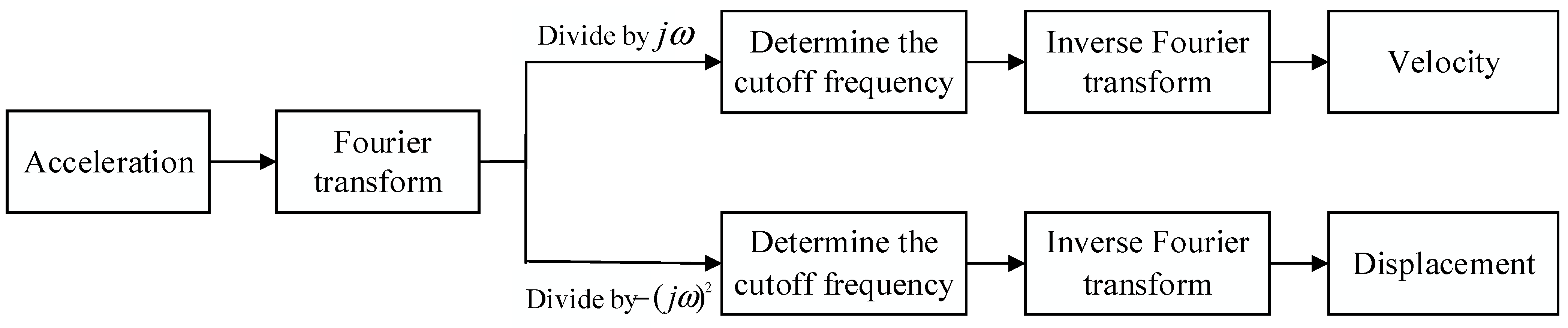
3.1. Accelerometer-Derived Displacement Reconstruction

The frequency-domain integration approach (FDIA) is based on Fourier transform, which derives from its integral property as follows:

$$ℱ\left[{{\displaystyle \int }}_{-\infty }^{t}a\left(t\right)dt\right]=\frac{1}{j\omega }·ℱ\left[a\left(t\right)\right]$$

(11)

where $ℱ$ represents the Fourier transform symbol, $a\left(t\right)$ denotes the acceleration signal, $j$ is the imaginary number, and $\omega$ means the frequency. The above formula illustrates that the Fourier transform of acceleration signal integration is equivalent to the Fourier transform of the signal divided by the factor $i\omega$, simplifying the complex integration into division.

In FDIA, the signal is transformed into a frequency-domain signal by Fourier transform, and the operation is completed in the frequency domain. The velocity and displacement information in the time domain is obtained by inverse Fourier transform. The calculation procedure is represented in Figure 4.

The frequency spectrum of the acceleration signal after Fourier transform can be expressed by

$$A\left(k\right)={\displaystyle \sum }_{n=0}^{N-1}a\left(n\right)e^{-j\left(2\pi nk/N\right)}$$

(12)

where $N$ is the number of acquisition points, $a\left(n\right)$ means the discrete expression of $a\left(t\right)$, and $n$ and $k$ stand for positive integers.

According to the formula, the single integration is obtained as follows:

$$V\left(n\right)=\frac{A\left(k\right)}{j\omega }={\displaystyle \sum }_{k=0}^{N-1}\frac{1}{j2\pi k\mathsf{\Delta }f}H\left(k\right)a\left(n\right)e^{-j2\pi nk/N}$$

(13)

The results of double integration are given by

$$X\left(n\right)=-\frac{A\left(k\right)}{{\omega }^2}={\displaystyle \sum }_{k=0}^{N-1}\frac{1}{-{\left(j2\pi k\Delta f\right)}^2}H\left(k\right)a\left(n\right)e^{-j2\pi nk/N}$$

(14)

As for $H\left(k\right)=\{\begin{array}{c}1 \left(f_d\le k\Delta f\le f_u\right)\\ 0 \left(other\right)\end{array}$, $\Delta f$ is the frequency resolution while $f_d$ and $f_u$ are the upper and lower cutoff frequencies, respectively. After all Fourier components of different frequencies are calculated according to the frequency-domain relationship, time-domain signals can be obtained by inverse Fourier transform.

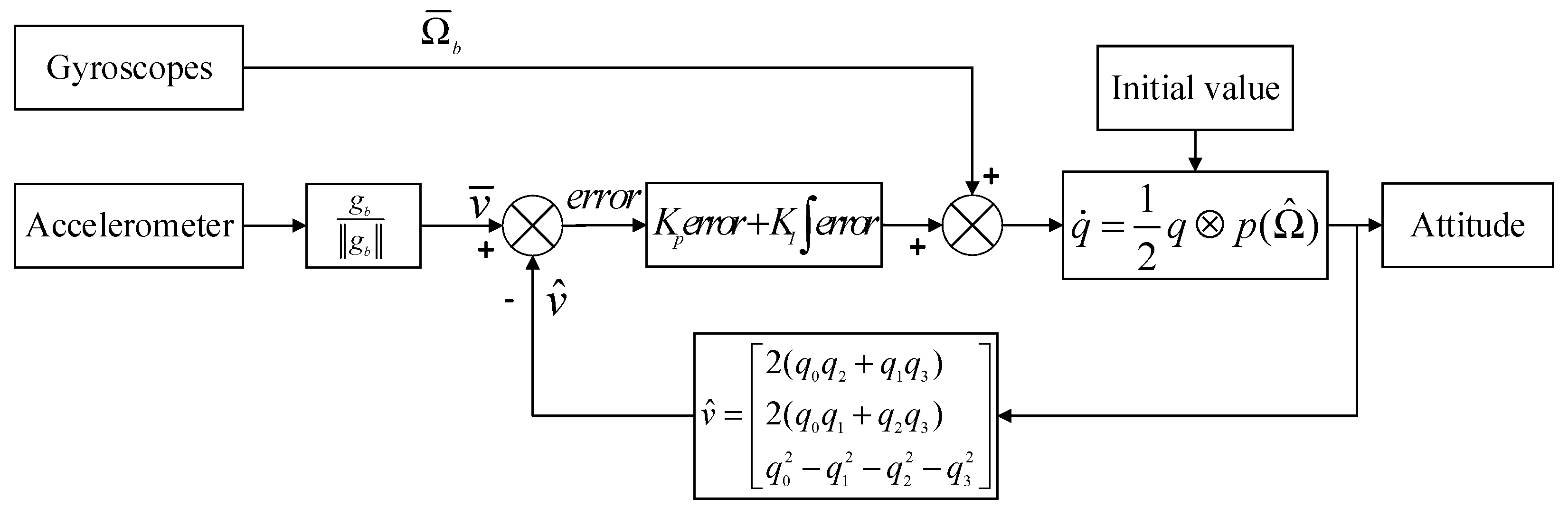
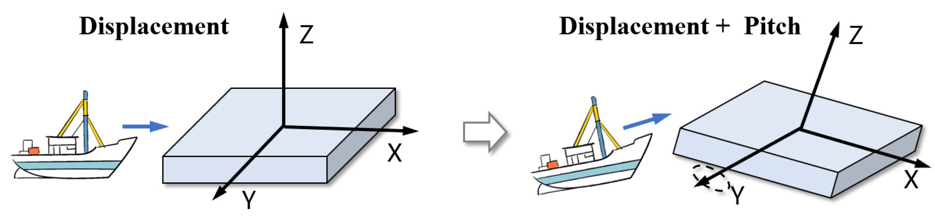
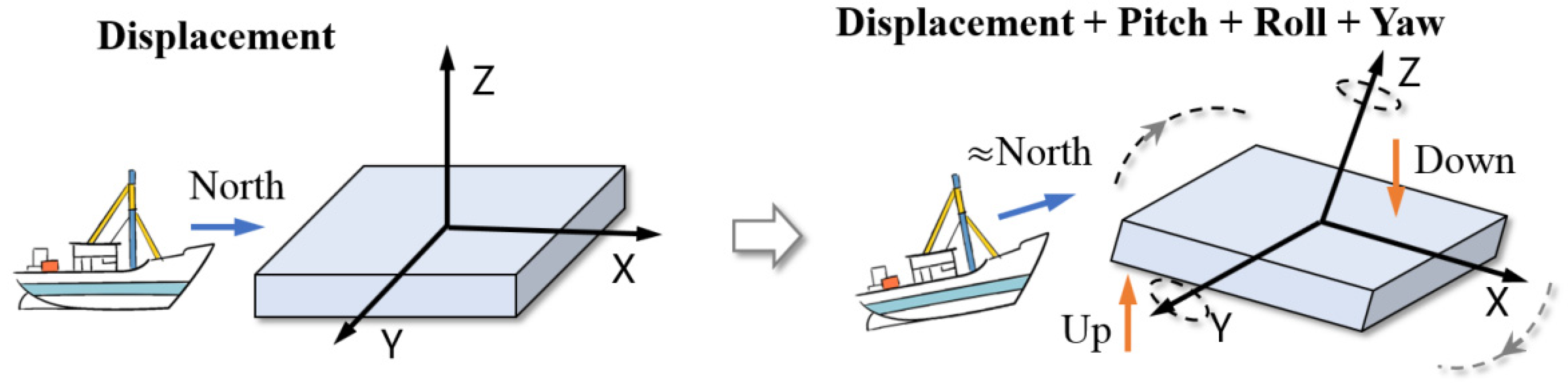
3.2. Gyro-Derived Torsion Reconstruction

The Mahony complementary filter has been routinely used to calculate torsion angle after its first successful trial in estimating the torsion angle of UAV accurately [25]. Since it is easy to understand and less time consuming, this algorithm is widely used in engineering applications. The basic idea behind the Mahony complementary filter is that when the carrier is at a static state, the theoretical value of the gravity acceleration component is ${\left[00g\right]}^T$ in a geographical coordinate system. Then, the matrix of ${\left[00g\right]}^T$ is transformed under the carrier coordinate system to compare with the measurements of the accelerometer. Thus, this deviation is the error between the torsion angle integrated by gyroscope and measured accelerometer, respectively. The steps of the algorithm are as follows:

(1)

The accelerometer is normalized to a single vector $\frac{g_b}{\Vert g_b\Vert }$.

(2)

The acceleration data in the geographical coordinate system are converted to the carrier coordinate system, and the estimation in the carrier coordinate system is given by

$$\widehat{v}=\left[\begin{array}{c}2\left({\widehat{q}}_1{\widehat{q}}_3+{\widehat{q}}_0{\widehat{q}}_2\right)\\ 2\left({\widehat{q}}_2{\widehat{q}}_3+{\widehat{q}}_0{\widehat{q}}_1\right)\\ {\widehat{q}}_0^2-{\widehat{q}}_1^2-{\widehat{q}}_2^2+{\widehat{q}}_3^2\end{array}\right]$$

(15)

where $q$ is quaternions.

(3)

The deviation between the acceleration estimation $\widehat{v}$ and the measurements by accelerometer $\overline{v}$ is the error item between the integrated torsion angle of the gyroscope and the torsion angle measured by the accelerometer. The value $errror$ can be expressed by the cross product.

$$errror=\widehat{v}\times \overline{v}$$

(16)

(4)

The corrected torsion angle can be obtained based on a PI controller using the results from the previous step,

$$\hat{\mathsf{\Omega }}={\overline{\Omega }}_b+K_{p}error+K_I{{\displaystyle \int }}^{\text{}}error$$

(17)

where ${\overline{\Omega }}_b$ is the torsion angle obtained by gyro integration, while $K_p$ and $K_I$ are the PI control param.

(5)

The quaternion differential equation can be solved by using the corrected torsion angle $\hat{\mathsf{\Omega }}$ (See Formula (8)), and the quaternion can be updated to calculate the theoretical estimation of the accelerometer (transfer to Equation (2)).

$$\dot{q}=\frac{1}{2}q\otimes p\left(\hat{\mathsf{\Omega }}\right)$$

(18)

The algorithm flowchart of Mahony complementary filtering is presented in Figure 5.

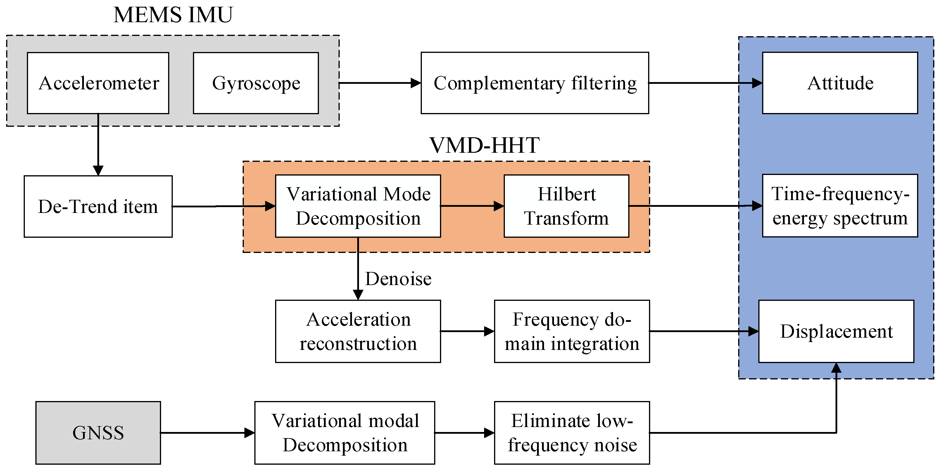
3.3. The Schematic to Monitor Dynamic Responses Based on VMD–HHT Characteristic Extraction Model

A multidimensional characteristic extraction method based on VMD–HHT is introduced to monitor dynamic responses of offshore oil platforms. First, VMD was applied to extract the frequency component of the dynamic response, and the noise component could thus be eliminated. Then, HHT was used to extract multidimensional dynamic response characteristics of time, frequency, and energy using the cleaned accelerometer data. Finally, dynamic displacement responses were calculated by the FDIA based on the cleaned data. To assess the reliability of dynamic displacement responses obtained by accelerom, GNSS data are given for comparison. In addition, to obtain torsion angle changes of offshore oil platforms, the complementary filtering algorithm was applied using six-degree of freedom of MIMU. The flowchart for dynamic responses based on VMD–HHT using MIMU is summarized in Figure 6.

4. Simulation Shaking-Table Tests

4.1. Simulation Shaking Table

To verify the reliability of the VMD–HHT model and displacement reconstruction method, a series of simulation shaking-table tests were performed using accelerometer in the MIMU. The simulation shaking table (see in Figure 7) comprised a platform framework, steel plates for equipment, two mutually perpendicular screw rods, a servo motor, a control panel, and a power box. The platform frame is 1.2 m long, 1.2 m wide, and 0.5 m high, and the steel plates for equipment are 0.3 m long, 0.1 m wide, and 0.02 m thick. To install the GNSS antenna, a screw hole was drilled through the steel plates; moreover, the screw rods were driven by the servo motor when the steel plates move horizontally with screw rods. In addition, the control system of the shaking table adjusted the vibration amplitude and frequency through the control panel.

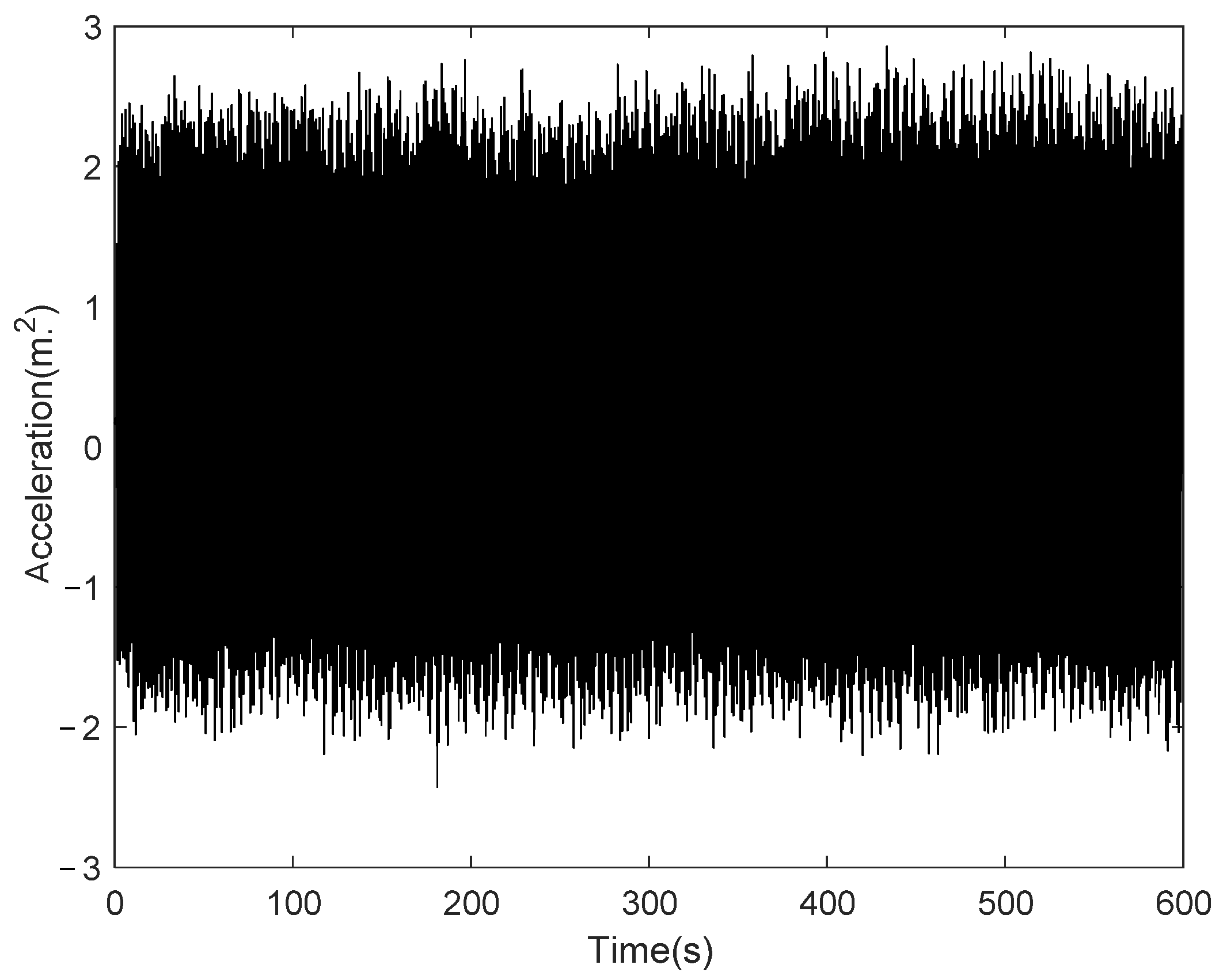
4.2. Data Collection

On 31 December 2020, the experimental measurements of dynamic displacement monitoring were carried out on the platform located in the south square of Beijing University of Civil Engineering and Architecture (BUCEA). The equipment used in the tests includes the shaking table, a GNSS deformation monitoring system independently developed by BUCEA, the ADIS16505 IMU (inertial measurement unit) produced by Analog Devices, Inc. (containing an accelerometer and gyroscope, but only the accelerometer data were used in this test) and laptops. The param of GNSS and accelerometer are shown in the following

Table 1. Principal specifications of GNSS and accelerometer.

Equipment	Performance
GNSS	Signal Tracking	BDS: B1/B2; GPS:L1/L2 GLONASS: L1/L2; GALILEO:E1/E5b
	RTK (RMS)	Horizontal: $\pm$8 mm + 1 ppm Vertical: $\pm$15 mm + 1 ppm
	Updating Frequency	5 Hz
Accelerometer	Dynamic Range	$\pm 78.4 \mathrm{m}/{\mathrm{s}}^2$
	Bias Stability	$26.5\times {10}^{-6}\mathrm{m}/{\mathrm{s}}^2$
	Noise Density	$167\times {10}^{-6}\mathrm{m}/{\mathrm{s}}^2/\surd \mathrm{Hzrms}$
	Updating Frequency	100 Hz

.

Two sets of equipment, the GNSS and accelerometer, were attached to the shaking table using a metal plate. The connecting line between the centers of MIMU and GNSS antenna was directed toward north–south. Since the accelerometer was located toward the northern GNSS antennas at the distance of 10 cm using a northeast down system, the installation direction of the X-axis would point to the north. The layout of monitoring systems and monitoring points are shown in Figure 8.

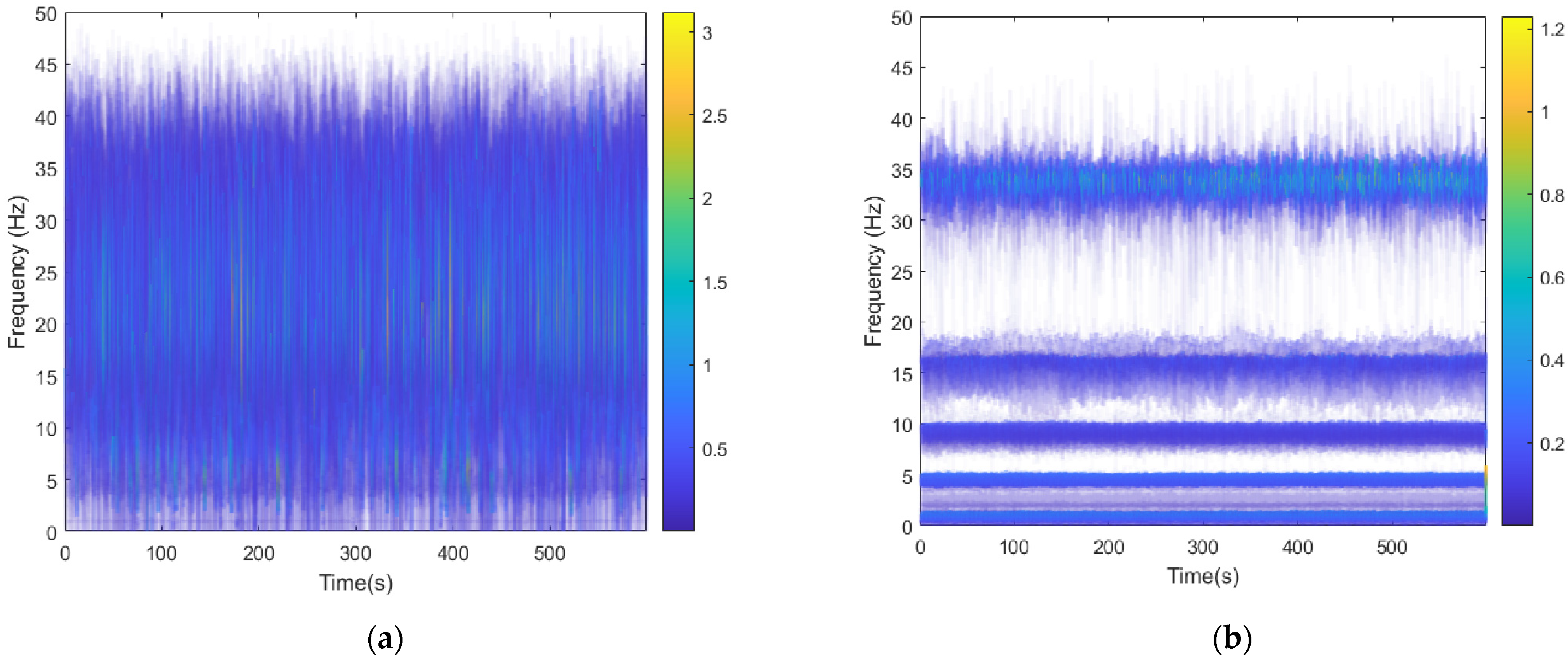
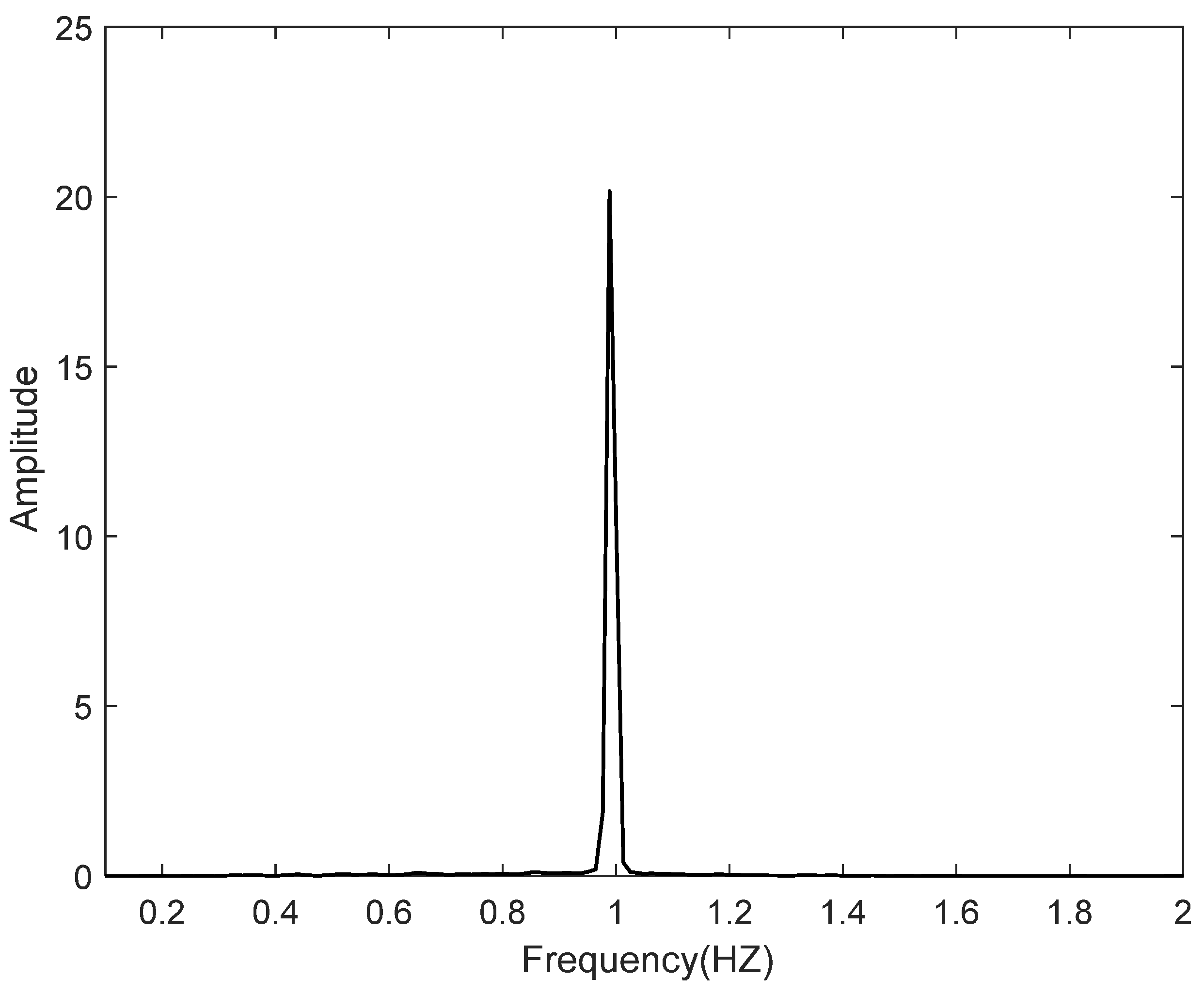
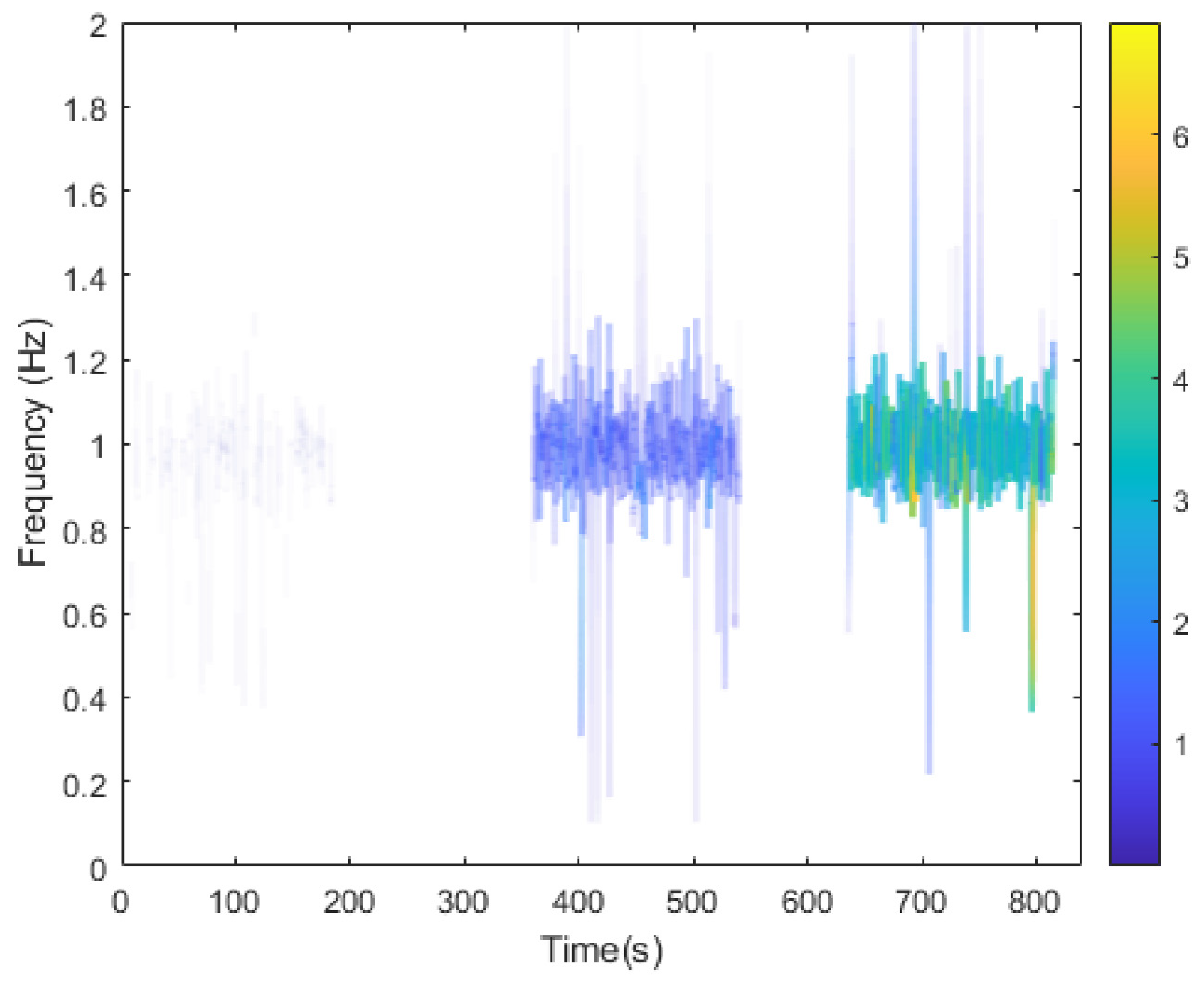
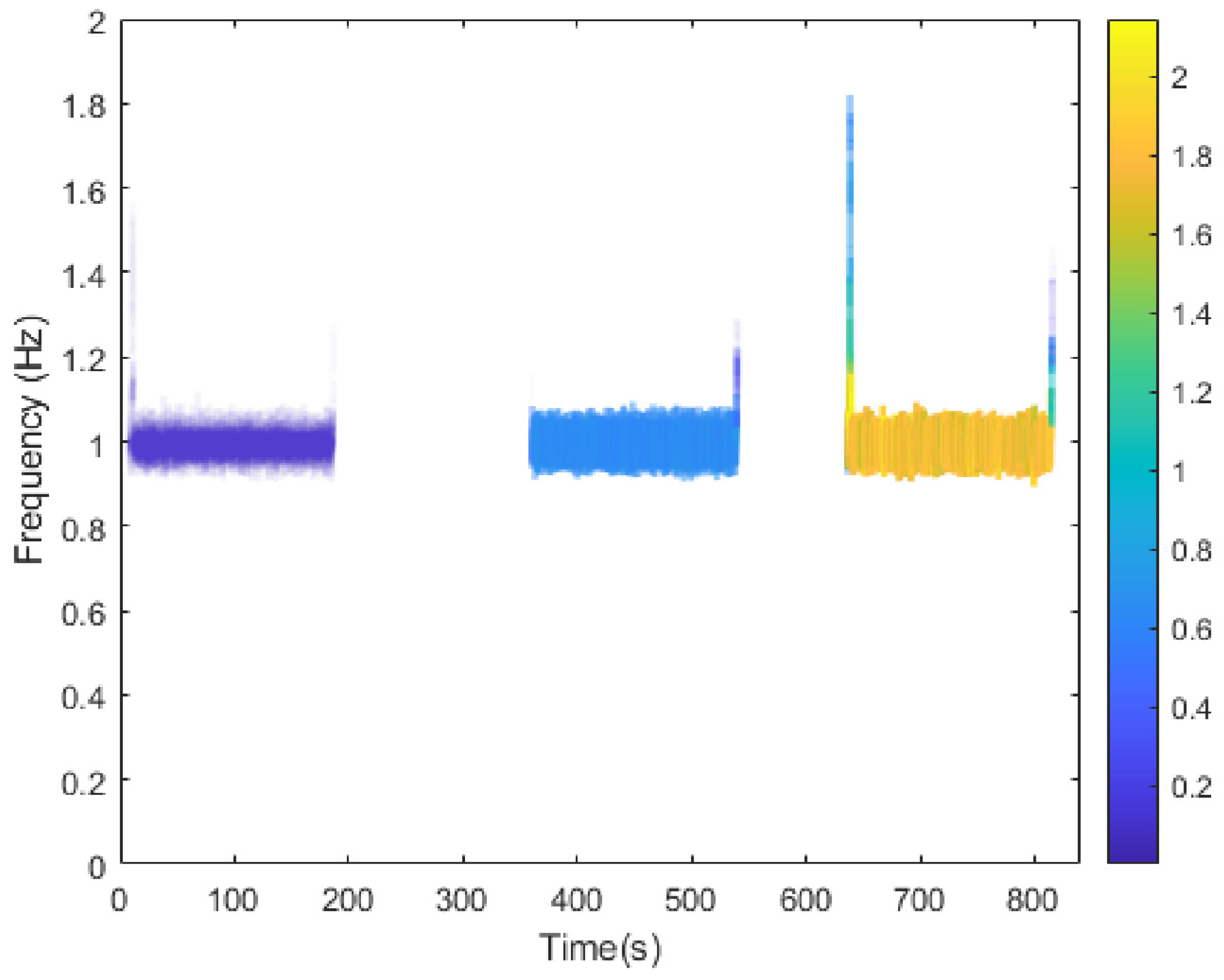
4.3. Comparison of PSD, HHT, and VMD–HHT

To illustrate the advantages of the VMD–HHT model in the time domain and energy domain compared with PSD and HHT, three groups of tests were designed with time sequence amplitudes of 10 mm, 30 mm, and 50 mm. A GNSS receiver using a 5 Hz sampling rate and an accelerometer using a 100 Hz sampling rate were used to obtain the three original data sets for comparison.

The shaking table tests were conducted for 10 min (each test lasted approximately 3 min). The test site had an open view of the sky, thus avoiding multipath effects. Additionally, during the experiments, there was no wind to prevent wind-induced frequency noise. Figure 9 gives the frequency extract from three vibration events using the method of PSD; as seen from Figure 9, the frequency response peaked at 1 Hz is consistent with the vibration frequency of the shaking table. However, the time of the three groups of tests with amplitudes of 10 mm, 30 mm, and 50 mm is unknown from Figure 9 due to the frequency of all tests are 1 Hz.

HHT and VMD–HHT methods can separate each event in the time dimension and reflect the intensity of each event (Figure 10). It can be seen that the frequency range is about 1 Hz, and the intensity of three events is gradually strengthening, corresponding to amplitudes at 10 mm, 30 mm, and 50 mm. Comparing Figure 10 and Figure 11 show that the HHT spectrum is noisier than the VMD–HHT spectrum. We can also observe that the intensity displayed in the HHT spectrum is smaller than the VMD–HHT spectrum, and the latter is more clearly detected. However, the frequency values at the beginning and end of each signal also reach higher values, especially the signal with amplitude at 50 mm. It is probably caused by endpoint effect. Overall, VMD–HHT can extract the characteristics of time, frequency, and energy more reliably than HHT.

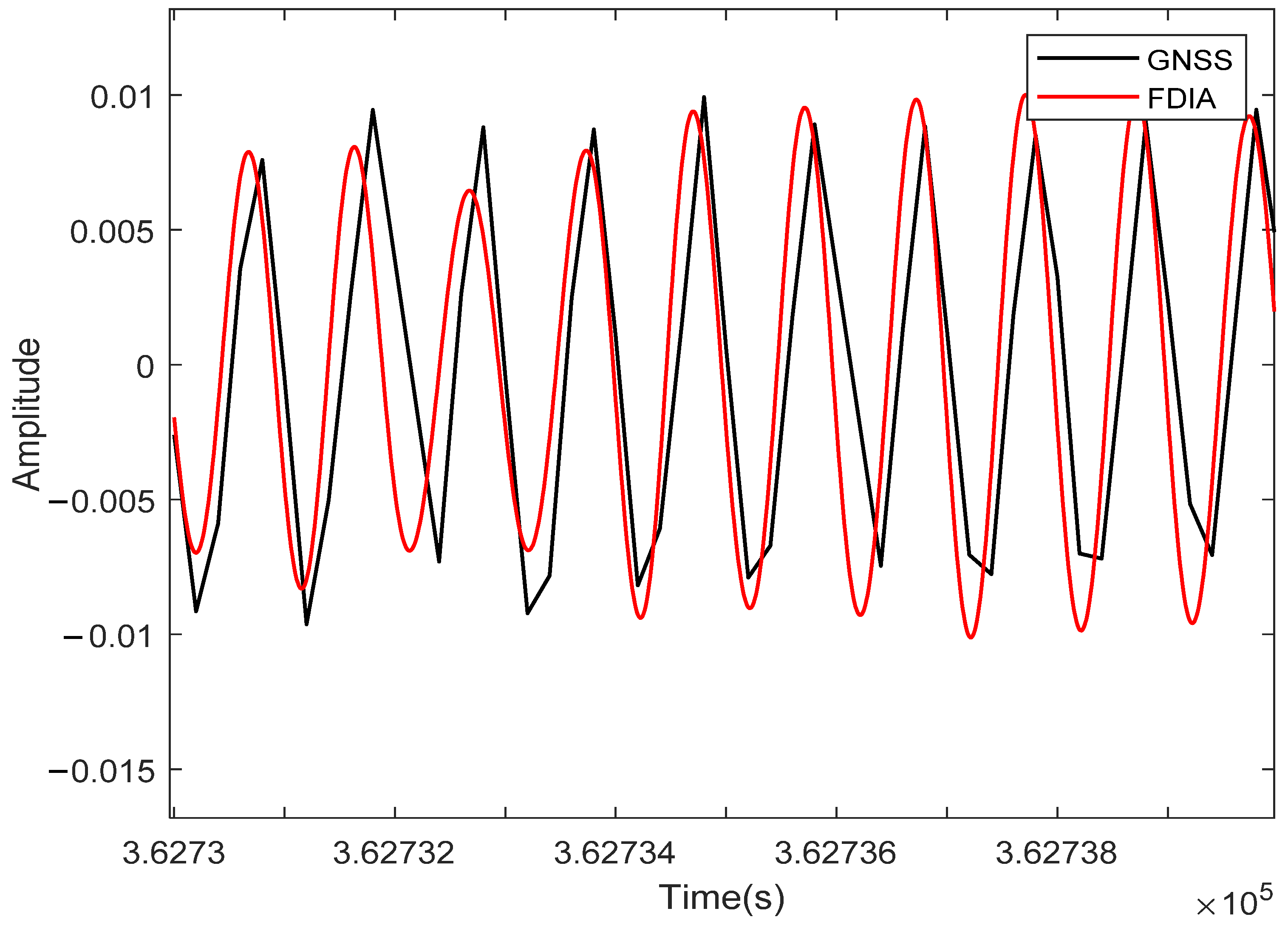
4.4. Reconstruction of Dynamic Displacement Using FDIA Based on the VMD–HHT Model and GPS

To assess the effectiveness and accuracy of FDIA based on the VMD–HHT model, displacements measured by GNSS are given for comparison. Firstly, the VMD approach was applied to remove residual and high-frequency noise from accelerometer data. Then, FDIA was used to obtain vibration displacements based on the cleaned data proposed by VMD. Figure 12 shows the displacement comparison of GNSS and FDIA; as seen from Figure 12, there is a high correlation between GNSS and FDIA. It is evident that the vibration amplitude is about 10 mm, and frequency is about 1 Hz, which is consistent with the set param. It can be concluded that VMD–HHT-based FDIA has successfully calculated the vibration displacements.

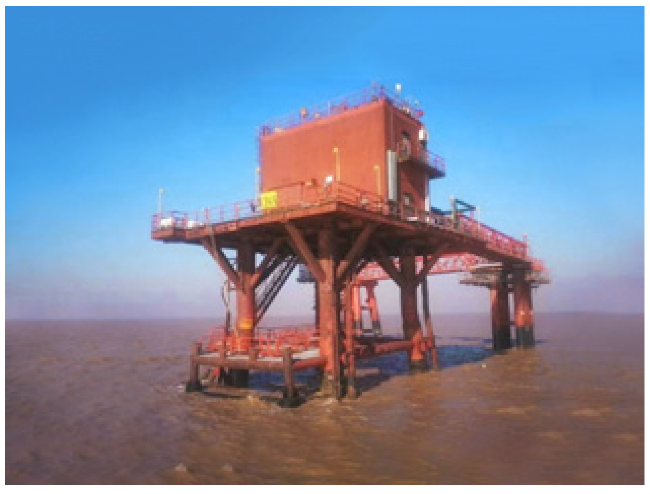
5. Trial Analysis of CB4A Offshore Oil Platform

Located at 38°8′39″ north latitude and 118°50′38″ east longitude, the CB4A offshore oil platform lies in the Yellow River Delta along the coast of the Bohai Sea. It is a fixed offshore oil platform in Shengli Oilfield at Dongying City with a total area of 700 ${\mathrm{m}}^2$(see in Figure 13). The sea area near the platform is windy all year round, affected by the southeast Pacific monsoon and the northwest monsoon of the Asian continent. More specifically, as frequently affected by the monsoon of the Asian continent, the offshore oil platform also suffers from heavy wind all year round. In addition, being close to the maritime transportation hub, the platform is under heavy traffic. As a result, ship collisions occur from time to time, and thus, the monitoring of offshore oil platforms becomes exceptionally urgent.

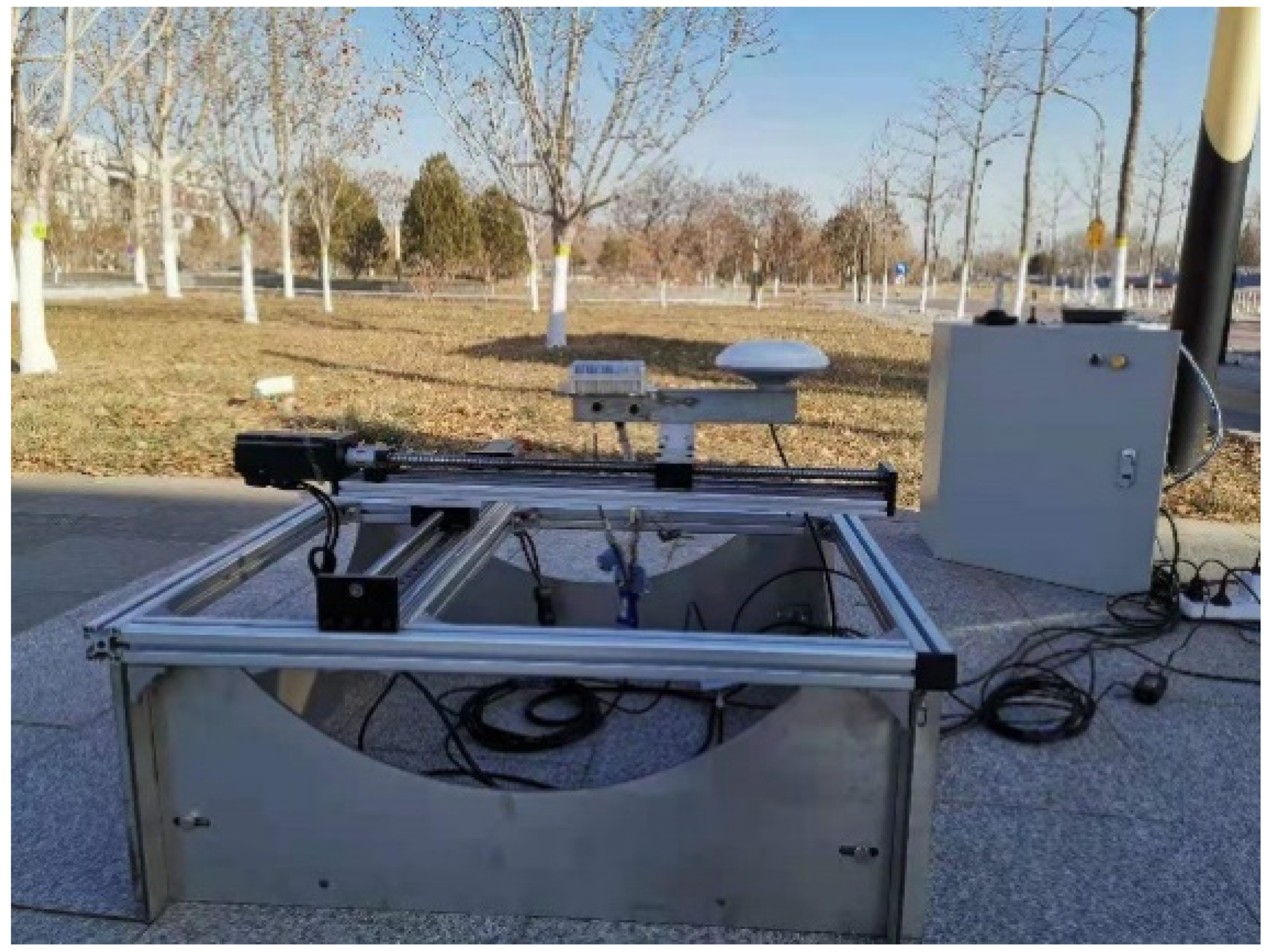
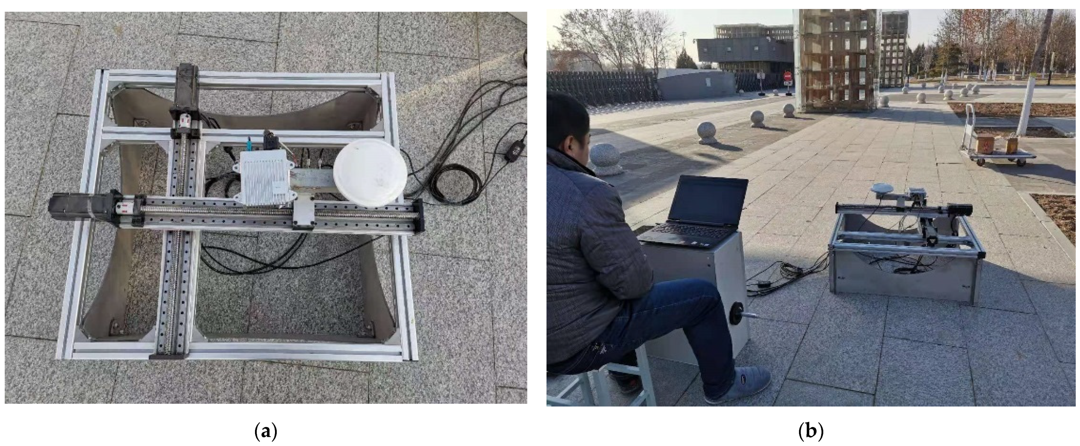
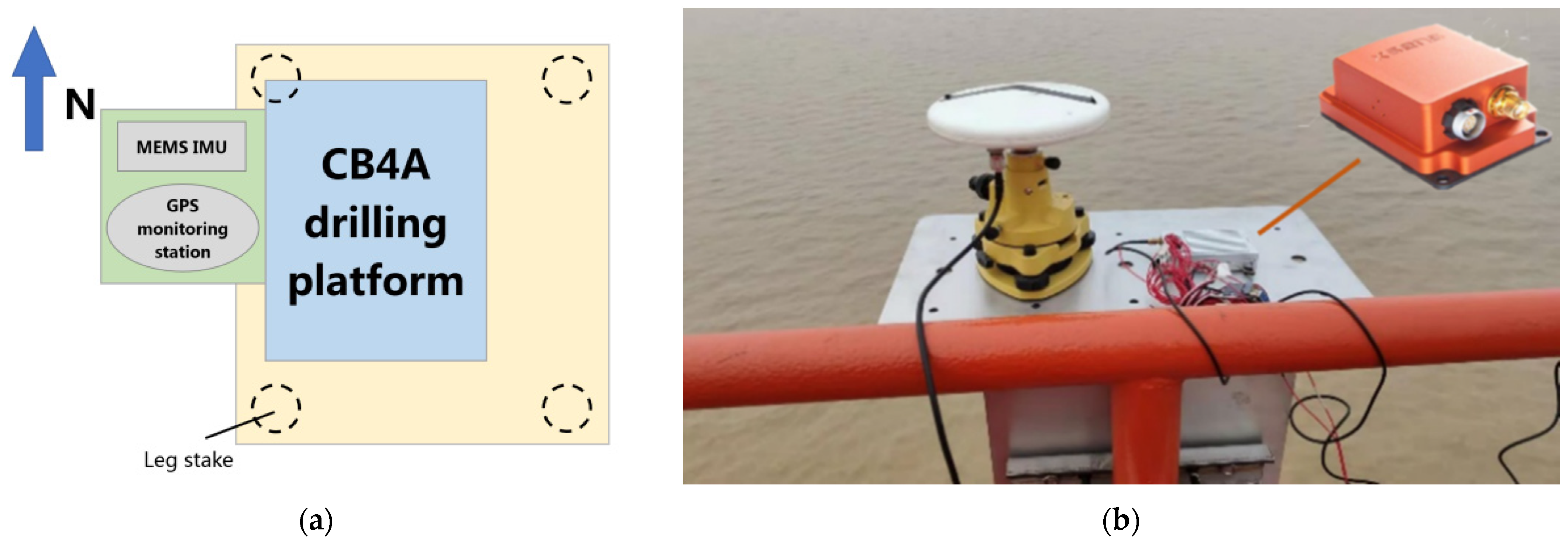
5.1. Equipment for Monitoring Dynamic Responses

MIMU used in the dynamic responses monitoring trial were from Mti300 inertial sensors by Xsens Technologies B.V. of the Netherlands (as shown in the upper right corner of Figure 14b). The specifications of Mti300 are given in

Table 2. Performance index for Mti300.

Index Item	Gyroscope	Accelerom
Standard full range	±450 °/s	±20 g
Initial bias error (one year)	0.2 °/s	5 mg
In-run bias stability	10 °/h	15 µg
Bandwidth (−3 dB)	415 Hz	375 Hz
Noise density	0.01 °/s/√Hz	60 µg/√Hz
g-sensitivity (calibrated)	0.003 °/s/g	N/A
Nonorthogonality	0.05 deg	0.05 deg
Nonlinearity	0.01%	0.1%

. Furthermore, to demonstrate the accuracy and reliability of dynamic displacement responses by MIMU, a GPS monitoring system independently developed by BUCEA was installed on CB4A offshore oil platform. GPS RTK technology was used in this trial. The specifications of GPS are given in

Table 3. Performance index for GPS.

Tracking Signal	BDS B1/B2/B3
	GPS L1/L2/L5
	GLONASS /L1/L2
	GALILEO E1/E5a/E5b
	QZSS L1/L5
	SBAS L1
Single(RMS)	Plane: $\pm$1.5 m; Altitude: $\pm$3 m
DGPS(RMS)	Plane: $\pm$0.4 m; Altitude: $\pm$0.8 m
RTK(RMS)	Plane: $\pm$8 mm + 1 ppm Altitude: $\pm$15 mm + 1 ppm
Sampling rate	5 Hz

. The layout of the monitoring systems and the monitoring point for dynamic responses are indicated in Figure 14. Two sets of equipment were positioned at the northwest corner of the platform roof and attached to the roof railing by a sheet iron. The connecting line between the centers of MIMU and GPS antenna was directed toward the north–south. The MIMU was placed 20 cm to the north of the GPS antenna navigated by the NED coordinate system, and its X-axis was installed to the north.

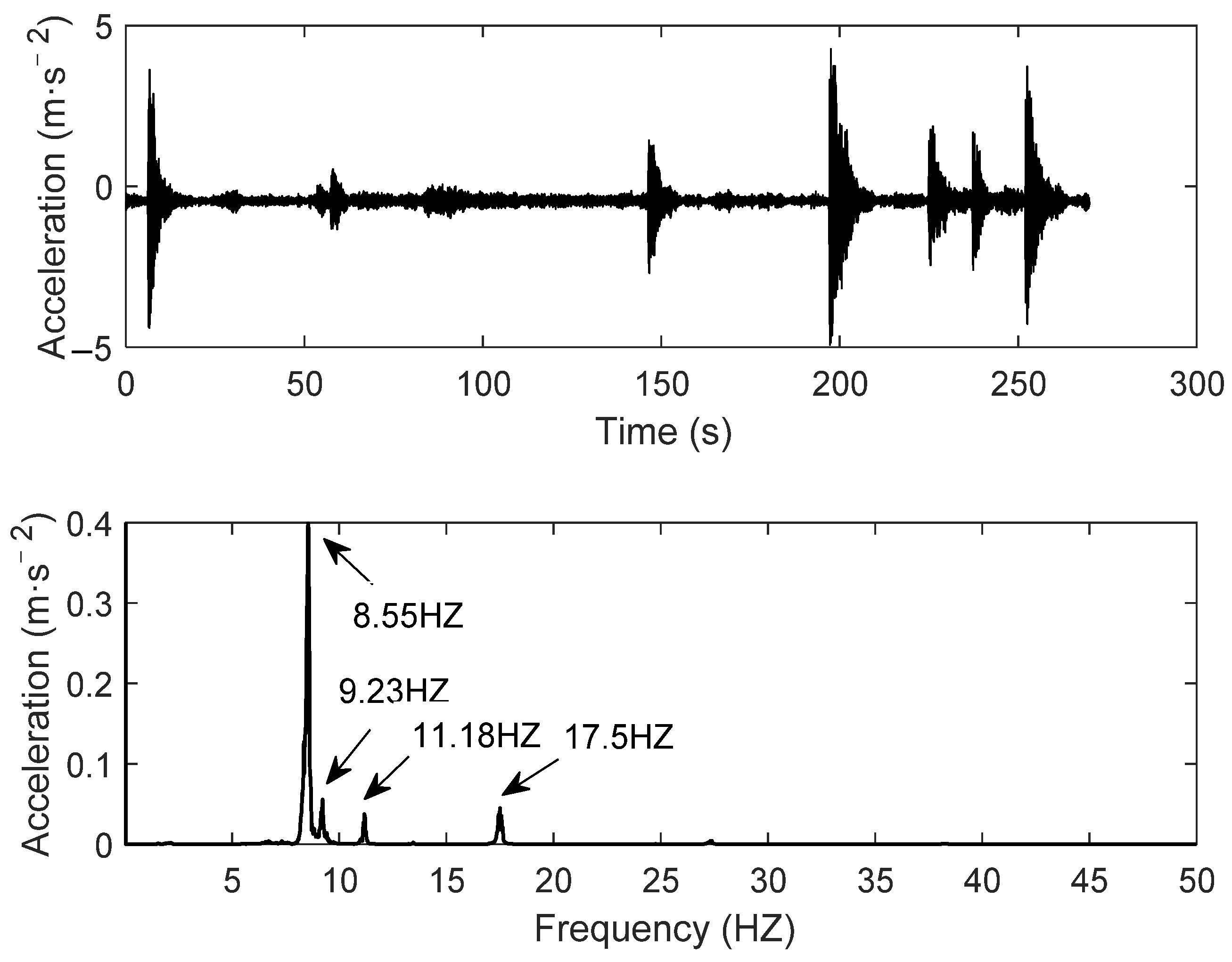
5.2. Data Acquisition

The monitoring trial of the CB4A offshore oil platform was carried out in Dongying city, Shandong Province, on 3 December 2019. The MIMU and GPS data sampling frequencies were set at 100 Hz and 5 Hz, respectively, with a 4.5 min sampling time (GPS time: 200088.0–200358.0). We planned to design an experiment for researching the dynamic response of offshore oil platforms induced by wind and waves from the beginning. However, as CB4A offshore oil platform was a stable rigid body at the height of only 7 m, it would be difficult to produce dynamic responses caused by slight winds or waves. Unfortunately, the weather was suitable, with no strong winds and/or waves during the tests. Thus, wind and waves were replaced with ship collision events. The ship collision experiment was conducted on a calm afternoon, which would avoid the influence of wind and waves. A small ship, about 5 m long, successive hit the leg of the platform traveling from south to north at a speed of 20 km per hour. When the small ship started to hit the leg of the platform, the experimenter recorded the current Beijing standard time. The continuous collision lasted for about 4 min. Eight collisions were made, and the time interval of each impact was less than 1 min. The time of each impact was recorded manually and is shown in

Table 4. Record schedule of ship collision.

Collision	First	Second	Third	Fourth	Fifth	Sixth	Seventh	Eighth
Time	15:34:37	15:35:28	15:36:00	15:36:58	15:37:30	15:37:51	15:38:17	15:38:46
GPS Period	200094.6	200145.6	200177.6	200235.6	200267.6	200290.8	200314.6	200343.8

.

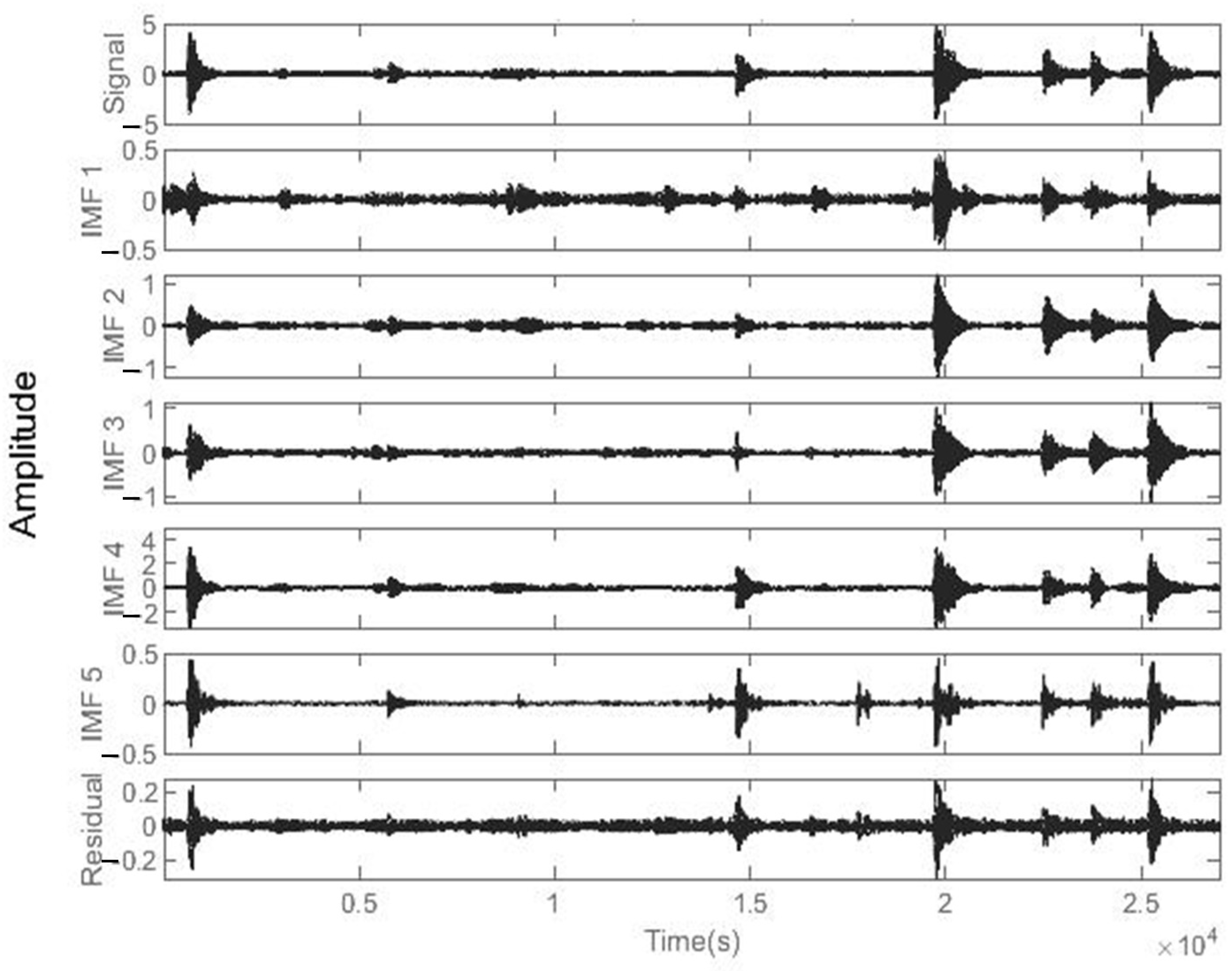
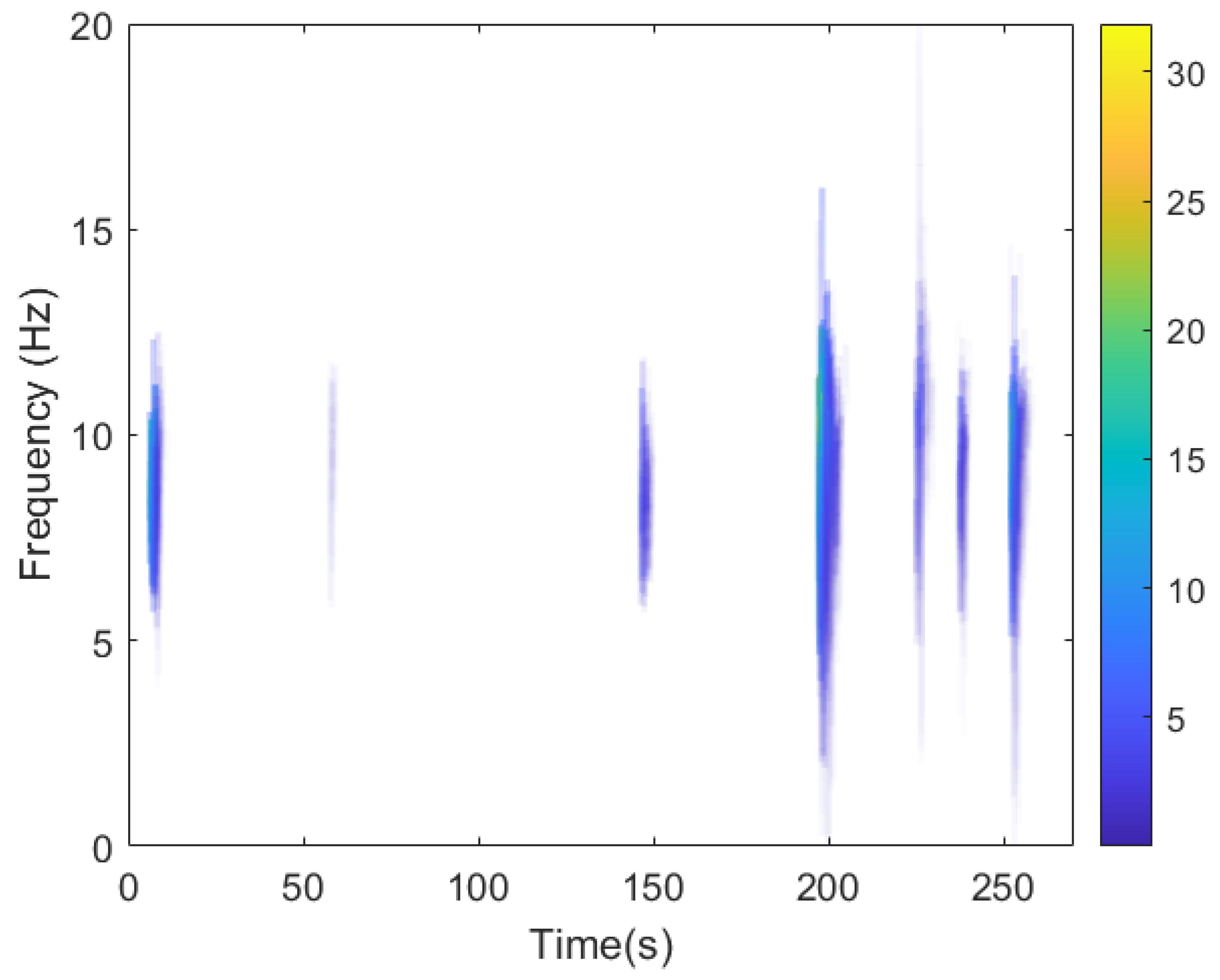
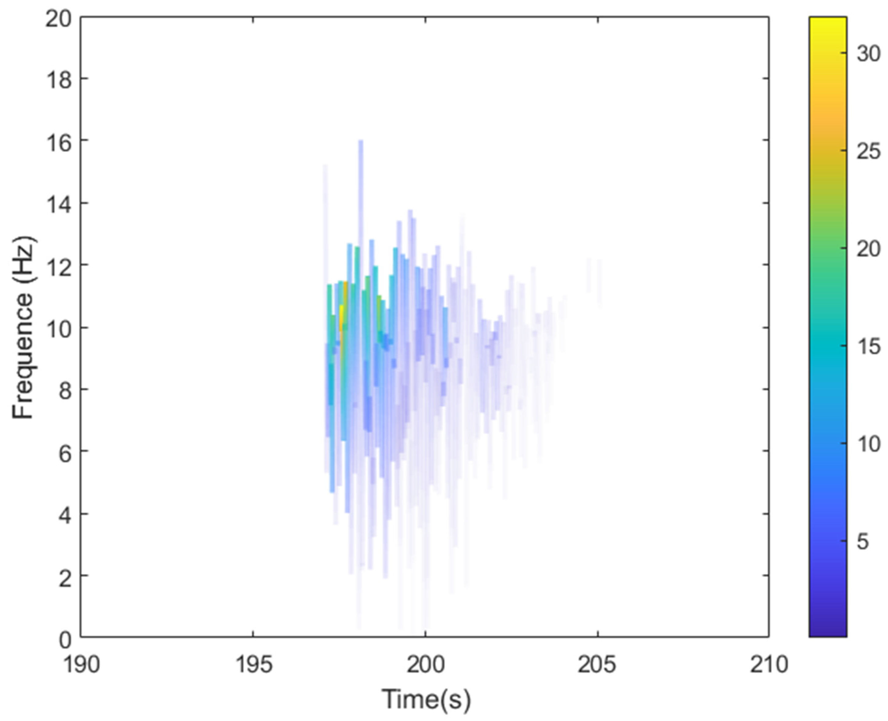
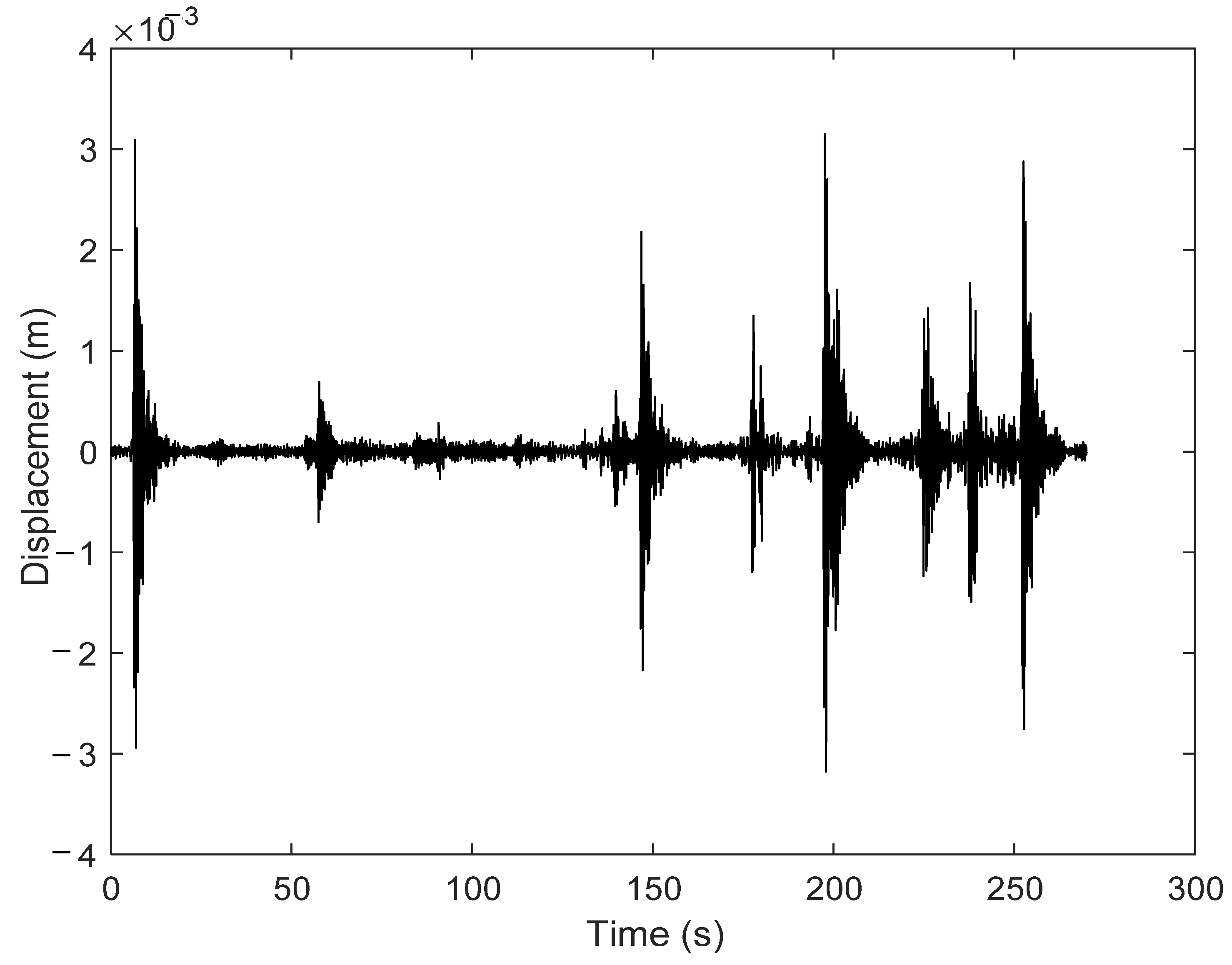
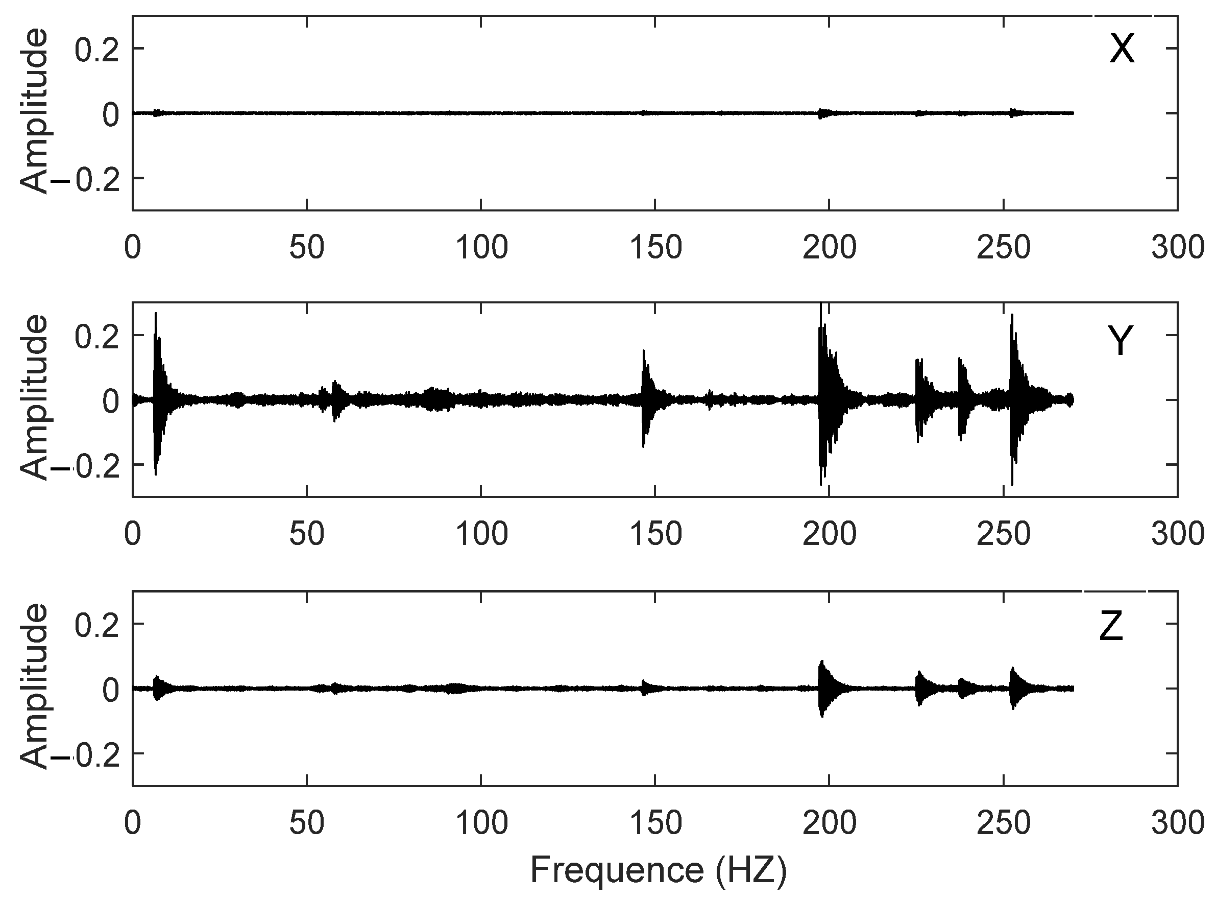
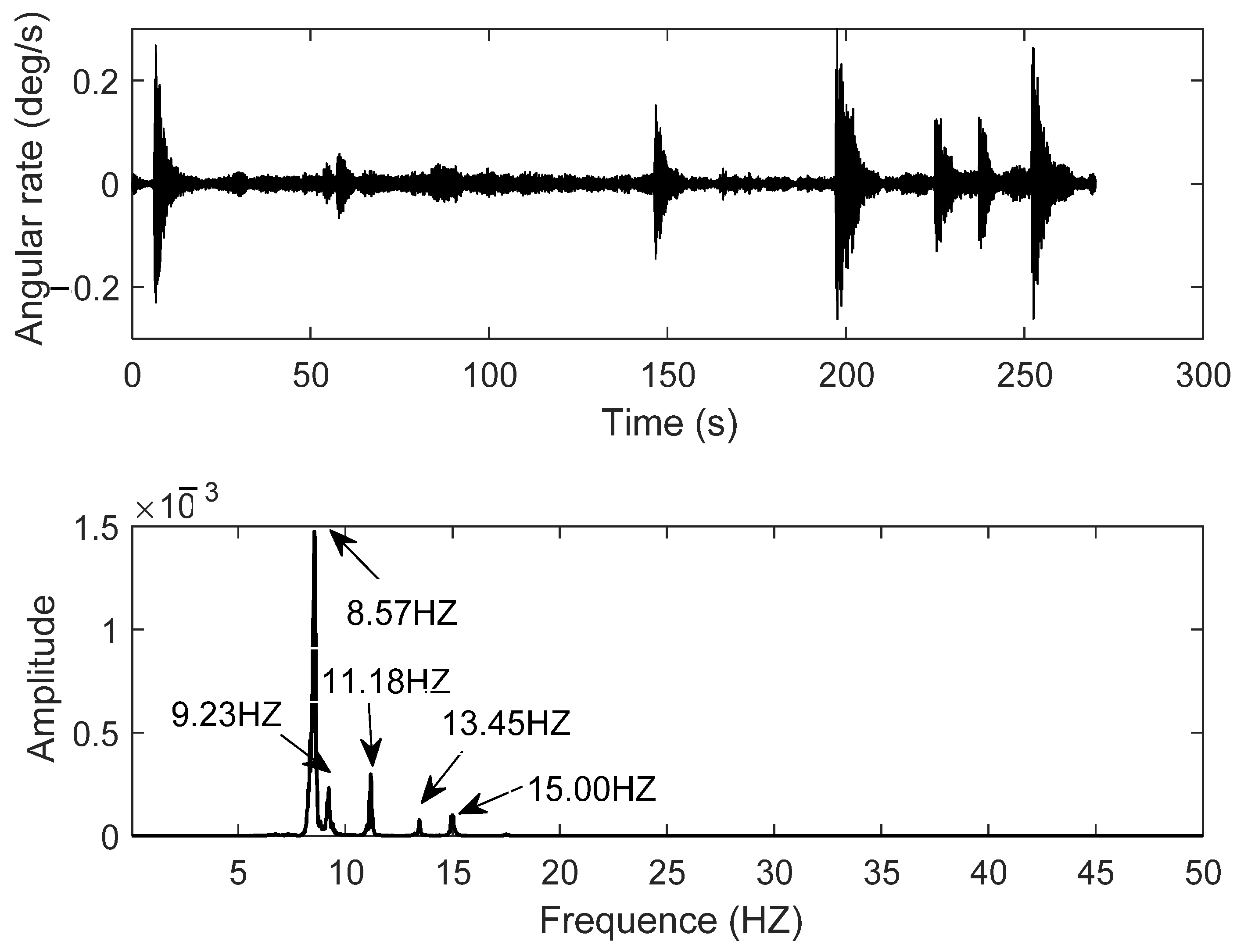
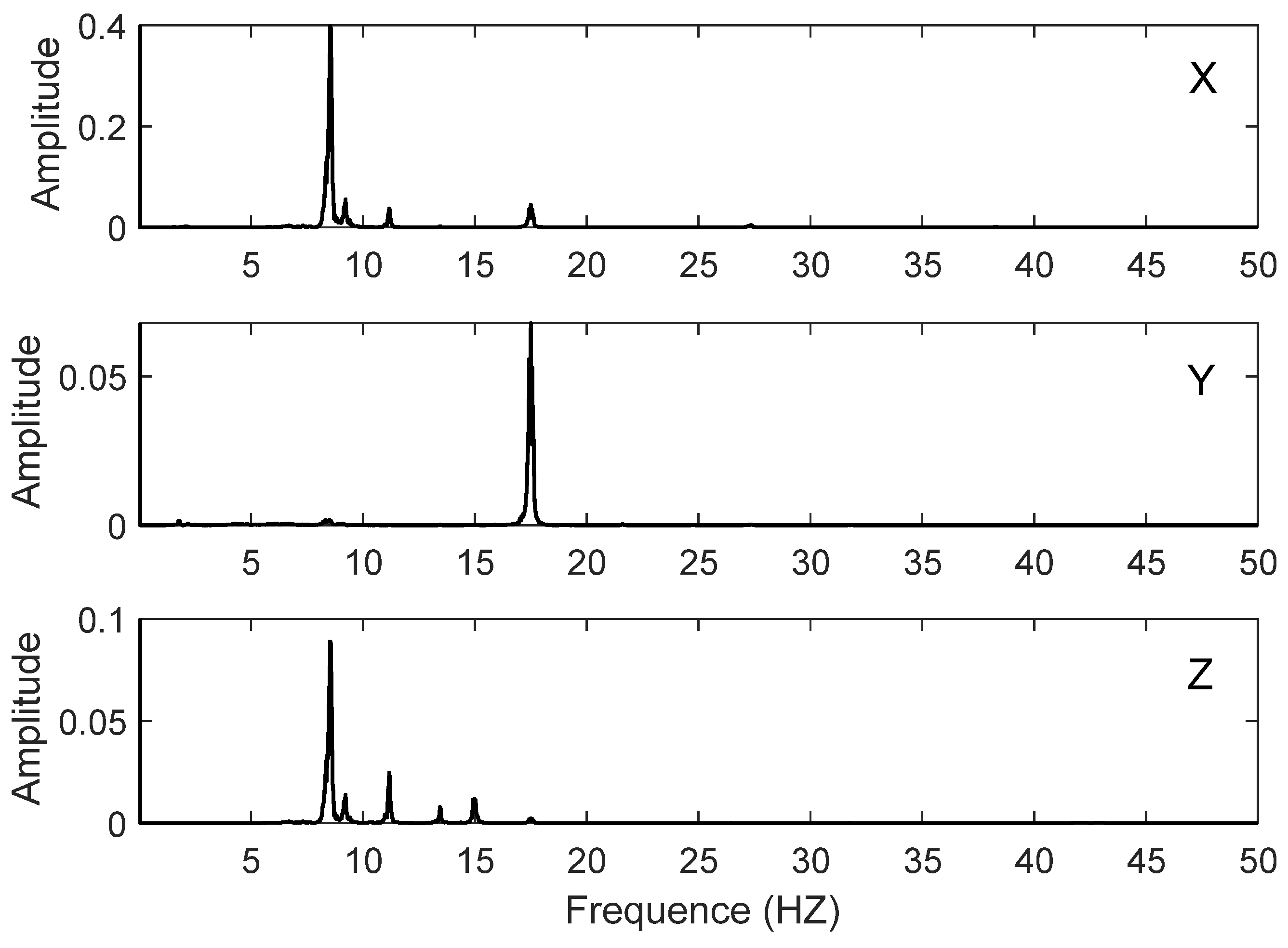
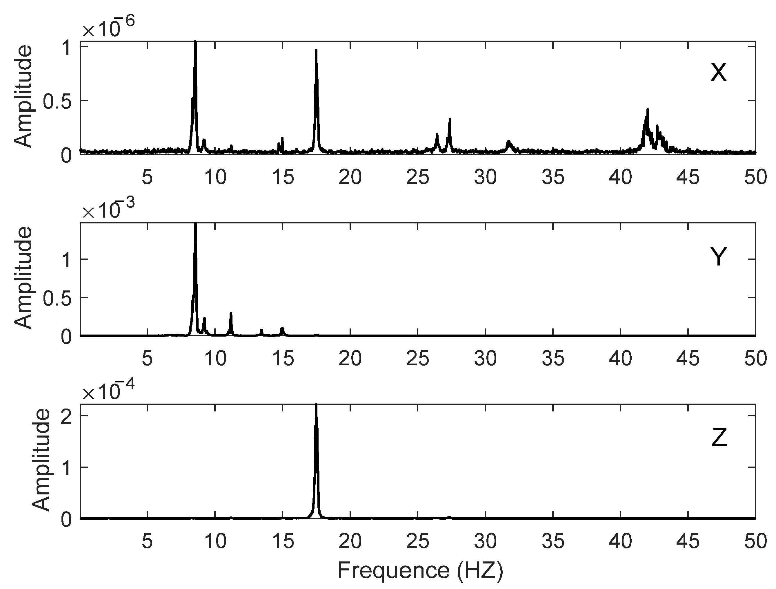
5.3. Dynamic Responses Time–Frequency Extraction

As the X-axis installation of the inertial sensor and ship collision were both directed toward the north, which means, the X-axis was the main direction of the dynamic response. Therefore, the paper only analyzed the X-axis data for dynamic response monitoring. As shown in Figure 15, the original X-axis data of the accelerometer were collected, and changes of acceleration were probably caused by multiple ship collisions; the corresponding collision time was estimated to be at the 7th s, 59th s, 89th s, 147th s, 198th s, 225th s, 237th s, and 252nd s, respectively (the second and third collisions were not obvious to be identified directly). They were basically consistent with manual records without abnormality; hence, subsequent analyses could be carried out.

PSD was utilized to extract frequencies of dynamic responses of ship collisions, as represented in the bottom of Figure 15, where four peaks can be seen at 8.55 Hz, 9.23 Hz, 11.18 Hz, and 17.50 Hz separately, with the largest peak at 8.55 Hz. It could be concluded that much information was missing in the spectrum as (i) the sequence and time of collisions were unable to be identified corresponding to the four frequencies without the time-domain information in the spectrum and (ii) only four peaks were produced by eight ship collisions, which indicated the possibility of a common frequency phenomenon or the covering of high-power spectral density on the low-power ones. Therefore, PSD could not extract complete and reliable frequencies of dynamic responses for the ship collisions.

To further study the frequency characteristics of collisions in the time domain, the VMD–HHT method proposed in this paper was adopted to carry out a three-dimensional synchronous analysis of time–frequency energy. First, five IMFs were produced using self-adaptive VMD, as illustrated in Figure 16. All those functions contained dynamic responses of ship collisions, indicating the accelerometer’s high accuracy, which was unaffected by high- and low-frequency noise and could be directly reconstructed without denoising. Later, following the Hilbert transform of the reconstructed acceleration data, the Hilbert time–frequency spectrum was obtained, as shown in Figure 11. It was evident that seven collisions, along with each corresponding time, frequency range, and energy (collision intensity), were displayed synchronously, except that the frequency range of the fifth collision was found to be between 3 Hz and 15 Hz, while others were between 5 Hz and 12 Hz. Referring to the qualitative analysis of energy, the third collision (89 s) was invisible, indicating that its intensity was the smallest. Among the seven visible collisions (Figure 17), the intensity of the second collision was the lowest, consistent with the analysis results of the original data; the intensity of the fifth collision was the highest, and its enlarged view is reflected in Figure 18, while the collision lasted for about 7 s, and the intensity changed from high to low. In summary, this VMD–HHT-based method could accurately extract frequency ranges of collisions in the time domain and clearly characterize the intensities of each collision.

5.4. Reconstruction of Dynamic Displacement Based on VMD–HHT Using Accelerometer

The frequency-domain integral equation is a powerful approach to process acceleration data using a double integral to reconstruct dynamic displacement information. According to the frequency range obtained through the VMD–HHT method, the minimum cutoff frequency was set as 1 Hz, and the maximum was set as 20 Hz. Figure 19 shows the accelerometer-derived displacement after double integration. We can observe that the displacement of the third collision (89th s) was minimal. Thus, the third collision on the platform was weak. Referring to the manual record, original data, and the HHT spectrum, the unknown displacement occurred at 180th s without any collision; the displacements of eight collisions were within 6 mm. Compared with related deformation data of bridges, high-rise buildings, and dams, deformation of the offshore oil platform collided by ships was smaller [1,9]. The reason for this is that the offshore oil platform was a stable rigid body, and the colliding ship was small when anticollision rubbers were tied to the platform pile.

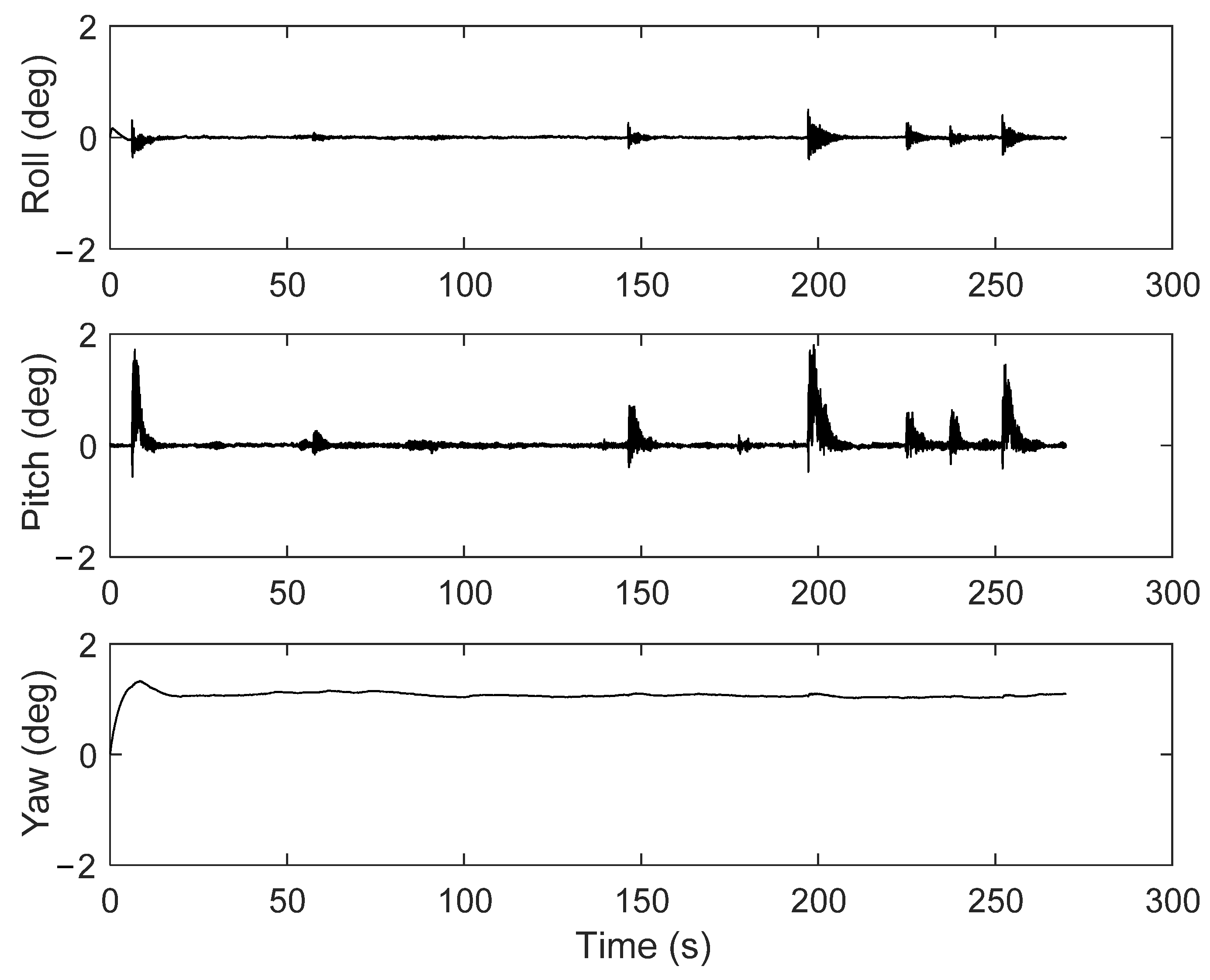
5.5. Evaluation of the Torsion Angle Based on Mahony Complementary Filter Using MIMU

To obtain torsion angle responses caused by ship collisions, the gyroscope data of MIMU were analyzed by Mahony complementary filter. Figure 20 shows the three-axis angular rate data correctly without bias, suggesting that the Y-axis of the gyroscope was influenced by the collision most. From the above analyses, it can be concluded that X-axis was the main direction of displacement response. When the ship stroked the north of the platform (X-axis), displacement responses would be caused in the same direction, while the platform was found out to incline towards Y-axis. A visual representation of the process is given in Figure 21.

Figure 22 (bottom) shows the PSD in correspondence to angular rate output in the Y-axis of the gyroscope, which included five peaks whose corresponding frequencies were 8.57 Hz, 9.23 Hz, 11.18 Hz, 13.45 Hz, and 15.00 Hz, respectively. The main peak frequency was 8.57 Hz. Referring to Figure 2, the frequencies extracted from the X-axis of the accelerometer were 8.55 Hz, 9.23 Hz, 11.18 Hz, and 17.50 Hz independently, while the main peak frequency was 8.55 Hz. By comparing two sets of data, it is evident that collision frequencies extracted from the X-axis of accelerometer and Y-axis of gyroscope were very similar. To be more specific, the distribution was consistent, but the amplitude corresponding to each frequency had a high coherence. To summarize, the frequencies of dynamic responses could be extracted from gyroscope data of MIMU.

To further explore the relationship between the accelerometer and gyroscope axis system during collisions, three-axis PSD of accelerometer and gyroscope were given, as indicated in Figure 23 and Figure 24. Amplitudes processed by PSD through accelerometer from high to low were X-axis ≥ Z-axis ≥ Y-axis. Those of gyroscope were Y-axis ≥ Z-axis ≥ X-axis, which means the event had the most significant impact on the X-axis of the accelerometer and the Y-axis of gyroscope, followed by their Z-axes. By examining the frequency distribution, the similarity of PSD was high among X-axes and Z-axes of the accelerometer and Y-axis of the gyroscope. According to the results, when the ship struck the platform from X-direction (north direction), a displacement response in the Z-axis would be caused by the displacement response of the X-axis and the rotation of the Y-axis; the PSD of the Y-axis of the accelerometer was similar to that of Z-axis of the gyroscope (as X-axis of the gyroscope was seriously affected by the noise; thus, no comparative analysis would be performed). Hereby, two conjectures are proposed as follows: (i) Since the collision direction was not completely in the X-direction and there was a component on the Y-axis, it means that a small-angle oblique impact has occurred to cause the rotation of the Z-axis, and the horizontal distortion of the platform is illustrated in Figure 25; (ii) the X-axis of the installed inertial sensor did not coincide with the north direction, that is, the installed axis deviated from the local geographical coordinate system, resulting in the component on the Y-axis to cause a small-angle oblique collision and Z-axis’ rotation.

To obtain the torsion angle response data of the platform, Mahony Complementary Filtering was used to solve the torsion angle change of platforms by integrating the information of accelerometer and gyroscope. As can be seen from the torsion angle calculation results of Figure 26, the pitch angle (Y-axis rotation) changed significantly with a maximum angle of 1.2°, followed by the roll angle (X-axis rotation) with a maximum angle of 0.15°. The heading angle (Z-axis rotation) did not change significantly with the impact event, but it deviated about 1.1° from the X direction (north direction). Therefore, Conjecture 2 could be verified. In other words, the misalignment between the installation axes of MIMU and the geographical coordinate system leads to the displacement component of the Y-axis and the rotation of the Z-axis. All the above analyses show that ship collisions will cause displacement responses and make the platform tilt or even twist. In addition, the relationship between the accelerometer and the gyroscope is also revealed: The impact on the X direction caused the Y-axis to rotate, that is, the pitch angle changes. The impact direction had a component on the Y-axis to cause the X-axis rotation, which is, the roll angle changes. The Z-axis rotation was caused by a small-angle oblique impact, which was the change of heading angle.

6. Conclusions

In this paper, a model combined by HHT and VMD is proposed to extract multidimensional dynamic responses characteristics of time, frequency, and energy of offshore oil platforms. A series of shaking-table tests and field tests in an offshore oil platform in Shengli Oilfield at Dongying City were performed using a single GPS receiver and a single accelerometer. By comparing analysis results between PSD and VMD–HHT, we found that dynamic response characteristics of ship collisions cannot be extracted entirely relying only on PSD. In contrast, VMD–HHT could effectively extract the characteristics of time, frequency, and energy simultaneously. Based on the analysis results of VMD–HHT, the dynamic displacements were reconstructed using the accelerometer in the MIMU, and the maximum displacement calculated by VMD–HHT based FDIA was 6 mm. Moreover, acceleration and angular rate obtained by MIMU had a high similarity and clear axial correlation, and such integration could also be used to calculate the torsion angle of offshore oil platforms; the maximum torsion angle is up to 1.1°.

This novel proposed method could aid in the avoidance of collisions of offshore oil platforms and be further applied in oil exploitation and platform maintenance and monitoring. However, VMD–HHT model will not be able to effectively extract feature information when the noise frequency is close to the frequency of dynamic response events.

References

1. Yang, X.F.; Wang, N. Comprehensive safety assessment method for offshore platform in different application scenarios. Energy Energy Conserv. 2021, 1, 198–200. [Google Scholar]
2. Meng, X.; Dodson, A.H.; Roberts, G.W. Detecting bridge dynamics with GPS and triaxial accelerometers. Eng. Struct. 2007, 29, 3178–3184. [Google Scholar] [CrossRef]
3. Hu, G.S. Digital Signal Processing: Theory, Algorithm and Implementation; Tsinghua University Press: Beijing, China, 2012. [Google Scholar]
4. Mateo, C.; Talavera, J. Short-time Fourier transform with the window size fixed in the frequency domain. Digit. Signal Process. 2018, 77, 13–21. [Google Scholar] [CrossRef]
5. Debnath, L.; Shah, F.A. Wavelet Transforms and Their Applications; Birkhäuser: Boston, MA, USA, 2015. [Google Scholar]
6. Wang, D.J.; Xiong, Y.L. A precise kinematic single epoch positioning algorithm using moving window wavelet denoising. Geomat. Inf. Sci. Wuhan Univ. 2015, 40, 779–785. [Google Scholar]
7. Yi, C.; Lv, Y.; Xiao, H. Multi-sensor signal denoising based on matching synchro squeezing wavelet transform for mechanical fault condition assessment. Meas. Sci. Technol. 2018, 29, 045104. [Google Scholar] [CrossRef]
8. Luo, Y.; Huang, C.; Zhang, J. Denoising method of deformation monitoring data based on variational mode decomposition. Geomat. Inf. Sci. Wuhan Univ. 2020, 45, 784–791. [Google Scholar]
9. Huang, N.E.; Shen, Z.; Long, S.R. The empirical mode decomposition and the Hilbert spectrum for nonlinear and non-stationary time series analysis. Proceedings of the Royal Society A: Mathematical. Phys. Eng. Sci. 1998, 454, 903–995. [Google Scholar] [CrossRef]
10. Chan, W.S.; Xu, Y.L.; Ding, X.L. An integrated GPS–accelerometer data processing technique for structural deformation monitoring. J. Geod. 2006, 80, 705–719. [Google Scholar] [CrossRef]
11. Barbosh, M.; Singh, P.; Sadhu, A. Empirical mode decomposition and its variants: A review with applications in structural health monitoring. Smart Mater. Struct. 2020, 29, 093001. [Google Scholar] [CrossRef]
12. Rehman, N.; Park, C.; Huang, N.E. EMD via MEMD: Multivariate noise-aided computation of standard EMD. Adv. Adapt. Data Anal. 2013, 5, 1350007. [Google Scholar] [CrossRef] [Green Version]
13. Wang, T.; Zhang, M.; Yu, Q. Comparing the applications of EMD and EEMD on time–frequency analysis of seismic signal. J. Appl. Geophys. 2012, 83, 29–34. [Google Scholar] [CrossRef]
14. Shrivastava, Y.; Singh, B. A comparative study of EMD and EEMD approaches for identifying chatter frequency in CNC turning. Eur. J. Mech. 2019, 73, 381–393. [Google Scholar] [CrossRef]
15. Yeh, J.R.; Shieh, J.S.; Huang, N.E. Complementary ensemble empirical mode decomposition: A novel noise enhanced data analysis method. Adv. Adapt. Data Anal. 2010, 2, 135–156. [Google Scholar] [CrossRef]
16. Niu, Y.; Xiong, C. Analysis of the dynamic characteristics of a suspension bridge based on RTK-GNSS measurement combining EEMD and a wavelet packet technique. Meas. Sci. Technol. 2018, 29, 85–103. [Google Scholar] [CrossRef]
17. Wang, J.; Li, Z.; Gao, J. EMD-wavelet based stochastic error reducing model for GPS/INS integrated navigation. J. Southeast Univ. 2012, 42, 406–412. [Google Scholar]
18. Song, J.G.; Zhao, C.X.; Lin, S.H. Decomposition of seismic signal based on Hilbert-Huang transform. In Proceedings of the 2011 International Conference on Business Management and Electronic Information, Guangzhou, China, 13 May 2011; pp. 840–843. [Google Scholar]
19. Zhou, Y.; Chen, W.; Gao, J. Application of Hilbert–Huang transform based instantaneous frequency to seismic reflection data. J. Appl. Geophys. 2012, 82, 68–74. [Google Scholar] [CrossRef]
20. Huang, N.E. Hilbert-Huang Transform and Its Applications, 2nd ed.; World Scientific: Singapore, 2017. [Google Scholar]
21. Shi, C.; Niu, Y.J.; Wei, N. Application of the HHT-EEMD approach in analysis of GPS height time series. J. Geod. Geodyn. 2018, 38, 661–667. [Google Scholar]
22. Mou, Z.; Niu, X.; Wang, C. A precise feature extraction method for shock wave signal with improved CEEMD-HHT. J. Ambient Intell. Humaniz. Comput. 2020, 3, 1–12. [Google Scholar] [CrossRef]
23. Luo, Y.Y.; Yao, Y.B.; Huang, C. Deformation feature extraction and analysis based on improved variational mode decomposition. Geomat. Inf. Sci. Wuhan Univ. 2020, 45, 612–619. [Google Scholar]
24. Dragomiretskiy, K.; Zosso, D. Variational mode decomposition. IEEE Trans. Signal Process. 2014, 62, 531–544. [Google Scholar] [CrossRef]
25. Wang, M.; Guan, L.; Gao, Y. UAV torsion angle measurement based on enhanced mahony complementary filter. IEEE Int. Conf. Mechatron. Autom. 2018, 545–550. [Google Scholar]
Figure 1. VMD–HHT-based characteristic extraction model.
Symmetry 13 01443 g001
Figure 2. Analog time series of acceleration.
Symmetry 13 01443 g002
Figure 3. Comparison between HHT and VMD–HHT: (a) characteristic information extraction of analog signals using HHT; (b) characteristic information extraction of analog signals using VMD–HHT.
Symmetry 13 01443 g003
Figure 4. Algorithm of frequency-domain integration.
Symmetry 13 01443 g004
Figure 5. Algorithm of Mahony complementary filtering.
Symmetry 13 01443 g005
Figure 6. Flowchart for dynamic responses based on VMD–HHT using MIMU.
Symmetry 13 01443 g006
Figure 7. Shaking table.
Symmetry 13 01443 g007
Figure 8. Instrument setup for deformation monitoring systems: (a) the layout of monitoring systems; (b) the monitoring point.
Symmetry 13 01443 g008
Figure 9. Vibration frequencies extracted by PSD.
Symmetry 13 01443 g009
Figure 10. Time–frequency–energy extracted by HHT.
Symmetry 13 01443 g010
Figure 11. Time–frequency–energy extracted by VMD–HHT.
Symmetry 13 01443 g011
Figure 12. Comparative results of vibration displacements of GNSS and FDIA.
Symmetry 13 01443 g012
Figure 13. The view of the offshore oil platform.
Symmetry 13 01443 g013
Figure 14. Instrument setup for monitoring systems of dynamic responses of offshore oil platforms: (a) the layout of monitoring systems; (b) the monitoring point of dynamic responses.
Symmetry 13 01443 g014
Figure 15. Acceleration and corresponding spectrum densities: raw signal of accelerometer (top) and power spectral density (bottom).
Symmetry 13 01443 g015
Figure 16. IMF components of accelerometer-recorded acceleration based on VMD.
Symmetry 13 01443 g016
Figure 17. HHT spectrum of acceleration.
Symmetry 13 01443 g017
Figure 18. HHT spectrum of the fifth collision.
Symmetry 13 01443 g018
Figure 19. Accelerometer-derived displacement by frequency-domain integration.
Symmetry 13 01443 g019
Figure 20. Three-axis raw signals recorded by gyroscope.
Symmetry 13 01443 g020
Figure 21. Schematic of dynamic displacement and pitch caused by the ship collision.
Symmetry 13 01443 g021
Figure 22. Gyroscope-recorded signal and corresponding spectrums: raw signal at the direction of Y (top) and power spectral density (bottom).
Symmetry 13 01443 g022
Figure 23. PSD of the acceleration recorded by the accelerometer in three directions.
Symmetry 13 01443 g023
Figure 24. PSD of the angular velocity recorded by the gyroscope in three directions.
Symmetry 13 01443 g024
Figure 25. Schematic of dynamic displacement and torsion angle caused by ship collisions.
Symmetry 13 01443 g025
Figure 26. Three-axis torsion angle by Mahony complementary filter using MIMU.
Symmetry 13 01443 g026