
Applying the Dijkstra Algorithm to Solve a Linear Diophantine Fuzzy Environment


1
Department of Mathematics, Bannari Amman Institute of Technology, Sathyamangalam 638401, Tamil Nadu, India
2
College of Vestsjaelland South & Mathematical and Physical Science Foundation, 4200 Slagelse, Denmark
3
Department of Mathematics, University of the Punjab, Lahore 54590, Pakistan
4
Department of Mathematics, College of Sciences, King Khalid University, Abha 61413, Saudi Arabia
*
Author to whom correspondence should be addressed.
Symmetry 2021, 13(9), 1616; https://0-doi-org.brum.beds.ac.uk/10.3390/sym13091616
Submission received: 28 June 2021
/
Revised: 28 July 2021
/
Accepted: 10 August 2021
/
Published: 2 September 2021
(This article belongs to the Special Issue Research on Fuzzy Logic and Mathematics with Applications)
Abstract
:Linear Diophantine fuzzy set (LDFS) theory expands Intuitionistic fuzzy set (IFS) and Pythagorean fuzzy set (PyFS) theories, widening the space of vague and uncertain information via reference parameters owing to its magnificent feature of a broad depiction area for permissible doublets. We codify the shortest path (SP) problem for linear Diophantine fuzzy graphs. Linear Diophantine fuzzy numbers (LDFNs) are used to represent the weights associated with arcs. The main goal of the presented work is to create a solution technique for directed network graphs by introducing linear Diophantine fuzzy (LDF) optimality constraints. The weights of distinct routes are calculated using an improved score function (SF) with the arc values represented by LDFNs. The conventional Dijkstra method is further modified to find the arc weights of the linear Diophantine fuzzy shortest path (LDFSP) and coterminal LDFSP based on these enhanced score functions and optimality requirements. A comparative analysis was carried out with the current approaches demonstrating the benefits of the new algorithm. Finally, to validate the possible use of the proposed technique, a small-sized telecommunication network is presented.
1. Introduction
At the heart of a network’s flow is the shortest path problem (SPP). The main challenge of an extensive range of real-life network issues is to transfer any products between two defined nodes efficiently and inexpensively. Therefore, the shortest path (SP) should then be used to formulate such real applications as discovering a route with respect to the length with the lowest cost, time, or distance from the start node (SN) to the terminal node (TN). Traditionally, it was believed that the costs traversing of edges can be represented as crisp numbers (CNs). However, since prices fluctuate with traffic patterns and weather, these values are usually imprecise or ambiguous in nature. The fuzzy set (FS) concept was introduced by Zadeh [1] to address such ambiguity. Economics, medical science research, and many other areas struggle daily with unclear, imprecise, and sometimes inadequate knowledge in ambiguous data modeling. There have been proposals for non-classical and higher-order fuzzy sets for various specialized purposes after the proposal of fuzzy set theory. Zadeh’s [1] FS theory is a valuable method for dealing with imprecise knowledge in SPPs. As a result, researchers have made numerous attempts to solve various forms of SPPs in the fuzzy domain.
Okada [2] suggested an algorithm to solve the fuzzy SPP, hinging on the possibility principle, to decide the degree of chance for each arc. Based on the fuzzy SPP, Keshavarz and Khorram [3] generalized the fuzzy SPP to a bi-level programming problem and suggested an appropriate algorithm. A constant quantity is a predicament in SPs in solving the resulting issue. With ambiguous multicriteria decision-making (MCDM) approaches focused on similarity tests, Dou et al. [4] tackled the fuzzy SP issue in a multiple constraint network. Deng et al. [5] used the ranked mean integration definition of fuzzy numbers to extend the Dijkstra algorithm to solve fuzzy SPPs. Furthermore, a few experts [6,7] have spotlighted solving the SPP in a network using heterogeneous forms of heuristic algorithm-based fuzzy arc values.
Nevertheless, FS only takes a satisfaction grade and does not convey a dissatisfaction grade. The dissatisfaction grade here is the counterpart of the satisfaction grade. The intuitionistic FS (IFS) is a generalization of FS theory, and it was introduced by Atanassov [8], who incorporated the dissatisfaction grade during the analysis. Here, the sum of the satisfaction grade and the dissatisfaction grade is less than or equal to one. In the IFS environment, some researchers are working on solving the SPP with IFS arc values. Mukherjee [9] found the SP in an IFS theory world. To address the IFS theory SPP, an alternative algorithm for the shortest path length protocol and a similarity metric for the intuitionistic fuzzy sets were proposed by Geetharamani and Jayagowri [10]. Biswas et al. [11] established a protocol for finding an intuitionist fuzzy set theory SPP between the start node (SN) and the terminal node (TN). An algorithm was developed by Kumar et al. [12] to identify the SP and the shortest distance (SD) in a network using arc weights under an interval-valued intuitionistic fuzzy set. Sujatha and Hyacinta [13] contemplated two distinct methods to solve the issue of the SP in an IFS setting. With an additional limitation under the intuitionist fuzzy setting, Motameni and Ebrahimnejad [14] focused on solving the SPP.
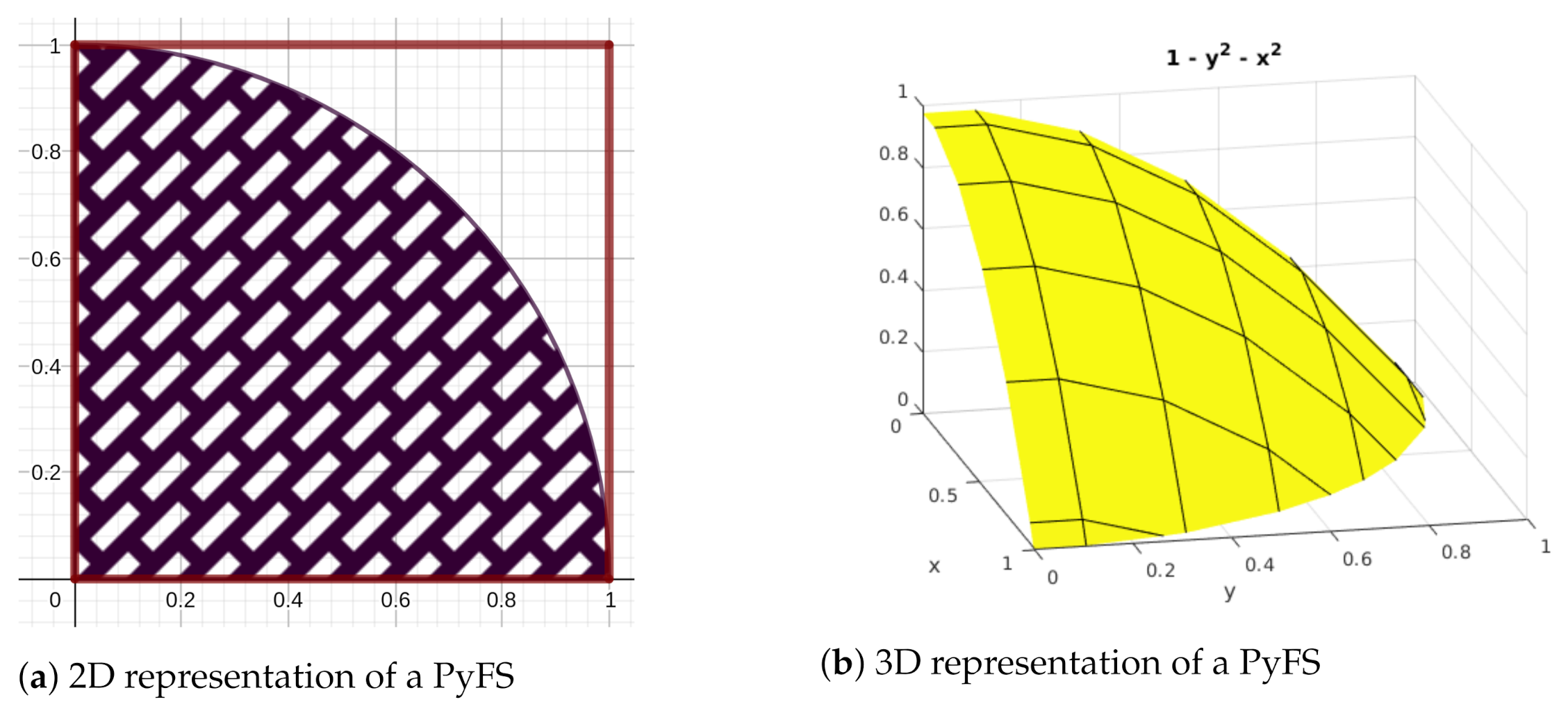
IFSs have attracted much attention and are seen in many different aspects of real life. In IFSs, the constraint sum of membership and nonmembership does not exceed one, which restricts the option to the satisfaction and dissatisfaction classes. To avoid this, Yager [15,16,17] proposed the Pythagorean fuzzy set (PyFS), which is represented by a satisfaction grade and a dissatisfaction grade with the constraint that the sum of squares of and does not exceed one. The principle of the Pythagorean fuzzy number (PyFN) was introduced by Zhang and Xu [18] to interpret the dual aspect of an element: the expert gives the details about an option with a satisfaction score of and a dissatisfaction grade of in a decision-making environment; the IFN struggles to resolve this case, as ; however, . Akram et al. [19,20] recently implemented several new Pythagorean fuzzy graph (PyFG) operations, such as exclusion, symmetric disparity, residue product, and maximal product. To extend fuzzy sets, several researchers [21,22,23,24,25,26,27,28] implemented and examined different forms of the SP algorithm.
IFSs and PyFSs have diverse applications in multiple real-life environments, but both concepts have their own limitations in the satisfaction and dissatisfaction grades. Riaz and Hashmi et al. in [29,30] presented the approach of the linear Diophantine fuzzy set (LDFS) with the inclusion of comparison parameters in order to eliminate these constraints. LDFSs are more flexible and efficient compared to the other concepts as a result of the adoption of reference parameters, which have seen a boom in recent times [31,32,33,34,35]. Recently, in 2021, Riaz et al. [30] extended their study to linear Diophantine fuzzy graph (LDFG) theory.
The SPP is the most prominent graph theory problem. For basically any fuzzy structure, it has been extensively tested (see [2,36,37,38]) with an algorithm that is relatively straightforward and gives us the best-predicted performance, as in [7], at that time. Some common methods for solving SPPs were proposed by Warshall [39], Dijkstra [40], Bellman [41], and Floyd [42]. One of the classical and best methods among them is Dijkstra’s algorithm (DA). Dijkstra’s dynamic programming (DDP) [5,43] approach may be used to solve fuzzy shortest path problems (FSPPs) by treating the weights of the edges of a network as uncertain or fuzzy. LDFSs and LDFGs are more efficient, flexible, and compatible than the existing fuzzy concepts as they have reference parameters. The research gap between these two concepts motivated us to introduce the linear Diophantine fuzzy shortest path via Dijkstra’s algorithm. This work expands the traditional Dijkstra algorithm in accordance with the aforementioned fruitful investigations, allowing us to compute the linear Diophantine fuzzy SPP’s lowest cost (LDFSPP). The LDFSPP attempts to give decision-makers the length of the LDFSP and the shortest path in a network with the linear Diophantine fuzzy arc lengths. LDFNs are assumed to be the cost parameters of the arcs. A pseudocode for this problem is provided based on Dijkstra’s techniques. Several operational requirements are described, as well as the expected LDFN values and the similarity measure LDFNs using the score and accuracy functions. Finally, a numerical example is provided to clarify the technique and demonstrate its utility and efficiency. Furthermore, our findings are compared to the current research.
The objectives of this manuscript are as follows:
- 1.
- Linear Diophantine fuzzy set (LDFS) theory is superior to intuitionistic fuzzy set (IFS), Pythagorean fuzzy set (PyFS), and q-rung orthopair fuzzy set (q-ROFS) theories, with a wide space of vague and uncertain information via reference parameters owing to its magnificent feature of a broad depiction area for permissible doublets;
- 2.
- In decision analysis, the membership and nonmembership grades are not enough to analyze objects in the universe. The addition of reference parameters provides freedom to the decision-makers in selecting the membership and nonmembership grades. The LDFS with the associated reference parameters provides a robust approach for modeling uncertainties;
- 3.
- We codify the shortest path (SP) problem for linear Diophantine fuzzy graphs;
- 4.
- Linear Diophantine fuzzy numbers are used to represent the weights associated with arcs (LDFNs);
- 5.
- The main goal of the presented work is to create a solution technique for directed network graphs by introducing linear Diophantine fuzzy (LDF) optimality constraints;
- 6.
- The weights of distinct routes are then calculated using an improved score function (SF) with the arc values represented by LDFNs;
- 7.
- The conventional Dijkstra method is further modified to find the arc weights of linear Diophantine fuzzy shortest path (LDFSP) and coterminal LDFSP based on these enhanced score functions and 11 optimality requirements;
- 8.
- A comparative analysis is carried out with the current approaches demonstrating the benefits of the new algorithm. Finally, to validate the possible use of the proposed technique, a small-sized telecommunication network is presented;
- 9.
- The suggested approach’s efficiency, rationality, and superiority are examined using a numerical example to describe the communications network; the symmetry of the optimal decision and the ranking of possible alternatives are then compared.
- 10.
- The suggested approach’s efficiency, rationality, and superiority are examined using a numerical example to describe the communications network;
- 11.
- A comparative analysis follows the symmetry of the best decision and the ranking of viable alternatives.
Therefore, this manuscript aims to suggest a technique for solving the SP problem in the LDFG context. To do so, the mathematical formulation on the SP issues is discussed first, where the traversal cost of arcs is expressed in terms of LDFNs. Then, we define the conditions of optimality in LDF networks for the solution algorithm’s design. To do so, an enhanced score feature is used to compare the costs of various routes with LDFNs representing their arc costs. The cost of the LDFSP and the corresponding LDFSP are then calculated using the standard Dijkstra algorithm. A minimal telecommunication network in the LDF setting is used to explain the proposed algorithm. The rest of the paper is organized as follows: Section 2 covers some fundamental principles of linear Diophantine fuzzy sets, while Section 3 covers the statistical formulation of the SP problem in the context of an LDF network, the LDF shortest path optimality conditions and the expanded Dijkstra algorithm. Section 4 provides a numerical example that illustrates the proposed solution methodology. The article is finally concluded in Section 5.
2. Preliminaries
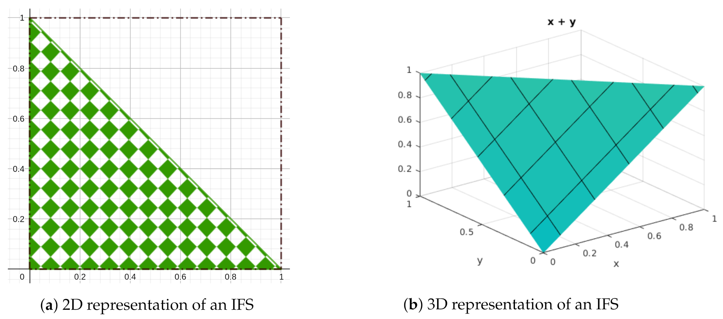
Definition 1
([8]). An IFS on the universe is defined by:
where are the satisfaction and dissatisfaction grades, respectively. The condition for an IFS is that . A doublet set is said to be an intuitionistic fuzzy number (IFN). The graphical representation of the two-dimensional (2D) and three-dimensional (3D) plots of an IFS is given in Figure 1.
Definition 2
Definition 3
([29,30]). An LDFS is an object on the nonempty reference set of the form:
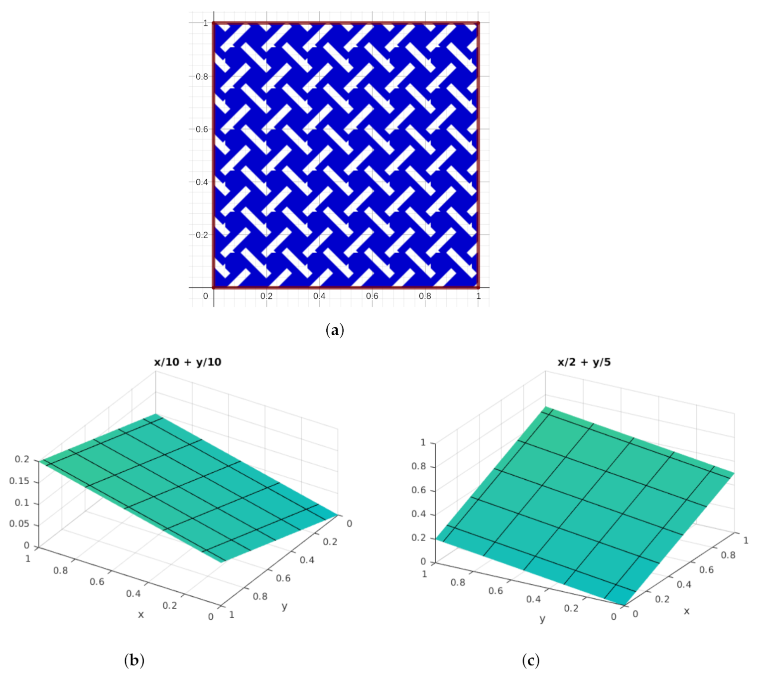
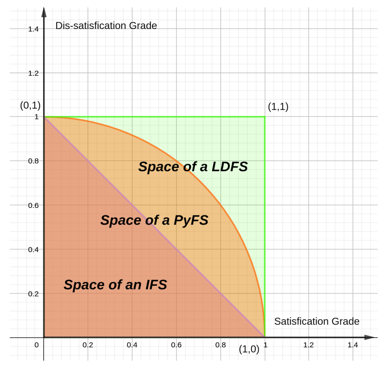
where are the satisfaction grade and dissatisfaction grade and are the reference parameters, respectively. These grades satisfy the constraint for all and with . In describing or classifying a specific system, these comparison parameters will help. By moving the physical meaning of these parameters, we can categorize the system. They expand the space used in LDFSs for grades and lift the limitations on them. The refusal grade is defined as , where γ is the refusal reference parameter. The linear Diophantine fuzzy number (LDFN) is defined as with and . The graphical representation of the 2D and 3D plots of an LDFS can be seen in Figure 3, and the comparison spaces of the IFS, PyFS, and LDFS are given in Figure 4.
Example 1.
If and , then and , but for an arbitrary choice of reference parameters with , we have . As for , we have . As a result, we managed to establish a space that is bigger than the IFS and PyFS, and we have more options to assign values to and , which is unachievable in the IFS and PyFS.
Definition 4.
An LDFS on is said to be:
- (i)
- An absolute LDFS, if it is of the form ;
- (ii)
- A null or empty LDFS, if it is of the form .
Definition 5.
Let be an LDFN, then the score function (SF) is denoted by and the accuracy function (AF) by on and can be defined by the mapping and given by:
- 1.
- 2.
where is the assembling of all LDFNs on .
Definition 6.
Let for be an assembling of LDFNs on and , then:
- (i)
- ;
- (ii)
- ;
- (iii)
- ;
- (iv)
- ;
- (v)
- ;
- (vi)
- ;
- (vii)
- ;
- (viii)
- ;
- (ix)
- .
Example 2.
Let and be two LDFNs, then:
- (i)
- ;
- (ii)
- by the Definition 6 (iii);
- (iii)
- ;
- (iv)
- ;
- (v)
- ;
- (vi)
- .If , then we have the following:
- (vii)
- ;
- (viii)
- .
Definition 7.
Two LDFNs and can be comparable using the SF and the AF. This is defined as follows:
- (i)
- if ;
- (ii)
- if ;
- (iii)
- If , then:
- (a)
- if ;
- (b)
- if ;
- (c)
- if .
Definition 8.
A pair is called an LDFG on an underlying set , where is an LDFS in and is a linear Diophantine fuzzy relation on such that:
where is known as the satisfaction grade, is known as the dissatisfaction grade, and are the reference parameters that fulfill the condition and for all , where is a linear Diophantine fuzzy vertex set and is a linear Diophantine fuzzy edge set of .
Definition 9.
A linear Diophantine fuzzy digraph or linear Diophantine fuzzy directed graph (LDFDG) with an underlying set is defined to be a pair where is an LDF set on the vertex set and is an LDF set on the edge set such that:
for all , where are the reference parameters associated with the vertex , are the reference parameters associated with the vertex , and are the reference parameters associated with the edge .
Remark 1.
As the name implies, an LDFDG does not hold a symmetric relation on , as an LDFG holds on .
3. Dijkstra Algorithm for Finding the Shortest Path in a Network
The SPP is the most prominent graph theory problem. For basically any fuzzy structure, it has been extensively tested (see [2,36,37,38])) with an algorithm that is relatively straightforward and that gives us the best-predicted performance, as in [7], at that time.
The graph is an LDF-directed graph, where and represents the vertex and edge set, respectively. The ordered pair denotes an edge of the graph that connects the two different vertices . It is considered a connected network with given arcs and nodes in which is the SN and is the TN. It is assumed that from the node to the node , there is only one directed arc. The route (path) from node to node is a series of arcs in which each arc’s initial node is the same as the corresponding arc’s terminal node in the sequence. The cost of the path that is directed is specified as the route costs the sum of the arc. The problem is to identify the SP between and for each arc-related parameter in terms of cost (or time, or space, etc.). In terms of LDFNs, this parameter is assumed to be , where is the satisfaction grade, is the dissatisfaction grade, and , are the reference parameters of the arc . This is included in the shortest path with respect to the cost for traveling along the arc .
The parameters associated with each arc reflect the expense of the arc in consideration. The objective of the SPP is to find the path or route with the lowest cost, from starting node to destination node . Certain and precise values for the arc are considered in conventional SP issues.As time and costs fluctuate regarding the payload, weather, and traffic conditions, various fuzzy set extensions may be used to reflect imprecise and ambiguous arc costs. LDFNs are used in this work to represent the ambiguous criteria of the issue of the SP under discussion. Therefore, the subsequent problem is referred to as the linear Diophantine fuzzy SP (LDFSP) problem. In an LDFSP problem with LDFNs for the arc length setting, there are two major topics that must be addressed:
- 1.
- To the linear Diophantine fuzzy arc prices, two edges are added;
- 2.
- Score functions are used to compare distance values between two distinct paths with edge lengths depicted by LDFNs.
The linear Diophantine fuzzy Dijkstra algorithm is a generalized form of the fuzzy Dijkstra’s algorithm based on its predicted values. In our next subsection, we give the linear Diophantine fuzzy Dijkstra algorithm followed by an example.
3.1. The Dijkstra Algorithm: Our Extension via the LDFG
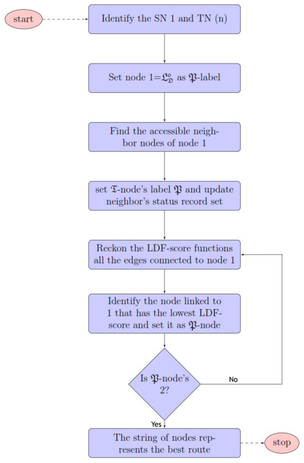
The algorithm assigns a state to each point, with the state of a node consisting of two specificities: the distance value and the status mark. A node’s “distance value” is a measurement of its source distance, and the “status mark” is a function that decides when a node’s distance value equals the shortest distance. If this is the case, the status label is permanent; otherwise, it is temporary. The algorithm incrementally preserves and updates the nodes. A single node is allocated as the current one at every stage. The pseudocode and the flowchart for the suggested process are introduced in the algorithm below and in Figure 6, respectively. Table 2 explains the set of notations used in Algorithm 1.
| Algorithm 1: Pseudo-code for the proposed linear Diophantine fuzzy Dijkstra’s algorithm (LDFDA). |
| 1. function linear Diophantine fuzzy Dijkstra’s 2. for each node //initialization 3. status label //an attribute specifying the distance value of node 4. previous not defined; //former node in optimized path from the start node 5. end for 6. status label // distance of the start node to itself 7. set of all possible nodes with temporary labels in 8. while is nonvoid // the main loop 9. node in with the minimum distance value 10. if status label 11. stop; // all the other nodes are impenetrable form the start node 12. end if 13. delete from 14. for every such that there exists link 15. //defuzzification of the linear Diophantine fuzzy number 16. if , then // comparison of the distance values values to obtain the smallest distance value 17. 18. previous 19. end if 20. status label //updated distance label 21. end for 22. end while 23. return status label []; 24. end function |
3.2. The Proposed Dijkstra Algorithm: A View
The methodology suggested in this article, in contrast to the available techniques, is more useful in finding the SP. The primary benefit of using FNs’ predicted values is that they bring out only a single value. Without the method of rating FNs, decision-making can be achieved quickly. In an area of highly ambiguous parameters, this is computationally useful for addressing SPPs. The characteristics and a comparison analysis of the four types of systems that can be used in the evaluation of SPPs are summarized in Table 3.
We claim that there are benefits to linear Diophantine fuzzy sets over ordinary FSs and IFSs, as they have a more impartial perspective of the functional situation. Therefore, our approach deals with the SPP with a network with linear Diophantine fuzzy arc lengths from the SN to the TN.
The shortest path analysis of the linear Diophantine fuzzy set is as follows:
- First of all, our approach modifies the principle of the predicted values for LDFNs. For the predicted values of LDFNs, we obtain novel results;
- We use this method of implementation to solve a well-known shortest path algorithm, the so-called Dijkstra algorithm, under which the method of the defuzzification of LDFNs allocated to network arcs is performed by computing their predicted values;
- To calculate the SD value, a juxtaposition of the LDFNs is accomplished in terms of the score function, gleaned from the predicted LDFN values, leading directly to a crisp number.
Therefore, as compared to other fuzzy shortest path methods, our accomplishment is rationally more structured, sound, and simple to add.
4. Numerical Application
It is very important to save any victims anytime a disaster happens. The urgency of time is the most salient characteristic of time-sensitive decision-making. The rescue plan must be completed within a short period, and helping the rescuers immediately know the position of any trapped persons is the job of the decision-maker. The time required to reach the rescue location almost always directly affects the performance of the rescue mission; the primary objective function is therefore considered to be the soonest achievable arrival time. When the rescue team and the police have fixed arrival times, it is possible to simplify the shortest rescue time as the shortest path desired and further as the shortest transportation time. For other factors that may present obstacles, such as damage to a bridge, the accumulation of water on a road, and damaged roads, the grade values are defined by the amount of damage to the transport infrastructure, and the weight of the path is represented by the LDFNs. This combinatorial optimization dilemma is typical of SPPs. Dijkstra’s algorithm is used to solve these types of problem. In real-time applications, a digital vector map is typically the descriptive model of an urban road network. The layout of the map related to the vertices and edges is abstracted to effectively analyze the SP. During the emergency, finding the SP to reach the destination/target is difficult. An effective deployment will boost the rescue team’s rapid response capability and total command capacity. An algorithm for the SP is developed for the directed graph, and the weights of all the edges are represented by LDFNs. Because of the unrestricted choice of attribute grades and the parameterized classification of the LDFS, this model is superior to the others. As a result, this model provides the best option for selecting an appropriate action.
The rescue location and the location of each rescue team are denoted by the vertices of the graph. The emergency team sites, passing points, and rescue points comprise a disaster area. In directed graph , denotes the location of the rescue team, the passing points, and the recovery location, and denotes the path between two rescue locations. The length of the path is important to find the minimum time to reach the rescue locations, the road conditions, etc. The edge weight is represented as an LDFN. Node , considering the geography, geographical location, the degree of the disaster’s impact, and other factors, is the beginning point of the rescue, and the point of the rescue site is node . A directed path from node to node can be represented in the form of as a series of directed edge sequences in a directed graph. Depending on the strength of the relations of a directed graph, the number of paths that connect node to node can differ.
4.1. Case Study
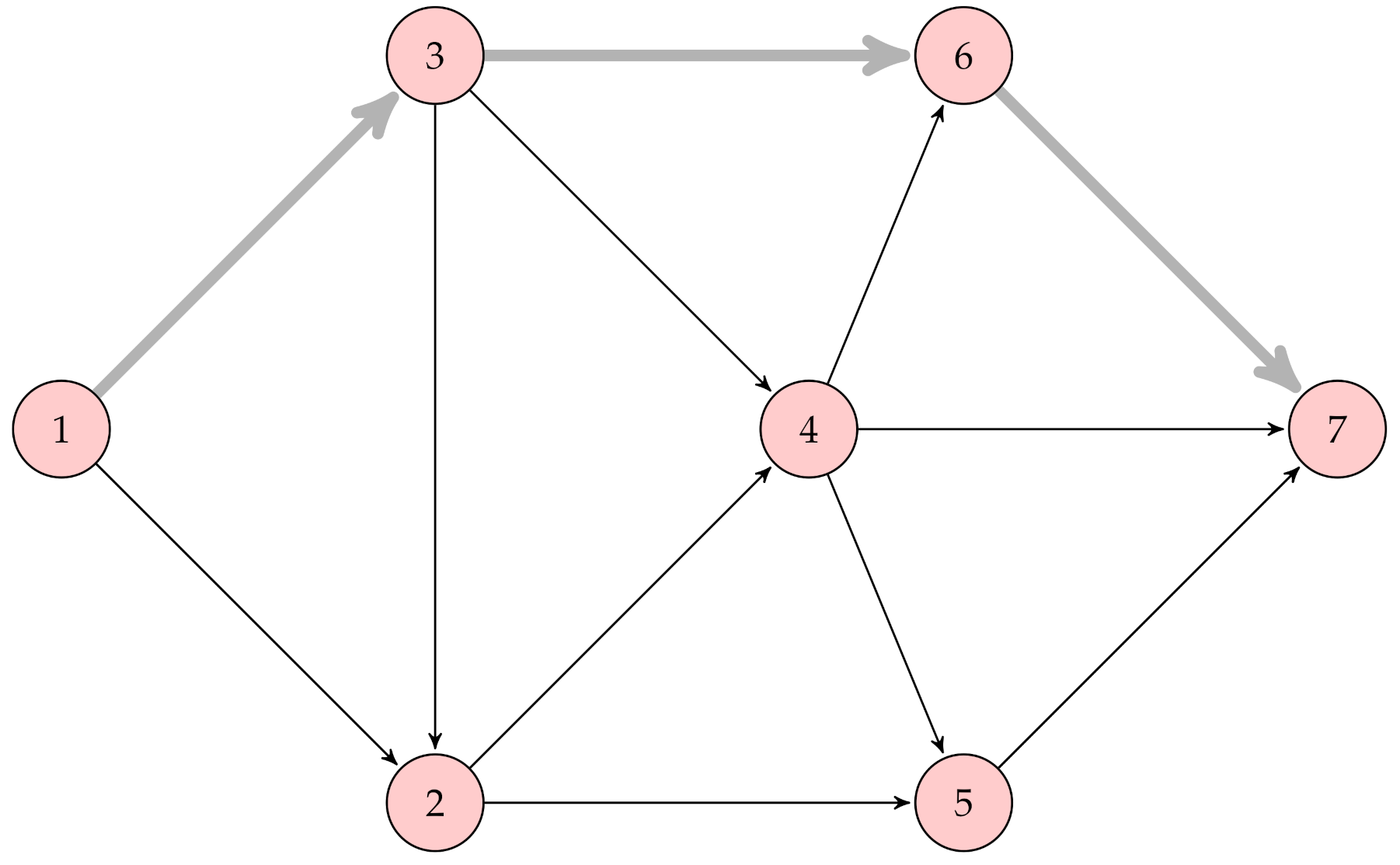
The coastal area of Wenling City, Zhejiang Province, was hit by the strong typhoon Lekima on 10 August 2019. The highest wind force was 16 levels (52 m/s), and a mean air pressure of 930 hPa was recorded at the center. Due to this strong typhoon, roads were blocked with floods, rocks, and trees, bridges were destroyed, etc. Because of this condition, it was impossible to traverse the road network based on the prior conditions. Given the road conditions, it was important to identify the safest way to the rescue point and provide the emergency rescue teams of the appropriate departments with decision-making support. During this time, the topological structure of the road network was as seen in Figure 7. We built the input data in the context of LDFSs, where the satisfaction and dissatisfaction grades informed us about the satisfaction and dissatisfaction with respect to the associated routes and their traffic signal parameters , which symbolize “very less traffic” and “very heavy traffic”. Table 4 indicates the side lengths considered. A rescue team in Fuzhou must start from Point (1) and proceed to Point (7) to rescue trapped people, so the shortest route from Point (1) to Point (7) must be identified; the sequence is illustrated below.
Let {nodes labeled as temporary nodes}, and let {nodes labeled as permanent nodes}. The start node (1) is moved from set to set at the initial point since the distance from (1) to (1) is zero, which is the shortest. The steps defined by Figure 7 to define the shortest path in the network and the SD value for all paths are defined as follows:
Let be the set of nodes labeled temporarily, and let be the set of nodes labeled permanently. The start node (1) is moved from set to set at the initial point since the distance from (1) to (1) is zero, which is the shortest:
- Iteration 0: Assign Node (1) = the permanent label = ;
- Iteration 1: We calculated the distance from the start (last permanently marked) Node (1) to its accessible neighbor Nodes (2) and (3). Consequently, the lexicon (temporary and permanent) of tagged nodes is:
Nodes Label Status 1 2 3 In order to compare , and, we used Definition 5 (1).Since the score value of is less than the score value of, the status of Node (3) is changed to permanent; - Iteration 2: Nodes (2), (4), and (6) can be accessed from the (last permanently marked) Node (3). Thus, the list (temporary and permanent) of labeled nodes becomes:
Nodes Label Status 1 2 (or) 3 4 (or) 6 (or) .Since the score value of is less than the remaining nodes,the status of Node (2) is changed to permanent; - Iteration 3: Nodes (4) and (5) can be accessed from the (last permanently marked) Node (2). Thus, the list (temporary and permanent) of labeled nodes becomes:
Nodes Label Status 1 2 3 4 (or) 5 (or) 6 (or) .Since the score value of is less than the remainingnodes, the status of Node (6) is changed to permanent; - Iteration 4: Node (7) can be accessed from the (last permanently marked) Node (6). Thus, the list (temporary and permanent) of labeled nodes becomes:
Nodes Label Status 1 2 3 4 (or) 5 (or) 6 7 (or)
(or),,.Since the score value of is less than theremaining nodes, the position of the seventh node is converted to permanent.As the point TN 7 has the permanent label, we can stop the operations at this point, and to change the remaining points as the permanent label, we have.Here, the score of is less than the score.Here, the score of is less than the score:Nodes Label Status 1 2 3 4 5 6 7
Working backward from the terminal point “7”, one can conveniently create the shortest path by moving to the predecessor from which the current node received its permanent name. Going backward, the shortest or least-expensive route becomes . Here, , the weighted aggregated LDFN of the minimum cost path or the shortest path in terms of the overall linear Diophantine fuzzy cost/time for going along the shortest path is as seen in Figure 8.
The comparative analysis of the characteristics of Dijkstra’s algorithms in the four types of systems that were used in the evaluation of SPPs are elaborated in the following Table 5.
4.2. Summary
The SPP under an LDF environment is important when the reference parameter is added to the arc weight. People and their livelihoods are affected by natural disasters in many countries such as flood, high wind force, land slides, tsunamis, etc. We considered the disaster that occurred in Wenling City, Zhejiang. Dijkstra’s algorithm was used under an LDF environment to make the right decision during an emergency. A novel Dijkstra’s algorithm was introduced and developed under an LDF setting to find the SP with the aid of the SF. The classical, fuzzy, IF, and PyF theories have their own limitations in finding the shortest paths and fail to address the reference parameters, which are important to our problem. Therefore, the LDFSPP using Dijkstra’s algorithm helped a rescue team reach the rescue destination in a short time. The proposed algorithm is more suitable for any network involving the satisfaction and dissatisfaction grades with the reference parameters.
5. Conclusions
The shortest path problem is a very important field of analysis, and it is used to solve a variety of real-world problems. In this article, a new and groundbreaking approach for solving SPPs in an unpredictable world was presented. In real-world settings, the exact cost, time, or distance values relative to the network arcs may not be possible to obtain. Fuzzy numbers can be used to describe imprecise parameters to account for this ambiguity. To reflect the unknown weights of going along each arc, the most generic kind of fuzzy numbers, LDFNs, were used. The decision-maker’s hopeful and cynical views were represented by LDFNs. The suggested technique of LDFDA was developed successfully using the LDF operator and its score functions, which are essential areas of LDFSs. SPPs with the LDF edge weight/distance have never been addressed or solved in the literature before this work. This kind of real-world problem was successfully solved using the proposed LDFDA, which successfully applied the various existing theories of LDFSs. The benefits and objectives of the paper were that the LDF optimality restrictions in directed network graphs be established and a solution method created, and then, an improved SF was used to compute the weights of alternative pathways with edge weights represented by LDFNs. To find the LDFSP and coterminal LDFSP established on these enhanced scores, the score functions and the optimality constraints of the traditional Dijkstra method were modified. Finally, to confirm the potential usage of the suggested technique, a small-scale communications network was presented, as well as a comparison study with the present approaches, proving the value of the proposed algorithm. This is the paper’s most significant contribution. Other methods for solving certain problems could be suggested in the future, and the outcomes could be compared. For large networks, computer programs may be designed to incorporate the suggested technique. In future work, we will apply the existing algorithm to solve large-scale real-time problems in a linear Diophantine fuzzy environment and compare the results with the existing algorithms with respect to the efficiency, time for computation, optimality, etc.
Author Contributions
All authors contributed equally to this paper. The individual responsibilities and contributions of all authors can be described as follows: the idea of this whole paper was put forward by M.P., M.R., S.J. and M.A. completed the preparatory work of the paper. M.R. and M.A. analyzed the existing work. The revision and submission of this paper were completed by S.J. and M.P. All authors read and agreed to the published version of the manuscript.
Funding
This research was funded by Deanship of Scientific Research at King Khalid University, Abha 61413, Saudi Arabia , grant number R.G. P-2/29/42.
Institutional Review Board Statement
Not applicable.
Informed Consent Statement
Not applicable.
Data Availability Statement
Not applicable.
Conflicts of Interest
The authors declare no conflict of interest.
Abbreviations
The following abbreviations are used in this manuscript:
| FS | fuzzy set |
| IFS | intuitionistic fuzzy set |
| PyFS | Pythagorean fuzzy set |
| LDFS | linear Diophantine fuzzy set |
| CN | crisp number |
| DA | Dijkstra’s algorithm |
| FN | fuzzy number |
| IFN | intuitionistic fuzzy number |
| PyFN | Pythagorean fuzzy number |
| LDFN | linear Diophantine fuzzy number |
| SN | start node |
| TN | terminal node |
| SP | shortest path |
| SF | score function |
| SPP | shortest path problem |
| 2D plot | two-dimensional plot |
| 3D plot | three-dimensional plot |
| SD | shortest distance |
| LDFSP | linear Diophantine fuzzy shortest path |
| MCDM | multicriteria decision-making |
References
- Zadeh, L.A. Fuzzy sets. Inf. Control 1965, 8, 338–353. [Google Scholar] [CrossRef] [Green Version]
- Okada, S.; Soper, T. A shortest path problem on a network with fuzzy arc lengths. Fuzzy Sets Syst. 2000, 109, 129–140. [Google Scholar] [CrossRef]
- Keshavarz, E.; Khorram, E. A fuzzy shortest path with the highest reliability. J. Comput. Appl. Math. 2009, 230, 204–212. [Google Scholar]
- Dou, Y.; Zhu, L.; Wang, H.S. Solving the fuzzy shortest path problem using multi-criteria decision method based on vague similarity measure. Appl. Soft Comput. 2012, 12, 1621–1631. [Google Scholar] [CrossRef]
- Deng, Y.; Chen, Y.; Zhang, Y.; Mahadevan, S. Fuzzy Dijkstra algorithm for shortest path problem under uncertain environment. Appl. Soft Comput. 2012, 12, 1231–1237. [Google Scholar] [CrossRef]
- Ebrahimnejad, A.; Karimnejad, Z.; Alrezaamiri, H. Particle swarm optimisation algorithm for solving shortest path problems with mixed fuzzy arc weights. Int. J. Appl. Decis. Sci. 2015, 8, 203–222. [Google Scholar] [CrossRef]
- Ebrahimnejad, A.; Tavana, M.; Alrezaamiri, H. A novel artificial bee colony algorithm for shortest path problems with fuzzy arc weights. Measurement 2016, 93, 48–56. [Google Scholar]
- Atanassov, K.T. Intuitionistic fuzzy sets. In Intuitionistic Fuzzy Sets; Physica: Heidelberg, Germany, 1999; pp. 1–137. [Google Scholar]
- Mukherjee, S. Dijkstra’s algorithm for solving the shortest path problem on networks under intuitionistic fuzzy environment. J. Math. Model. Algorithms 2012, 11, 345–359. [Google Scholar] [CrossRef]
- Geetharamani, G.; Jayagowri, P. Using similarity degree approach for shortest path in intuitionistic fuzzy network. In Proceedings of the 2012 International Conference on Computing, Communication and Applications, Dindigul, India, 22–24 February 2012; pp. 1–6. [Google Scholar]
- Biswas, S.S.; Alam, B.; Doja, M.N. An algorithm for extracting intuitionistic fuzzy shortest path in a graph. Appl. Comput. Intell. Soft Comput. 2013, 2013, 970197. [Google Scholar] [CrossRef] [Green Version]
- Kumar, G.; Bajaj, R.K.; Gandotra, N. Algorithm for shortest path problem in a network with interval-valued intuitionistic trapezoidal fuzzy number. Procedia Comput. Sci. 2015, 70, 123–129. [Google Scholar] [CrossRef] [Green Version]
- Sujatha, L.; Hyacinta, J.D. The shortest path problem on networks with intuitionistic fuzzy edge weights. Glob. J. Pure Appl. Math. 2017, 13, 3285–3300. [Google Scholar]
- Motameni, H.; Ebrahimnejad, A. Constraint shortest path problem in a network with intuitionistic fuzzy arc weights. In Proceedings of the International Conference on Information Processing and Management of Uncertainty in Knowledge-Based Systems, Cadiz, Spain, 11–15 June 2018; Springer: Cham, Switzerland, 2018; pp. 310–318. [Google Scholar]
- Yager, R.R. Pythagorean fuzzy subsets. In Proceedings of the 2013 Joint IFSA World Congress and NAFIPS Annual Meeting (IFSA/NAFIPS), Edmonton, AB, Canada, 24–28 June 2013; pp. 57–61. [Google Scholar]
- Yager, R.R.; Abbasov, A.M. Pythagorean membership grades, complex numbers, and decision-making. Int. J. Intell. Syst. 2013, 28, 436–452. [Google Scholar] [CrossRef]
- Yager, R.R. Pythagorean membership grades in multicriteria decision-making. IEEE Trans. Fuzzy Syst. 2013, 22, 958–965. [Google Scholar] [CrossRef]
- Zhang, X.; Xu, Z. Extension of TOPSIS to multiple criteria decision-making with Pythagorean fuzzy sets. Int. J. Intell. Syst. 2014, 29, 1061–1078. [Google Scholar] [CrossRef]
- Akram, M.; Habib, A.; Ilyas, F.; Mohsan Dar, J. Specific types of Pythagorean fuzzy graphs and application to decision-making. Math. Comput. Appl. 2018, 23, 42. [Google Scholar] [CrossRef] [Green Version]
- Akram, M.; Dar, J.M.; Naz, S. Certain graphs under Pythagorean fuzzy environment. Complex Intell. Syst. 2019, 5, 127–144. [Google Scholar] [CrossRef]
- Karthikeyan, P.; Mani, P. Applying Dijkstra Algorithm for Solving Spherical fuzzy Shortest Path Problem. Solid State Technol. 2020, 63, 4239–4250. [Google Scholar]
- Mani, P.; Vasudevan, B.; Sivaraman, M. Shortest path algorithm of a network via picture fuzzy digraphs and its application. Mater. Today Proc. 2021, 45, 3014–3018. [Google Scholar] [CrossRef]
- Parimala, M.; Broumi, S.; Prakash, K.; Topal, S. Bellman-Ford algorithm for solving shortest path problem of a network under picture fuzzy environment. Complex Intell. Syst. 2021. [Google Scholar] [CrossRef]
- Broumi, S.; Talea, M.; Bakali, A.; Smarandache, F.; Nagarajan, D.; Lathamaheswari, M.; Parimala, M. Shortest path problem in fuzzy, intuitionistic fuzzy and neutrosophic environment: An overview. Complex Intell. Syst. 2019, 5, 371–378. [Google Scholar] [CrossRef] [Green Version]
- Starczewski, J.T.; Goetzen, P.; Napoli, C. Triangular fuzzy-rough set based fuzzification of fuzzy rule-based systems. J. Artif. Intell. Soft Comput. Res. 2020, 10, 271–285. [Google Scholar] [CrossRef]
- Napoli, C.; Pappalardo, G.; Tramontana, E. A mathematical model for file fragment diffusion and a neural predictor to manage priority queues over BitTorrent. Int. J. Appl. Math. Comput. Sci. 2016, 26, 147–160. [Google Scholar] [CrossRef] [Green Version]
- Wróbel, M.; Starczewski, J.T.; Napoli, C. Grouping Handwritten Letter Strokes Using a Fuzzy Decision Tree. In Proceedings of the International Conference on Artificial Intelligence and Soft Computing, Zakopane, Poland, 12–14 October 2020; pp. 103–113. [Google Scholar]
- Fornaia, A.; Napoli, C.; Tramontana, E. Cloud services for on-demand vehicles management. Inf. Technol. Control 2017, 46, 484–498. [Google Scholar] [CrossRef] [Green Version]
- Riaz, M.; Hashmi, M.R. Linear Diophantine fuzzy set and its applications towards multi-attribute decision-making problems. J. Intell. Fuzzy Syst. 2019, 37, 5417–5439. [Google Scholar] [CrossRef]
- Riaz, M.; Hashmi, M.R.; Kalsoom, H.; Pamucar, D.; Chu, Y.M. Linear Diophantine Fuzzy Soft Rough Sets for the Selection of Sustainable Material Handling Equipment. Symmetry 2020, 12, 1215. [Google Scholar] [CrossRef]
- Ayub, S.; Shabir, M.; Riaz, M.; Aslam, M.; Chinram, R. Linear Diophantine Fuzzy Relations and Their Algebraic Properties with Decision Making. Symmetry 2021, 13, 945. [Google Scholar] [CrossRef]
- Almagrabi, A.O.; Abdullah, S.; Shams, M.; Al-Otaibi, Y.D.; Ashraf, S. A new approach to q-linear Diophantine fuzzy emergency decision support system for COVID19. J. Ambient. Intell. Humaniz. Comput. 2021. [Google Scholar] [CrossRef]
- Kamacı, H. Linear Diophantine fuzzy algebraic structures. J. Ambient. Intell. Humaniz. Comput. 2021. [Google Scholar] [CrossRef]
- Iampan, A.; García, G.S.; Riaz, M.; Athar Farid, H.M.; Chinram, R. Linear Diophantine Fuzzy Einstein Aggregation Operators for Multi-Criteria Decision-Making Problems. J. Math. 2021, 2021, 5548033. [Google Scholar] [CrossRef]
- Riaz, M.; Farid, H.M.A.; Aslam, M.; Pamucar, D.; Bozanic, D. Novel Approach for Third-Party Reverse Logistic Provider Selection Process under Linear Diophantine Fuzzy Prioritized Aggregation Operators. Symmetry 2021, 13, 1152. [Google Scholar] [CrossRef]
- Chuang, T.N.; Kung, J.Y. A new algorithm for the discrete fuzzy shortest path problem in a network. Appl. Math. Comput. 2006, 174, 660–668. [Google Scholar] [CrossRef]
- Gani, A.N.; Jabarulla, M.M. On searching intuitionistic fuzzy shortest path in a network. Appl. Math. Sci. 2010, 4, 3447–3454. [Google Scholar]
- Hernandes, F.; Lamata, M.T.; Verdegay, J.L.; Yamakami, A. The shortest path problem on networks with fuzzy parameters. Fuzzy Sets Syst. 2007, 158, 1561–1570. [Google Scholar] [CrossRef]
- Warshall, S. A theorem on boolean matrices. J. ACM 1962, 9, 11–12. [Google Scholar] [CrossRef]
- Dijkstra, E.W. A note on two problems in connexion with graphs. Numer. Math. 1959, 1, 269–271. [Google Scholar] [CrossRef] [Green Version]
- Bellman, R. On a routing problem. Q. Appl. Math. 1958, 16, 87–90. [Google Scholar] [CrossRef] [Green Version]
- Floyd, R.W. Algorithm 97: Shortest path. Commun. ACM 1962, 5, 345. [Google Scholar] [CrossRef]
- Makariye, N. Towards shortest path computation using Dijkstra algorithm. In Proceedings of the 2017 International Conference on IoT and Application (ICIOT), Nagapattinam, India, 19–20 May 2017; pp. 1–3. [Google Scholar]
- Enayattabar, M.; Ebrahimnejad, A.; Motameni, H. Dijkstra algorithm for shortest path problem under interval-valued Pythagorean fuzzy environment. Complex Intell. Syst. 2019, 5, 93–100. [Google Scholar] [CrossRef] [Green Version]
Figure 1.
Graphical representation of an IFS.

Figure 2.
Graphical representation of a PyFS.

Figure 3.
Graphical representation of an LDFS. (a) The 2D representation of an LDFS; (b) the 3D representation of an LDFS with (α, β) = (0.1, 0.1); (c) the 3D representation of an LDFS with (α, β) = (0.5, 0.2).
Figure 3.
Graphical representation of an LDFS. (a) The 2D representation of an LDFS; (b) the 3D representation of an LDFS with (α, β) = (0.1, 0.1); (c) the 3D representation of an LDFS with (α, β) = (0.5, 0.2).

Figure 4.
Spaces of the IFS, PyFS, and LDFS.

Figure 5.
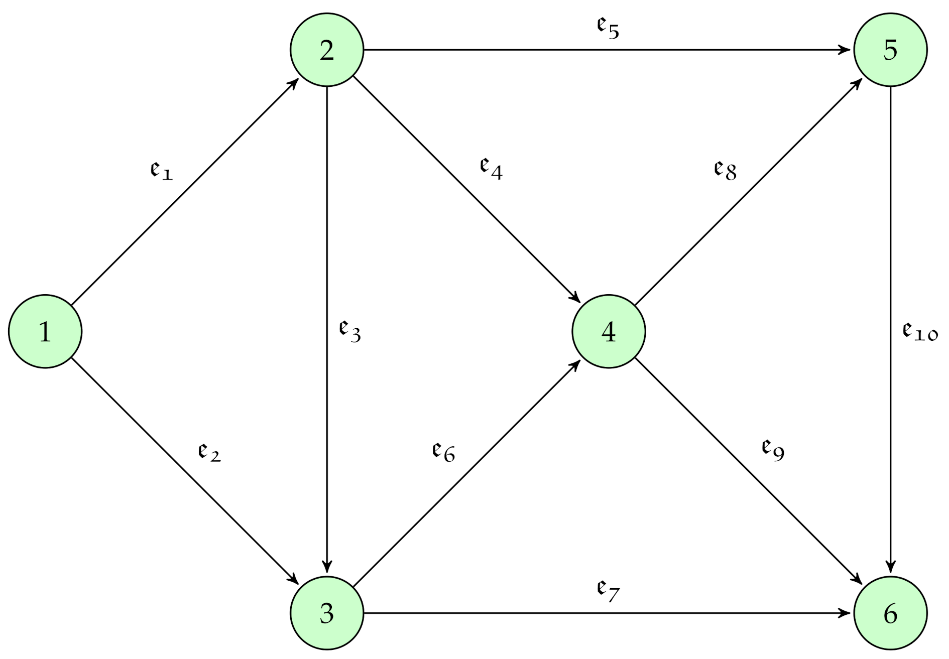
: the linear Diophantine fuzzy digraph (LDFDG).

Figure 6.
Flowchart for the proposed algorithm.

Figure 7.
The graph of the road network with the linear Diophantine fuzzy distance.

Figure 8.
Shortest path of the graph of the road network with the linear Diophantine fuzzy distance.
Figure 8.
Shortest path of the graph of the road network with the linear Diophantine fuzzy distance.


Table 1.
Index matrix of the graph .
| Vertices | ||||||
|---|---|---|---|---|---|---|
Table 2.
Notations used in the proposed Algorithm 1.
| {all temporary labeled nodes} | |
| {all permanent labeled nodes} | |
| the SD from the start node to a node | |
| a variant | |
| renovated distance from the start node | |
| cost value between nodes and | |
| alternate variant |
Table 3.
Comparison to crisp and other fuzzy models.
| SPP under Models | Links or Edges | Satisfaction Grade | Dissatisfaction Grade | Parameterization |
|---|---|---|---|---|
| Crisp set | CN | - | - | - |
| FS | FN | ✓ | - | - |
| IFS | IFN | ✓ | ✓ | - |
| PyFS | PyFN | ✓ | ✓ | - |
| LDFS | LDFN | ✓ | ✓ | ✓ |
Table 4.
Details of the edge information in terms of the LDFN.
| Edges | LDFN | Edges | LDFN |
|---|---|---|---|
| (1,2) | (3,6) | ||
| (1,3) | (4,5) | ||
| (2,4) | (4,6) | ||
| (2,5) | (4,7) | ||
| (3,2) | (5,7) | ||
| (3,4) | (6,7) |
Table 5.
Comparison analysis of Dijkstra’s algorithm under different environments.
| Types of DAs | Advantages | Limitations |
|---|---|---|
| Classical DA [40] | It can be applied when precise arc weights are available | Its performance is degradedwhen arc weights are imprecise |
| Fuzzy DA [5] | It can be applied when arc weights are imprecise | It is degradedby the degree of rejection present in the arc weight |
| IF DA [9] | It deals with imprecise arc weights involving both the degree of acceptance and the degree of rejection | It does not work if the sum of the acceptance grade and the rejection grade of an arc weight exceeds 1 |
| PyF DA [44] | It can handle imprecise arc weights even if the sum of the acceptance grade and the rejection grade exceeds 1 with some constraints | It does not work if a reference parameter is added to the arc weight |
| LDF DA (proposed method) | It can be applied in many real-time situations that ave the reference parameters | It cannot work if the indeterminacy grade is present in the arc weight |
Publisher’s Note: MDPI stays neutral with regard to jurisdictional claims in published maps and institutional affiliations. |
© 2021 by the authors. Licensee MDPI, Basel, Switzerland. This article is an open access article distributed under the terms and conditions of the Creative Commons Attribution (CC BY) license (https://creativecommons.org/licenses/by/4.0/).
Share and Cite
MDPI and ACS Style
Parimala, M.; Jafari, S.; Riaz, M.; Aslam, M. Applying the Dijkstra Algorithm to Solve a Linear Diophantine Fuzzy Environment. Symmetry 2021, 13, 1616. https://0-doi-org.brum.beds.ac.uk/10.3390/sym13091616
AMA Style
Parimala M, Jafari S, Riaz M, Aslam M. Applying the Dijkstra Algorithm to Solve a Linear Diophantine Fuzzy Environment. Symmetry. 2021; 13(9):1616. https://0-doi-org.brum.beds.ac.uk/10.3390/sym13091616
Chicago/Turabian StyleParimala, Mani, Saeid Jafari, Muhamad Riaz, and Muhammad Aslam. 2021. "Applying the Dijkstra Algorithm to Solve a Linear Diophantine Fuzzy Environment" Symmetry 13, no. 9: 1616. https://0-doi-org.brum.beds.ac.uk/10.3390/sym13091616
Note that from the first issue of 2016, this journal uses article numbers instead of page numbers. See further details here.