Study of α-Decay Energy by an Artificial Neural Network Considering Pairing and Shell Effects

Abstract

We build and train an artificial neural network (ANN) model based on experimental $\alpha$-decay energy ($Q_{\alpha }$) data. In addition to decays between the ground states of parent and daughter nuclei, decays from the ground states of parent nuclei to the excited states of daughter nuclei are also included. In this way, the number of samples is increased dramatically. The $\alpha$ particle is assumed to have a spherical symmetric shape. The root-mean-square deviation between the calculated results obtained from the ANN model and the experimental data is 0.105 MeV. It shows a good predictive power for $\alpha$-decay energy with the ANN model. The influence of different inputs is investigated. It is found that both the shell effect and the pairing effect result in an obvious improvement of the predictive power of the ANN model, and the shell effect plays a more important role. The optimal result can be obtained when both the shell and pairing effects are considered simultaneously. The application of the ANN model in predicting $\alpha$-decay energy indicates a neutron magic number at $N=184$ in the superheavy nuclei mass region.

1. Introduction

$\alpha$-decay is one of the most important decay modes of heavy nuclei. It plays a crucial role in the identification of newly synthesized superheavy elements and provides reliable information on nuclear structures. Moreover, the $\alpha$-decay half-life is one of the decisive factors for the stability of superheavy nuclei [1]. The theoretical $\alpha$-decay half-life is very sensitive to $\alpha$-decay energy which itself can reveal many nuclear structural properties [2,3,4].

$\alpha$-decay energy can be obtained from the nuclear mass difference of the involved nuclei, where nuclear mass is calculated by various theoretical mass models [5,6,7,8,9,10,11,12,13,14,15,16]. The accuracy of these mass models ranges from about 3 MeV for the Bethe–Weizsäcker (BW) model [17] to about $0.3$ MeV for the Weizsäcker–Skyrme (WS) model [9]. For heavy nuclei, an uncertainty of 1 MeV $Q_{\alpha }$ would lead to ${10}^{3-5}$ times the uncertainty of an $\alpha$-decay half-life. [18]. Such accuracy cannot meet the needs of $\alpha$-decay half-life investigation, especially for the unknown-nuclear-mass regions, such as the superheavy and neutron-rich regions. The empirical formula is also applied to investigate $\alpha$-decay energy [19,20,21,22,23]. It can be used as an effective description of $\alpha$-decay energy to some extent. Accurate descriptions of known nuclear $\alpha$-decay energy and reliable predictions of the unknown ones are indisputably required.

In recent years, machine learning has been used in the research of nuclear physics [24,25,26,27,28,29,30]. The artificial neural network is a mathematical model that mimics the function of the brain. It is composed of several processing units called neurons, which are weighted by adaptive synapses between them. It is employed to study nuclear charge radii and the ground-state energies of nuclei [24,31]. In Refs. [25,26,27,28], the Bayesian neural network (BNN) approach is used to improve the nuclear mass predictions of various models and two-neutron separation energy $S_{2n}$. It constructs a sufficiently complex neural network that can accelerate the calculation of relevant physical quantities with many parameters.

For $\alpha$-decay energy, to the best of our knowledge, except for the studies in Refs. [29,30], it is rarely investigated by using the machine learning method. In Ref. [29], $\alpha$-decay energy is calculated for the nuclei within the range $82⩽Z⩽118$ by four different machine learning models which include XGBoost, Random Forest (RF), Decision Trees (DTs), and Multilayer Perception (MLP) neural networks. It is found that XGBoost best reproduces the experimental $Q_{\alpha }$ values and the root-mean-square deviation is 0.31. In Ref. [30], the BNN model is used to calculate the $\alpha$-decay energy for the nuclei within the range $82⩽Z⩽118$. In this way, the $Q_{\alpha }$ value prediction of the Duflo–Zuker mass model has been improved and the root-mean-square deviation improvement is 72%. In both of the works, only $\alpha$-decays from the ground state of the parent nucleus to the ground state of daughter nucleus are considered.

In this work, based on experimental $\alpha$-decay energy data [32], we construct an artificial neural network to study the $Q_{\alpha }$ value. In addition to decays which involve only the ground states of the parent and daughter nuclei, the decays of the ground state of the parent nucleus to the excited state of the daughter nucleus are investigated, as well. In this way, the number of samples is increased substantially. We choose four inputs, i.e., mass number (A), proton number (Z), shell effect P, and pairing term $\delta$, to improve the accuracy of our ANN model. The trained ANN model is used to predict the $Q_{\alpha }$ for superheavy nuclei.

2. Theoretical Framework

We apply an ANN model to calculate $\alpha$-decay energy. Our model takes nuclear properties, which have important effects on the $\alpha$-decay energy of nuclei, as input and $\alpha$-decay energy $Q_{\alpha }$ as output. Such problems, where the output is a numerical value, are known as regression problems. Regression is a supervised learning problem where there is an input x and an output y, and the task is to learn the mapping from the input to the output [33]. A model in machine learning is given as below:

$$\begin{array}{c}\hfill y_{\omega ,b}\left(\mathbf{x}\right)=\varphi \left(\mathbf{xw}\right)\end{array}$$

(1)

where $\varphi$ is the activation function and $\mathit{\omega }=\left\{{\omega }_i\right\}$ are weight parameters. In our study, y corresponds to the output representing the prediction of $\alpha$-decay energy, and $\mathbf{x}=\left\{x_i\right\}$ is the input data. In the context of machine learning, the parameters ${\omega }_i$ are optimized by minimizing a loss function. Thus, the predictions are obtained as close as possible to the reference experimental data.

Multilayer perception (MLP), which is a class of feedforward artificial neural networks, is selected as the model to solve the regression problems. During the training phase of MLP, the back-propagation algorithm is used for the calculation of the gradient [34]. In recent years, a new algorithm, the adaptive gradient method called $\mathrm{Adam}$, which is a method for stochastic optimization and adapts to the learning rate of model parameters alone, was introduced and is used to train the ANN model in this paper [35,36].

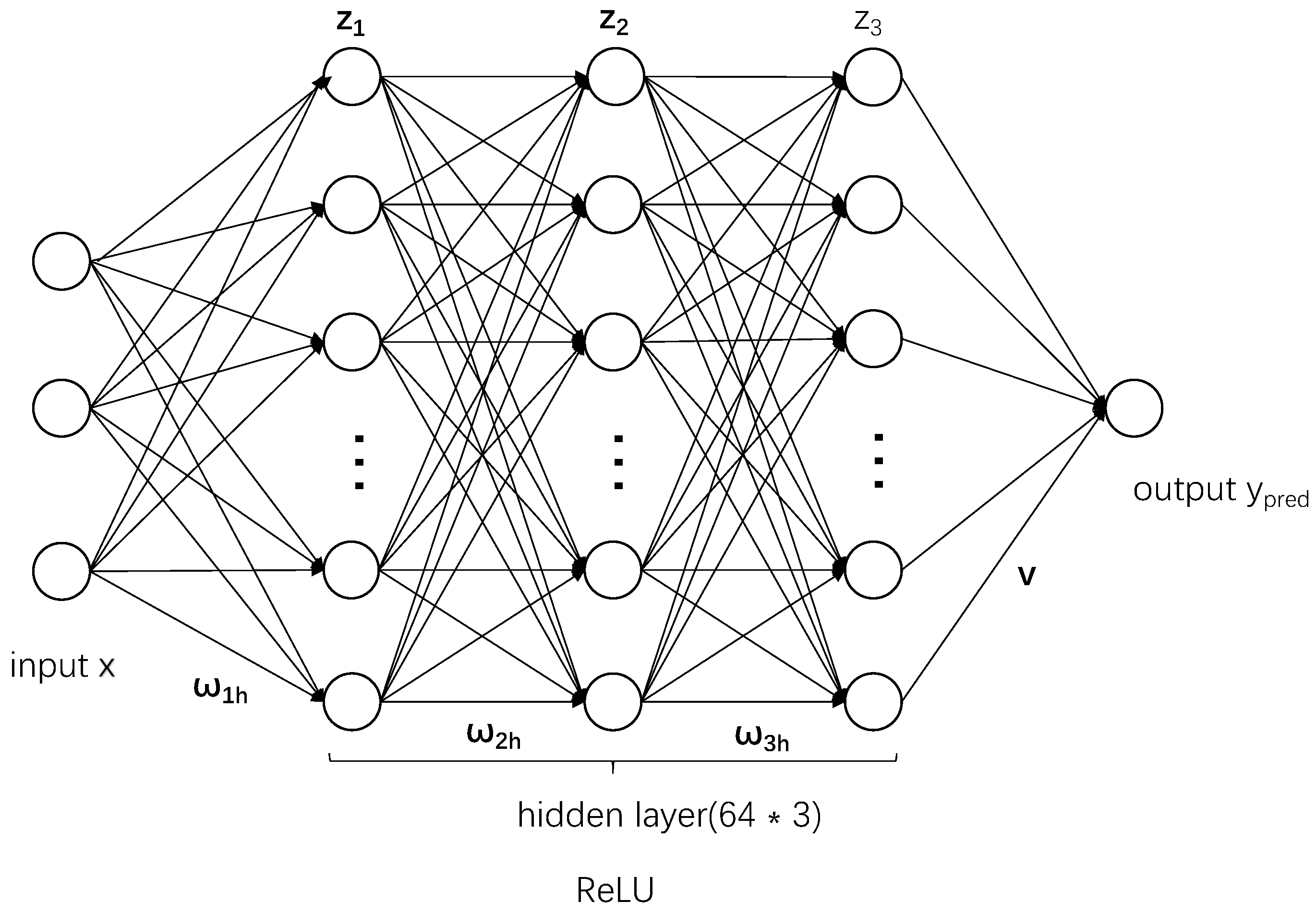
As shown in Figure 1, we implement an MLP with three hidden layers for the $\alpha$-decay energy predictions. The Rectified Linear Unit $\left(ReLU\right)$ function is chosen as the activation function with $ReLU\left(x\right)=log(1+exp(x\left)\right)$. It is close to 0 when $x_i$ is negative and close to $x_i$ when $x_i$ is positive. In Figure 1, ${\mathit{\omega }}_{1h}$, ${\mathit{\omega }}_{2h}$, and ${\mathit{\omega }}_{3h}$ are the weight parameters belonging to the first, second, and third hidden layers, respectively. The units of the first, second, and third hidden layers are expressed as ${\mathbf{z}}_{\mathbf{1}}$, ${\mathbf{z}}_{\mathbf{2}}$, and ${\mathbf{z}}_{\mathbf{3}}$, and v is the weight of the output layer. When the input x is entered into the input layer, the weighted sum is calculated and the activation is propagated forward. The $ReLU$ function is selected as activation function:

$$\begin{array}{cc}\hfill z_{ih}& =ReLU\left({\mathit{\omega }}_{ih}^T\mathit{x}\right)\hfill \\ \hfill & =ReLU(\sum _{j=1}^d{\omega }_{ihj}{x}_j),h=1,\dots ,H_i,i=1,2,3\hfill \end{array}$$

(2)

where $H_i$ is the number of neurons, ${\omega }_{ihj}$ are the weight parameters in the hidden layer i, and d is the number of characteristic quantities in the input layer. When a pattern $\mathit{x}$ appears at the input, the system calculates a response based on two rules: First, the states of all neurons within a given layer, as specified by the outputs $z_{ih}$ of Equation (2), are updated in parallel. Second, the layers are updated successively, proceeding from the input to the output layer. Therefore, the output $y_{pred}$ is computed by taking $z_3$ as input. Thus, the forward-propagation is completed.

$$y_{pred}={\mathbf{v}}^T{\mathbf{z}}_3=\sum _{h=1}^{H_3}{v}_h{z}_3+v_0$$

(3)

In our ANN model, we use 64 hidden units in each hidden layer. The prediction for $\alpha$-decay energy is a single value and only one unit exists in the output layer. The challenge of machine learning demands a learning model to perform well not only in the training set but also in the test set [37]. The results obtained from ANN are in good agreement with the experimental data. The root-mean-square deviation between calculation with the ANN model and the experimental value is very small. It is 0.09 MeV (0.135 MeV) for the training (test) data using the ANN model with four inputs. Since there is no significant difference in the root-mean-square deviation between the training set and the test set, our neural network does not overfit, even though the number of its parameters is larger than that of the training data.

The input data are randomly divided into two subsets as 80% for training and 20% for testing. The pragmatic objective of the training process will be to minimize the sum of squared errors $e_t$ relative to the experiment data. For the available experimental data $D=\left\{(x_1,y_1),(x_2,y_2),\cdots ,(x_n,y_n)\right\}$, where $x_i$ and $y_i(i=1,2,...,n)$ are input and output data and n is the number of data, the objective function is given as

$$\begin{array}{c}\hfill E(\mathbf{w},\mathbf{v}|D)=\sum _{t=1}^n{\left(e_t\right)}^2={\displaystyle \frac{{\displaystyle \sum _{t=1}^n}{(y_{pred}^t-y_{exp}^t)}^2}{n}}\end{array}$$

(4)

Here, $y_{pred}$ is the output of the ANN model, whereas $y_{exp}$ is the experimental $\alpha$-decay energy.

We use Python.Keras to build our ANN model and the Adam optimization algorithm is used to train our ANN model for 1000 epochs to minimize the mean-square error. At the same time, we require a hyperparameter called Callbacks.ReduceLROnPlateau in addition to the learning rate [38]. During training, we monitor the loss function. In the whole iteration process, when the loss function is not reduced for 100 consecutive iterations, the callbacks function is activated. Then, the gradient value in which the loss function was minimum in the previous training process is reloaded. The reloaded gradient is then reduced by a factor of 0.1, and the model continues to be optimized to find a smaller loss function.

3. Results and Discussions

3.1. Prediction of the $\alpha$-Decay Energy Based on the Experimental Data

The experimental $\alpha$-decay energies are extracted from Te ($Z=52$) to Og ($Z=118$) isotopes. The data include not only the decay from the ground state of the parent nucleus to the ground state of the daughter nucleus but also that to the exited state of the daughter nucleus. A total of 2131 $\alpha$-decay energy data are extracted.

To improve the predictive power of the ANN model, in addition to the mass (A) and proton (Z) numbers, more inputs which carry physical information should be included [28]. Thus, the inputs $\delta$ and P related to nuclear pairing and shell effects, respectively, are included. We consider these two effects separately and study their influences on the predictive performance of the ANN approach. The pairing $\delta (Z,N)$ is defined as

$$\begin{array}{c}\hfill \delta (Z,N)=[{(-1)}^Z+{(-1)}^N]/2\end{array}$$

(5)

where Z is the proton number and N is the neutron number. A positive value of the pairing term indicates a more stable nucleus, while a negative value is the opposite [17]. The shell effect P [39] reads,

$$\begin{array}{c}\hfill P={\nu }_p{\nu }_n/({\nu }_p+{\nu }_n),\end{array}$$

(6)

where ${\nu }_{p\left(n\right)}$ is the difference between the proton (neutron) numbers and the closest magic number. We take the proton and neutron magic numbers as $Z=8,20,28,50,82,126$ and $N=8,20,28,50,82,126,184$, respectively.

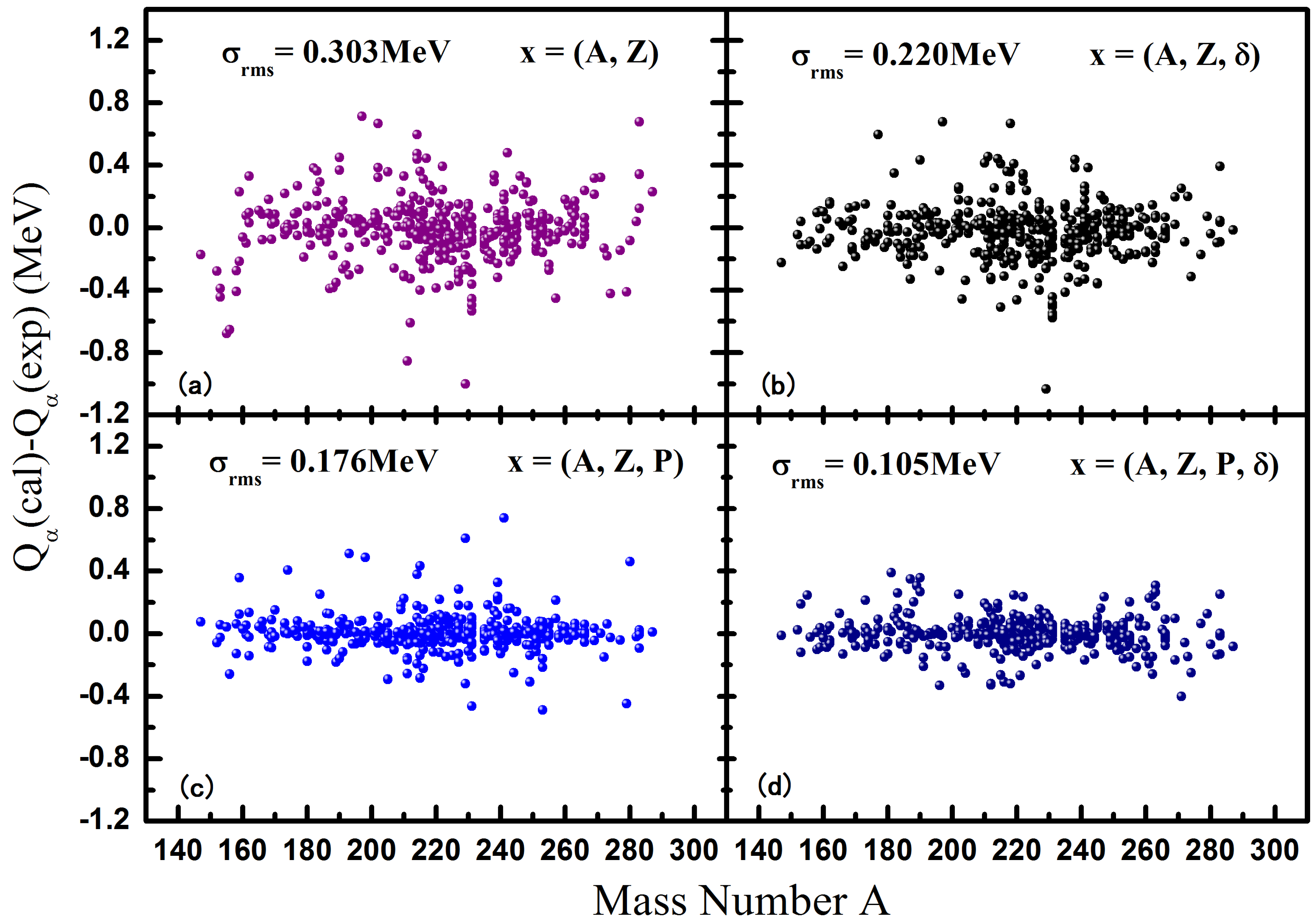
The standard deviations (in MeV) of calculated $Q_{\alpha }$ by ANN with respect to the available experiment values for different choices of input are shown in Figure 2. In Figure 2a, we consider only mass A and proton Z as inputs, and the root-mean-square is slightly higher, reaching 0.303 MeV. In order to improve the predictive power of the ANN, we add more inputs by considering the physical effects which influence the $Q_{\alpha }$ strongly. By adding pairing effect $\delta$ alone, the root-mean-square deviation is significantly reduced to 0.22 MeV. It corresponds to a $50\%$ improvement in the prediction. By adding another input shell effect P alone to the model, the root-mean-square deviation is 0.170 MeV. Compared with pairing effect $\delta$, including shell effect P improves further the accuracy of the ANN model. When we consider both the pair effect $\delta$ and the shell effect P, the root-mean-square deviation reaches a minimum value of 0.105 MeV. The results indicate that when we take appropriate physical features as inputs in the ANN model, one can obtain more accurate predictions of $\alpha$-decay energy.

The root-mean-square deviations (${\sigma }_{rms}$) of the $\alpha$-decay energy by different machine learning methods are given in

Table 1. The root-mean-square deviation (${\sigma }_{rms}$) in unit of MeV.

		ANN Model				XGBoost [29]	DZ+BNN Model [30]
input x		($A,Z$)	($A,Z$,$\delta$)	($A,Z,P$)	($A,Z,P$,$\delta$)	-	($A,Z,P$)
${\sigma }_{rms}$(MeV)	training set	0.150	0.135	0.115	0.090	-	0.178
	test set	0.303	0.220	0.176	0.105	0.403	0.274

. The present calculation exhibits relatively high predictive accuracy of the ANN model. For the test set, except for ${\sigma }_{rms}=0.303$ which is obtained with input $\mathbf{x}=(A,Z)$, all the other deviations are smaller than those given by the DZ+BNN model (${\sigma }_{rms}=0.274$) [30] and XGBoost neural network (${\sigma }_{rms}=0.310$) [29]. When input $\mathbf{x}=(A,Z,P)$ is adopted, to be the same as that used by the DZ+BNN model, ${\sigma }_{rms}=0.176$ is obtained in the ANN calculations. When further considering the pairing effect $\delta$, the result of the ANN model is improved to ${\sigma }_{rms}=0.105$. This shows a relatively high predictive power. Since the most powerful prediction is given by using the input $\mathbf{x}=(Z,A,\delta ,P)$, the following calculations used to discuss the $\alpha$-decay energy in the SHE region are all calculated by using the input $\mathbf{x}=(Z,A,\delta ,P)$.

Note that the above comparisons based on the assessment of root-mean-square deviations are only performed on different inputs. In the present work, we extract the $\alpha$-decay energy $Q_{\alpha }$ from the ground state of the parent nucleus to the ground state of the daughter and also to the excited state of the daughter nucleus. Therefore, the amount of sample data is increased, which can improve the predictive power of the ANN model. The influence of other factors, such as data size, symmetry energy, and so on, on the root-mean-square deviations of the different models needs further investigation.

3.2. Extrapolation of the $\alpha$-Decay Energy in the Superheavy Nuclei Mass Region

In the superheavy nuclei mass region where there are no sufficient experimental data available, the accurate predictions of the $\alpha$-decay energy and the half-lives of $\alpha$-decay are very important, both for the synthesis of new superheavy elements and the structural study of superheavy nuclei. From the above discussion, one can see that the ANN model has a relatively high predictive power for $\alpha$-decay energy. We apply the above ANN approach to calculate the $\alpha$-decay energy of radionuclides in the SHE region. The comparison of the $\alpha$-decay energies calculated by the ANN model with the experimental data for $104⩽Z⩽118$ are listed in

Table 2. The comparison of the $\alpha$-decay energies calculated by the ANN model with the experimental data for $104⩽Z⩽118$. The first four columns denote the parent nucleus, its mass number, experimental and predicted $\alpha$-decay energy (in MeV), respectively. The last column is the root-mean-square deviation (in MeV) for each element.

Parent Nuclei	${\mathit{A}}_{\mathit{p}}$	${\mathit{Q}}^{\mathbf{exp}}$ (MeV)	${\mathit{Q}}^{\mathbf{pred}}$ (MeV)	${\mathit{\delta }}_{\mathbf{rms}}$ (MeV)	Parent Nuclei	${\mathit{A}}_{\mathit{p}}$	${\mathit{Q}}^{\mathbf{exp}}$ (MeV)	${\mathit{Q}}^{\mathbf{pred}}$ (MeV)	${\mathit{\delta }}_{\mathbf{rms}}$ (MeV)
${}_{104}$Rf	255	9.055	9.065		${}_{105}$Db	270	9.265	9.458
${}_{104}$Rf	256	8.926	8.955		${}_{105}$Db	263	9.206	9.057
${}_{104}$Rf	257	9.083	9.065		${}_{105}$Db	262	9.501	9.620
${}_{104}$Rf	258	9.193	9.588		${}_{105}$Db	257	9.620	9.507
${}_{104}$Rf	259	9.131	9.242		${}_{105}$Db	261	9.500	9.302
${}_{104}$Rf	261	8.648	8.758	0.173	${}_{105}$Db	256	9.218	9.163
${}_{106}$Sg	271	9.821	9.815		${}_{105}$Db	260	9.050	8.960
${}_{106}$Sg	269	9.901	9.861		${}_{105}$Db	258	8.834	8.808
${}_{106}$Sg	266	9.714	9.546		${}_{105}$Db	259	8.020	7.928	0.127
${}_{106}$Sg	263	9.403	9.333		${}_{107}$Bh	274	10.401	10.367
${}_{106}$Sg	261	8.763	8.721		${}_{107}$Bh	270	10.503	10.278
${}_{106}$Sg	259	8.631	8.552		${}_{107}$Bh	272	10.319	10.076
${}_{106}$Sg	260	8.561	8.202	0.156	${}_{107}$Bh	266	9.967	9.781
${}_{108}$Hs	270	11.059	10.872		${}_{107}$Bh	264	9.550	9.496
${}_{108}$Hs	269	10.591	10.539		${}_{107}$Bh	262	9.061	9.344
${}_{108}$Hs	275	10.586	10.528		${}_{107}$Bh	260	9.301	9.228
${}_{108}$Hs	273	10.335	10.162		${}_{107}$Bh	261	8.951	8.795	0.179
${}_{108}$Hs	267	10.110	10.148		${}_{109}$Mt	278	11.480	11.284
${}_{108}$Hs	266	9.315	9.790		${}_{109}$Mt	276	10.695	10.971
${}_{108}$Hs	265	9.070	9.256		${}_{109}$Mt	270	10.181	10.774
${}_{108}$Hs	264	9.670	9.428		${}_{109}$Mt	275	10.600	10.488
${}_{108}$Hs	263	9.440	9.110	0.235	${}_{109}$Mt	274	10.481	10.021
${}_{110}$Ds	281	11.780	11.692		${}_{109}$Mt	268	10.101	10.049
${}_{110}$Ds	279	11.680	11.336		${}_{109}$Mt	266	9.631	9.581	0.315
${}_{110}$Ds	277	11.117	11.022		${}_{111}$Rg	282	11.197	11.648
${}_{110}$Ds	271	10.899	11.029		${}_{111}$Rg	281	11.481	11.435
${}_{110}$Ds	270	11.371	10.879		${}_{111}$Rg	280	10.851	10.797
${}_{110}$Ds	273	10.710	10.282		${}_{111}$Rg	279	10.520	10.461
${}_{110}$Ds	269	9.840	9.833		${}_{111}$Rg	278	10.147	10.139
${}_{110}$Ds	267	8.853	9.158	0.289	${}_{111}$Rg	272	9.415	9.664
${}_{112}$Cn	285	11.595	11.388		${}_{111}$Rg	274	9.160	9.652	0.271
${}_{112}$Cn	283	10.450	10.160		${}_{113}$Nh	285	11.851	11.775
${}_{112}$Cn	281	9.761	9.778		${}_{113}$Nh	286	10.781	10.583
${}_{112}$Cn	277	9.291	9.367	0.182	${}_{113}$Nh	283	10.261	10.192
${}_{114}$Fl	289	10.561	10.295		${}_{113}$Nh	284	10.281	10.251
${}_{114}$Fl	288	10.370	10.230		${}_{113}$Nh	282	9.615	9.851
${}_{114}$Fl	287	10.161	10.059		${}_{113}$Nh	278	9.791	9.765	0.133
${}_{114}$Fl	286	10.072	10.089		${}_{115}$Mc	290	10.471	10.477
${}_{114}$Fl	285	9.961	9.963	0.141	${}_{115}$Mc	289	10.751	10.579
${}_{116}$Lv	293	11.001	10.954		${}_{115}$Mc	287	10.456	10.387
${}_{116}$Lv	292	10.891	10.714		${}_{115}$Mc	288	10.451	10.441	0.092
${}_{116}$Lv	291	10.774	10.802		${}_{117}$Ts	293	11.184	11.061
${}_{116}$Lv	290	10.671	10.616	0.095	${}_{117}$Ts	294	11.201	11.113	0.106
${}_{118}$Og	294	11.861	11.697	0.164	all nuclei				0.204

. The first four columns denote the parent nucleus, its mass number, and experimental and predicted $\alpha$-decay energy, respectively. The last column is the root-mean-square deviation for each element. The root-mean-square deviation of all $\alpha$-decay energies calculated in the SHE region is 0.204 MeV. The corresponding root-mean-square deviation for each element is below 0.320 MeV, which is comparable to the results obtained by the theoretical studies in Refs. [22,40]. The element with the largest root-mean-square deviation is the Mt isotope (${\sigma }_{rms}=0.315$ MeV). The uncertainty of the $\alpha$-decay energy $Q_{\alpha }$ leads to ${10}^{1-2}$ times the uncertainty of the $\alpha$-decay half-life. It confirms to us that the ANN model can give a good prediction of the $Q_{\alpha }$ values in the SHE region. However, the decay of the SHE is very complicated. Besides $\alpha$-decay, other decay modes such as spontaneous fission play very important roles, which needs further investigation in the future.

The detailed comparison of the calculated $Q_{\alpha }$ with the available experimental data for the $Z=104-118$ isotope chains is shown in Figure 3, in which the results are divided into four groups. The neutron numbers vary from $N=151$ to 189. The calculated ANN results are denoted by solid lines and the experimental data by solid circles. One can see that the experimental data are reproduced well by the ANN model. The local minimum of the $Q_{\alpha }$ curves with the neutron number N of the parent nucleus could indicate a shell gap. The dashed vertical lines mark the neutron numbers, at which there are possible existent shell gaps.

As shown in Figure 3, a clear local minimum appears at $N=184$ for almost all the $Z=104-118$ isotope chains, which indicates a big shell gap. For $Z=118$, the minimum of $Q_{\alpha }$ is predicted at N = 183 instead of 184. This is partly because there are few experimental data for Og isotopes in the training model. As we know, the prediction of the next closed shell beyond ${}^{208}$Pb is the critical point in synthesizing superheavy elements. Different theoretical models usually predict different closed shells. In the present work, based on the training of the ANN model by the experimental $Q_{\alpha }$, a big shell gap effect is predicted at $N=184$, which is consistent with the predicted neutron magic number by theoretical nuclear models in the literature [41,42,43].

4. Summary

We build and train an ANN model by extracting experimental $Q_{\alpha }$ values from the ground states of parent nuclei to the ground and excited states of daughter nuclei. In this way, the number of samples increases substantially. The ANN model is trained to have stronger prediction power. To obtain a high predictive power, besides mass number A and proton number Z, two more inputs, i.e., P and $\delta$, which are related to nuclear shell effect and pair effect, respectively, are considered. By studying 2131 $\alpha$-decays, the root-mean-square deviation of the $\alpha$-decay energy is 0.105 MeV, which presents great accuracy. In addition, the influence of different inputs on predictive power is investigated. It is found that considering both the shell effect and the pairing effect leads to an obvious improvement of the result and that the shell effect plays a more important role. The optimal result is obtained when both the shell and pairing effects are considered simultaneously. The ANN model is used to study the $\alpha$-decay energies in superheavy nuclear mass regions where experimental data are rare. A clear minimum of the predicted $Q_{\alpha }$ at $N=184$ by the ANN model indicates a big shell gap for nuclei in the SHE region, which is consistent with the prediction of a neutron magic number at $N=184$ by theoretical nuclear models.

References

- Hofmannand, S.; Munzenberg, G. The discovery of the heaviest elements. Rev. Mod. Phys. 2000, 72, 733–767. [Google Scholar] [CrossRef]
- Ren, Z.Z.; Xu, G.G. Reduced alpha transfer rates in a schematic model. Phys. Rev. C 1987, 36, 456–459. [Google Scholar] [CrossRef]
- Hodgson, P.E.; Běták, E. Cluster emission, transfer and capture in nuclear reactions. Phys. Rep. 2003, 374, 1–89. [Google Scholar] [CrossRef]
- Seweryniak, D.; Starosta, K.; Davids, C.N.; Gros, S.; Hecht, A.A.; Hoteling, N.; Khoo, T.L.; Lagergren, K.; Lotay, G.; Peterson, D.; et al. α decay of 105Te. Phys. Rev. C 2006, 73, 061301. [Google Scholar] [CrossRef]
- Duflo, J.; Zuker, A.P. Microscopic mass formulas. Phys. Rev. C 1995, 52, R23–R27. [Google Scholar] [CrossRef] [Green Version]
- Vogt, K.; Hartmann, T.; Zilges, A. Simple parametrization of single- and two-nucleon separation energies in terms of the neutron to proton ratio N/Z. Phys. Lett. B 2001, 517, 255–260. [Google Scholar] [CrossRef] [Green Version]
- Bethe, H.A.; Bacher, R.F. Nuclear Physics A. Stationary States of Nuclei. Rev. Mod. Phys. 1936, 8, 82–229. [Google Scholar] [CrossRef] [Green Version]
- Möller, P.; Myers, W.D.; Sagawa, H.; Yoshida, S. New Finite-Range Droplet Mass Model and Equation-of-State Parameters. Phys. Rev. Lett. 2012, 108, 052501. [Google Scholar] [CrossRef] [Green Version]
- Wang, N.; Liu, M.; Wu, X.; Meng, J. Surface diffuseness correction in global mass formula. Phys. Lett. B 2014, 734, 215–219. [Google Scholar] [CrossRef] [Green Version]
- Goriely, S.; Chamel, N.; Pearson, J.M. Skyrme-Hartree-Fock-Bogoliubov Nuclear Mass Formulas: Crossing the 0.6 MeV Accuracy Threshold with Microscopically Deduced Pairing. Phys. Rev. Lett. 2009, 102, 152503. [Google Scholar] [CrossRef] [Green Version]
- Goriely, S.; Chamel, N.; Pearson, J.M. Further explorations of Skyrme-Hartree-Fock-Bogoliubov mass formulas. XVI. Inclusion of self-energy effects in pairing. Phys. Rev. C 2016, 93, 034337. [Google Scholar] [CrossRef]
- Von-Eiff, D.; Freyer, H.; Stocker, W.; Weigel, M.K. The relativistic spin-orbit force near the neutron-drip line. Phys. Lett. B 1995, 344, 11–17. [Google Scholar] [CrossRef]
- Vretenar, D.; Afanasjev, A.V.; Lalazissis, G.A.; Ring, P. Relativistic Hartree-Bogoliubov theory: Static and dynamic aspects of exotic nuclear structure. Phys. Rep. 2005, 409, 101–259. [Google Scholar] [CrossRef]
- Meng, J.; Peng, J.; Zhang, S.Q.; Zhou, S.G. Possible existence of multiple chiral doublets in 106Rh. Phys. Rev. C 2006, 73, 037303. [Google Scholar] [CrossRef] [Green Version]
- L, H.Z.; Giai, N.V.; Meng, J. Spin-Isospin Resonances: A Self-Consistent Covariant Description. Phys. Rev. Lett. 2008, 101, 122502. [Google Scholar] [CrossRef] [Green Version]
- Niu, Z.M.; Niu, Y.F.; Liang, H.Z.; Long, W.H.; Meng, J. Self-consistent relativistic quasiparticle random-phase approximation and its applications to charge-exchange excitations. Phys. Rev. C 2017, 95, 044301. [Google Scholar] [CrossRef] [Green Version]
- Kirson, M.W. Mutual influence of terms in a semi-empirical mass formula. Nucl. Phys. A 2008, 798, 29–60. [Google Scholar] [CrossRef]
- Möller, P.; Nix, J.R.; Kratz, K.L. Nuclear Properties for Astrophysical and Radioactive-Ion-Beam Applications. At. Data Nucl. Data Tables 1997, 66, 131–343. [Google Scholar] [CrossRef] [Green Version]
- Jia, J.H.; Qian, Y.B.; Ren, Z.Z. Systematics of α-decay energies in the valence correlation scheme. Phys. Rev. C 2021, 103, 024314. [Google Scholar] [CrossRef]
- Dong, T.; Ren, Z.Z. α-decay energy formula for superheavy nuclei based on the liquid-drop model. Phys. Rev. C 2010, 82, 034320. [Google Scholar] [CrossRef]
- Ni, D.D.; Ren, Z.Z. Binding energies, α-decay energies, and α-decay half-lives for heavy and superheavy nuclei. Nucl. Phys. A 2012, 893, 13–26. [Google Scholar] [CrossRef]
- Jiang, H.; Fu, G.J.; Sun, B.; Liu, M.; Wang, N.; Wang, M.; Ma, Y.G.; Lin, C.J.; Zhao, Y.M.; Zhang, Y.H.; et al. Predictions of unknown masses and their applications. Phys. Rev. C 2012, 85, 054303. [Google Scholar] [CrossRef]
- Dong, J.; Wei, Z.; Scheid, W. Correlation between alpha-decay Energies of Superheavy Nuclei Involving Effect of Symmetry Energy. Phys. Rev. Lett. 2011, 107, 012501. [Google Scholar] [CrossRef] [PubMed] [Green Version]
- Hao, X.; Zhang, G.; Ma, S. Deep learning; World Scientific: Singapore, 2016; Volume 10, pp. 417–439. [Google Scholar]
- Niu, Z.M.; Liang, H.Z. Nuclear mass predictions based on Bayesian neural network approach with pairing and shell effects. Phys. Lett. B 2018, 778. [Google Scholar] [CrossRef]
- Neufcourt, L.; Cao, Y.; Nazarewicz, W.; Viens, F. Bayesian approach to model-based extrapolation of nuclear observables. Phys. Rev. C 2018, 98, 034318. [Google Scholar] [CrossRef] [Green Version]
- Neufcourt, L.; Cao, Y.; Nazarewicz, W.; Olsen, E.; Viens, F. Neutron Drip Line in the Ca Region from Bayesian Model Averaging. Phys. Rev. Lett. 2019, 122, 062502.1–062502.6. [Google Scholar] [CrossRef] [Green Version]
- Yüksel, E.; Soydaner, D.; Bahtiyar, H. Nuclear mass predictions using neural networks: Application of the multilayer perceptron. Int. J. Mod. Phys. E 2021, 30. [Google Scholar] [CrossRef]
- Saxena, G.; Sharma, P.K.; Saxena, P. Modified empirical formulas and machine learning for α-decay systematics. J. Phys. G Nucl. Part. Phys. 2021, 48, 055103. [Google Scholar] [CrossRef]
- Rodríguez, U.B.; Vargas, C.Z.; Gonçalves, M.G.; Barbosa, S.D.; Guzman, F. Alpha half-lives calculation of superheavy nuclei with Qα-values predictions based on Bayesian neural network approach. J. Phys. G Nucl. Part. Phys. 2019, 46, 115109. [Google Scholar] [CrossRef]
- Akkoyun, S.; Bayram, T.; Kara, S.O.; Sinan, A. An artificial neural network application on nuclear charge radii. J. Phys. G Nucl. Part. Phys. 2013, 40, 055106-1–055106-7. [Google Scholar] [CrossRef]
- Available online: https://www.nndc.bnl.gov/ensdf/ (accessed on 25 March 2022).
- Dnmez, P. Introduction to Machine Learning, 2nd ed.; Alpaydn, E., Ed.; The MIT Press: Cambridge, MA, USA, 2010. [Google Scholar]
- Rumelhart, D.; Hinton, G.E.; Williams, R.J. Learning Representations by Back Propagating Errors. Nature 1986, 323, 533–536. [Google Scholar] [CrossRef]
- Lecun, Y.; Bengio, Y.; Hinton, G. Deep learning. Nature 2015, 521, 436. [Google Scholar] [CrossRef] [PubMed]
- Schmidhuber, J. Deep learning in neural networks: An overview. Neural Netw. 2015, 61, 85–117. [Google Scholar] [CrossRef] [PubMed] [Green Version]
- Jeff, H. Ian Goodfellow, Yoshua Bengio, and Aaron Courville: Deep learning. In Genetic Programming and Evolvable Machines; Springer: Berlin, Germany, 2017; pp. 1–3. [Google Scholar]
- Htike, K.K.; Hogg, D. Unsupervised detector adaptation by joint dataset feature learning. In Proceedings of the International Conference on Computer Vision and Graphics, Warsaw, Poland, 15–17 September 2014; pp. 270–277. [Google Scholar]
- Kortelainen, M.; Mcdonnell, J.; Nazarewicz, W.; Reinhard, P.G.; Sarich, J.; Schunck, N.; Stoitsov, M.V.; Wild, S.M. Nuclear energy density optimization: Large deformations. Phys. Rev. C 2011, 85, 024304. [Google Scholar] [CrossRef]
- Qian, Y.B.; Ren, Z.Z. Robustness of heavy and superheavy nuclei against α decay: Progress toward identifying the possible location of the “island of stability”. Phys. Rev. C 2019, 100, 061302. [Google Scholar] [CrossRef]
- Nilsson, S.; Nix, J.; Sobiczewski, A.; Szymański, Z.; Wycech, S.; Gustafson, C.; Möller, P. On the spontaneous fission of nuclei with Z near 114 and N near 184. Nucl. Phys. A 1968, 115, 545–562. [Google Scholar] [CrossRef] [Green Version]
- Sobiczewski, A.; Gareev, F.; Kalinkin, B. Closed shells for Z> 82 and N> 126 in a diffuse potential well. Phys. Lett. 1966, 22, 500–502. [Google Scholar] [CrossRef]
- Mosel, U.; Greiner, W. On the stability of superheavy nuclei against fission. Z. Phys. A Hadron. Nucl. 1969, 222, 261–282. [Google Scholar] [CrossRef]
Figure 1.
Architecture of a typical fully connected feedforward network having an input layer with certain units, three hidden layers, each containing 64 units, and a single output unit.
Figure 2.
(Color online) Comparison of the between the experimental data [32] and that calculated by the ANN model by using different inputs: (a) , (b) , (c) , and (d) .
Figure 3.
(Color online) The -decay energy as a function of neutron numbers N in the SHE mass region with . The results obtained by the ANN model are denoted by lines and the experimental data by solid circles. The dashed vertical lines are used to mark the predicted possible neutron shell gaps (a–d).