A Multi-Strategy Improved Arithmetic Optimization Algorithm

Abstract

To improve the performance of the arithmetic optimization algorithm (AOA) and solve problems in the AOA, a novel improved AOA using a multi-strategy approach is proposed. Firstly, circle chaotic mapping is used to increase the diversity of the population. Secondly, a math optimizer accelerated (MOA) function optimized by means of a composite cycloid is proposed to improve the convergence speed of the algorithm. Meanwhile, the symmetry of the composite cycloid is used to balance the global search ability in the early and late iterations. Thirdly, an optimal mutation strategy combining the sparrow elite mutation approach and Cauchy disturbances is used to increase the ability of individuals to jump out of the local optimal. The Rastrigin function is selected as the reference test function to analyze the effectiveness of the improved strategy. Twenty benchmark test functions, algorithm time complexity, the Wilcoxon rank-sum test, and the CEC2019 test set are selected to test the overall performance of the improved algorithm, and the results are then compared with those of other algorithms. The test results show that the improved algorithm has obvious advantages in terms of both its global search ability and convergence speed. Finally, the improved algorithm is applied to an engineering example to further verify its practicability.

1. Introduction

The swarm intelligence optimization algorithm is widely used in engineering optimization issues because of its excellent efficiency and convenience. Therefore, extensive research has been conducted on swarm intelligence algorithms in recent years. Inspired by the laws underlying the development of natural things, some examples of these algorithms are the teaching and learning optimization algorithm (TLBO) [1], the positive chord algorithm (SCA) [2,3], the particle swarm optimization (PSO) [4,5,6], and the genetic algorithm (GA) [7,8]. They can also be inspired by the collective or social intelligence of natural biology, as in the case of the Harris hawks algorithm (HHO) [9,10], the artificial fish swarm algorithm (FSA) [11], the sparrow search algorithm (CSA) [12,13,14], and the gray wolf optimization algorithm (GWO) [15].

Many researchers have focused on improving the performance of swarm intelligence optimization algorithms because there are various deficiencies in different algorithms. He et al. [16] used reverse-learning strategies to enhance information exchange and learning between groups in the chimpanzee optimization algorithm. Jia et al. [17] applied polynomial mutation to the population initialization of the chimpanzee optimization algorithm to improve the diversity of the population and the quality of the initial solution. Wang et al. [18] added Cauchy disturbances to the firefly algorithm to improve the performance of the algorithm, which easily falls into the local optimum. Zhang et al. [19] integrated quadratic interpolation and the Levy flight strategy into the whale optimization algorithm to improve its optimization accuracy. Saremi et al. [20] and Mirjalili et al. [21] proposed the combination of a dynamic evolutionary population and the gray wolf algorithm to improve the local search ability of the algorithm. However, this approach neglected the algorithm’s global search ability.

The arithmetic optimization algorithm (AOA) is a swarm intelligence optimization algorithm proposed by Laith Abualigah in 2021 [22]. The algorithm utilizes the distribution behavior of the main arithmetic operators in mathematics and guides the individuals of the population into the exploration phase and the exploitation phase through the math optimizer accelerated (MOA) function. However, the AOA had the disadvantages of poor convergence accuracy and the fact that it easily fell into the local optimum due to the poor MOA allocation effect and the characteristics of the four operations. There are many research results on the improvement of AOA. Lan et al. [23] prevented AOA from displaying premature behavior during iteration by means of chaotic elite mutation. However, this single improvement method led to a poor mutation effect, and in some cases, the performance of the algorithm was not even improved. Yang et al. [24] enhanced the local development capability of AOA by improving the math optimizer probability (MOP). However, the effect of MOP is limited, and increasing the local development ability reduces the convergence speed of the algorithm. Abualigah et al. [25] integrated differential evolution into AOA in order to enhance its ability to jump out of the local optimum. Khatir et al. [26] proposed the improved artificial neural network using the arithmetic optimization algorithm (IANN-AOA) to deal with the damage quantification problem in functionally graded material (FGM) plate structures. To improve the searching quality of the original AOA, Zheng et al. [27] presented an improved AOA integrated with a proposed forced switching mechanism (FSM).

In this study, a novel and effective optimization strategy is proposed in response to the limitations of AOA. An initialization method based on circle chaotic mapping is introduced to solve the uneven distribution of the individuals of the initial population; an MOA optimized by means of a compound cycloid increases the global search ability and convergence speed, and an optimal mutation strategy combining sparrow elite mutation with the adaptive water wave factor and Cauchy disturbances is proposed to improve the algorithm’s ability to jump out of the local optimum and increase its convergence accuracy. Through the Rastrigin function, we verify the effectiveness of these various improvement strategies. The overall performance of the algorithm is analyzed based on 20 benchmark functions, time complexity, the Wilcoxon rank-sum test, and the CEC2019 test functions. Finally, the practical application effect of the algorithm is verified using engineering examples.

The existing problems of AOA are improved through a series of improvement strategies in this paper. Several experiments have proven that the performance of AOA has been greatly improved through the improvement of the above strategies. Composite cycloids are used to balance the global and local search ability of the algorithm during this process, which improves the convergence speed of the algorithm. Moreover, this paper presents a new optimal mutation strategy, employing the sparrow elite mutation approach with an adaptive water wave factor. This effectively enhances the ability of the algorithm to jump out of the local optimum, which provides a reference for future researchers.

2. Arithmetic Optimization Algorithm

AOA is a simple and efficient swarm intelligence optimization algorithm. The running process of AOA [22] is shown in this section. The first step in running AOA is to initialize the population matrix. The population matrix is used to complete the task of searching values within the specified search range.

$$X=\left[\begin{array}{cccc}{x}_{1,1}& x_{1,2}& \cdots & x_{1,n}\\ x_{2,1}& x_{2,2}& \cdots & x_{2,n}\\ ⋮& ⋮& ⋮& ⋮\\ ⋮& ⋮& ⋮& ⋮\\ x_{m,1}& \cdots & \cdots & x_{m,n}\end{array}\right]$$

(1)

where X is the initial population and {x_1.1, x_1.2, …, x_1.n} is an individual from the initial population; thus, there are m individuals in this population. n is the dimension of the individual.

Individual fitness values will be calculated and sorted according to user requirements. The individual whose fitness value is closest to the user’s required value is called ‘the optimal individual’.

Secondly, all individuals are allocated to the exploration phase or the exploitation phase according to the MOA. The random number r1 is taken between [0,1] in the allocation process. The individual enters the exploration phase when r1 < MOA(t); otherwise, it enters the exploitation phase. The MOA is calculated as shown in Equation (2).

$$\mathrm{MOA}(t)=MO{A}_{\min }+t\cdot \hspace{0.17em}(\frac{MO{A}_{\max }-MO{A}_{\min }}{T_{\max }})$$

(2)

where t is the current iteration number, T_max is the final iteration number of the algorithm, and MOA_max and MOA_min are the maximum and minimum values of the MOA, respectively.

If the individual enters the exploration phase, the update function is:

$$x_{i,j}^{t+1}=\{\begin{array}{l}{x}_{best,j}^t÷\left(MOP+\epsilon \right)\cdot {\omega }_j\hspace{0.17em}{r}_2\le 0.5\\ x_{best,j}^t\cdot MOP\cdot {\omega }_j\hspace{0.17em}\hspace{0.17em}\hspace{0.17em}\hspace{0.17em}\hspace{0.17em}\hspace{0.17em}\hspace{0.17em}\hspace{0.17em}\hspace{0.17em}{r}_2>0.5\end{array}$$

(3)

$${\omega }_j=(u{b}_j-l{b}_j)\times \mu +l{b}_j$$

(4)

where $x_{best,j}^t$ is the j-dimensional value of the optimal individual in t iterations; ε is the minimum constant to prevent the denominator from being 0; μ is the optimization process control constant, with a value of 0.499; ub_j and lb_j represent the bounds of the j-dimensional value of an individual; and MOP is expressed as in Equation (5).

$$\mathrm{MOP}(t)=1-\frac{t^{1/\alpha }}{T_{\max }^{1/\alpha }}$$

(5)

where α is a sensitive coefficient, usually constant at 5.

If the individual enters the exploitation phase, the update function is:

$$x_{i,j}^{t+1}=\{\begin{array}{l}{x}_{best,j}^t-MOP\times {\omega }_j\hspace{0.17em}\hspace{0.17em}\hspace{0.17em}\hspace{0.17em}{r}_3\le 0.5\\ x_{best,j}^t+MOP\times {\omega }_j\hspace{0.17em}\hspace{0.17em}\hspace{0.17em}\hspace{0.17em}{r}_3>0.5\end{array}$$

(6)

where r₃ is used to select the update function of an individual in the exploitation phase, and r₃ is a random number belonging to [0,1].

3. The Improved Arithmetic Optimization Algorithm

3.1. Initial Population Based on Circle Chaotic Mapping

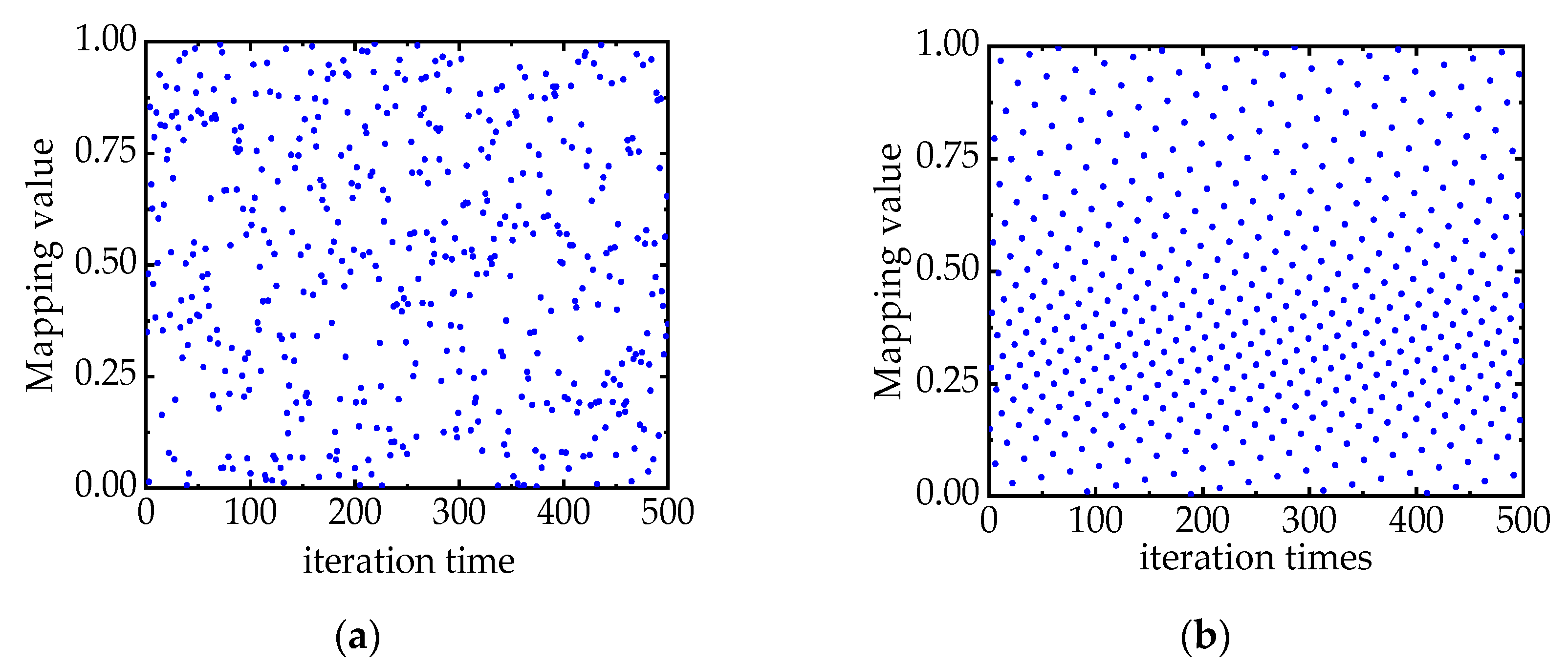
Circle chaotic mapping refers to a process in which the randomly generated population matrix is mathematically mapped into the chaotic domain via the circle mapping formula [28]. Circle chaotic mapping is used to ensure the ergodicity of the individuals of the initial population due to its excellent unpredictable and nonlinear characteristics. The circle mapping formula is introduced in Equation (7).

$$x_{t+1}=x_t+a-\mathrm{mod}(\frac{b}{2\pi }\sin (2\pi \times x_t),1)$$

(7)

where a = 0.2 and b = 0.5.

The individual distribution of the initial population after circle chaotic mapping has ergodicity, as is evident in the comparison between Figure 1a,b. Figure 1b show that the individuals are evenly distributed throughout the search space after 500 iterations, which reduces the risk of AOA falling into the local optimum in a later iteration.

3.2. MOA Optimized by Means of A Compound Cycloid

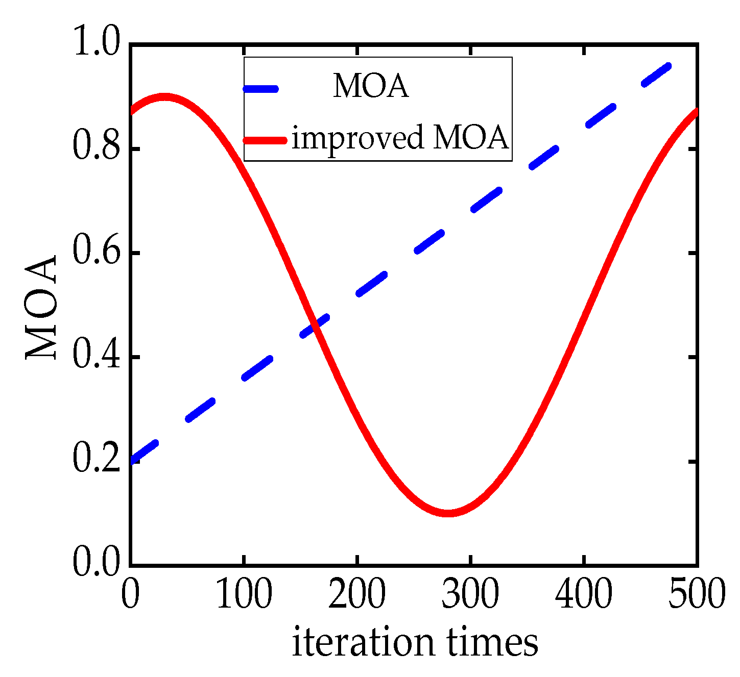
The MOA increases linearly in Equation (2) of the basic AOA, and the minimum value of the MOA is 0.2, and its maximum value is 1 in the iterative process. This leads to a large number of individuals being allocated into the exploitation phase in the early iterations and a large number of individuals being allocated into the exploration phase in the later iterations. In other words, this allocation method leads to an insufficient global search ability and a faster convergence speed. The global search carried out in the later iterations leads to a slow convergence speed, and it is easy for this approach to fall into the local optimum.

A composite cycloid [29] is often used in curve planning because of its flexible form. Here, the curve of a composite cycloid in the vertical direction is utilized to optimize the MOA to solve the above problems. The optimized MOA is expressed as shown in Equation (8).

$$\mathrm{MOA}(t)=1.2-0.8\times \left(\frac{1}{2}-\frac{1}{2}\cos (\frac{2\pi \times (t-a)}{T_{\max }})\right)$$

(8)

where t is the current iteration number, T_max is the final iteration number, and a is the adaptation coefficient.

As shown in Figure 2, the MOA curve optimized using the composite cycloid introduces most of the individuals into the exploration phase in the early iteration so as to improve the global search ability of the algorithm in the early optimization stage. In the middle of the iteration, most of the individuals are introduced into the exploitation phase, which improves the local search ability of the algorithm and increases the convergence rate. In the later iterations, the proportion of individuals entering the exploration phase increases so that some individuals jump out of the local optimum in the late iteration and increase the optimization ability of the algorithm.

The MOA optimized using the compound cycloid demonstrates a strong global search ability in the early iterations. The cosine factor is introduced into the MOA to further improve the algorithm’s performance. The cosine factor c is shown in Equation (9).

$$c=\cos (\frac{\pi \times t}{2\times T_{\max }})$$

(9)

3.3. The Optimal Mutation Strategy, Combining Sparrow Elite Mutation with the Adaptive Water Wave Factor and Cauchy Disturbances

The updating of the individual is affected by the last optimal individual in each iteration in AOA, so in AOA, it is easy to converge to the local optimum in the iteration process. Therefore, we propose the optimal mutation strategy, combining sparrow elite mutation with the adaptive water wave factor and Cauchy disturbances, to solve the above problems.

3.3.1. Sparrow Elite Mutation

The sparrow search algorithm is an efficient swarm intelligence optimization algorithm. Its population consists of a discoverer, a subscriber, and a watchman [30]. The discoverer plays an important role in the sparrow search algorithm (SSA) because of its large optimization space and good optimization ability, which guides the changes in the position of other individuals in SSA.

Elite mutation [31] is a mutation method that presents the abilities of individuals with high search performance to the current optimal individuals. The strong optimization ability (in terms of the discoverer role) is given to the top 20% of the individuals with the current fitness value during each iteration of the AOA. This approach is known as sparrow elite mutation.

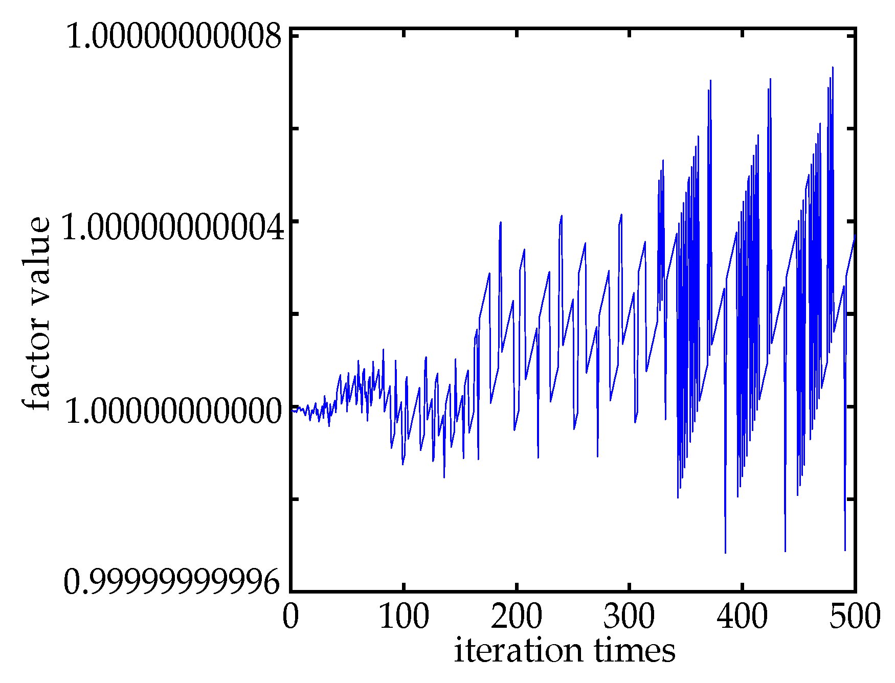
The adaptive water wave factor [16] is added to the updating formula of mutation individuals in order to further increase the optimization ability of the mutation individuals. The water wave factor changes adaptively with the number of iterations. A water wave factor has the characteristics of small fluctuation in the early iteration and large fluctuation in the later iteration. The uncertainty in the iteration process and the violent mutation in the later iterations of the water wave factor enhance the ability of individuals to jump out of the local optimum. The mathematical model of the adaptive water wave factor is:

$$v=1-\sin \left(\frac{\pi \cdot t}{2\cdot T_{\max }}+2\cdot \pi \right)$$

(10)

where v is the adaptive water wave factor, t is the current iteration number, and T_max is the final iteration number.

A water wave factor distribution diagram with 500 iterations is shown in Figure 3.

The individuals in the sparrow elite mutation model will be updated according to Equation (11) after adding the adaptive water wave factor.

$$X_{0.2\cdot best,j}^{t+1}=\{\begin{array}{l}{X}_{0.2\cdot best,j}^t\cdot v\cdot \exp (-\frac{i}{\alpha \cdot T_{\max }}) R<ST\\ X_{0.2\cdot best,j}^t+v\cdot Q\cdot L R\ge ST\end{array}$$

(11)

where X_0.2·best,j is the top 20% of the individuals with the current fitness value, t is the current iteration number, v is the adaptive water wave factor, i is the number of rows in the population matrix where the current individuals are located, and T_max is the final iteration number. Q is a random number obeying a [0,1] normal distribution, L is a 1 × d matrix with all elements 1, R is a random number, ST is a vigilance value, and 0.6 is taken according to experience.

The optimal fitness value after mutation is compared with the fitness value of the current optimal individual. If it is less than the current fitness value, the current optimal individual is mutated to participate in the next update.

3.3.2. Cauchy Disturbance

After the sparrow elite mutation, Cauchy disturbance is conducted in relation to the current optimal individual by introducing the Cauchy operator, which further enhances the optimization performance of AOA. The Cauchy operator is a random variable that satisfies the one-dimensional standard Cauchy–Lorenz distribution [32]. The probability density function is shown in Equation (12).

$$f(x)=\frac{1}{\pi }\times \frac{1}{1+x^2}$$

(12)

As shown in Figure 4, the Cauchy distribution has reasonable probability in all domains, which leads to a stronger mutation effect. However, the probability distributions of some Gaussian normal distributions are concentrated near the origin, not traversing all domains, and the probability distribution of some normal distributions are basically the same in all domains, close to randomly taking values.

The Cauchy distribution formula for the current optimal individual is shown in Equation (13).

$$x_{i,j}^{t+1}=x_{best}^t+cauchy(0,1)\oplus x_{best}^t$$

(13)

where cauchy (0,1) is the Cauchy operator.

The fitness value of an individual after the Cauchy disturbance is thus recalculated. The new fitness value is then compared with the fitness value of the current optimal individual. The individual with the optimal fitness value is selected to participate in the next individual update. The pseudo-code of the improved AOA is as follows (Algorithm 1).

Algorithm 1. The pseudo-code of the improved arithmetic optimization algorithm.
01	Initialization
02	Initialize the population size (n), dimension (m), and the number of iterations (Tmax)
03	Initialize the individuals of population Xi (i = 1, 2, 3, …, n) using circle chaotic mapping, as shown in Equation (7).
04	Evaluate the fitness value and find the current best individual and best fitness value
05	Set the parameters α, μ, ubj, and lbj
06	Main loop{
07	While (t ≤ Tmax)
08	Calculate the MOP by Equation (5)
09	Calculate the MOA by Equations (8) and (9)
10	For each search agent
11	If r1 > MOA
12	Update position by Equation (3)
13	Else
14	Update position by Equation (6)
15	End if
16	Calculate the fitness values of the individuals and rankings according to the fitness values
17	Calculate the water wave factor
18	Update the top 20% of the individuals with the current fitness value according to Equation (11)
19	Update current best individual and best fitness value
20	Disturb the current optimal individual with Equation (13). Compare its fitness value with that before disturbance
21	Update current best individual and best fitness value
22	End for
23	t = t + 1
24	End While}
25	Return best fitness value and current best individual

4. Test of Algorithm

4.1. Effectiveness Test of Algorithm Improvement Strategy

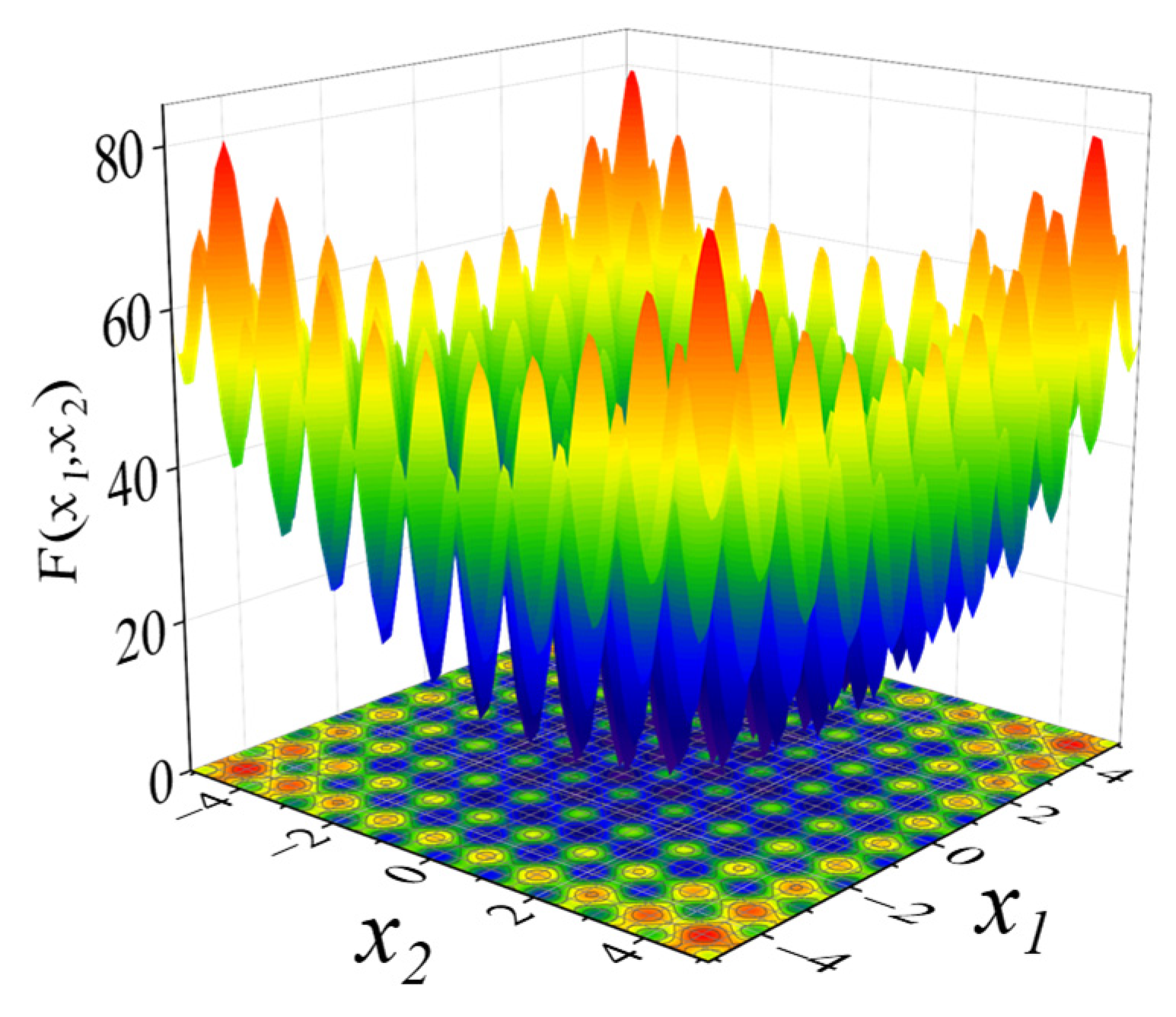
In the arithmetic optimization algorithm combining the compound cycloid and sparrow elite mutation (CSAOA), we apply several strategies to improve the performance of the AOA. The Rastrigin function was selected as the reference test function to verify the effectiveness of these strategies relative to the basic AOA. The Rastrigin function is multi-modal. The difference between the suboptimal value and the global optimal value is large, allowing us to better verify the optimization performance of the CSAOA.

The Rastrigin function is shown in Equation (14), and the range distribution is shown in Figure 5.

$$f(x)=\underset{i=1}{\overset{D}{\Sigma }}(x_i{}^2-10\cos (2\pi \times x_i)+10)\hspace{0.17em}\hspace{0.17em}\hspace{0.17em}\hspace{0.17em}$$

(14)

where x_i ∈ [−5.12,5.12] and D is the total number of x_i.

To ensure the fairness of the optimization environment, 1000 iterations were adopted for each algorithm; the individual dimensions of the population were 30 and 50, separately; and the search area was [−5.12,5.12]. The performance of the algorithm was evaluated based on the mean value and standard deviation.

In the experiment, we adopted the control variable method. CAOA refers to the model only adding the MOA optimized by means of the compound cycloid, as compared with the AOA. SAOA refers to the model only adding the optimal mutation strategy combining the sparrow elite mutation with the adaptive water wave factor and Cauchy disturbance, as compared with the AOA. The mean value of the algorithm reflects the overall convergence speed of the algorithm in the optimization process, and the standard deviation of the algorithm reflects the overall stability of the algorithm in the optimization process. Each strategy was able to find the optimal value, so the optimal value is not reflected in

Table 1. Mean value and standard deviation of different improvement strategies.

Algorithm	Mean Value		Standard Deviation
Dimensional	30	50	30	50
AOA	0.0120	0.0271	0.0312	0.0647
CAOA	9.1050 × 10−5	0.0040	0.0013	0.0041
SAOA	9.5750 × 10−4	0.0017	0.0178	0.0392
CSAOA	1.0912 × 10−7	1.7104 × 10−4	6.8177 × 10−7	1.5102 × 10−10

. Each improvement strategy showed a significant improvement over the performance of the AOA, according to the data in Table 1. The mean value and standard deviation were significantly improved after optimizing the MOA, which proves that CAOA improved the convergence speed and maintained good stability. The convergence rate of SAOA was faster than that of AOA, but the algorithm stability was lower than that of CAOA. However, CSAOA maintained better convergence speed and stability while converging to the optimal value.

4.2. Benchmark Function Test

The performance of CSAOA was checked on 20 benchmark functions. F1–F7 are single-mode benchmark functions that have only one global optimal value, and there is no local optimal value; these were used to test the global search ability and convergence speed of the algorithm. F8–F13 are multi-modal benchmark functions with many local optimal values, and these were used to test the convergence speed of the algorithm and the ability to jump out of the local optimum. F14–F20 are composite fixed low-dimensional test functions, and these were used to test the balanced development ability and stability of the algorithm. The characteristics of some functions are shown in

Table 2. Some of the benchmark functions.

F	Function	Dimensional	Domain	Optimal Value
F1	$f_1(x)={\displaystyle \sum _{i=1}^n{x}_i^2}$	30/100	[−100,100]	0
F2	$f_2(x)={\displaystyle \sum _{i=1}^n\left|x_i\right|}+{\displaystyle \prod _{i=1}^n\left|x_i\right|}$	30/100	[−10,10]	0
F3	$f_3(x)={{\displaystyle \sum _{i=1}^n\left({\displaystyle \sum _{j=1}^i{x}_j}\right)}}^2$	30/100	[−100,100]	0
F4	$f_4(x)=\underset{i}{\max }\left\{\left|x_i\right|,1\le i\le n\right\}$	30/100	[−100,100]	0
F5	$f_5(x)={\displaystyle \sum _{i=1}^{n-1}\left[100{\left(x_{i+1}-x_i^2\right)}^2+{\left(x_i-1\right)}^2\right]}$	30/100	[−30,30]	0
F6	$f_6(x)=x_1^2+{10}^6{\displaystyle \sum _{i=2}^n{x}_i^2}$	30/100	[−10,10]	0
F7	$f_7\left(x\right)={\displaystyle \sum _{i=1}^n}i{x}_i^4+random\left[0,1\right)$	30/100	[−1.28,1.28]	0
F8	$f_8\left(x\right)={\displaystyle \sum _{i=1}^n}\frac{x_i^2}{4000}-{\displaystyle \prod }_{i=1}^n\cos \left(\frac{x_i}{\sqrt{i}}\right)+1$	30/100	[−600,600]	0
F9	$f_9(x)={\displaystyle \sum _{i=1}^n\left[x_i^2-10\cos \left(2\pi x_i\right)+10\right]}$	30/100	[−5.12,5.12]	0
F10	$f_{10}(x)=-20\exp \left(-0.2\sqrt{\frac{1}{n}{\displaystyle \sum _{i=1}^n{x}_i^2}}\right)+\cdots +e$	30/100	[−32,32]	0
F11	$f_{11}(x)=\frac{1}{4000}{\displaystyle \sum _{i=1}^n{x}_i^2}-{\displaystyle \prod _{i=1}^n\cos (\frac{x_i}{\sqrt{i}})}+1$	30/100	[−600,600]	0
F12	$\begin{array}{c}{f}_{12}\left(x\right)=\frac{\pi }{n}\{10\sin \left(\pi y_1\right)+{\displaystyle \sum _{n-1}^{i=1}}{\left(y_i-1\right)}^2[1+10si{n}^2\left(\pi y_{i+1}\right)]+{\left(y_n-1\right)}^2\}\\ +{\displaystyle \sum _n^{i=1}}u\left(x_i,10,100,4\right)\\ y_i=1+\frac{x_i+1}{4}\\ u\left(x_i,a,k,m\right)=\{\begin{array}{cc}k{\left(x_i-a\right)}^m& x_i>a\\ 0& -a<x_i<a\\ k{\left(-x_i-a\right)}^m& x_i<-a\end{array}\end{array}$	30/100	[−50,50]	0
F13	$f_{13}\left(x\right)=0.1\left\{\sin \left(3\pi x_1\right)+\cdots \right\}+{\displaystyle \sum _{i=1}^n}u\left(x_i,5,100,4\right)$	30/100	[−50,50]	0
F14	$f_{14}\left(x\right)={\left(\frac{1}{500}+{\displaystyle \sum _{j=1}^{25}}\frac{1}{j+{\displaystyle \sum _{i=1}^2}{\left(x_i-a_{ij}\right)}^6}\right)}^{-1}$	2	[−65,65]	1
F15	$f_{15}(x)={\displaystyle \sum _{i=1}^{11}\left[a_i-\frac{x_1\left(b_i{}^2+b_1{x}_2\right)}{b_i{}^2+b_1{x}_3+x_4}\right]}$	4	[−5,5]	0.1484
F16	$f_{16}(x)=4x_1^2-2.1x_1^4+\frac{1}{3}{x}_1^6+x_1{x}_2-4x_2^2+4x_2^4$	2	[−5,5]	−1
F17	$f_{17}(x)={\left(x_2-\frac{5.1}{4{\pi }^2}{x}_1^2+\frac{5}{\pi }{x}_1-6\right)}^2+10\left(1-\frac{1}{8\pi }\right)\cos x_1+10$	2	[−5,5]	0.3
F18	$\begin{array}{c}{f}_{18}(x)=\left[1+{\left(x_1+x_2+1\right)}^2\left(19-14x_1+3x_1^2-14x_2+6x_1{x}_2+3x_2^2\right)\right]\\ \times \left[30+{\left(2x_1-3x_2\right)}^2\times \left(18-32x_1+12x_1^2+48x_2-36x_1{x}_2+27x_2^2\right)\right]\end{array}$	2	[−5,5]	3
F19	$f_{19}(x)=-{\displaystyle \sum _{i=1}^4{c}_i^{}}\exp \left(-{\displaystyle \sum _{i=1}^4{a}_{ij}^{}{(x_j-p_{ij})}^2}\right)$	3	[1,3]	−3
F20	$f_{20}\left(x\right)={\displaystyle \sum _{i=1}^5}{\left[\left(X-a_i\right){(X-a_i)}^T+c_i\right]}^{-1}$	4	[0,10]	−1

.

The test dimensions of the algorithms were 30 and 100, except for the composite fixed low-dimensional benchmark functions. AOA, the sparrow search algorithm (SSA), the moth-flame optimization algorithm (MFO), Harris hawks algorithm (HHO), and particle swarm optimization (PSO) were compared with the CSAOA to verify the competitiveness of the CSAOA with other swarm intelligence optimization algorithms. Moreover, two recent optimization techniques for AOA were compared with CSAOA. These were the improved AOA based on an adaptive t-distribution (tAOA) [33] and the improved AOA based on narrowed exploitation (IAOA) [34]. In order to maintain the fairness of the test environment, the software version used was MATLAB 2020a, and the operating system was Microsoft Windows10. The test results of single-mode and multi-mode benchmark functions are exhibited in

Table 3. Comparison of test results of single-mode and multi-mode reference test functions.

F	Algorithm	d = 30			d = 100
		Optimal Value	Standard Deviation	Mean Value	Optimal Value	Standard Deviation	Mean Value
F1	CSAOA	0.0000	0.0000	0.0000	0.0000	0.0000	0.0000
	AOA	1.3697 × 10−2	7.5626 × 10−3	2.2228 × 10−2	2.1635 × 10−2	5.9715 × 10−3	2.8779 × 10−2
	tAOA	6.0359 × 10−243	0.0000	1.3240 × 10−196	2.1929 × 10−244	0.0000	3.4896 × 10−185
	IAOA	2.3852 × 105	1.8367 × 104	2.6226 × 105	2.4203 × 105	1.6107 × 104	2.6472 × 105
	SSA	0.0000	3.8612 × 10−70	1.2210 × 10−70	3.2493 × 10−252	5.8498 × 10−64	2.6161 × 10−64
	MFO	4.1769 × 104	1.1343 × 104	6.1448 × 104	3.8511 × 104	2.0171 × 104	6.4982 × 104
	HHO	1.3821 × 10−108	3.9119 × 10−96	1.3335 × 10−96	5.7961 × 10−103	1.3175 × 10−93	5.8958 × 10−94
	PSO	3.0264 × 103	3.7812 × 103	5.9509 × 103	1.4261 × 103	6.3480 × 103	5.2815 × 103
F2	CSAOA	0.0000	0.0000	0.0000	0.0000	0.0000	0.0000
	AOA	6.7015 × 10−126	4.8715 × 10−65	1.8559 × 10−65	2.9511 × 10−112	1.1059 × 10−87	4.9459 × 10−88
	tAOA	3.7605 × 10−201	2.5231 × 10−103	7.9788 × 10−104	4.9927 × 10−157	2.0300 × 10−118	9.0785 × 10−119
	IAOA	1.1290 × 1035	7.2497 × 1042	2.4022 × 1042	1.2191 × 1037	1.4926 × 1043	6.6814 × 1042
	SSA	0.0000	5.4268 × 10−29	1.7161 × 10−29	0.0000	4.2946 × 10−38	2.0106 × 10−38
	MFO	1.9997 × 102	4.6211 × 101	2.6686 × 102	2.5107 × 102	2.4185 × 101	2.7995 × 102
	HHO	3.7321 × 10−57	4.9387 × 10−53	5.9955 × 10−53	3.9098 × 10−55	1.6429 × 10−51	1.3727 × 10−51
	PSO	1.0347 × 102	4.8000 × 101	1.7509 × 102	1.4143 × 102	5.3238 × 101	2.2226 × 102
F3	CSAOA	0.0000	0.0000	0.0000	0.0000	0.0000	0.0000
	AOA	2.7419 × 10−1	5.3244 × 10−1	6.6035 × 10−1	3.2951 × 10−1	3.9231 × 10−1	7.1837 × 10−1
	tAOA	1.0365 × 10−218	0.0000	9.6478 × 10−176	4.4972 × 10−231	0.0000	1.1412 × 10−173
	IAOA	6.3870 × 105	7.1026 × 104	7.4294 × 105	6.4921 × 105	4.8333 × 104	7.1367 × 105
	SSA	0.0000	0.0000	1.7346 × 10−200	0.0000	6.5412 × 10−122	2.9253 × 10−122
	MFO	1.4995 × 105	9.0594 × 104	2.0952 × 105	1.6427 × 105	4.8054 × 104	2.2954 × 105
	HHO	1.3408 × 10−84	6.6239 × 10−75	2.9892 × 10−75	3.0461 × 10−89	2.1092 × 10−67	9.4328 × 10−68
	PSO	7.8597 × 104	5.0613 × 104	1.3898 × 105	1.2535 × 105	5.9520 × 104	1.6895 × 105
F4	CSAOA	0.0000	0.0000	0.0000	0.0000	0.0000	0.0000
	AOA	7.5159 × 10−2	1.3982 × 10−2	9.1227 × 10−2	8.2203 × 10−2	1.1301 × 10−2	9.3750 × 10−2
	tAOA	2.1545 × 10−115	2.0561 × 10−96	9.2816 × 10−97	3.7202 × 10−104	1.1302 × 10−94	5.0544 × 10−95
	IAOA	9.5448 × 101	7.8251 × 10−1	9.6471 × 101	9.3059 × 101	1.2238	9.4969 × 101
	SSA	0.0000	9.6027 × 10−58	4.2944 × 10−58	0.0000	4.6888 × 10−39	2.0969 × 10−39
	MFO	9.1040 × 101	2.3321	9.4580 × 10	8.9873 × 101	2.1850	9.3124 × 10
	HHO	1.7164 × 10−54	3.8730 × 10−50	1.7338 × 10−50	3.4508 × 10−51	6.1853 × 10−50	5.1528 × 10−50
	PSO	2.0289 × 101	1.4869	2.2811 × 101	1.6643 × 101	4.2802	2.1232 × 101
F5	CSAOA	2.8910 × 10−3	1.2243 × 10−2	1.3436 × 10−2	7.9052 × 10−4	7.6104 × 10−2	5.4217 × 10−2
	AOA	9.8905 × 101	3.1023 × 10−2	9.8941 × 101	9.8819 × 101	6.9540 × 10−2	9.8904 × 101
	tAOA	9.8858 × 101	1.2841 × 10−2	9.8873 × 101	9.8866 × 101	9.0567 × 10−3	9.8875 × 101
	IAOA	1.1471 × 109	4.2754 × 107	1.2011 × 109	1.0705 × 109	1.2350 × 108	1.1855 × 109
	SSA	6.1471 × 10−2	6.4823 × 10−2	1.3251 × 10−1	3.3717 × 10−2	1.9198 × 10−1	1.8190 × 10−1
	MFO	6.5409 × 107	8.6820 × 107	1.8203 × 108	4.0630 × 107	1.1197 × 108	1.7326 × 108
	HHO	3.7312 × 10−3	2.2197 × 10−2	2.6143 × 10−2	1.4050 × 10−3	7.3666 × 10−2	7.9354 × 10−2
	PSO	1.9830 × 105	1.8568 × 107	9.2024 × 106	5.2993 × 105	5.5151 × 105	1.2947 × 106
F6	CSAOA	0.0000	0.0000	0.0000	0.0000	0.0000	0.0000
	AOA	0.0000	0.0000	0.0000	0.0000	0.0000	0.0000
	tAOA	0.0000	0.0000	0.0000	0.0000	0.0000	0.0000
	IAOA	2.7492 × 108	5.9874 × 107	3.3817 × 108	2.9878 × 108	1.0220 × 108	4.0924 × 108
	SSA	0.0000	2.1406 × 10−93	9.5732 × 10−94	1.0696 × 10−286	8.7194 × 10−72	3.8994 × 10−72
	MFO	1.0873 × 104	4.4717 × 107	2.0021 × 107	1.9622 × 104	5.4764 × 107	4.0018 × 107
	HHO	6.6623 × 10−108	7.3828 × 10−98	3.3020 × 10−98	1.1054 × 10−110	1.0168 × 10−94	4.5478 × 10−95
	PSO	1.3601 × 106	3.5205 × 106	5.7181 × 106	4.5861 × 106	4.9289 × 107	4.2768 × 107
F7	CSAOA	2.9267 × 10−6	2.3722 × 10−5	2.8044 × 10−5	9.1698 × 10−6	2.0147 × 10−5	3.5667 × 10−5
	AOA	4.2757 × 10−6	5.9644 × 10−5	5.9879 × 10−5	5.4595 × 10−5	1.3258 × 10−4	2.0102 × 10−4
	tAOA	1.0078 × 10−5	6.4877 × 10−5	6.8564 × 10−5	2.8181 × 10−5	1.1090 × 10−4	9.3297 × 10−5
	IAOA	1.6981 × 103	2.0348 × 102	1.9295 × 103	1.5203 × 103	2.3306 × 102	1.8371 × 103
	SSA	2.6432 × 10−5	4.5348 × 10−4	4.4236 × 10−4	1.7974 × 10−4	3.7072 × 10−4	5.6990 × 10−4
	MFO	1.5975 × 102	1.9347 × 102	2.9386 × 102	1.0539 × 102	1.2845 × 102	2.1167 × 102
	HHO	2.0064 × 10−5	1.2755 × 10−4	1.9150 × 10−4	2.0187 × 10−5	1.2515 × 10−4	1.2073 × 10−4
	PSO	1.0825	5.6768 × 101	4.5013 × 101	9.6292	3.9483 × 101	5.0622 × 101
F8	CSAOA	0.0000	0.0000	0.0000	0.0000	0.0000	0.0000
	AOA	1.3418 × 10−4	2.9923 × 10−4	5.0244 × 10−4	2.9660 × 10−4	1.1015 × 10−4	3.9687 × 10−4
	tAOA	0.0000	0.0000	0.0000	0.0000	0.0000	0.0000
	IAOA	6.3157 × 101	3.2242	6.8351 × 101	6.9486 × 101	2.5146	7.2765 × 101
	SSA	0.0000	0.0000	0.0000	0.0000	0.0000	0.0000
	MFO	1.1117 × 101	3.7540	1.6059 × 101	1.5147 × 101	1.4293	1.6984 × 101
	HHO	0.0000	0.0000	0.0000	0.0000	0.0000	0.0000
	PSO	1.4107	1.7084	2.4831	2.0968	1.4855	3.4349
F9	CSAOA	0.0000	0.0000	0.0000	0.0000	0.0000	0.0000
	AOA	0.0000	0.0000	0.0000	0.0000	0.0000	0.0000
	tAOA	0.0000	0.0000	0.0000	0.0000	0.0000	0.0000
	IAOA	1.6102 × 103	3.1635 × 101	1.6402 × 103	1.5785 × 103	3.3781 × 101	1.6346 × 103
	SSA	0.0000	0.0000	0.0000	0.0000	0.0000	0.0000
	MFO	8.1370 × 102	8.0360 × 101	8.9231 × 102	7.5818 × 102	5.1659 × 101	8.1717 × 102
	HHO	0.0000	0.0000	0.0000	0.0000	0.0000	0.0000
	PSO	8.7786 × 102	9.1631 × 101	9.5337 × 102	9.2307 × 102	6.6515 × 101	9.9908 × 102
F10	CSAOA	8.8818 × 10−16	0.0000	8.8818 × 10−16	8.8818 × 10−16	0.0000	8.8818 × 10−16
	AOA	8.8818 × 10−16	4.7666 × 10−4	2.1317 × 10−4	8.8818 × 10−16	1.0928 × 10−3	1.1372 × 10−3
	tAOA	8.8818 × 10−16	0.0000	8.8818 × 10−16	8.8818 × 10−16	0.0000	8.8818 × 10−16
	IAOA	2.0471 × 101	3.0222 × 10−2	2.0506 × 101	2.0382 × 101	6.4016 × 10−2	2.0477 × 101
	SSA	8.8818 × 10−16	0.0000	8.8818 × 10−16	8.8818 × 10−16	0.0000	8.8818 × 10−16
	MFO	1.9868 × 101	3.3033 × 10−2	1.9924 × 101	1.9755 × 101	7.4727 × 10−2	1.9880 × 101
	HHO	8.8818 × 10−16	0.0000	8.8818 × 10−16	8.8818 × 10−16	0.0000	8.8818 × 10−16
	PSO	1.3243 × 101	1.6071	1.5113 × 101	1.4995 × 101	1.8789	1.7506 × 101
F11	CSAOA	0.0000	0.0000	0.0000	0.0000	0.0000	0.0000
	AOA	1.2203 × 102	2.6186 × 102	4.8193 × 102	2.4244 × 102	2.4150 × 102	4.8551 × 102
	tAOA	0.0000	0.0000	0.0000	0.0000	0.0000	0.0000
	IAOA	2.2522 × 103	1.2950 × 102	2.4163 × 103	2.3306 × 103	1.5393 × 102	2.5064 × 103
	SSA	0.0000	0.0000	0.0000	0.0000	0.0000	0.0000
	MFO	3.7195 × 102	1.2642 × 102	5.1564 × 102	5.0258 × 102	9.5333 × 101	5.7926 × 102
	HHO	0.0000	0.0000	0.0000	0.0000	0.0000	0.0000
	PSO	3.3916 × 101	5.4661	4.1221 × 101	1.9851 × 101	5.5612	2.5891 × 101
F12	CSAOA	0.0000	0.0000	0.0000	0.0000	0.0000	0.0000
	AOA	2.8126	1.6248	4.7728	1.3210	1.4682	3.1535
	tAOA	0.0000	0.0000	0.0000	0.0000	0.0000	0.0000
	IAOA	2.5552 × 105	1.7410 × 104	2.7892 × 105	2.5568 × 105	6.4507 × 103	2.6388 × 105
	SSA	0.0000	0.0000	0.0000	0.0000	0.0000	0.0000
	MFO	5.7450 × 104	1.9759 × 104	7.7476 × 104	3.1256 × 104	1.9452 × 104	6.5136 × 104
	HHO	0.0000	0.0000	0.0000	0.0000	0.0000	0.0000
	PSO	3.4242 × 103	1.4911 × 103	4.5739 × 103	4.2942 × 103	2.1801 × 103	6.7126 × 103
F13	CSAOA	7.7892 × 10−8	5.4511 × 10−5	4.6380 × 10−5	1.0178 × 10−6	2.1624 × 10−5	1.5606 × 10−5
	AOA	9.7578	5.8550 × 10−2	9.8453	9.9285	4.1098 × 10−2	9.9813
	tAOA	9.9859	2.4972 × 10−3	9.9891	9.9841	2.8709 × 10−3	9.9886
	IAOA	4.6601 × 109	4.9023 × 108	5.1856 × 109	4.9443 × 109	4.1623 × 108	5.5553 × 109
	SSA	5.0924 × 10−4	1.0188 × 10−3	1.4685 × 10−3	8.8230 × 10−5	1.1020 × 10−2	5.5947 × 10−3
	MFO	2.1222 × 108	3.4180 × 108	6.0517 × 108	2.7935 × 108	3.9204 × 108	7.0479 × 108
	HHO	4.1771 × 10−6	9.8017 × 10−5	8.9227 × 10−5	5.5344 × 10−6	9.6250 × 10−5	8.4396 × 10−5
	PSO	6.0808 × 101	8.3371 × 104	9.3264 × 104	3.0820 × 102	4.1416 × 104	5.4588 × 104

, and the results of composite fixed low-dimensional benchmark functions are exhibited in

Table 4. Comparison of test results of composite fixed low-dimensional test functions in different iterations.

F	Algorithm	Tmax = 500			Tmax = 1000
		Optimal Value	Standard Deviation	Mean Value	Optimal Value	Standard Deviation	Mean Value
F14	CSAOA	5.9288	1.5366 × 10−13	5.9288	5.9288	3.0150	7.2772
	AOA	7.8740	1.9654	10.9480	5.9288	3.2338	10.3630
	tAOA	9.9800 × 10−1	5.2590	7.6354	2.9821	5.0191	8.4137
	IAOA	9.9801 × 10−1	2.6881 × 10−4	9.9822 × 10−1	9.9800 × 10−1	8.8731 × 10−1	1.3948
	SSA	2.9821	4.3328	10.7330	9.9800 × 10−1	5.6778	8.5956
	MFO	1.9920	1.6460	4.3572	9.9800 × 10−1	2.0442	2.3818
	HHO	9.9800 × 10−1	8.8250 × 10−11	9.9800 × 10−1	9.9800 × 10−1	1.4927 × 10−10	9.9800 × 10−1
	PSO	9.9800 × 10−1	3.2980 × 10−10	9.9800 × 10−1	9.9800 × 10−1	3.0115 × 10−10	9.9800 × 10−1
F15	CSAOA	3.1135 × 10−4	2.2550 × 10−5	3.4556 × 10−4	3.0804 × 10−4	7.7145 × 10−6	3.1364 × 10−4
	AOA	2.0151 × 10−3	7.4864 × 10−3	7.8982 × 10−3	3.3393 × 10−4	9.0278 × 10−3	5.6261 × 10−3
	tAOA	3.3949 × 10−4	9.3537 × 10−3	1.5406 × 10−2	3.8758 × 10−4	1.0277 × 10−3	1.8579 × 10−3
	IAOA	1.5193 × 10−3	3.2671 × 10−3	3.4810 × 10−3	1.5141 × 10−3	8.5690 × 10−4	2.1570 × 10−3
	SSA	3.1621 × 10−4	2.3664 × 10−5	3.3133 × 10−4	3.0826 × 10−4	5.7720 × 10−4	5.7235 × 10−4
	MFO	4.9014 × 10−4	5.1649 × 10−4	1.1770 × 10−3	6.9306 × 10−4	3.8080 × 10−4	1.0286 × 10−3
	HHO	3.2187 × 10−4	4.0765 × 10−5	3.4526 × 10−4	3.1063 × 10−4	2.1931 × 10−5	3.2805 × 10−4
	PSO	1.6554 × 10−3	8.9768 × 10−3	7.3008 × 10−3	1.6554 × 10−3	8.4166 × 10−3	8.6256 × 10−3
F16	CSAOA	−1.0316	2.2288 × 10−11	−1.0316	−1.0316	1.5954 × 10−12	−1.0316
	AOA	−1.0316	1.3946 × 10−7	−1.0316	−1.0316	8.4764 × 10−8	−1.0316
	tAOA	−1.0316	1.6411 × 10−7	−1.0316	−1.0316	1.3202 × 10−7	−1.0316
	IAOA	−1.0290	3.3750 × 10−3	−1.0251	−1.0252	6.4286 × 10−3	−1.0185
	SSA	−1.0316	1.4550 × 10−7	−1.0316	−1.0316	5.9986 × 10−9	−1.0316
	MFO	−1.0316	0.0000	−1.0316	−1.0316	0.0000	−1.0316
	HHO	−1.0316	1.6503 × 10−10	−1.0316	−1.0316	8.2136 × 10−13	−1.0316
	PSO	−1.0316	1.7876 × 10−5	−1.0316	−1.0316	1.2757 × 10−5	−1.0316
F17	CSAOA	3.9789 × 10−1	1.7207 × 10−6	3.9789 × 10−1	3.9789 × 10−1	2.6523 × 10−7	3.9789 × 10−1
	AOA	3.9920 × 10−1	6.9016 × 10−3	4.0607 × 10−1	4.0060 × 10−1	1.0145 × 10−2	4.0984 × 10−1
	tAOA	3.9826 × 10−1	8.4643 × 10−3	4.0736 × 10−1	3.9800 × 10−1	9.1688 × 10−3	4.0481 × 10−1
	IAOA	3.9798 × 10−1	3.8876 × 10−3	4.0362 × 10−1	3.9790 × 10−1	3.5639 × 10−3	4.0178 × 10−1
	SSA	3.9789 × 10−1	7.0847 × 10−7	3.9789 × 10−1	3.9789 × 10−1	3.9668 × 10−8	3.9789 × 10−1
	MFO	3.9789 × 10−1	0.0000	3.9789 × 10−1	3.9789 × 10−1	0.0000	3.9789 × 10−1
	HHO	3.9789 × 10−1	4.3690 × 10−8	3.9789 × 10−1	3.9789 × 10−1	3.9874 × 10−9	3.9789 × 10−1
	PSO	3.9789 × 10−1	1.0920 × 10−6	3.9789 × 10−1	3.9789 × 10−1	4.8865 × 10−1	5.5241 × 10−1
F18	CSAOA	3.0000	6.9354 × 10−11	3.0000	3.0000	4.5769 × 10−11	3.0000
	AOA	3.0000	1.5252 × 10−8	3.0000	3.0000	1.1297 × 101	8.3583
	tAOA	3.0000	1.2072 × 101	8.4046	3.0000	7.5751	5.3955
	IAOA	3.0181	1.3154	4.4153	3.0125	6.8648 × 10−1	3.7742
	SSA	3.0000	1.1655 × 10−6	3.0000	3.0000	1.9297 × 10−7	3.0000
	MFO	3.0000	1.1322 × 10−15	3.0000	3.0000	2.0134 × 10−15	3.0000
	HHO	3.0000	1.0688 × 10−7	3.0000	3.0000	1.5775 × 10−8	3.0000
	PSO	3.0000	1.2094 × 10−4	3.0001	3.0000	2.8097 × 10−5	3.0000
F19	CSAOA	−3.8628	3.4487 × 10−6	−3.8628	−3.8628	2.0503 × 10−6	−3.8628
	AOA	−3.8541	2.0932 × 10−3	−3.8521	−3.8573	3.4847 × 10−3	−3.8524
	tAOA	−3.8589	6.1122 × 10−3	−3.8511	−3.8603	3.1827 × 10−3	−3.8534
	IAOA	−3.8270	1.1869 × 10−1	−3.7383	−3.8493	1.0174 × 10−1	−3.7700
	SSA	−3.8628	2.3691 × 10−5	−3.8628	−3.8628	1.0027 × 10−6	−3.8628
	MFO	−3.8628	0.0000	−3.8628	−3.8628	9.3622 × 10−16	−3.8628
	HHO	−3.8626	4.6271 × 10−4	−3.8618	−3.8628	2.2493 × 10−3	−3.8614
	PSO	−3.8628	3.5228 × 10−3	−3.8612	−3.8628	4.0691 × 10−3	−3.8596
F20	CSAOA	−1.0153 × 101	9.9270 × 10−5	−1.0153 × 101	−1.0153 × 101	1.4965 × 10−5	−1.0153 × 101
	AOA	−5.3422	1.1597	−3.6184	−5.0130	7.2225 × 10−1	−3.5994
	tAOA	−7.9372	1.6177	−5.1167	−9.0817	1.8651	−5.3548
	IAOA	−2.0531	3.1992 × 10−01	−1.5500	−6.8960	1.8733	−2.2640
	SSA	−1.0153 × 101	4.4744 × 10−4	−1.0153 × 101	−1.0153 × 101	6.5870 × 10−5	−1.0153 × 101
	MFO	−1.0153 × 101	2.2595	−9.1427	−1.0153 × 101	3.0171	−7.3715
	HHO	−5.0548	1.1872 × 10−3	−5.0534	−5.0551	1.4752 × 10−3	−5.0541
	PSO	−1.0149 × 101	2.7849	−7.0881	−1.0152 × 101	1.6090	−9.6342

.

The optimal values, mean values, and standard deviations of each algorithm are shown in Table 3 and Table 4, which were used to verify the overall performance of the algorithm. CSAOA showed excellent convergence speed and stability compared with the other algorithms in the single-modal benchmark function, with d = 30. CSAOA found the optimal value with the highest convergence rate and the best stability in F1–F4. Since the parameters of the F5 function were complex, none of the algorithms found the optimal value, but CSAOA approached the optimal value with the highest convergence accuracy, and its convergence speed and stability were among the best. With the increase in the dimensions (d = 100), the convergence speed and stability of each algorithm decreased, but CSAOA still demonstrated better performance than the other algorithms.

In the multi-modal benchmark function with d = 30, the CSAOA found the optimal value with the fastest convergence speed and the best stability in F8–F12. Due to the global uniform distribution of circle chaotic mapping, it converged to the optimal value when the mean and standard deviation were 0 in F8, F9, F11, and F12. SSA and tAOA showed good performance on some simple multi-modal benchmark functions, but CSAOA still showed better performance on complex multi-modal functions, which is similar to its performance in regard to single-mode benchmark functions. The excellent performance of CSAOA in multi-modal benchmark functions fully reflects the role of the MOA optimized by means of compound cycloid and the optimal mutation strategy combining the sparrow elite mutation with the adaptive water wave factor and Cauchy disturbance, with CSAOA demonstrating a stronger ability to jump out of local optimum.

The dimension of the composite fixed low-dimensional function is fixed, and the dimension cannot be changed in the test process. Therefore, higher iterations are selected to test the performance of the algorithm in high-intensity operations. The results are shown in Table 4. For composite fixed low-dimensional benchmark functions, CSAOA showed the highest convergence accuracy compared with the other algorithms except in the case of F14, but the stability of CSAOA was better in the case of F14. When the various algorithms had the same optimization accuracy in other composite fixed low-dimensional benchmark functions, CSAOA maintained a faster convergence speed. However, it was less stable than MFO. CSAOA still has strong competitiveness when the number of iterations is increased.

The convergence curves of each algorithm in some functions are shown in Figure 6 to enable a more intuitive comparison of the competitiveness of CSAOA with various existing mature algorithms. Each algorithm has 500 iterations in Figure 6. CSAOA approached the optimal value at a faster convergence rate under the same conditions, and the fluctuation was small. Furthermore, CSAOA converged to the optimal value with the highest accuracy and stability, except for the case shown in Figure 6e. Although CSAOA fell into the local optimum in Figure 6e, the optimization accuracy also had a good effect, and the stability was higher.

4.3. Time Complexity of the Algorithm

The time complexity of the CSAOA was analyzed to test the solution speed. The total number of individuals is denoted by N, the dimension of each individual is d, and the maximum number of iterations is assumed to be M in the AOA. The time occupied in the initial stage is T₀,

$$T_0=O(n_0+N(f(d)+d\times n_1))$$

(15)

where n₀ is the time required to initialize the algorithm parameters and n₁ is the time required to generate a random number in the algorithm initialization phase. f(d) is the time required to calculate the individual fitness of the initial population.

The time required for individual updating is T₁ after entering the iteration,

$$T_1=O(N(n_2+n_3+n_4)\times d)$$

(16)

where n₂ is the random number generation time required for Equations (2), (3), and (6) in the update process, n₃ is the time required for the updating of the MOA, and n₄ is the time required for individual updating, according to Equations (3) and (6).

The time needed to calculate the fitness value of the new individual is T₂ after updating the individual.

$$T_2=O(N\times f(d))$$

(17)

The time complexity required by the AOA is obtained through the above analysis as Equation (18).

$$T_w=T_0+M\times (T_1+T_2)=O(d+f(d))$$

(18)

The time complexity of CSAOA in initialization is expressed as T_0′,

$$T_0\prime =O(t_0+N(f(d)+d\times t_1))$$

(19)

where t₀ is the time required to initialize the algorithm parameters and t₁ is the time required to generate a random number when the algorithm is initialized. It can be seen from Equation (19) that the introduction of the circle chaotic approach did not increase the algorithm’s time complexity.

The time required for individual updating is T_1′ after entering the iteration,

$$T_1\prime =O(N((t_2+t_3+t_4)\times d+f(d)))$$

(20)

where t₂ is the random number generation time required for Equations (2), (3), and (6) in the updating process, t₃ is the time required for the MOA optimized by compound cycloid updating, and t₄ is the time required for individual updating, according to Equations (3) and (6).

The time complexity of the sparrow elite mutation with the adaptive water wave factor is calculated as:

$$T_2\prime =O(t_5+t_6+t_7+f(d))\times d))$$

(21)

where t₅ is the generation time of the adaptive water wave factor, t₆ is the generation time of the random number in sparrow elite mutation, and t₇ is the time required for the individual updating process according to Equation (11).

The time complexity of the Cauchy disturbance performed on the optimal individual in the population is:

$$T_3\prime =O(0.1\times N(t_8+f(d))\times d))$$

(22)

where t₈ is the time required for the individual to perform the Cauchy disturbance.

In summary, the time complexity of CSAOA is expressed as T_w’.

$$T_w\prime =T_0\prime +M\times (T_1\prime +T_2\prime +T_3\prime )\hspace{0.17em}=O(d+f(d))$$

(23)

CSAOA had the same time complexity as AOA, comparing the time complexity before and after improvement, which proves that CSAOA (representing the algorithm after multi-strategy improvement) does not increase the time complexity of the AOA.

4.4. Wilcoxon Rank-Sum Test

Three single-mode benchmark functions and three multi-mode benchmark functions were selected to perform the Wilcoxon rank-sum test for all algorithms. The rank-sum test was performed under the conditions of p = 5% and d = 30 to compare the optimization effect between CSAOA and other algorithms.

Firstly, we established assumptions H0 and H1, with H0 indicating that the optimization effects of the two algorithms were not significantly different and H1 indicating that the optimization effects of the two algorithms were significantly different. H0 was rejected, and H1 was accepted when p < 5%; otherwise, H0 was accepted, and H1 was rejected.

CSAOA was tested through Wilcoxon rank-sum tests with five algorithms, respectively. The p-values are shown in

Table 5. The p-values of the Wilcoxon rank-sum tests.

F	AOA	tAOA	IAOA	SSA	MFO	HHO	PSO
F1	1.2118 × 10−12	1.2118 × 10−12	1.2118 × 10−12	1.7016 × 10−8	1.2118 × 10−12	1.2118 × 10−12	1.2118 × 10−12
F2	1.2118 × 10−12	1.2118 × 10−12	1.2118 × 10−12	1.6572 × 10−11	1.2118 × 10−12	1.2118 × 10−12	1.2118 × 10−12
F3	1.2118 × 10−12	1.2118 × 10−12	1.2118 × 10−12	3.4526 × 10−7	1.2118 × 10−12	1.2118 × 10−12	1.2118 × 10−12
F4	1.2118 × 10−12	1.2118 × 10−12	1.2118 × 10−12	5.7720 × 10−11	1.2118 × 10−12	1.2118 × 10−12	1.2118 × 10−12
F8	1.2118 × 10−12	NAN	1.2118 × 10−12	NAN	1.2118 × 10−12	NAN	1.2118 × 10−12
F9	NAN	NAN	1.2118 × 10−12	NAN	1.2118 × 10−12	NAN	1.2118 × 10−12
F10	3.1335 × 10−4	NAN	1.2118 × 10−12	NAN	1.2118 × 10−12	NAN	8.9713 × 10−13
F11	1.2118 × 10−12	NAN	1.2118 × 10−12	NAN	1.2118 × 10−12	NAN	1.2118 × 10−12
F20	1.2118 × 10−12	1.7769 × 10−10	3.0199 × 10−11	8.8411 × 10−7	1.5510 × 10−1	4.0772 × 10−11	2.6099 × 10−10

.

NAN represents the same optimization ability as the two algorithms in Table 5.

The Wilcoxon rank-sum test results indicated that most of the p-values of the nine test functions were less than 5%, indicating that the test results enabled us to reject the H0 hypothesis and accept the H1 hypothesis. This also proves that the results of CSAOA and the other algorithms had significant differences. CSAOA proved to be more effective than the other algorithms, combining the previous test results. Only the p-values of SSA and tAOA were slightly higher than other algorithms, but they were all less than 5%. This result proves that the significant differences among SSA, tAOA, and CSAOA were slightly smaller than other algorithms, which is consistent with the previous tests.

4.5. CEC2019 Test Set

CEC2019 is a set of test functions proposed by the Congress on Evolutionary Computation in 2019 (CEC 2019) to test the performance of algorithms [35]. CSAOA, AOA, tAOA, IAOA, SSA, MFO, HHO, and PSO were brought separately into the CEC2019 test set under the same conditions to verify the robustness of CSAOA. The CEC2019 test set consists of functions with complex spatial characteristics and different dimensions, and the optimal value of each function is 1. Each function was iterated 500 times and independently repeated 30 times. The test results are shown in

Table 6. CEC2019 test results.

Function	Dimensional	Algorithm	Optimal Value	Standard Deviation	Mean Value
CEC01	9	CSAOA	1.0000	9.9362 × 10−11	1.0000
		AOA	1.0000	2.0992 × 101	1.9396
		tAOA	1.0000	5.9761 × 103	6.3787 × 102
		IAOA	7.6618 × 103	1.5845 × 104	1.5918 × 104
		SSA	1.0000	9.5074 × 101	5.2818
		MFO	2.7674 × 101	5.3492 × 103	1.1279 × 103
		HHO	1.0000	1.7750 × 104	1.2836 × 103
		PSO	5.1698 × 102	7.9872 × 103	2.0578 × 103
CEC02	16	CSAOA	4.3008	1.9870 × 10−1	4.4720
		AOA	4.8822	3.0697	5.3359
		tAOA	4.6721	6.1232	5.2510
		IAOA	5.4774 × 101	1.4310 × 101	6.2534 × 101
		SSA	5.0000	6.1930 × 10−1	5.0301
		MFO	6.4186 × 101	2.3793 × 101	7.1883 × 101
		HHO	5.0000	1.3384 × 101	6.1740
		PSO	2.4646 × 101	1.0274 × 101	3.2307 × 101
CEC03	18	CSAOA	1.4791	3.0558	4.2609
		AOA	4.4274	8.0300 × 10−1	4.6550
		tAOA	5.8347	1.2666	6.5828
		IAOA	1.2712 × 101	1.0040 × 10−1	1.2730 × 101
		SSA	5.6212	9.5340 × 10−1	6.6439
		MFO	1.0712 × 101	7.3540 × 10−1	1.1880 × 101
		HHO	8.2746	6.7500 × 10−1	8.6720
		PSO	9.4749	4.9620 × 10−1	9.6062
CEC04	10	CSAOA	3.7850 × 101	2.4151 × 101	6.1721 × 101
		AOA	6.4291 × 101	5.8293	6.6431 × 101
		tAOA	3.2929 × 101	6.4355	3.5815 × 101
		IAOA	5.0192 × 101	2.1434 × 101	6.1235 × 101
		SSA	7.4627 × 101	6.5244	7.6946 × 101
		MFO	6.2439 × 101	1.2302 × 101	6.5784 × 101
		HHO	5.7328 × 101	1.5165 × 101	7.3943 × 101
		PSO	6.4824 × 101	7.0026	6.9592 × 101
CEC05	10	CSAOA	1.3758 × 101	4.2440 × 101	4.0781 × 101
		AOA	5.7798 × 101	2.2018	5.8757 × 101
		tAOA	2.8283 × 101	2.5955	2.8973 × 101
		IAOA	1.2654 × 101	1.6715 × 101	2.0529 × 101
		SSA	1.6138 × 101	3.7191 × 101	3.7237 × 101
		MFO	1.0359 × 101	2.6354 × 101	1.6591 × 101
		HHO	1.6947	1.8314 × 101	1.9929 × 101
		PSO	2.0462 × 101	1.4811 × 101	2.3161 × 101

.

The test results showed that CSAOA displayed the highest relative optimization accuracy in the solution process and maintained a relatively higher convergence speed and stability, except for the case of CEC05 and CEC04. CSAOA has many operation parameters, and AOA has difficulty solving CEC05, which results in a slightly lower convergence accuracy than MFO and HHO. However, compared with AOA, performance was greatly improved.

5. Engineering Application of Algorithm

5.1. The Problem of AC Motor PID Control

Swarm intelligence optimization algorithms are usually used to optimize control systems in the engineering field. Aiming at the stability problem of AC motor PID control, CSAOA was applied to the parameter tuning of the PID controller to ensure the stable operation of the system. The mathematical model of the AC motor is displayed in Figure 7 [36].

Where the driver proportional coefficient K_P1 is 10, the time constant T_p1 is 0.2, the inertia J = 2.5 × 10⁶ kg·m², the current loop proportional coefficient K_i = 5, the proportional coefficient K_t = 0.3, K_u = 1, and the feedback coefficient K_p = 0.001.

The control expression of PID, applied in practical engineering, is shown in Equation (24),

$$u(k)=K_{p}e(k)+K_i{\displaystyle {\sum }_{n=0}^{K}e(k)}+K_d\left[e(k)-e(k-1)\right]$$

(24)

where K_p is the proportional coefficient, K_i is the integral coefficient, and K_d is a differential coefficient.

AOA, tAOA, IAOA, SSA, MFO, HHO, PSO, and CSAOA were utilized separately to tune the parameters of this PID control system, and then the results were compared. The initial conditions of each algorithm were consistent, the number of individuals was 30, and the maximum number of iterations was 100. Each algorithm was run 30 times independently, and the mean values of the results were taken. The parameter tuning results of this PID control system are shown in

Table 7. Comparison of parameter setting results of different algorithms applied to PID control of an AC motor.

Algorithm	Kp	Ki	Kd	Fitness Value
CSAOA	0.0000	0.0238	0.5000	120.3124
AOA	0.4074	0.3279	0.2194	127.4984
tAOA	0.0604	0.0000	0.5000	123.3777
IAOA	0.4074	0.0788	0.3279	126.2875
SSA	0.4074	0.0439	0.1230	127.4984
MFO	0.4074	0.3279	0.2194	127.4984
HHO	0.4074	0.3279	0.2194	127.4984
PSO	0.4074	0.3279	0.2194	127.4984

.

As shown in Figure 8, CSAOA displayed the best tuning effect on the parameters of the PID controller. The system reached the expected value with the minimum rise time after CSAOA optimization, and the overshoot and oscillation values were the smallest.

5.2. Pressure Vessel Design Problem

Pressure vessel design is a common problem in engineering design [37]. The goal of pressure vessel design is to minimize the production costs of the pressure vessel under the premise of meeting the pressure conditions. The design of a pressure vessel is shown in Figure 9. The pressure vessel design problem has four variables to be optimized, namely, L, R, T_s, and T_h. L is the length of the tube, R is the inner wall diameter of the cylindrical part, T_s is the wall thickness of the cylindrical part of the pressure vessel, and T_h is the wall thickness of the pressure vessel head. The objective function of the problem is exhibited in Equations (25) and (26). The constraint conditions are shown in Equations (27) to (30),

$$x=\left[x_1,x_2,x_3,x_4\right]=\left[T_s,T_h,R,L\right]$$

(25)

$$f(x)=0.6224x_1{x}_3{x}_4+1.7781x_2{x}_3^2+3.1661x_1^2{x}_4+19.84x_1^2{x}_3$$

(26)

$$g_1(x)=-x_1+0.0193x_3\le 0$$

(27)

$$g_2(x)=-x_2+0.00954x_3\le 0$$

(28)

$$g_3(x)=-\pi x_3^2-4\pi x_3^3/3+1296000\le 0$$

(29)

$$g_4(x)=x_4-240\le 0$$

(30)

where the search range for x₁, x₂, x₃, x₄ is shown in (31).

$$0\le x_1\le 99,\hspace{0.17em}0\le x_2\le 99,\hspace{0.17em}10\le x_3\le 100,\hspace{0.17em}10\le x_4\le 100$$

(31)

Table 8. Optimization results of the pressure vessel problem.

Algorithm	Ts	Th	R	L	Fitness Value
CSAOA	1.3250	0.7248	67.6089	10.0440	8861.4469
tCAOA	1.6194	0.6908	70.5038	10.0000	10,567.4419
IAOA	1.3543	0.6834	69.3791	10.0000	9016.5015
AOA	1.9331	0.7133	68.6411	67.5328	17,440.9848
SSA	1.3023	0.6437	67.4747	24.0520	8925.9204
MFO	1.3006	0.6473	67.3861	100.0000	13,478.2491
HHO	1.3031	0.6469	67.3860	65.6424	11,433.7792
PSO	1.9304	0.9545	100.0000	10.0000	25,684.5813

show the optimization results of the pressure vessel problem. CSAOA found the most suitable solution compared with the other algorithms, followed by SSA and IAOA. The results in Table 8 show that CSAOA displayed better performance in practical engineering applications.

6. Conclusions

An improved arithmetic optimization algorithm combining a compound cycloid and sparrow elite mutation (CSAOA) was proposed in this paper. The novel improved AOA displays a high convergence accuracy, fast speed, and strong stability.

In this improved AOA, the initialization method based on circle chaotic mapping makes the distribution of the initial population more uniform. The global search ability is enhanced, and the convergence speed is accelerated through the use of an MOA optimized by means of a compound cycloid. The optimal mutation strategy is proposed to improve the problems of falling easily into the local optimum and the low convergence accuracy.

The convergence accuracy, convergence speed, and stability of the CSAOA were proven to be excellent compared with other algorithms, based on 20 benchmark functions, solved separately using CSAOA, AOA, tAOA, IAOA, SSA, MFO, HHO, and PSO. The time complexity of the algorithm, the significant difference in the running results of each algorithm, and the optimization effect for functions of a high level of difficulty were further verified through the use of a time complexity test, rank-sum test, and the CEC2019 test set, respectively. Finally, the effectiveness of the practical application of the CSAOA was verified through engineering examples.

Improving the updating formula of the individual population will be the focus of future work. The algorithm will be made to jump out of the limit of the updating formula by improving the updating formula of the algorithm. This will further improve the searching ability of the algorithm in each iteration’s updating process.

References

- Chaudhary, K.; Chaudhary, H. Optimal dynamic design of planar mechanisms using teaching learning based optimization algorithm. Proc. Inst. Mech. Eng. Part C J. Mech. Eng. Sci. 2016, 230, 3442–3456. [Google Scholar] [CrossRef]
- Wang, B.; Xiang, T.; Li, N. A Symmetric Sine Cosine Algorithm with Adaptive Probability Selection. IEEE Access 2020, 8, 25272–25285. [Google Scholar] [CrossRef]
- Hekimoğlu, B. Sine-cosine algorithm-based optimization for automatic voltage regulator system. Trans. Inst. Meas. Control 2018, 41, 1761–1771. [Google Scholar] [CrossRef]
- Ye, A.; Zhou, X.; Miao, F. Innovative Hyperspectral Image Classification Approach Using Optimized CNN and ELM. Electronics 2022, 11, 775. [Google Scholar] [CrossRef]
- Ahmadianfar, I.; Heidari, A.A.; Gandomi, A.H.; Chu, X.; Chen, H. RUN beyond the metaphor: An efficient optimization algorithm based on Runge Kutta method. Expert Syst. Appl. 2021, 181, 115079. [Google Scholar] [CrossRef]
- Wongkhuenkaew, R.; Auephanwiriyakul, S.; Chaiworawitkul, M.; Theera-Umpon, N. Three-Dimensional Tooth Model Reconstruction Using Statistical Randomization-Based Particle Swarm Optimization. Appl. Sci. 2021, 11, 2363. [Google Scholar] [CrossRef]
- Kotyrba, M.; Volna, E.; Habiballa, H.; Czyz, J. The Influence of Genetic Algorithms on Learning Possibilities of Artificial Neural Networks. Computers 2022, 11, 70. [Google Scholar] [CrossRef]
- Bu, S.J.; Kang, H.B.; Cho, S.B. Ensemble of Deep Convolutional Learning Classifier System Based on Genetic Algorithm for Database Intrusion Detection. Electronics 2022, 11, 745. [Google Scholar] [CrossRef]
- Fan, Q.; Chen, Z.; Xia, Z. A novel quasi-reflected Harris hawks optimization algorithm for global optimization problems. Soft Comput. 2020, 24, 14825–14843. [Google Scholar] [CrossRef]
- Hussain, K.; Zhu, W.; Salleh, M. Long-Term Memory Harris’ Hawk Optimization for High Dimensional and Optimal Power Flow Problems. IEEE Access 2019, 7, 147596–147616. [Google Scholar] [CrossRef]
- Yi, H.; Wang, J.; Hu, Y. Mechanism isomorphism identification based on artificial fish swarm algorithm. Proc. Inst. Mech. Eng. Part C J. Mech. Eng. Sci. 2021, 235, 5421–5433. [Google Scholar] [CrossRef]
- Ouyang, C.; Zhu, D.; Qiu, Y. Lens Learning Sparrow Search Algorithm. Math. Probl. Eng. 2021, 2, 9935090. [Google Scholar] [CrossRef]
- Song, C.; Yao, L.; Hua, C. Comprehensive water quality evaluation based on kernel extreme learning machine optimized with the sparrow search algorithm in Luoyang River Basin, China. Environ. Earth Sci. 2021, 80, 16. [Google Scholar] [CrossRef]
- Xu, X.; Peng, L.; Ji, Z. Research on Substation Project Cost Prediction Based on Sparrow Search Algorithm Optimized BP Neural Network. Sustainability 2021, 13, 13746. [Google Scholar] [CrossRef]
- Meidani, K.; Hemmasian, A.; Mirjalili, S.; Barati Farimani, A. Adaptive grey wolf optimizer. Neural Comput. Appl. 2022, 34, 7711–7731. [Google Scholar] [CrossRef]
- He, Q.; Luo, S. Hybrid improved chimpanzee optimization algorithm and its mechanical application. Control Decis. 2022, 1, 11. [Google Scholar]
- Jia, H.; Sun, K.; Zhang, W.; Leng, X. An enhanced chimp optimization algorithm for continuous optimization domains. Complex Intell. Syst. 2022, 8, 65–82. [Google Scholar] [CrossRef]
- Wang, W.C.; Xu, L.; Chau, K.W. Yin-Yang firefly algorithm based on dimensionally Cauchy mutation. Expert Syst. Appl. 2020, 150, 113216. [Google Scholar] [CrossRef]
- Zhang, Y.; Chen, F. A Modified Whale Optimization Algorithm. Comput. Eng. 2018, 44, 208–213. [Google Scholar]
- Saremi, S.; Mirjalili, S.Z.; Mirjalili, S.M. Evolutionary population dynamics and grey wolf optimizer. Neural Comput. Appl. 2015, 26, 1257–1263. [Google Scholar] [CrossRef]
- Mirjalili, S.; Saremi, S.; Mirjalili, S.M. Multi-objective grey wolf optimizer: A novel algorithm for multi-criterion optimization. Expert Syst. Appl. 2016, 47, 106–119. [Google Scholar] [CrossRef]
- Abualigah, L.; Diabat, A.; Mirjalili, S. The arithmetic optimization algorithm. Comput. Methods Appl. Mech. Eng. 2021, 376, 113609. [Google Scholar] [CrossRef]
- Lan, Z.; He, Q. Multi-trategy Fusion Algorithm and Its Engineering Optimization. Appl. Res. Comput. 2022, 39, 758–763. [Google Scholar]
- Yang, W.; He, Q. Optimization algorithm of multi-head reverse series algorithm with activation mechanism. Appl. Res. Comput. 2022, 39, 151–156. [Google Scholar]
- Abualigah, L.; Diabat, A.; Sumari, P. A Novel Evolutionary Arithmetic Optimization Algorithm for Multilevel Thresholding Segmentation of COVID-19 CT Images. Processes 2021, 9, 1155. [Google Scholar] [CrossRef]
- Khatir, S.; Tiachacht, S.; Thanh, C.L.; Ghandourah, E.; Wahab, M.A. An improved artificial neural network using arithmetic optimization algorithm for damage assessment in FGM composite plates. Compos. Struct. 2021, 273, 114287. [Google Scholar] [CrossRef]
- Zheng, R.; Jia, H.; Abualigah, L.; Liu, Q.; Wang, S. An improved arithmetic optimization algorithm with forced switching mechanism for global optimization problems. Math. Biosci. Eng. 2022, 19, 473–512. [Google Scholar] [CrossRef]
- Li, S.Y.; Gu, K.R. Smart Fault-Detection Machine for Ball-Bearing System with Chaotic Mapping Strategy. Sensors 2019, 19, 2178. [Google Scholar] [CrossRef] [Green Version]
- Dósa, G.; Newman, N.; Tuza, Z.; Voloshin, V. Coloring Properties of Mixed Cycloids. Symmetry 2021, 13, 1539. [Google Scholar] [CrossRef]
- Li, M.; Liu, Z.; Wang, M.; Pang, G.; Zhang, H. Design of a Parallel Quadruped Robot Based on a Novel Intelligent Control System. Appl. Sci. 2022, 12, 4358. [Google Scholar] [CrossRef]
- Feng, Z.K.; Liu, S.; Niu, W.J.; Liu, Y.; Luo, B.; Miao, S.M.; Wang, S. Optimal Operation of Hydropower System by Improved Grey Wolf Optimizer Based on Elite Mutation and Quasi-Oppositional Learning. IEEE Access 2019, 7, 155513–155529. [Google Scholar] [CrossRef]
- Martín, J.; Parra, M.I.; Pizarro, M.M.; Sanjuán, E.L. Baseline Methods for the Parameter Estimation of the Generalized Pareto Distribution. Entropy 2022, 24, 178. [Google Scholar] [CrossRef] [PubMed]
- Zheng, T.; Liu, S.; Ye, X. Improved arithmetic optimization algorithm of adaptive t distribution and dynamic boundary strategy. Comput. Appl. Res. 2022, 39, 1410–1414. [Google Scholar]
- Abbassi, A.; Ben Mehrez, R.; Bensalem, Y.; Abbassi, R.; Kchaou, M.; Jemli, M.; Abualigah, L.; Altal, M. Improved Arithmetic Optimization Algorithm for Parameters Extraction of Photovoltaic Solar Cell Single-Diode Model. Arab. J. Sci. Eng. 2022, 139, 1–17. [Google Scholar] [CrossRef]
- Bezdan, T.; Stoean, C.; Naamany, A.A.; Bacanin, N.; Rashid, T.A.; Zivkovic, M.; Venkatachalam, K. Hybrid Fruit-Fly Optimization Algorithm with K-Means for Text Document Clustering. Mathematics 2021, 9, 1929. [Google Scholar] [CrossRef]
- Wang, Y. Study on Pressure Balance Control of Piston Pressure Sensor. Master’s Thesis, Hefei University of Technology, Hefei, China, 2018. [Google Scholar]
- Kıran, M.S. An Implementation of Tree-Seed Algorithm (TSA) for Constrained Optimization. Intell. Evol. Syst. 2016, 5, 189–197. [Google Scholar] [CrossRef]
Figure 1.
(a) Individual distribution map using random generation. (b) Individual distribution map using circle chaotic mapping.
Figure 2.
Comparison of optimized MOA curves before and after improvement.
Figure 3.
Adaptive water wave factor distribution with 500 iterations.
Figure 4.
Probability density plots of standard Cauchy distribution and various Gaussian normal distributions.
Figure 5.
Rastrigin function value distribution diagram.
Figure 6.
Convergence curves of different algorithms on different functions. The selected functions were those with obvious differences between the convergence curves of each algorithm. (a) F2 function; (b) F3 function; (c) F7 function; (d) F10 function; (e) F15 function; (f) F20 function.
Figure 7.
AC motor mathematical model.
Figure 8.
Optimization results of different algorithms in engineering examples.
Figure 9.
The model of the pressure vessel problem.