Control Analysis of Stochastic Lagging Discrete Ecosystems

Abstract

In this paper, control analysis of a stochastic lagging discrete ecosystem is investigated. Two-dimensional stochastic hysteresis discrete ecosystem equilibrium points with symmetry are discussed, and the dynamical behavior of equilibrium points with symmetry and their control analysis is discussed. Using the orthogonal polynomial approximation theory, the stochastic lagged discrete ecosystems are approximately transformed as its equivalent deterministic ecosystem. Based on the stability and bifurcation theory of deterministic discrete systems, through mathematical analysis, asymptotic stability and Hopf bifurcation are existent in the ecosystem, constructing control functions, controlling the behavior of the system dynamics. Finally, the effects of different random strengths on the bifurcation control and asymptotic stability control are verified by numerical simulations, which validate the correctness and effectiveness of the main results of this paper.

1. Introduction

The ecosystem provides the natural environment on which human beings depend for survival. In recent years, ecological complexity is a new hot topic in international ecological research [1,2,3], and its basic idea is to understand the dynamic behavior of ecosystems. Ecosystems are typically complex systems, and internal interactions lead to the complexity of ecosystems. In ecology, branching and chaotic phenomena often correspond to the catastrophe of the studied species, so there has been a growing interest in the study of mathematical ecology. In economics, ecosystems, mechanics and aviation, dynamics play an important role [4,5,6,7,8,9].

In 1976, May studied simple mathematical models with very complicated dynamics and had a paper published in Nature [10], which established that many ecosystems were remarkable complexity in dynamics. The Wang et al. analysis of dynamic and bifurcation in an ecosystem is investigated in reference [11]. Reference [12] studied stochastically globally exponential stability for stochastic impulsive differential systems. In reference [13], the control of a hyperchaotic discrete system is investigated. Tie and Lin are studied controllability of two-dimensional discrete-time bilinear systems [14]. Reference [15] studies the stability of two-dimensional discrete systems. Ooba studied asymptotic stability of two-dimensional discrete systems with saturation nonlinearities [16]. Jia et al. investigate the stochastic dynamics of a prey–predator type ecosystem driven by Poisson white noise excitation [17]. Wan studied an iterative learning control of two-dimensional discrete systems in the general model [18]. Wang et al. studied dynamic analysis of the coupled logistic map [19]. Reference [20] studied the logistic mapping bifurcation control. Wang et al. studied chaos control of two dimensional logistic mapping in references [21]. The dynamical behavior of discrete systems and their control are studied in references [22,23,24]. In the ecosystem, because these stochastic factors cannot be ignored, various stochastic ecosystems will be considered. In the real world, the stochastic factors determine the changing trends of ecosystems, and delays exist in ecosystems. Thus, it is very necessary to research the dynamical behavior in lagged discrete ecosystems with random parameters. In recent years, Xu et al. have studied the dynamic behavior and dynamic control problems of systems with random parameters. For instance, bifurcation, chaos and so on [25,26,27,28]. In particular, Ma et al. is investigated stochastic Hopf bifurcation behavior of a stochastic lagged logistic system [29].

Motivated by the above discussion, and inspired by reference [29], we consider control analysis of a stochastic lagged discrete ecosystem with a random parameter, the influence of a random parameter in the stochastic lagged discrete ecosystem on bifurcation control and asymptotic stability control is investigated by orthogonal polynomial approximation.

2. Materials and Methods

The Lagged Discrete Ecosystem with Random Parameter and Its Orthogonal Polynomial Approximation

In reference [29], the authors considered two-dimensional lagged discrete ecosystems, as follows:

$$\{\begin{array}{l}{z}_1(n+1)=z_2(n),\\ z_2(n+1)=\overline{\mu }{z}_2(n)(1-z_1(n)),\end{array}\left(\overline{\mu }\in (0,2.28),z_1,z_2\in (0,1)\right).$$

(1)

Obviously, the system (1) has only one fixed point $S(1-1/\overline{\mu },1-1/\overline{\mu })$. In order to facilitate the system dynamics behavior and control analysis, we use the coordinate transformation, $S$ is transformed to the origin $O(0,0)$, and then we have

$$\{\begin{array}{l}x(n+1)=y(n),\\ y(n+1)=y(n)-(\overline{\mu }-1)x(n)-\overline{\mu }x(n)y(n),\end{array}$$

(2)

Adding a linear control term to Equation (2) yields the controlled system as

$$\{\begin{array}{l}x(n+1)=y(n)+Kx(n),\\ y(n+1)=y(n)-(\overline{\mu }-1)x(n)-\overline{\mu }x(n)y(n)+Ky(n),\end{array}$$

(3)

denotes the linear control term as

$$U(\ast )=K\left[\begin{array}{c}x(n)\\ y(n)\end{array}\right],$$

(4)

and $K\ne 0$, and where $\overline{\mu }$ is a random parameter which can be described as

$$\overline{\mu }=\mu +\delta k,$$

(5)

where $\mu$ is the deterministic system parameter about $\overline{\mu }$, $\delta$ is regarded as strength of random disturbance, and $k$ is a random variable which obeys density function of the Poisson distribution $p_k$ with standard deviation $\lambda$.

Therefore, under condition of the convergence in mean square, it follows from the orthogonal polynomial approximation that the solution of (3) can be expressed as following

$$\{\begin{array}{l}x(n,k)={\displaystyle \sum _{i=0}^M{x}_i(n)Q_i(k)},\\ y(n,k)={\displaystyle \sum _{i=0}^M{y}_i(n)Q_i(k)},\end{array}$$

(6)

where $x_i(n)={\displaystyle \sum _{k=0}^N{p}_{k}x(n,k)}{Q}_i(k),y_i(n)={\displaystyle \sum _{k=0}^N{p}_{k}y(n,k)}{Q}_i(k),$ $Q_i(k)$ is the ith Charlier orthogonal polynomial, $M$ represents order of the polynomial.

Substituting (5) and (6) into (3), we obtain

$$\{\begin{array}{l}{\displaystyle \sum _{i=0}^M{x}_i(n+1)Q_i(k)}={\displaystyle \sum _{i=0}^M{y}_i(n)Q_i(k)}+K{\displaystyle \sum _{i=0}^M{x}_i(n)Q_i(k),}\\ {\displaystyle \sum _{i=0}^M{y}_i(n+1)Q_i(k)}={\displaystyle \sum _{i=0}^M{y}_i(n)Q_i(k)-(\mu +\delta k-1){\displaystyle \sum _{i=0}^M{x}_i(n)Q_i(k)}}\\ -(\mu +\delta k)\left({\displaystyle \sum _{i=0}^M{x}_i(n)P_i(k){\displaystyle \sum _{i=0}^M{y}_i(n)Q_i(k)}}\right)+K{\displaystyle \sum _{i=0}^M{y}_i(n)Q_i(k)}.\end{array}$$

(7)

According to a cycle recurrence formula of Charlier polynomial

$$k{Q}_i^{(\lambda )}(k)=Q_{i+1}^{(\lambda )}(k)+(i+\lambda )Q_i^{(\lambda )}(k)+\lambda i{Q}_{i-1}^{(\lambda )}(k),$$

(8)

the non-linear and random terms of (7) can be written as

$$\begin{array}{l}\delta k\left({\displaystyle \sum _{i=0}^M{x}_i(n)Q_i(k){\displaystyle \sum _{i=0}^M{y}_i(n)Q_i(k)}}\right)\\ =\delta k{\displaystyle \sum _{i=0}^{2M}{S}_i(n)Q_i(k)}\\ =\delta {\displaystyle \sum _{i=0}^{2M}\left[Q_i(k)\left(\lambda (i+1)S_{i+1}(n)+(i+\lambda )S_i(n)-S_{i-1}(n)\right)-S_i(n)Q_{i+1}(k)\right]},\end{array}$$

(9)

respectively, and

$$\begin{array}{l}\delta k{\displaystyle \sum _{i=0}^M{x}_i(n)Q_i(k)}\\ =\delta {\displaystyle \sum _{i=0}^M\left[Q_i(k)\left(\lambda (i+1)x_{i+1}(n)+(i+\lambda )x_i(n)-x_{i-1}(n)\right)-x_i(n)Q_{i+1}(k)\right]},\end{array}$$

(10)

where $S_i(n)$ is the linear combination of non-linearity term are calculated by mathematics software.

By using (9), (10) and (7), Equation (7) can be further simplified as follows:

$$\{\begin{array}{l}{\displaystyle \sum _{i=0}^M{x}_i(n+1)Q_i(k)}={\displaystyle \sum _{i=0}^M{y}_i(n)Q_i(k)}+K{\displaystyle \sum _{i=0}^M{x}_i(n)Q_i(k),}\\ {\displaystyle \sum _{i=0}^M{y}_i(n+1)Q_i(k)}={\displaystyle \sum _{i=0}^M{y}_i(n)Q_i(k)-(\mu -1){\displaystyle \sum _{i=0}^M{x}_i(n)Q_i(k)-}}\\ \delta {\displaystyle \sum _{i=0}^M\left[Q_i(k)\left(\lambda (i+1)x_{i+1}(n)+(i+\lambda )x_i(n)-x_{i-1}(n)\right)-x_i(n)Q_{i+1}(k)\right]}\\ -\mu {\displaystyle \sum _{i=0}^{2M}{S}_i(n)Q_i(k)-\delta {\displaystyle \sum _{i=0}^{2M}[P_i(k)\left(\lambda (i+1)S_{i+1}(n)+(i+\lambda )S_i(n)-S_{i-1}(n)\right)}}\\ -S_i(n)Q_{i+1}(k)]+K{\displaystyle \sum _{i=0}^M{y}_i(n)Q_i(k)}.\end{array}$$

(11)

By the principle of approximation, $x_{-1}(n)=0,x_{M+1}(n)=0,S_{-1}(n)=0,S_{M+1}(n)=0.$

Multiplying both sides of (11) by $Q_i(k),i=1,2,3,\cdots ,$ taking expectation with respect to $k,$ we can obtain the equivalent ecosystems of (7). Obviously, when $M\to \infty ,$ the lagged discrete ecosystems with random parameter are strictly equivalent to (7). In this paper, for convenient analysis, let $M=1,\lambda =1$ and obtain the equivalent deterministic system of stochastic lagged discrete ecosystems as follows:

$$\{\begin{array}{l}{x}_0(n+1)=K{x}_0(n)+y_0(n),\\ y_0(n+1)=(1-\mu -\delta )x_0(n)+(1+K)y_0(n)-\delta x_1(n)-(\mu +\delta )S_0(n)-\delta S_1(n),\\ x_1(n+1)=K{x}_1(n)+y_1(n),\\ y_1(n+1)=-\delta x_0(n)+(1-\mu -2\delta )x_1(n)+(1+K)y_1(n)+\delta S_0(n)-(\mu +2\delta )S_1(n).\end{array}$$

(12)

Therefore, the approximate random response of the original stochastic discrete ecosystems can be expressed as follows:

$$\{\begin{array}{l}x(n,k)={\displaystyle \sum _{i=0}^M{x}_i(n)Q_i(k)},\\ y(n,k)={\displaystyle \sum _{i=0}^M{y}_i(n)Q_i(k)},\end{array}$$

and as $k=0,$ the sample response of the mean parameter system (SMR) and the ensemble mean response to it (EMR) are calculated as

$$\{\begin{array}{l}E[x(n,k)]={\displaystyle \sum _{i=0}^1{x}_1(n)E[Q_i(k)}]=x_0(n)\approx {\displaystyle \sum _{i=0}^1{x}_1(n)Q_i(0)}=x(n,0),\\ E[y(n,k)]={\displaystyle \sum _{i=0}^1{y}_1(n)E[Q_i(k)}]=y_0(n)\approx {\displaystyle \sum _{i=0}^1{y}_1(n)Q_i(0)}=y(n,0).\end{array}$$

In this paper, the strength of the random disturbance $\delta$ is taken small value. So, we take initial conditions of the deterministic equivalent (12) and initial conditions of the deterministic system the same as follows, namely,

$$x_0=x_0(0)=0.2,y_0=y_0(0)=0.1,x_1(0)=y_1(0)=0,$$

namely, $x(0)={(0.2,0)}^T,y(0)={(0.1,0)}^T.$

3. Results

3.1. Stability Control Analysis of the Stochastic Lagged Discrete Ecosystems

This section discusses the stability control of stochastic lagged discrete ecosystems, in order to derive stability of system, first introduced the related conclusions on stability of deterministic discrete dynamical systems.

Lemma 1.

(see [30]) Let the spectral radius of the coefficient matrix$A$of the discrete dynamical system is greater than 1, the zero solution of the corresponding system is asymptotically unstable; if the spectral radius of the coefficient matrix$A$of the discrete dynamical system is less than 1, the zero solution of the corresponding system is asymptotically stable.

Theorem 1.

When control coefficient $K=\frac{1}{2}-\frac{\sqrt{2\sqrt{13}\delta +2\delta -4\mu +5}}{2}$, that is, when a controller is applied to a random lag ecosystem$U(•)=\left(\frac{1}{2}-\frac{\sqrt{2\sqrt{13}\delta +2\delta -4\mu +5}}{2}\right)\left[\begin{array}{c}x(n)\\ y(n)\end{array}\right]$, it can make the random lag ecosystem reach a stable state.

Proof. 

Since (12) has a Jacobi matrix $A$ at the zero equilibrium point

$$A=\left[\begin{array}{cccc}K& 1& 0& 0\\ 1-\mu -\delta & 1+K& -\delta & 0\\ 0& 0& K& 1\\ -\delta & 0& 1-\mu -2\delta & 1+K\end{array}\right]$$

(13)

By using Maple, the characteristic polynomial of $A$ is

$$f(z)=a_0{z}^4+a_1{z}^3+a_2{z}^2+a_{3}z+a_4$$

(14)

where the coefficients of the characteristic polynomial are $a_0=1,$$a_1=-2,$ $a_2=-1+2\mu -\delta ,$ $a_3=2-2\mu +\delta ,$ $a_4=-3{\delta }^2-\mu \delta +{\mu }^2+\delta -2\mu +1.$

By using the Maple software, eigenvalues of Formula (14) are

$$z_{1,2}=K+\frac{1}{2}\pm \frac{\sqrt{2\sqrt{13}\delta +2\delta -4\mu +5}}{2},$$

(15)

$$z_{3,4}=K+\frac{1}{2}\pm \frac{\sqrt{-2\sqrt{13}\delta +2\delta -4\mu +5}}{2},$$

(16)

when $-2\sqrt{13}\delta +2\delta -4\mu +5>0$, then $2\sqrt{13}\delta +2\delta -4\mu +5>0$, where $\delta >0$.

According to Lemma 1, when control coefficient $K=\frac{1}{2}-\frac{\sqrt{2\sqrt{13}\delta +2\delta -4\mu +5}}{2}$, substitute in (15) and (16) we can obtain $z_1=1,z_2<1,z_3<1,z_4<1$, so (12) is stable. The above analysis can be summarized as the controller

$$U(•)=\left(\frac{1}{2}-\frac{\sqrt{2\sqrt{13}\delta +2\delta -4\mu +5}}{2}\right)\left[\begin{array}{c}x(n)\\ y(n)\end{array}\right].$$

The proof is finished. □

3.2. Hopf Bifurcation Control Analysis of the Stochastic Lagged Discrete Ecosystems

This section discusses the Hopf bifurcation control of stochastic lagged discrete ecosystems, first introducing the conclusions on Hopf bifurcation of deterministic discrete dynamical systems.

Lemma 2.

(see [31]) For map$x\to F(x,\mu ),x,\mu \in R^n,$let the eigenvalues of Jacobi matrix at the bifurcation parameter point $\mu ={\mu }_c$, and the following conditions should be met:

(1) 

The Jacobi matrix of the discrete system has a pair of complex conjugate eigenvalues${\lambda }_1(\mu )$and${\overline{\lambda }}_1(\mu )$with$\left|{\lambda }_1({\mu }_c)\right|=1$at$\mu ={\mu }_c$and the other eigenvalues${\lambda }_j(\mu ),$$j=3,4,\dots$, with $\left|{\lambda }_j({\mu }_c)\right|<1$;

(2) 

Transversality condition: $d\left|{\lambda }_1({\mu }_c)\right|/d\mu \ne 0$;

(3) 

Nonresonance condition ${{\lambda }^m}_1({\mu }_c)\ne 1$ or resonance condition${{\lambda }^m}_1({\mu }_c)=1,m=3,4,\cdots$

Theorem 2.

For thelagging discrete ecosystems with stochastic parameters controller$U(\ast )=K\left[\begin{array}{c}x(n)\\ y(n)\end{array}\right]$, when control coefficient$-\frac{3}{2}<K<\frac{1}{2}$and $k\ne 0$, Hopf bifurcation of the (12) can be controlled and the system can reach a stable state.

Proof. 

When $K=0$, the system is an uncontrolled random system, Hopf bifurcation behavior occurs in the system. For (17) and (18), if

$$2\sqrt{13}\delta +2\delta -4\mu +5<0,$$

that is,

$$\mu >\frac{2\sqrt{13}\delta +2\delta +5}{4},$$

we have

$$z_{1,2}=K+\frac{1}{2}\pm \frac{\sqrt{-2\sqrt{13}\delta -2\delta +4\mu -5}}{2}i(i^2=-1),$$

Let the modes of eigenvalues $\left|z_1\right|=\left|z_2\right|=1$, we obtain ${\mu }_1=\frac{\sqrt{13}+1}{2}\delta +2-K^2-K$.

Thus,

$$K=-\frac{1}{2}\pm \sqrt{\frac{\sqrt{13}+1}{2}\delta +\frac{9}{4}-\mu },$$

and obviously,

$$\frac{d\left|z_1({\mu }_c)\right|}{d\mu }={\frac{1}{2}\frac{1}{\sqrt{{(K+\frac{1}{2})}^2+\frac{-2\sqrt{13}\delta -2\delta +4\mu -5}{4}}}|}_{\mu ={\mu }_c}=\frac{1}{2}\frac{1}{\sqrt{\frac{1}{2}{K}^2+\frac{1}{2}K}}.$$

If

$$-2\sqrt{13}\delta +2\delta -4\mu +5<0,$$

namely,

$$\mu >\frac{-2\sqrt{13}\delta +2\delta +5}{4},$$

we have

$$z_{3,4}=K+\frac{1}{2}\pm \frac{\sqrt{2\sqrt{13}\delta -2\delta +4\mu -5}}{2}i(i^2=-1).$$

Let the modes of eigenvalues $\left|z_3\right|=\left|z_4\right|=1$, we obtain ${\mu }_2=\frac{1-\sqrt{13}}{2}\delta +2-K^2-K$.

Thus,

$$K=-\frac{1}{2}\pm \sqrt{\frac{1-\sqrt{13}}{2}\delta +\frac{9}{4}-\mu },$$

And obviously,

$$\frac{d\left|z_3({\mu }_c)\right|}{d\mu }={\frac{1}{2}\frac{1}{\sqrt{{(K+\frac{1}{2})}^2+\frac{2\sqrt{13}\delta -2\delta +4\mu -5}{4}}}|}_{\mu ={\mu }_c}=\frac{1}{2}\ne 0.$$

When k = 0, we obtain $z_{3,4}=\frac{1}{2}\pm \frac{\sqrt{3}}{2}i$, $z_3^m({\mu }_c)={\left(\frac{1}{2}+\frac{\sqrt{3}}{2}i\right)}^6=1.$ According to Lemma 2, the system bifurcation points is as follows

$${\mu }_c=\frac{1-\sqrt{13}}{2}\delta +2.$$

The above analysis can obtain

$$K^2+K-\frac{3}{4}<0(K\ne 0)$$

that is, $-\frac{3}{2}<K<\frac{1}{2}$ and $K\ne 0$, Hopf bifurcation of stochastic lagged discrete ecosystems is controlled, $K$ within a certain range allowing the system to reach a steady state.

The proof is finished. □

3.3. Numerical Simulations and Numerical Analysis

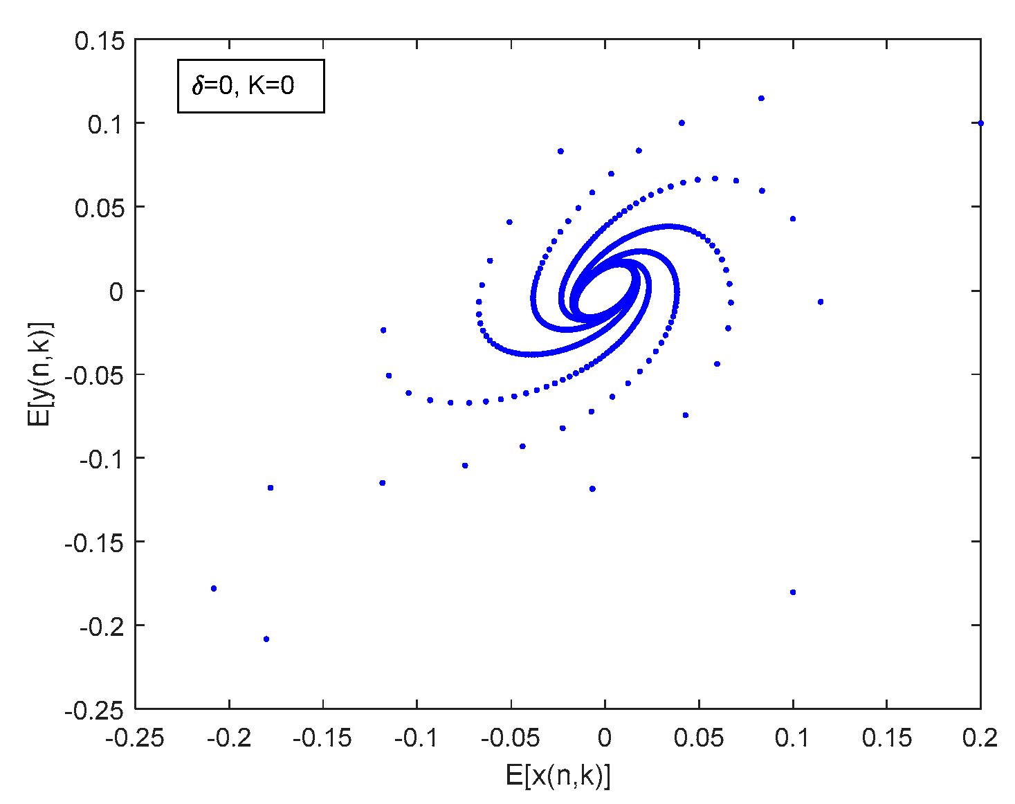
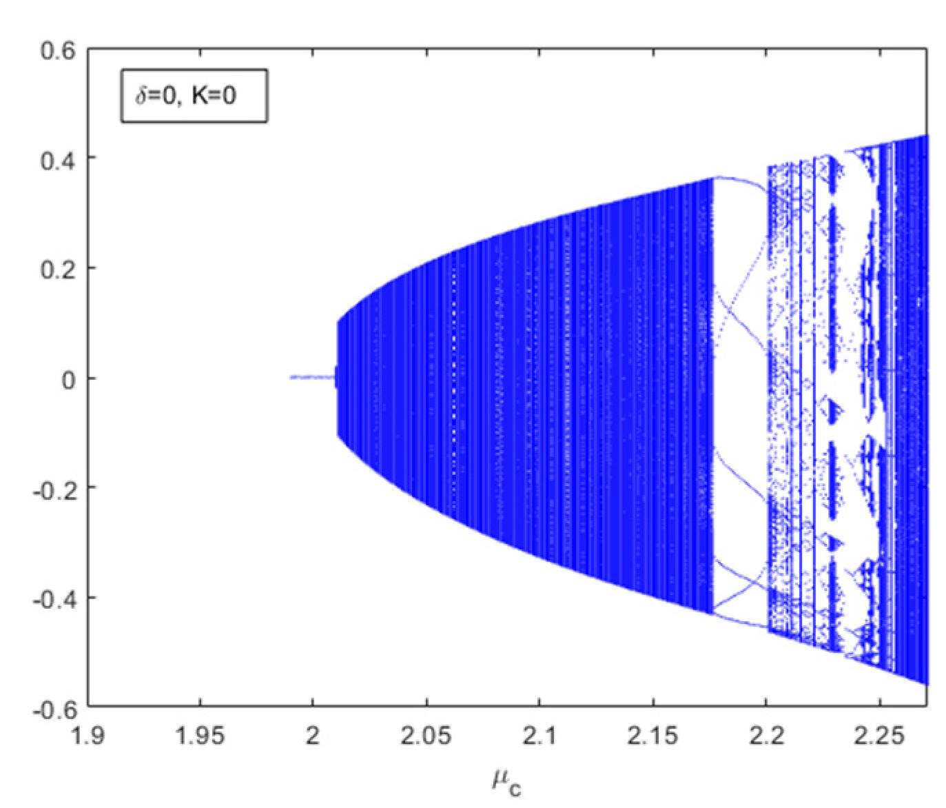
Let intensity $\delta =0,$ control coefficient $K=0,$ namely, the system is free from interference and control, so that the stochastic lagged discrete ecosystems (2) can be degenerated to a deterministic original lagged discrete ecosystem. The phase trajectory diagram and the bifurcation diagram of the ecosystem are shown in Figure 1 and Figure 2, respectively.

It can be seen from Figure 1 that the system has abundant dynamic behaviors, such as bifurcation and chaos. Figure 2 shows the bifurcation phenomenon at an equilibrium point. This shows that the ecosystem is unstable, so it is of great practical significance to control and disturb the ecosystem.

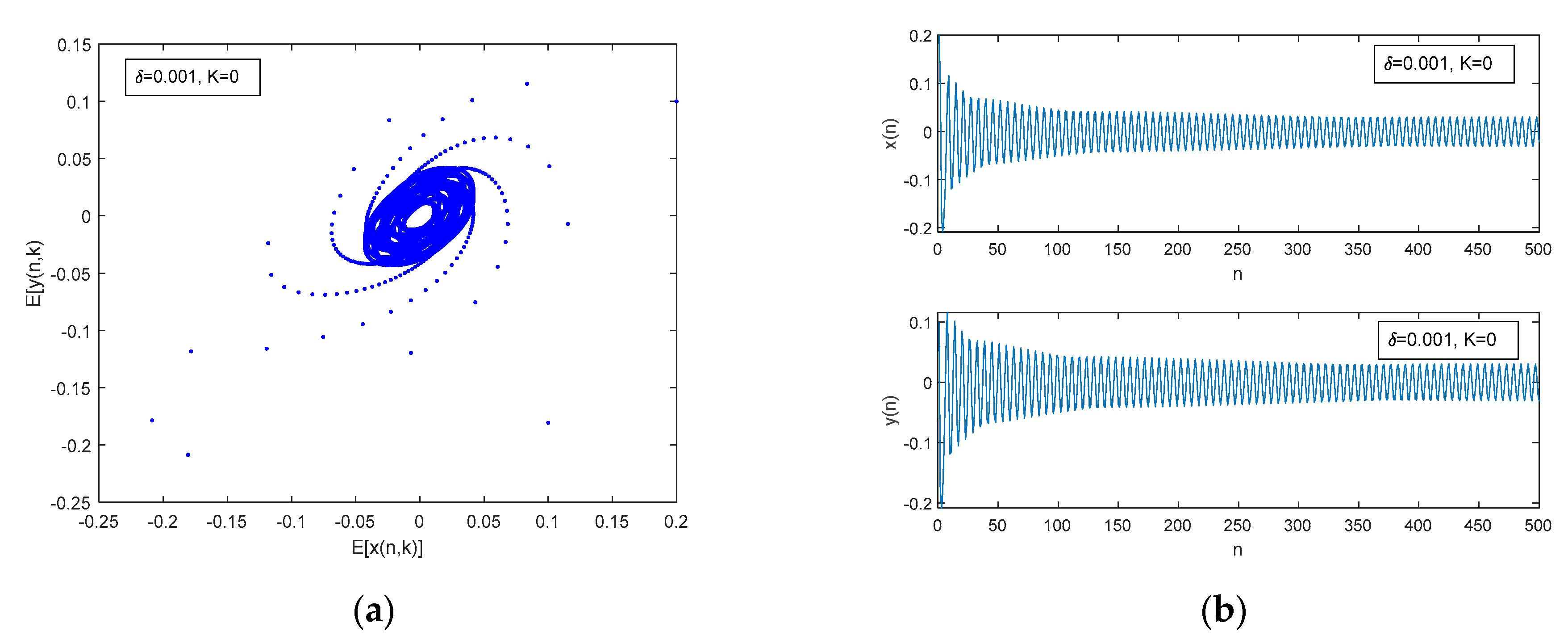
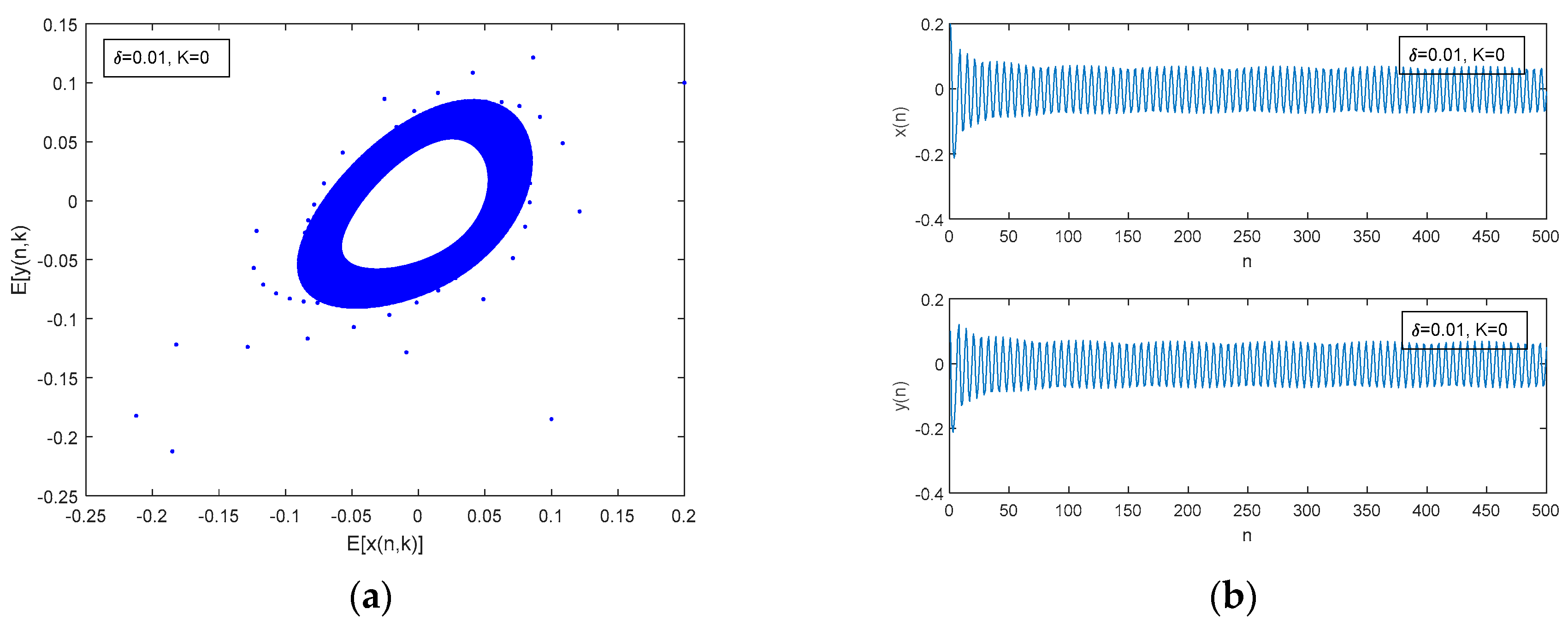
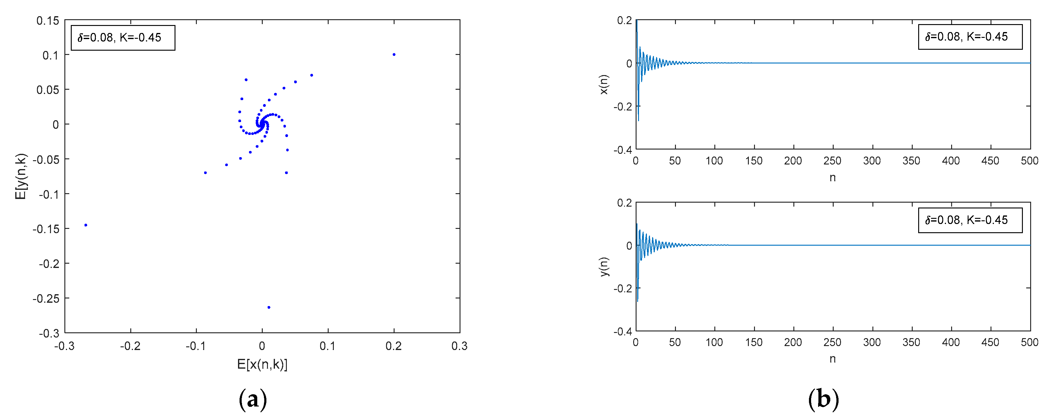
Because the intensity of $\delta$ is very small, when intensity $\delta =0.001,K=0$, phase trajectories and the time history diagrams of EMR of equivalent system (12) gradually converge to zero in Figure 2 and Figure 3a. We know that the stochastic lagged discrete ecosystem occurs bifurcation, which is shown by Figure 2. When $\delta =0.01,K=0$, the phase trajectories and time history diagrams of (12) that converge a limit cycle is shown in Figure 4. When the random intensity $\delta =0.05,K=0$, the system limits cycle amplitude increases are shown in Figure 5. From Figure 2, Figure 3, Figure 4, Figure 5and Figure 6, under the condition that the system is not controlled, it can be seen that the system limit loop increases as the stochastic intensity continues to increase, which also indicates that the intensity of external perturbations affects the stochastic lagged ecosystem dynamic behavior. It affects the stability of the ecosystem and places the equilibrium point of the system in an unstable state.

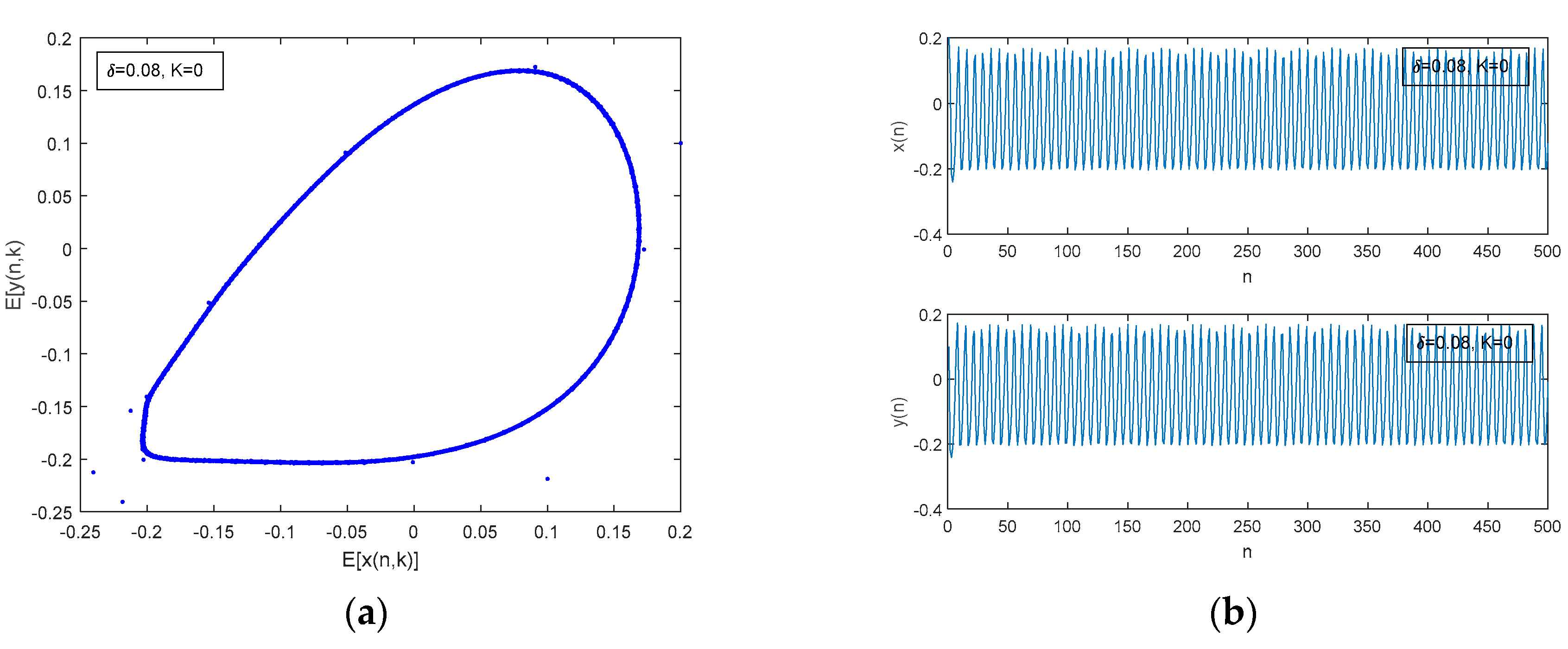
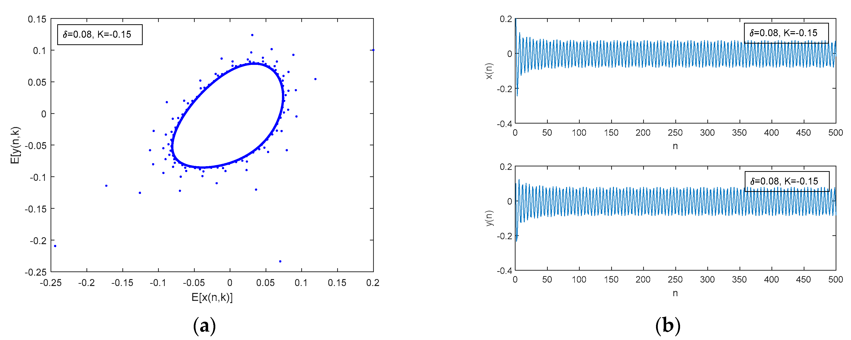
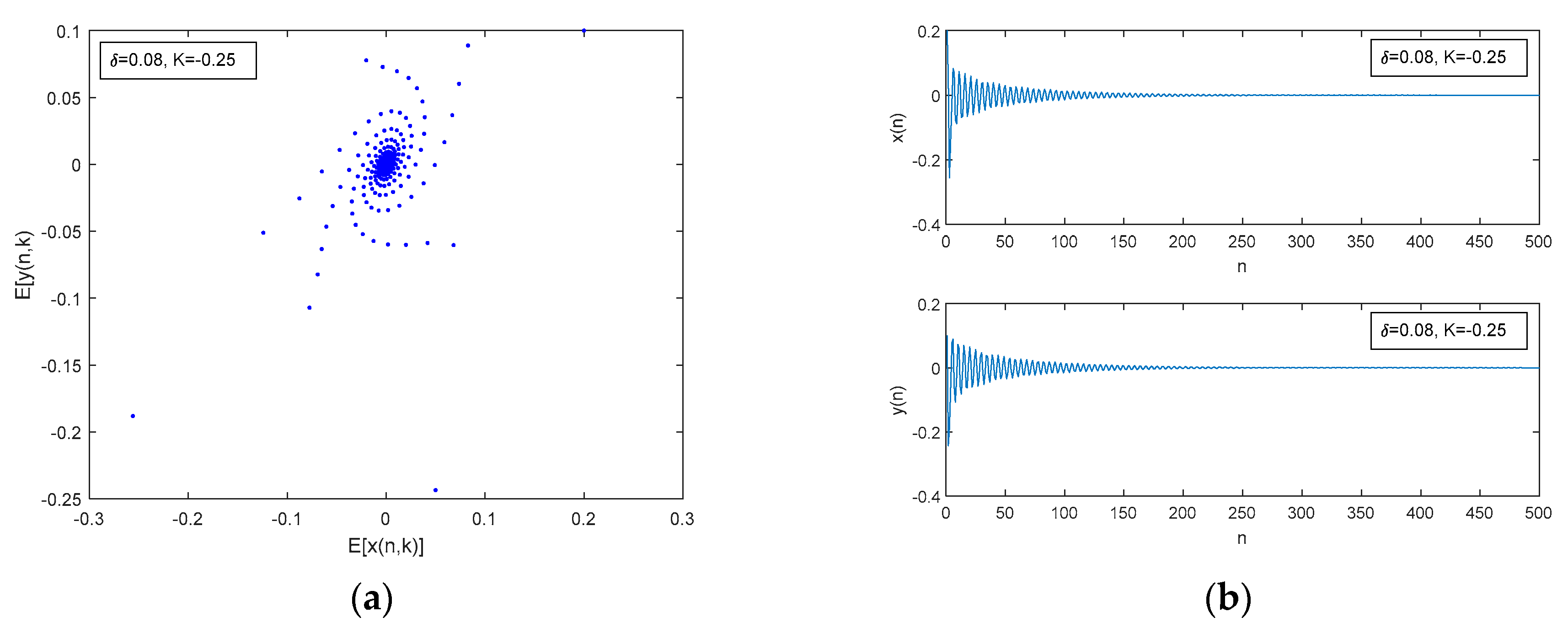
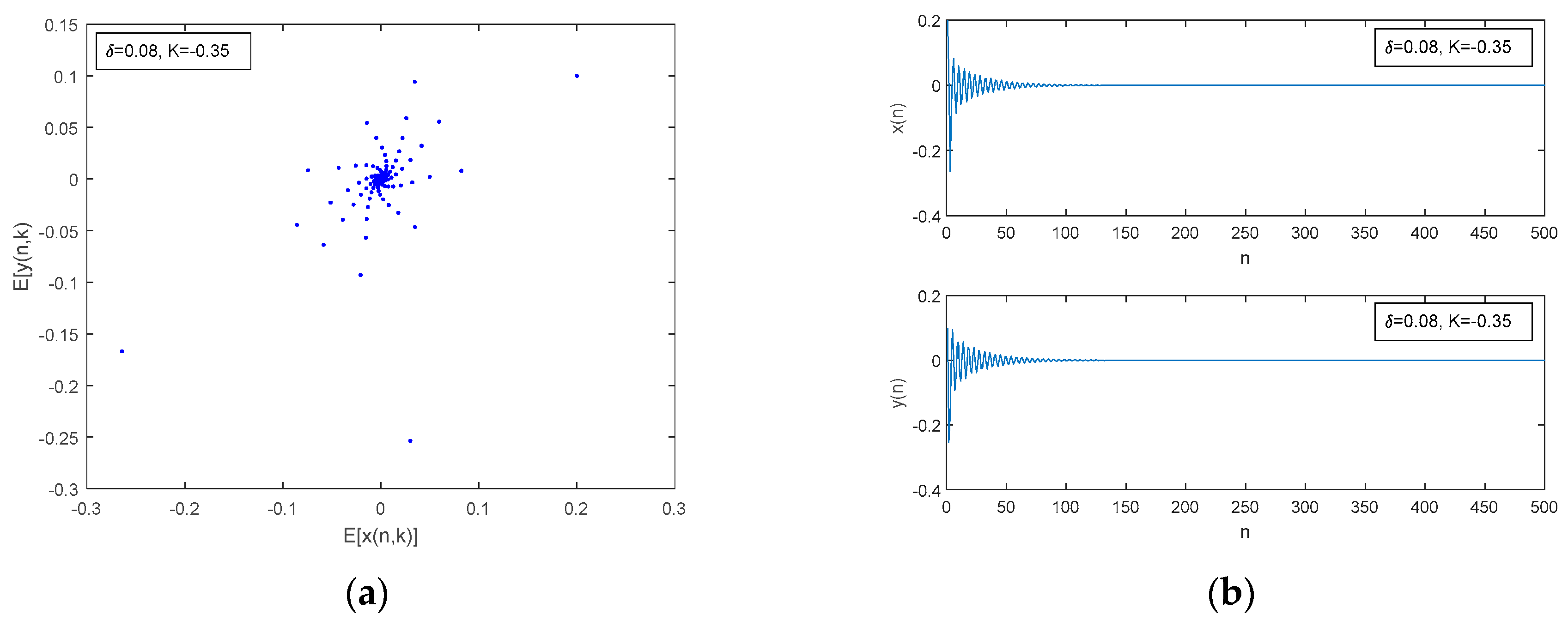
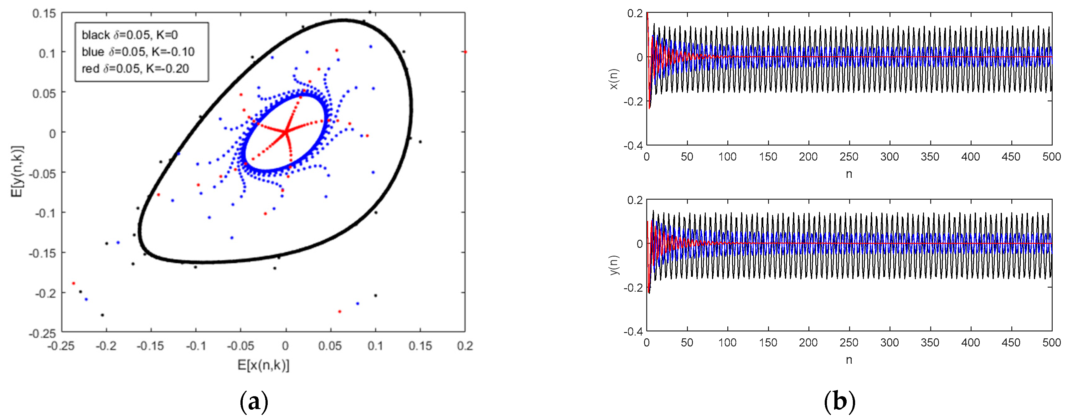
When random intensity $\delta =0.08$ and control coefficient $K=-0.15$, the limit cycle amplitude of the ecosystem is significantly smaller than that of the system without control by Figure 7 with phase portrait (a) and time history diagram (b). Starting from Figure 7, Figure 8, Figure 9 and Figure 10, the designed control function is constantly changing; specifically, the control coefficient is gradually changing, i.e., impose controls on the ecosystem, we will find that the bifurcation of the random lag ecosystem is controlled, leaving the ecosystem in a stable state.

Apparently, in Figure 6, Figure 7, Figure 8, Figure 9 and Figure 10, the control functions of stochastic lagged discrete ecosystem satisfy the control function conditions involved in Theorem 1 and Theorem 2. We obtain that the asymptotic stability and Hopf bifurcation in the stochastic lagged discrete ecosystem varies from random intensity and control functions by the numerical analysis. At the same time, it is also confirmed that the control function designed by us can control the dynamic behavior of the discrete ecosystem with random lag and make the system reach a stable state.

Next, Figure 11 shows the above design of the control function of random delay discrete control effect of the ecosystem, we will find that the system with the limit cycle amplitude control function coefficient decreases gradually, until a steady state is reached, such as the red part of the phase diagram (a), and the time history diagram (b) refers to a stable state.

According to theoretical analysis and numerical simulation, we have shown stochastic lagged discrete ecosystem stability with the variety of control functions. Obviously, comparing to the deterministic system, random intensity affects the dynamic behavior of its stochastic system, and the system bifurcation limit ring amplitude increases with the random intensity. However, we have designed control functions that control the asymptotic stability and bifurcation behavior of stochastic time-lag discrete ecosystems until the system reaches a steady state.

4. Conclusions

Using the orthogonal polynomial approximation theory of discrete random function, it is possible to study the control analysis of stochastic lagged discrete ecosystem. We successfully simplified the stochastic lagged discrete ecosystem to its equivalent deterministic system. The stability theory of deterministic systems and Hopf bifurcation theory, a control function is drawn up and control conditions for system stability are derived. Theoretical results are verified by numerical simulation and numerical analysis.

References

- Parrott, L. Measuring ecological complexity. Ecol. Indic. 2010, 10, 1069–1076. [Google Scholar] [CrossRef]
- Goldenberg, S.U.; Nagelkerken, I.; Marangon, E.; Bonnet, A.; Ferreira, C.M.; Connell, S.D. Ecological complexity buffers the impacts of future climate on marine consumers. Nat. Clim. Chang. 2018, 8, 229–233. [Google Scholar] [CrossRef]
- Farina, A. Ecoacoustic codes and ecological complexity. Biosystems 2018, 164, 147–154. [Google Scholar] [CrossRef] [PubMed]
- Liu, Q.K.; Zhang, Z.J.; Chen, X.M.; Li, Y.H. Stability Analysis of Enterprises Competition Based on Ecological Model. Math. Pract. Theory 2016, 46, 1–7. [Google Scholar]
- Chen, X.X.; Song, G.H.; Wang, X.J.; Li, Z.Y. Stability and Hopf Bifurcation of a Kind of Pinus Koraiensis Ecological System with Time Delay. J. Biomath. 2014, 29, 577–585. [Google Scholar]
- Jiang, H.B.; Li, X.Z.-P. Bifurcation Analysis of Complex Behavior in the Logistic Map via Periodic Impulsive Force. Acta Phys. Sin. 2013, 62, 120508. [Google Scholar] [CrossRef]
- Zan, Q.T. Study on the Complicated Dynamical Behaviors of Nonlinear Ecosystem. Appl. Math. Mech. 1988, 9, 925–931. [Google Scholar]
- Niu, S.Y.; Jin, Y.F. Stability Analysis of a Stochastic Predator-Prey Model with Harrison Function Response. J. Dyn. Control 2016, 14, 276–282. [Google Scholar]
- Li, D.M.; Ma, Z.F. Looking to the Future of Mathematical Ecology and Ecological Modelling. Acta Ecol. Sin. 2000, 20, 1083–1089. [Google Scholar]
- May, R.M. Simple Mathematical Models with Very Complicated Dynamics. Nature 1976, 261, 459–467. [Google Scholar] [CrossRef]
- Wang, Y.; Zhao, M.; Yu, H.; Dai, C.; Mei, D.; Wang, Q.; Ma, Z. Analysis of spatiotemporal dynamic and bifurcation in a wetland ecosystem. Discret. Dyn. Nat. Soc. 2015, 2015, 185432. [Google Scholar] [CrossRef]
- Liu, X.; Zhu, Q. Stochastically globally exponential stability of stochastic impulsive differential systems with discrete and infinite distributed delays based on vector Lyapunov function. Complexity 2022, 2020, 7913050. [Google Scholar] [CrossRef]
- Chen, L.Q.; Liu, Z.R. Control of a hyperchaotic discrete system. Appl. Math. Mech. 2001, 22, 741–746. [Google Scholar] [CrossRef]
- Tie, L.; Lin, Y. On controllability of two-dimensional discrete-time bilinear systems. Int. J. Syst. Sci. 2015, 46, 1741–1751. [Google Scholar] [CrossRef]
- Ahmed, A. On the stability of two-dimensional discrete systems. IEEE Trans. Autom. Control 1980, 25, 551–552. [Google Scholar] [CrossRef]
- Ooba, T. Asymptotic stability of two-dimensional discrete systems with saturation nonlinearities. IEEE Trans. Circuits Syst. I Regul. Pap. 2012, 60, 178–188. [Google Scholar] [CrossRef]
- Jia, W.; Xu, Y.; Li, D. Stochastic dynamics of a time-delayed ecosystem driven by Poisson white noise excitation. Entropy 2018, 20, 143. [Google Scholar] [CrossRef] [Green Version]
- Wan, K. Iterative learning control of two-dimensional discrete systems in General model. Nonlinear Dyn. 2021, 104, 1315–1327. [Google Scholar] [CrossRef]
- Wang, X.Y.; Luo, C. Dynamic analysis of the coupled logistic map. J. Softw. 2006, 17, 729–739. [Google Scholar] [CrossRef] [Green Version]
- Zong, X.P.; Geng, J.; Wang, P. Bifurcation Control of the Coupled Logistic Mapping. Inf. Control 2011, 40, 343–351. [Google Scholar]
- Wang, X.Y.; Wang, M.J. Chaos control of two-dimensional Logistic mapping. Acta Phys. Sin. 2008, 57, 731–736. [Google Scholar]
- He, Z.M.; Lai, X. Bifurcation and chaotic behavior of a discrete-time predator-prey system. Nonlinear Anal. Real World Appl. 2011, 12, 403–417. [Google Scholar] [CrossRef]
- Chen, S.S.; Shi, J.P. Stability and Hopf bifurcation in a diffusive logistic population model with non local delay effect. J. Differ. Equ. 2012, 253, 3440–3470. [Google Scholar] [CrossRef] [Green Version]
- Song, Y.L.; Peng, Y.H. Stability and bifurcation analysis on a logistic model with discrete and distributed delays. Appl. Math. Comput. 2006, 181, 1745–1757. [Google Scholar] [CrossRef]
- Feng, T.; Meng, X.Z. Stochastic Dynamics of a Predator-prey System with Disease in Predator. J. Shandong Univ. Sci. Technol. 2017, 36, 99–110. [Google Scholar]
- Ma, S.J.; Dong, D. The Asymptotic Stability Analysis in Stochastic Logistic Model with Poisson Growth Coefficient. Theor. Appl. Mech. Lett. 2014, 4, 0130041–0130049. [Google Scholar] [CrossRef] [Green Version]
- Liu, Y.; Liu, Q.; Liu, Z. Dynamical Behaviors of a Stochastic Delay Logistic System with Impulsive Toxicant Input in a Polluted Environment. J. Theor. Biol. 2013, 329, 1–5. [Google Scholar] [CrossRef]
- Ma, S.J.; Dong, D.; Zheng, J. Generalized Synchronization of Stochastic Discrete Chaotic System with Poisson Distribution Coefficient. Discret. Dyn. Nat. Soc. 2013, 2013, 981503. [Google Scholar] [CrossRef]
- Ma, S.J.; Dong, D.; Yang, M.S. Stochastic Hopf bifurcation analysis in a stochastic lagged logistic discrete-time system with Poisson distribution coefficient. Nonlinear Dyn. 2015, 80, 269–279. [Google Scholar] [CrossRef]
- Elaydi, S. An Introduction to Difference Equations, 3rd ed.; Springer: Berlin/Heidelberg, Germany, 2005. [Google Scholar]
- Wen, G.L. Criterion to identify Hopf bifurcations in maps of arbitrary dimension. Phys. Rev. E 2005, 72, 026201. [Google Scholar] [CrossRef]
Figure 1.
The phase trajectory diagram of ecosystems.
Figure 2.
The bifurcation diagram of ecosystems.
Figure 3.
Phase portrait (a) and time history diagram (b) for .
Figure 4.
Figure 5.
Figure 6.
Figure 7.
Figure 8.
Figure 9.
Figure 10.
Figure 11.
Publisher’s Note: MDPI stays neutral with regard to jurisdictional claims in published maps and institutional affiliations. |
© 2022 by the author. Licensee MDPI, Basel, Switzerland. This article is an open access article distributed under the terms and conditions of the Creative Commons Attribution (CC BY) license (https://creativecommons.org/licenses/by/4.0/).
Share and Cite
MDPI and ACS Style
Zhang, J. Control Analysis of Stochastic Lagging Discrete Ecosystems. Symmetry 2022, 14, 1039. https://0-doi-org.brum.beds.ac.uk/10.3390/sym14051039
AMA Style
Zhang J. Control Analysis of Stochastic Lagging Discrete Ecosystems. Symmetry. 2022; 14(5):1039. https://0-doi-org.brum.beds.ac.uk/10.3390/sym14051039
Chicago/Turabian StyleZhang, Jinyi. 2022. "Control Analysis of Stochastic Lagging Discrete Ecosystems" Symmetry 14, no. 5: 1039. https://0-doi-org.brum.beds.ac.uk/10.3390/sym14051039
Note that from the first issue of 2016, this journal uses article numbers instead of page numbers. See further details here.