How a Nonequilibrium Bath and a Potential Well Lead to Broken Time-Reversal Symmetry—First-Order Corrections on Fluctuation–Dissipation Relations

Abstract

The noise that is associated with nonequilibrium processes commonly features more outliers and is therefore often taken to be Lévy noise. For a Langevin particle that is subjected to Lévy noise, the kicksizes are drawn not from a Gaussian distribution, but from an $\alpha$-stable distribution. For a Gaussian-noise-subjected particle in a potential well, microscopic reversibility applies. However, it appears that the time-reversal-symmetry is broken for a Lévy-noise-subjected particle in a potential well. Major obstacles in the analysis of Langevin equations with Lévy noise are the lack of simple analytic formulae and the infinite variance of the $\alpha$-stable distribution. We propose a measure for the violation of time-reversal symmetry, and we present a procedure in which this measure is central to a controlled imposing of time-reversal asymmetry. The procedure leads to behavior that mimics much of the effects of Lévy noise. Our imposing of such nonequilibrium leads to concise analytic formulae and does not yield any divergent variances. Most importantly, the theory leads to simple corrections on the Fluctuation–Dissipation Relation.

1. Introduction

The Fluctuation–Dissipation Relation (FDR) is as simple as it is profound [1]. For a particle in a fluid we have

$$D/\left(k_{B}T\right)=\mu .$$

(1)

On the left-hand side of this equation, D is the diffusion coefficient of the particle, $k_B$ is Boltzmann’s constant, and T is the absolute temperature. The product $k_{B}T$ has the dimension of energy and it is the characteristic “quantum” of Brownian motion. On the right-hand side, $\mu$ denotes the mobility, i.e., $\mu =v/F$ where v is the average speed of the particle in the fluid when it is subjected to a force F.

On the molecular level, there are other manifestations of the FDR. Take a resistor with a conductance G. With no net current flowing, there is still a fluctuating voltage between the two ends of the resistor due to the Brownian motion of the charge carriers (generally electrons) inside the resistor. Conductance can be viewed as the electrical equivalent of mobility, i.e., $G=I/V$, with V being the voltage and I being the current. With this realization, it is not hard to understand that the mean square of the fluctuating current, $\langle I^2\rangle$, is related to the conductance G through $k_{B}T$. The relation $\langle I^2\rangle =4k_{B}TG(\Delta f)$, where $\Delta f$ is the frequency window, is known as the Johnson–Nyquist relation [2].

Thinking of it more abstractly, the FDR connects characteristics of internal fluctuations on the left-hand side of Equation (1) with a first-order, linear response to external prompting on the right-hand side of Equation (1). The equation relates the first moment upon application of a perturbing force to the second moment in the absence of such a force. A more all-encompassing formulation of the FDR is due to Green and Kubo [3].

For the FDR to apply, it is essential that the system is close to equilibrium. Equilibrium means that there is no identifiable arrow of time. A system at equilibrium displays time-reversal symmetry. About a century ago, Lars Onsager formulated the notion of microscopic reversibility, which is short for “time reversibility of microscopic dynamics” [4,5]. It means that any trajectory in a configuration space from an initial point $(t_{ini},x_{ini})$ to a final point $(t_{fin},x_{fin})$ is traversed in one direction as often as it is in the opposite direction. Much of the first-order theory that describes systems that are close to equilibrium, such as Onsager’s reciprocal relation for coupled energy flows, is based on the idea that microscopic reversibility still applies in case of small deviation from equilibrium [4,5].

Considerable research effort has been directed towards formulating an FDR for a system that is far away from equilibrium. In the late 1990s, the Jarzynski Equation gave insight into the response of a system when nonequilibrium is imposed beyond a regime where linear perturbation theory applies [6,7]. The Jarzynski Equality has an elegant simplicity, and soon after its discovery, it also turned out remarkably accurate in quantitatively accounting for the results of micromanipulation experiments with biomolecules [8].

The work towards a nonequilibrium FDR has commonly taken an approach that is similar to the one that led to the Jarzynski Equation [9,10]. The guiding idea has been to let nonequilibrium events happen in a bath that is at equilibrium and that has a temperature. Temperature is a collective property and actually only makes sense if the collective is at equilibrium.

But what if the bath is the very source of nonequilibrium?

In liquid water at room temperature, an individual water molecule collides about ${10}^{12}$ times per second. For time intervals $\Delta t$ that are significantly larger than a picosecond, the displacement of such a water molecule is the result of many collisions. The Central Limit Theorem [1] applies in that case, and the displacement in $\Delta t$ follows the Gaussian distribution that is associated with equilibrium.

Through numerical simulation, Kanazawa et al. recently showed that in active media, i.e., media with artificial self-propelled colloids or swimming microorganisms, displacements of passive tracers follow not a Gaussian, but an $\alpha$-stable distribution [11].

Where a Gaussian distribution results for a process that is the cumulative effect of stochastic processes with a finite standard deviation, an $\alpha$-stable distribution results when infinite standard deviations come into play. The analytic expression for the $\alpha$-stable distribution is huge and cumbersome, but in Fourier space, a concise formula ensues. For a symmetric, zero-centered $\alpha$-stable distribution, the generating function is:

$${\tilde{p}}_{\alpha }\left(k\right)=exp\left[-c^{\alpha }{\left|k\right|}^{\alpha }\right].$$

(2)

Here, c is a scale factor and $\alpha$ is the so-called stability index ($0<\alpha \le 2$). For $\alpha =2$, the Gaussian distribution is actually retrieved and for $\alpha =1$, the $\alpha$-stable distribution is the simple and well-known Cauchy distribution, i.e., $p\left(x\right)=(c/\pi ){(c^2+x^2)}^{-1}$.

Nonequilibrium is commonly characterized by frequently occurring “outliers” [12,13,14,15,16,17]. If “outliers” means a Brownian trajectory with an overabundance of very large steps, then replacing the Gaussian distribution by an $\alpha$-stable distribution is the next sensible move in the modeling.

It is in the asymptotics, i.e., the behavior at $\left|x\right|\to \infty$, that we find the most salient difference between a Gaussian and an $\alpha$-stable distribution. For the Gaussian distribution, the convergence follows $p\left(x\right)\sim exp\left[-x^2/4c^2\right]$ and is rapid (note here that for $\alpha =2$, the scale factor c is the standard deviation divided by $\sqrt{2}$). For the $\alpha$-stable distribution, the tail follows a power law: $p\left(x\right)\sim {\left|x\right|}^{-\alpha -1}$. The slow convergence of the power-law tail leads to an infinite standard deviation and is also behind the more frequent occurrence of outliers [18,19].

2. Overdamped Particle in a Potential Well Subjected to IID $\mathbf{\alpha }$-Stable Noise

Consider a particle in a potential $V\left(x\right)$ that is subjected to $\alpha$-stable noise. We have for the Langevin Equation for the position $x\left(t\right)$ of an overdamped particle:

$$\beta \dot{x}=-\frac{dV\left(x\right)}{dx}+\beta c{\xi }_{\alpha }\left(t\right).$$

(3)

In the course of a simulation with timesteps of length $\Delta t$, a noise contribution $\xi \left(t_i\right)$ at the i-th step is taken as ${\xi }_{\alpha }\left(t_i\right)={\theta }_{\alpha ,i}\Delta t^{1/\alpha -1}$, where ${\theta }_{\alpha ,i}$ is the i-th random number in the sequence of steps. The random numbers ${\theta }_{i,\alpha }$ are drawn from an $\alpha$-stable distribution with a scale factor of one. They are independent and identically distributed (IID). The $1/\alpha$ in the exponent of $\Delta t$ guarantees that the diffused distance scales correctly if different $\Delta t$’s are taken. Equation (3) furthermore shows how the scale factor is effectively an amplitude. For Gaussian noise, i.e., $\alpha =2$, the scale factor c is the usual $\sqrt{2D}$, where D is the diffusion coefficient. The variable $\beta$ denotes the coefficient of friction. The coefficient of friction is the inverse of the aforementioned mobility $\mu$, i.e., $\beta =1/\mu$. The left- and right-hand sides of Equation (3) have the dimension of force. We consider a small segment of a trajectory going from $(t_i,x_i)$ to $(t_i+\Delta t,x_i+\Delta x_i)$. Multiplying with $\Delta x_i$, we obtain the involved energies: $\beta \left(\frac{\Delta x_i}{\Delta t}\right)\Delta x_i=\left[F\left(x_i\right)+\beta c{\xi }_{\alpha }\left(t_i\right)\right](\Delta x_i)$. Here, the term on the left-hand side indicates the amount of energy that is “dissipated out” in time $\Delta t$. The term in square brackets on the right-hand side denotes the net force on the particle. The net force is made up of the force due to the potential, $F\left(x_i\right)=-dV\left(x_i\right)/dx$, and the force due to agitation by the bath. Multiplying the net force by the distance $\Delta x_i$ over which the force is applied, we obtain the work performed on the particle over the segment $\Delta x_i$. Writing $F\left(x_i\right)\Delta x_i=-V\left(x\right){|}_{x_i}^{x_{i+1}}$, substituting $\Delta x_i=\left[F\left(x_i\right)/\beta +c{\xi }_{\alpha }\left(t_i\right)\right]\Delta t$ on the right-hand side, and using ${\xi }_{\alpha }\left(t_i\right)={\theta }_{\alpha ,i}\Delta t^{1/\alpha -1}$ again, we find:

$$\beta \frac{{\left(\Delta x_i\right)}^2}{\Delta t}{+V\left(x\right)|}_{x_i}^{x_{i+1}}=cF\left(x_i\right){\theta }_{\alpha ,i}\Delta t^{1/\alpha -1}+\beta c^2{\theta }_{\alpha ,i}^2\Delta t^{2/\alpha -1}.$$

(4)

This equation again describes the energy traffic for the particle in a time interval $\Delta t$. On the left-hand side, the first term is the dissipated energy and the second term is the energy associated with going up or down in the potential. The twofold expression on the right-hand side describes the energy that is “fluctuated into the particle.” The second term would be the only contribution in case of a flat potential. The first term accounts for the interplay between the random kicks, ${\xi }_{\alpha }\left(t_i\right)$, and the deterministic $F\left(x_i\right)$. If the Brownian kick and the deterministic force are in the opposite direction and such that they balance each other out, then the right-hand-side terms in Equation (4) will add up to zero and the particle will not move.

For the case of $\alpha =2$, Equation (4) readily reduces to something more familiar. On the left-hand side, the existence of a basin of attraction implies that the changes ${V\left(x\right)|}_{x_i}^{x_{i+1}}$ will ultimately average to zero. Furthermore, we have $\langle {\theta }_{2,i}\rangle =0$ and $\langle F\left(x_i\right)\rangle =0$ in this case. As the kicksizes ${\theta }_{2,i}$ are not correlated to $F\left(x_i\right)$, we also have $\langle F\left(x_i\right){\theta }_{2,i}\rangle =0$ on the right-hand-side. The Gaussian case, $\alpha =2$, also leads to $\langle {\theta }_{2,i}^2\rangle =1$. With $c^2=2D$ and invoking the FDR, $\beta D=k_{B}T$, we then obtain:

$$\beta \langle {\dot{x}}^2\rangle =\frac{2k_{B}T}{\Delta t}.$$

(5)

This equation tells us that the long-time average of the energy that is fluctuated into the particle is $2k_{B}T$ per timestep. Note that in the continuum limit, $\Delta t\to 0$, an infinite amount of energy flows through each particle in the system in any finite amount of time. The Langevin Equation, however, is an abstraction. As was mentioned before, in actual reality there is about a picosecond between subsequent collisions of an individual water molecule, and this puts a lower limit on the value of $\Delta t$. Equation (5) has proven fruitful in the analysis of Brownian ratchets [20,21].

A lot more infinities start accumulating once we make $\alpha <2$. For $0<\alpha <2$, the variance $\langle {\theta }_{\alpha ,i}^2\rangle$ diverges. Effectively, this means that the bath has no temperature. No FDR can be formulated in this case. For $0<\alpha \le 1$, $\langle {\theta }_{\alpha ,i}\rangle$ is zero-centered, but does not converge. This leads to further problems in working with Equation (4). However, most real-life instances of Lévy noise involve values of $\alpha$ that are between 1 and 2 [12,13,14,15,16,17].

Below we propose a way to “fix” the $\langle {\theta }_{\alpha ,i}^2\rangle$-divergence for small deviations from equilibrium. The idea is inspired by the violation of time-reversal symmetry that Lévy noise causes for a particle in a potential well. We will derive some simple formulae that we will check against the results of numerical simulation.

3. Nonequilibrium and Time-Reversal Asymmetry in a Parabolic Well

If $V\left(x\right)$ is a flat potential, then Equation (3) describes a simple 1D random walk. Both for $\alpha =2$ and $\alpha \ne 2$, we then have time-reversal symmetry. If one were to make a movie of the moving particle, it would afterwards not be possible to determine whether the movie is played forward or backward. However, when the Brownian particle is in a 1D potential well, a different situation arises. When subjected to white Gaussian noise, Onsager’s microscopic reversibility has to apply, i.e., we still have time-reversal symmetry. When, on the other hand, the particle in the 1D potential well is subjected to Lévy noise, time-reversal symmetry is violated. Below, we will explain this violation and elaborate on it. Based on the developed insights, we will formulate a measure for the time-reversal-symmetry breaking and we will derive approximate FDR relations for a nonequilibrium bath.

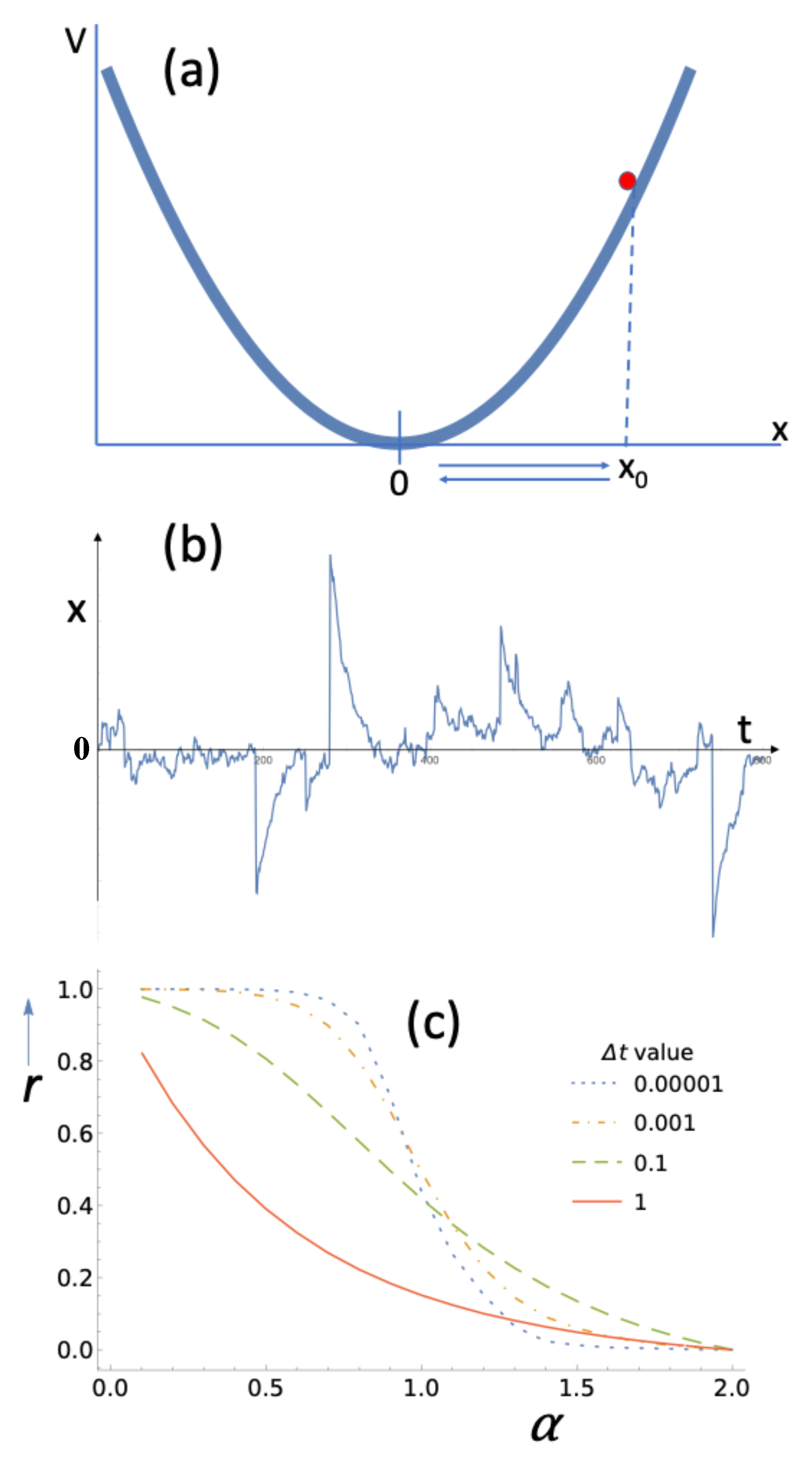
Consider the situation with the parabolic well, $V\left(x\right)=\frac{1}{2}A{x}^2$ with $A>0$, as depicted in Figure 1a. Let the Brownian fluctuations make the particle go up the parabola to a considerable height $x_0$ outside the basin of attraction. As the basin of attraction of the potential, we take the interval around the minimum where the particle spends around 90% of its time. In case of Gaussian noise, we have microscopic reversibility. The most likely Brownian kick has a magnitude of zero. Therefore, the most likely downslide is a series of such “zero” kicks and the most likely upslide is, perhaps unintuitively, the exact reverse. The deterministic downslide follows $\beta \dot{x}=-Ax$. This leads to $x\left(t\right)=x_{0}exp\left[-At/\beta \right]$. If we let the downslide run from $x_0$ all the way back back to $x=0$, then we have for the dissipated energy $\int \beta \dot{x}\left(t\right)dx\left(t\right)=\beta {\int }_0^{\infty }{\dot{x}}^{2}dt=({\beta }^2/\left(2A\right))x_0^2$. In principle, the downslide to $x=0$ takes infinitely long. However, if we take as the endpoint a location $x_{*}$ in the basin of attraction, then we have for the time $t_{*}$ to reach $x_{*}$: $t_{*}=\beta log\left[x_0/x_{*}\right]/A$. With a discretized time, this corresponds to $n=t_{*}/(\Delta t)=(\beta log\left[x_0/x_{*}\right])/(A\Delta t)$ timesteps.

With Gaussian noise, the most likely upslide and most likely downslide both take n steps. In Ref. [22], it is shown rigorously that in case of Lévy noise, the most likely upslide takes one step and the most likely downslide takes n steps. Reference [22], furthermore, works out the case of $\alpha =1$ (when the $\alpha$-stable distribution is actually the Cauchy distribution) in great detail. Given what is observed in Figure 1b, it is not hard to intuit the apparent violation of time-reversal symmetry. The noisy particle will spend most of its time in the basin of attraction near the bottom of the well. A Lévy jump makes the particle “shoot up” in one step. Afterwards, it will slide down as if in equilibrium. Doing the upslide in one step (i.e., doing it n times as fast as the deterministic downslide) leads to the dissipation of n times as much energy. This can be readily seen from the integral that gives the dissipated energy: $E_{diss}=\int \beta \dot{x}\left(t\right)dx\left(t\right)$.

Figure 1b affirms the insight formulated in the previous paragraph. The one-step Lévy jumps are conspicuous, and so are the slower subsequent relaxations back to the bottom of the well.

For a potential with curvature, there is a problem when simulating the motion of a particle that is subjected to Lévy noise. Imagine that the particle in Figure 1a is to the left of $x=0$, and imagine next that it receives a large Lévy kick to the right. In a simple Euler scheme with a timestep $\Delta t$, we would have the deterministic force on the particle, $F\left(x\right)=-dV\left(x\right)/dx$, be in the positive direction for the entire interval, even when the particle is actually “climbing” the potential on the part of the potential where $x>0$. For a parabolic potential, the solution to this “large kick problem” is straightforward. Through scaling of t and x, the Langevin Equation $\beta \dot{x}=-Ax+\beta c{\xi }_{\alpha }\left(t\right)$ can be brought into a form $\dot{x}=-\lambda x+{\xi }_{\alpha }\left(t\right)$ [23]. We take $\lambda =1$. Upon discretization of $\dot{x}=-x+{\xi }_{\alpha }\left(t\right)$, we let the kick at $t=t_i$ have a value ${\xi }_{\alpha }\left(t_i\right)=K$. We then take the curvature of the potential into account by simply taking the solution of $\dot{x}=-x+K$ as describing what occurs between $x\left(t_i\right)=x_i$ and $x\left(t_{i+1}\right)=x_{i+1}$. This leads to $x_{i+1}=(x_i-K)e^{-\Delta t}+K$. Figure 1b,c was obtained using the latter expression at every timestep.

After taking the data from a computer simulation (with a time interval $\Delta t$) or from a real-life system (sampled at a time interval $\Delta t$), we can express the deviation from microscopic reversibility as follows:

$$r={\phi }_{\mathrm{desc}}-{\phi }_{\mathrm{asc}},$$

(6)

where ${\phi }_{\mathrm{desc}}$ and ${\phi }_{\mathrm{asc}}$ are the fraction of descending steps and the fraction of ascending steps, respectively. Descending steps are steps for which ${V\left(x\right)|}_{x_i}^{x_{i+1}}<0$ and ascending steps are steps for which ${V\left(x\right)|}_{x_i}^{x_{i+1}}>0$ (cf. Equation (4)). Time reversal turns ascending steps into descending steps and descending steps into ascending steps. So it is obvious that $r=0$ in case of microscopic reversibility. No arrow of time can exist at equilibrium and $r=0$ must ensue for any system at equilibrium. The parameter r indicates the level of symmetry breaking and can be thought of as an order parameter. Gaussian noise ($\alpha =2$) leads to $r=0$ on any shape potential, even if the potential is not a simple well.

Figure 1c shows r as a function of the stability index $\alpha$ for a Lévy-noise-subjected particle in a parabolic potential. Curves are drawn for different values of the time interval $\Delta t$. For Lévy noise, there is a power-law tail and a divergent variance for any $\alpha =2-\epsilon$, where $\epsilon$ is small and positive. For $\alpha =2$, the Gaussian is recovered. Nevertheless, the convergence to $r=0$ as $\alpha$ approaches 2 appears smooth.

From Figure 1c, it is also obvious that there is a strong dependence on the timestep $\Delta t$. It is for the green curve in Figure 1c, i.e., $\Delta t=0.1$, that we get the fastest departure from $r=0$. This apparent optimum is not hard to understand. In a parabola $V\left(x\right)=\frac{1}{2}A{x}^2$, the deterministic downslide starting at $x_0=x(t=0)$ is described by $x\left(t\right)=x_{0}exp\left[-At/\beta \right]$. In other words, there is a characteristic time $t_{\mathrm{char}}=\beta /A$ for the downslide. If $\Delta t\gg t_{\mathrm{char}}$, then the particle will generally be back in the basin of attraction after one timestep. The shooting up and sliding down will not be resolved in that case. Suppose next that $\Delta t\to 0^{+}$. With $\beta \Delta x_i=-A{x}_i\Delta t+\beta c{\theta }_i{(\Delta t)}^{1/\alpha }$ and $1<\alpha <2$, we then have $\Delta t^{1/\alpha }\gg \Delta t$. This leads to the noise-term being dominant and the contribution due to the slope being negligible. What this means in practice for the downslide is that it will take a very large number of steps, $N_{\mathrm{tot}}$, to get back to the basin of attraction after a Lévy jump. A number $N_{\mathrm{asc}}\approx N_{\mathrm{tot}}/2$ of these steps will be ascending and a number $N_{\mathrm{desc}}\approx N_{\mathrm{tot}}/2$ will be descending. The difference $N_{\mathrm{desc}}-N_{\mathrm{asc}}$ will be small relative to $N_{\mathrm{tot}}$ and will lead to $r=(N_{\mathrm{desc}}-N_{\mathrm{asc}})/N_{\mathrm{tot}}\to 0$. In between $\Delta t\to 0^{+}$ and $\Delta t\gg t_{\mathrm{char}}$ there will be a maximum for the value of r. Figure 1c shows that with a timestep, $\Delta t$, that is about one tenth of the characteristic time, $t_{\mathrm{char}}$, an optimal resolution of the nonequilibrium features is obtained. The parameter r for a Lévy particle in a harmonic potential is further explored in Ref. [23].

“… when all the fast things have happened, but the slow things have not.” That is how Richard Feynman once described equilibrium [24]. The observations in the previous paragraph on the Lévy particle’s relaxation to the basin of attraction put an interesting take on Feynman’s premise for the case of our nonequilibrium system. If we take $\Delta t\gg t_{\mathrm{char}}$, we are indeed not sampling sufficiently fast to see the relaxation happen and we are then looking at the $r=0$ that characterizes equilibrium. However, if we take $\Delta t\ll t_{\mathrm{char}}$, we are sampling too fast and also do not see the relaxation happen as sampling too fast likewise leads to $r=0$, i.e., the equilibrium result. So “… when the fast things happen, but we are sampling too fast to see it" would also describe equilibrium.

4. Corrections on the FDR for a Small Deviation from Microscopic Reversibility

As we saw earlier, with Gaussian noise, time-reversal symmetry implies that ascent and descent are, on average, equally fast. With Lévy noise, the most likely trajectory from the basin of attraction to a position $x_0$ high above the minimum takes one timestep. The subsequent most likely descent follows the deterministic pattern that would also ensue if there were equilibrium. Below, we analyze such breaking of time-reversal symmetry in a close-to-equilibrium condition. We will come to an intuitive understanding and associated approximate relations. Ultimately, we will derive how the FDR looks for a small deviation from equilibrium.

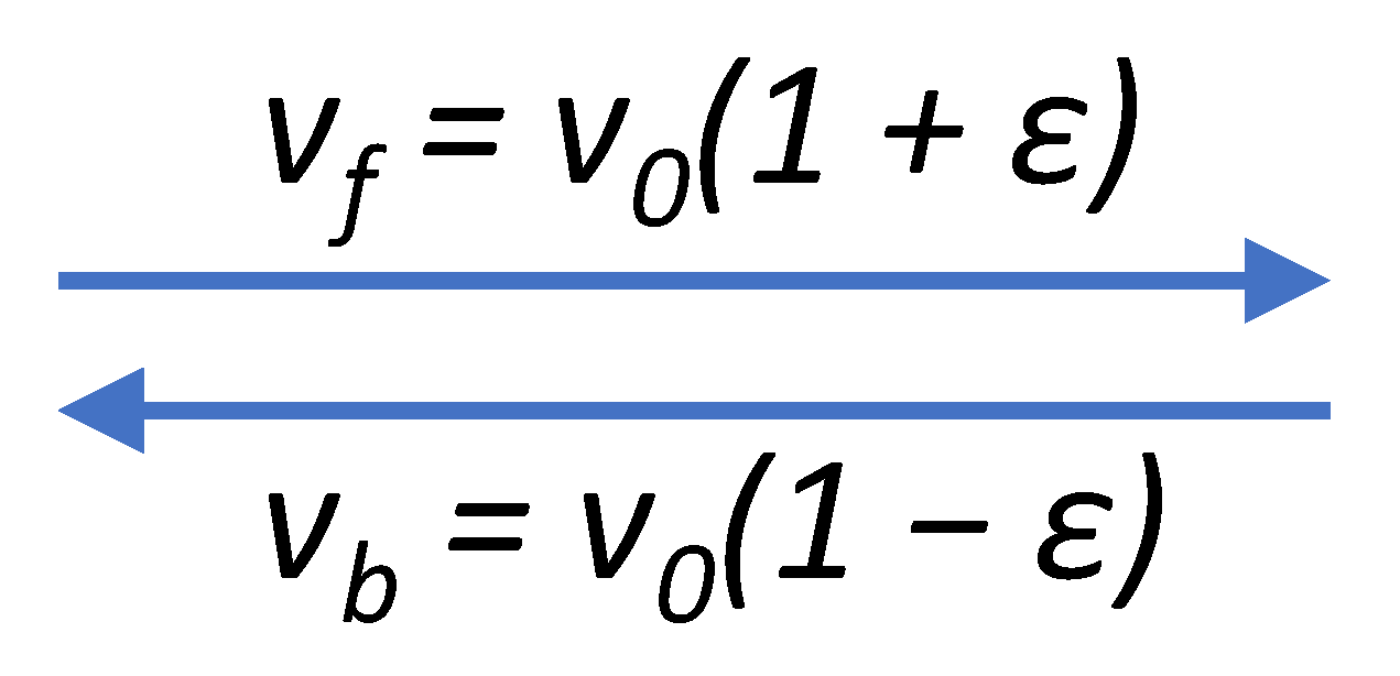
Consider a small interval $\Delta x_0$ on the x-axis. With a coefficient of friction $\beta$, the energy that is dissipated if $\Delta x_0$ is crossed at a speed v is $E=\beta v(\Delta x_0)$. Over a long time-interval, $\Delta x_0$ is traversed equally often in both directions. Let $v_0$ be the speed on the downslide and let $v_0(1+\delta )$ be the speed on the upslide. Close to equilibrium means that $\delta$ is sufficiently small to justify a first-order approximation. With the upslide speed corrected by a multiplicative factor $(1+\delta )$, the number of ascending steps gets a multiplicative factor $(1-\delta )$ relative to the number of descending steps. This leads to:

$$r=\frac{N_{\mathrm{desc}}-N_{\mathrm{asc}}}{N_{\mathrm{desc}}+N_{\mathrm{asc}}}=\frac{1-(1-\delta )}{1+(1-\delta )}\approx \frac{1}{2}\delta .$$

(7)

If $\Delta x_0$ is traversed first at an upslide-speed $v_0(1+\delta )$ and next, on the way back to the basin of attraction, at a speed $v_0$, then the dissipated energy is:

$$E_{\mathrm{diss}}^{\mathrm{noneq}}=\beta v_0(1+\delta )(\Delta x_0)+\beta v_0(\Delta x_0)=2\beta v_0(\Delta x_0)(1+r).$$

(8)

The energy $E_{\mathrm{diss}}^{\mathrm{eq}}=2\beta v_0(\Delta x_0)$ is what would be dissipated if, in case of microscopic reversibility, we traverse the two directions with the same speed $v_0$. The higher speeds on the upslides, i.e., the violation of microscopic reversibility, lead to the $(1+r)$ correction factor:

$$E_{\mathrm{diss}}^{\mathrm{noneq}}=E_{\mathrm{diss}}^{\mathrm{eq}}(1+r).$$

(9)

For a corrected Energy-FDR, we thus find:

$$P_{\mathrm{diss}}^{\mathrm{noneq}}=\frac{2k_B{T}^{\mathrm{eq}}}{\Delta t}(1+r).$$

(10)

This equation can be seen as an adjusted form of Equation (5) for the case of a small violation of time-reversal symmetry, as quantified by the parameter r. Note that the temperature $T^{\mathrm{eq}}$ is still in the formula. On the right-hand side, the small r leads to a small amount of extra power being “fluctuated in”. This power is included in what gets dissipated.

In principle, temperature is a characteristic of a system that is at thermodynamic equilibrium. Nevertheless, even in a nonequilibrium setup, we can associate the temperature with the average kinetic energy of the particles, i.e., $\langle E_{\mathrm{kin}}\rangle =\frac{1}{2}{k}_{B}T$ in case of a 1D system. Let upslide and downslide cover the same distance $\Delta x_0$. In that case, the upslide speed, $v_{\mathrm{up}}=v_0(1+\delta )$, is held for a shorter time than the downslide speed $v_0$. This will lead to the average actually being smaller than $v_0(1+\frac{1}{2}\delta )$. However, this is a second-order effect in $\delta$ (see the short derivation in the Appendix A). At first order, we thus have: $v_{\mathrm{avg}}\approx v_0(1+\frac{1}{2}\delta )=v_0(1+r)$. If all of the involved particles have the same mass m, and taking the average of the square as the square of the average, we come to a lowest-order approximation: $\langle E_{\mathrm{kin}}\rangle =\frac{1}{2}m{v}_{\mathrm{avg}}^2\approx \frac{1}{2}m{v}_0^2(1+\delta )$. With $\delta =2r$, this leads to

$$T^{\mathrm{noneq}}=T^{\mathrm{eq}}(1+2r).$$

(11)

The Kubo relation expresses the diffusion coefficient D as the time correlation of the velocity: $D={\int }_0^{\infty }\langle v\left(t\right)v\left(0\right)\rangle dt$ [25]. With the insights developed in this paragraph, we find that this leads to

$$D^{\mathrm{noneq}}=D^{\mathrm{eq}}(1+2r).$$

(12)

Equations (11) and (12) express, in terms of r, what the effect of the time-reversal-symmetry breaking is on the temperature and the diffusion. Equations (10)–(12) constitute the main result of this work.

5. A Stochastic Simulation with an Artificial Violation of Microscopic Reversibility

In this section, we view the violation of time-reversal symmetry from a different perspective. We rederive Equations (11) and (12) and check the theoretical results with a stochastic simulation.

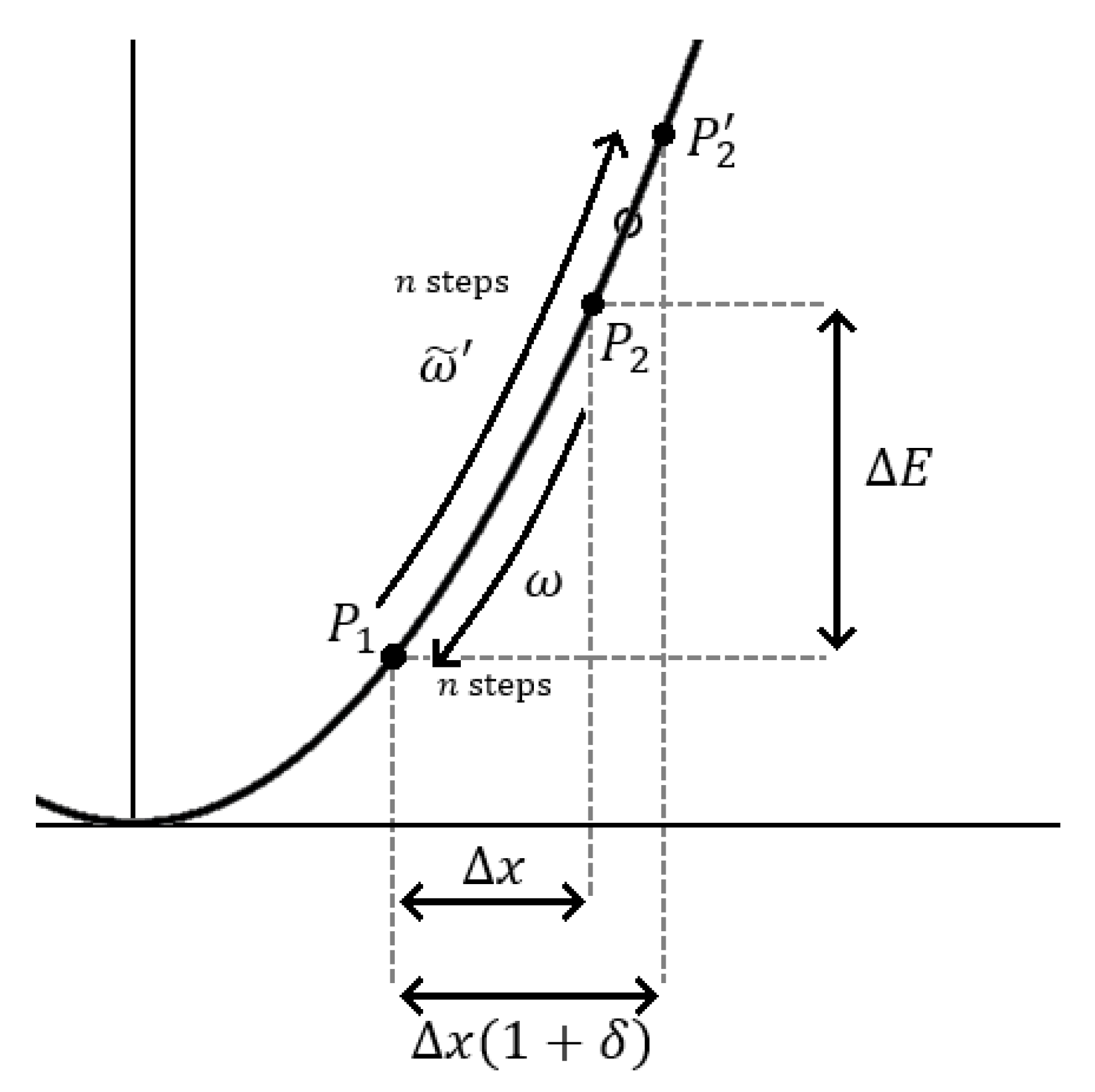
Consider Figure 2. We take two points, $P_1$ and $P_2$, on the parabolic potential of Figure 1a. The point $P_1$ is in the basin of attraction and the distance between the points is such that it takes more than one timestep to cover the trajectory. Say it would take n steps to go from $P_2$ to $P_1$ on a deterministic downslide. As discussed before, at equilibrium, the most likely upslide trajectory is the reverse of the deterministic downslide and also takes n steps. With the violation of microscopic reversibility that was discussed in the previous section, a mismatch arises. If the upslide speeds carry a factor $(1+\delta )$, then the n steps will bring the particle further up in the potential. Instead of the equilibrium distance $\Delta x$, a distance $\Delta x(1+\delta )$ would be covered and the point $P_2^{\prime }$ would be reached.

For the equilibrium situation, there is an elegant relation connecting any trajectory $\omega$ to its time-reverse $\tilde{\omega }$. Let $P\left(\omega \right)$ and $P\left(\tilde{\omega }\right)$ be the probabilities of the underlying sequences of steps for $\omega$ and $\tilde{\omega }$. We have [26]:

$$\frac{P\left(\tilde{\omega }\right)}{P\left(\omega \right)}=exp\left[-\frac{\Delta E}{k_{B}T}\right].$$

(13)

The right-hand side of the equation is recognized as the Boltzmann factor, i.e., the ratio of the population densities at $P_2$ and $P_1$. With Equation (13) we see that upslide and downslide ultimately occur equally often, i.e., we have microscopic reversibility.

With the small deviation from microscopic reversibility, we obtain the slightly mismatched situation: the starting point of the trajectory $\omega$ is a small distance away from the endpoint of ${\tilde{\omega }}^{\prime }$. What is a single point $P_2$ in the equilibrium state is a small segment at nonequilibrium. It is not unreasonable to hypothesize that the value of the probability density that, at equilibrium, corresponds to $P_2$ is achieved halfway between $P_2$ and $P_2^{\prime }$ at nonequilibrium. This point is indicated in Figure 2 with an open circle.

It is obvious that the augmentation of the upslides (cf. Figure 2) leads to a widening of the distribution. The standard deviation will increase, but it will not become infinite as with $\alpha$-stable distributions. In other words, we move towards the $\alpha <2$ situation without blowing up the standard deviation and other moments.

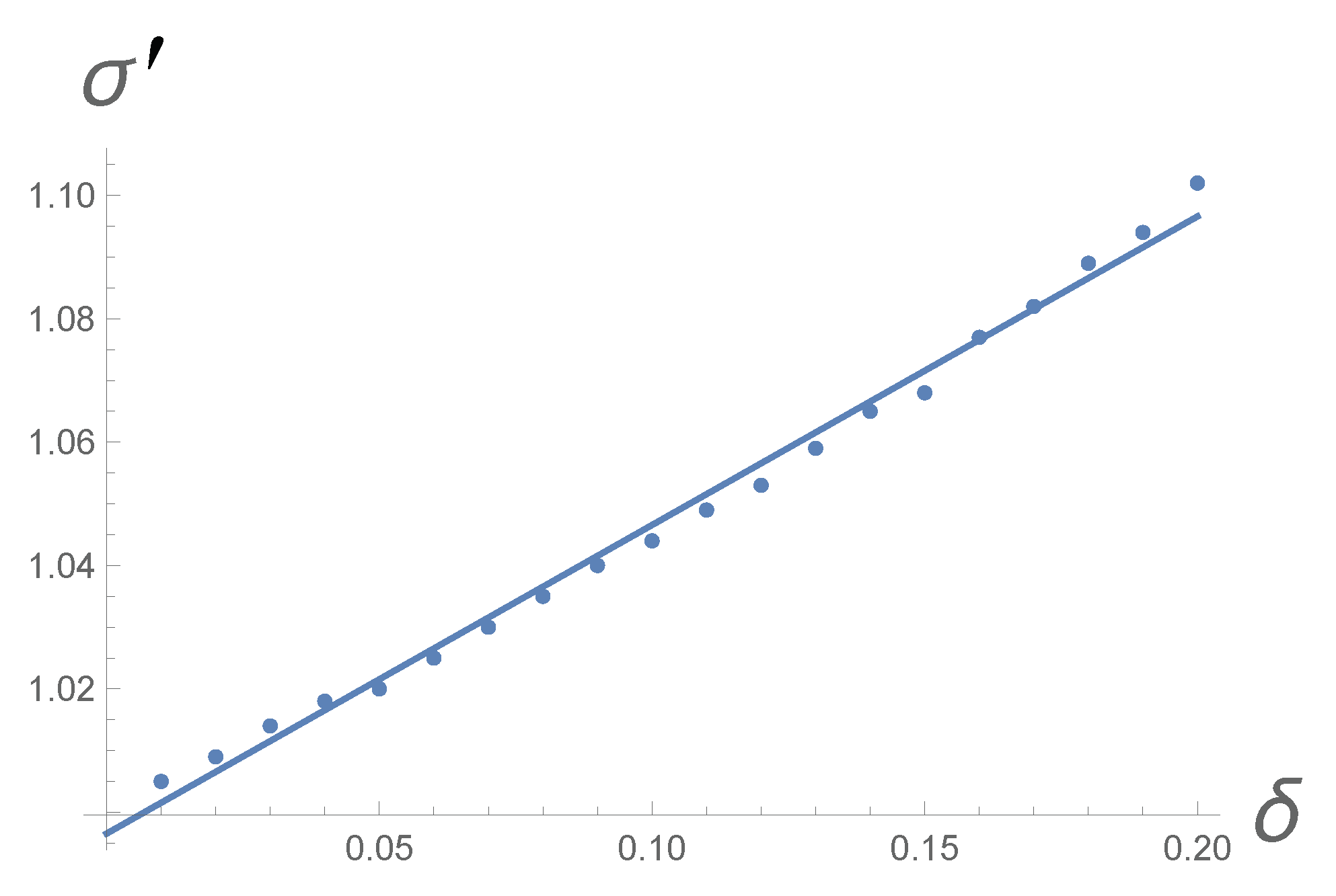
With Equation (3) and Gaussian noise, the stationary probability distribution for the position in a parabolic potential $V\left(x\right)=\frac{1}{2}A{x}^2$ is a zero-average Gaussian with a standard deviation of $\sigma =\sqrt{D/A}$ [1]. With the small violation of microscopic reversibility characterized by $\delta$, we expect that the probability density will still “look” very Gaussian, but it will have a standard deviation of ${\sigma }^{\prime }=\sigma (1+\delta /2)=\sigma (1+r)$ (cf. Figure 2). So the Gaussian will be stretched by a multiplicative factor $(1+r)$.

With $\sigma =\sqrt{D/A}$, we see that $\sqrt{D}$ gets a multiplicative factor $(1+r)$ upon going to nonequilibrium. This means that D gets, at first order, a factor $(1+2r)$, i.e., we retrieve Equation (12). With the FDR, $D=k_{B}T/\beta$, we see that Equation (11) follows concurrently.

The ideas put forward in the previous paragraphs can be readily checked through a Langevin simulation. The simulation is based on a Euler scheme using Equation (3). The coefficient of friction $\beta$ and the diffusion coefficient D are set equal to one, and we also pick $A=1$. The Euler scheme thus computes the increments and new positions using $\Delta x_i=-x_i\Delta t+{\theta }_{2,i}\sqrt{2\Delta t}$ and $x_{i+1}=x_i+\Delta x_i$, respectively, where ${\theta }_{2,i}$ is the i-th random number drawn from a Gaussian distribution with a zero average and a standard deviation of one. A breaking of time-reversal symmetry similar to the one brought about by Lévy jumps is applied by simply augmenting the climbing steps by a small fraction $\delta$. However, care must be taken here, as ${\sigma }^{\prime }=\sigma (1+\delta /2)$ is only obtained when some supplementary conditions are implemented.

Following the simple criterion for “climbing” formulated with Equation (6), the augmentation would also apply inside the basin of attraction. This would lead to the Gaussian distribution becoming bimodal, i.e., the distribution turning into one with with two maxima. Bimodal distributions have been observed more commonly in the context of Lévy noise in a potential well [27,28,29]. The bimodality is intriguing and worth further study, but here, we wish to stop it from occurring and maintain the Gaussian shape. We thus only apply the augmentation outside the basin of attraction, i.e., on the i-th step if $|x_i|>\widehat{x}$ and $\mathrm{sgn}(\Delta x_i)=\mathrm{sgn}\left(x_i\right)$. With this procedure, we “fatten” the tail of the position distribution without causing bimodality or bringing about an infinite standard deviation. Figure 3 shows how for $\widehat{x}=1.87$, i.e., almost two standard deviations from the center, we obtain the ${\sigma }^{\prime }=(1+\delta /2)$ that the theory predicts. For a Gaussian distribution with a unit standard deviation, the interval between $-1.87$ and $1.87$ contains 94% of the probability.

6. Discussion

Extension of the FDR to nonequilibrium is a challenge that has been taken up by many, and different approaches have been tried [10,30,31]. Our starting point is a Lévy-noise-subjected particle in a quadratic potential well. The quadratic potential well is generic in the sense that along any potential profile $V\left(x\right)$, the first term in the expansion around a minimum at $x=x_0$ is generally quadratic, i.e., $V\left(x\right)\approx V\left(x_0\right)+\frac{1}{2}{V}^{″}\left(x_0\right){(x-x_0)}^2$.

Lévy noise is characterized by the occurrence of frequent outliers. In everyday data-processing practice, however, the reasoning is often in the opposite direction: upon observation of frequent outliers it is inferred that the underlying noise must be Lévy. Subsequent theoretical analysis is then commonly greatly impaired by the divergent integrals that are associated with Lévy noise. In the face of these infinities, relating data and theory is no longer straightforward.

At that point, it makes sense to take a step back and realize that infinity is an abstraction. In the aforementioned setup of Kanazawa et al. [11], for instance, the liquid in an experimental realization has to be in a container, and it is obvious that no Lévy jump will ever be larger than the size of the container. Silva et al. [17] followed the spatial fluctuations of a cytoskeletal network and found fat tails in the ensuing distribution. Here likewise, the container size imposes a natural cutoff on the jump size. An infinite standard deviation is just as unrealistic as $\Delta t\to 0$ in our Equation (5).

With finite standard deviations, the Central Limit Theorem should apply again. This idea was what motivated Mantegna and Stanley as they took n different truncated $\alpha$-stable distributions [32]. They added the results of draws from these n distributions and found that convergence to a Gaussian occurs with increasing n, but it is very slow. Note that the position distribution that we arrive at in Section 5 is still Gaussian, but that it has just been artificially widened by the augmentation of the climbing steps.

In this article, we started with the observation that time-reversal symmetry is violated for a Lévy-noise-subjected particle in a harmonic well. The particle tends to “shoot up” and “slide down.” We quantified the “degree of violation” with a parameter r. For the Lévy-noise-subjected particle in a harmonic well, the standard deviation and the higher moments diverge. There is no temperature and no FDR. We devised a way to artificially implement a small amount of violation of the time-reversal symmetry. In this Discussion section, we explained why it is sensible and realistic to keep all the involved moments finite. Our scheme does not give rise to divergent integrals and leads to simple expressions for a corrected FDR. The correction only involves the parameter r.

A possible experimental verification of Equations (10) and (12) would entail a setup with an energy input; an energy input leading to a bath with particles whose motion violates time-reversal symmetry. Through following that motion with a probe, the r could possibly be established. The power dissipation or the diffusion coefficient could next be established independently.