On Strengthened Extragradient Methods Non-Convex Combination with Adaptive Step Sizes Rule for Equilibrium Problems

Abstract

Symmetries play a vital role in the study of physical phenomena in diverse areas such as dynamic systems, optimization, physics, scientific computing, engineering, mathematical biology, chemistry, and medicine, to mention a few. These phenomena specialize mostly in solving equilibria-like problems in abstract spaces. Motivated by these facts, this research provides two innovative modifying extragradient strategies for solving pseudomonotone equilibria problems in real Hilbert space with the Lipschitz-like bifunction constraint. Such strategies make use of multiple step-size concepts that are modified after each iteration and are reliant on prior iterations. The excellence of these strategies comes from the fact that they were developed with no prior knowledge of Lipschitz-type parameters or any line search strategy. Mild assumptions are required to prove strong convergence theorems for proposed strategies. Various numerical tests have been reported to demonstrate the numerical behavior of the techniques and then contrast them with others.

1. Introduction

Consider that $\Sigma$ is a nonempty, convex, and closed subset of a real Hilbert space $\Pi .$ The inner product and norm are indicated with $\langle .,.\rangle$ and $\parallel .\parallel ,$ respectively. Furthermore, $\mathbb{R}$ and $\mathbb{N}$ symbolize the set of real numbers and the set of natural numbers, respectively. Assume that $\mathcal{R}:\Pi \times \Pi \to \mathbb{R}$ is indeed a bifunction with the equilibrium problem solution set $EP(\mathcal{R},\Sigma ).$ Let

$$s^{*}=P_{EP(\mathcal{R},\Sigma )},$$

whereas $\theta$ represents a zero element in $\Pi .$ In this case, $\Sigma$ characterizes the subset of a Hilbert space $\Pi$ and $\mathcal{R}$ as follows: $\mathcal{R}:\Pi \times \Pi \to \mathbb{R}$ is a bifunction through $\mathcal{R}(r_1,r_1)=0,$ for all $r_1\in \Sigma .$ The equilibrium problem [1,2] for $\mathcal{R}$ on $\Sigma$ is to:

$$\mathrm{Find}{s}^{*}\in \Sigma \mathrm{such}\mathrm{that}\mathcal{R}(s^{*},r_1)\ge 0,\forall r_1\in \Sigma .$$

(1)

The above-mentioned framework is an appropriate mathematical framework that incorporates a variety of problems, including vector and scalar minimization problems, saddle point problems, variational inequality problems, complementarity problems, Nash equilibrium problems in non-cooperative games, and inverse optimization problems [1,3,4]. This issue is primarily connected to Ky Fan inequity on the grounds of his prior contributions to the field [2]. It is also important to consider an approximate solution if the problem does not have an exact solution or is difficult to calculate. Several methodologies have been proposed and tested to tackle various types of equilibrium problems (1). Many successful algorithmic techniques, as well as theoretical characteristics, have already been proposed to solve the (1) issue in both finite- and infinite-dimensional spaces.

The regularization technique is the most significant method for dealing with many ill-posed problems in various subfields of applied and pure mathematics. The regularization approach is distinguished by the use of monotone equilibrium problems to convert the original problem into a strongly monotone equilibrium subproblem. As a result, each computationally productive subproblem is strongly monotone and has a unique solution. The discovered subproblem, for example, may be more successfully resolved than the initial problem, and the regularization solutions may lead to some solution to the basic problem once the regularization variables look to have an adequate limit. The two most prevalent regularization methods are the proximal point and Tikhonov’s regularized approaches. These approaches were recently extended to equilibrium problems [5,6,7,8,9,10,11,12,13]. A few techniques to address non-monotone equilibrium problems can be found in [14,15,16,17,18,19,20,21,22,23,24,25,26].

The proximal method [27] is indeed an innovative approach for determining equilibrium problems that are founded on minimization problems. Along with Korpelevich’s contribution [28] technique to addressing the saddle point problem, this procedure has also been known as the two-step extragradient method in [29]. Tran et al. [29] constructed an iterative sequence of $\left\{s_k\right\}$ in the following manner:

$$\left\{\begin{array}{c}{s}_1\in \Sigma ,\hfill \\ m_k=\underset{v\in \Sigma }{argmin}\{\lambda \mathcal{R}(s_k,v)+\frac{1}{2}\parallel s_k-v{\parallel }^2\},\hfill \\ s_{k+1}=\underset{v\in \Sigma }{argmin}\{\lambda \mathcal{R}(m_k,v)+\frac{1}{2}\parallel s_k-v{\parallel }^2\},\hfill \end{array}\right.$$

where $0<\lambda <min\left\{\frac{1}{2c_1},\frac{1}{2c_2}\right\}.$ The iterative sequence created by the aforementioned approach exhibits weak convergence, and prior knowledge of Lipschitz-type variables is necessary in order to use it. Lipschitz-type parameters are frequently unknown or difficult to calculate. To address this issue, Hieu et al. [30] introduced the following adaptation of the approach in [31] for equilibrium: Let ${\left[t\right]}_{+}=max\{t,0\}$ and select $s_1\in \Sigma ,$ $\mu \in (0,1)$ with ${\lambda }_0>0,$ such that

$$\left\{\begin{array}{c}{m}_k=\underset{v\in \Sigma }{argmin}\{{\lambda }_k\mathcal{R}(s_k,v)+\frac{1}{2}\parallel s_k-v{\parallel }^2\},\hfill \\ s_{k+1}=\underset{v\in \Sigma }{argmin}\{{\lambda }_k\mathcal{R}(m_k,v)+\frac{1}{2}\parallel s_k-v{\parallel }^2\},\hfill \end{array}\right.$$

along with

$${\lambda }_{k+1}=min\left\{{\lambda }_k,\frac{\mu (\parallel s_k-m_k{\parallel }^2+\parallel s_{k+1}-m_k{\parallel }^2)}{2{[\mathcal{R}(s_k,s_{k+1})-\mathcal{R}(s_k,m_k)-\mathcal{R}(m_k,s_{k+1})]}_{+}}\right\}.$$

To solve a pseudomonotone equilibrium problem, the authors have suggested a non-convex combination iterative technique in [32]. The availability of a strong convergence iterative sequence without the need for hybrid projection or viscosity techniques is the main contribution. The details of the algorithm are as follows: Choose $0<{\lambda }_k<min\left\{\frac{1}{2c_1},\frac{1}{2c_2}\right\},$ ${\delta }_k\subset [\delta ,1)$ with $\delta >0$ and ${\varphi }_k$ such that

$$\underset{k\to +\infty }{lim}{\varphi }_k=0\mathrm{and}\sum _{k=1}^{+\infty }{\varphi }_k=+\infty .$$

$$\left\{\begin{array}{c}{m}_k=\underset{v\in \Sigma }{argmin}\{{\lambda }_k\mathcal{R}(s_k,v)+\frac{1}{2}\parallel s_k-v{\parallel }^2\},\hfill \\ r_k=\underset{v\in \Sigma }{argmin}\{{\lambda }_k\mathcal{R}(m_k,v)+\frac{1}{2}\parallel s_k-v{\parallel }^2\},\hfill \end{array}\right.$$

and

$$s_{k+1}=P_{\Sigma }\left[{\varphi }_k{s}_k+(1-{\varphi }_k)r_k-{\varphi }_k{\delta }_k{s}_k\right].$$

The main objective of this study is to focus on using well-known projection algorithms that are, in general, easier to apply due to their efficient and easy mathematical computation. We design and adapt an explicit subgradient extragradient method to solve the problem of pseudomonotone equilibrium and other specific classes of variational inequality problems and fixed-point problems, inspired by the works of [30,33]. Our techniques are a variation on the approaches described in [32]. Strong convergence results matching the sequence of the two methods are achieved under specific, moderate circumstances. Some applications of variational inequality and fixed-point problems are given. Consequently, experimental investigations have shown that the proposed strategy is more successful than the current one [32].

The rest of the article is organized as follows: Section 2 includes basic definitions and lemmas. Section 3 proposes new methods and their convergence analysis theorems. Section 4 contains several applications of our findings to variational inequality and fixed-point problems. Section 5 contains numerical tests to demonstrate the computational effectiveness of our proposed methods.

2. Preliminaries

Suppose that a convex function $\Im :\Sigma \to \mathbb{R}$ and subdifferential of ℑ at $r_1\in \Sigma$ is expressed as follows:

$$\partial \Im \left(r_1\right)=\{r_3\in \Pi :\Im \left(r_2\right)-\Im \left(r_1\right)\ge \langle r_3,r_2-r_1\rangle ,\forall r_2\in \Sigma \}.$$

A normal cone of Σ at $r_1\in \Sigma$ is expressed as follows:

$$N_{\Sigma }\left(r_1\right)=\{r_3\in \Pi :\langle r_3,r_2-r_1\rangle \le 0,\forall r_2\in \Sigma \}.$$

Lemma 1.

([34]) Suppose that a convex function $\Im :\Sigma \to \mathbb{R}$ is subdifferentiable and lower semicontinuous upon $\Sigma .$ Then $r_1\in \Sigma$ is a minimizer of a function ℑ if and only if

$$0\in \partial \Im \left(r_1\right)+N_{\Sigma }\left(r_1\right),$$

where $\partial \Im \left(r_1\right)$ and $N_{\Sigma }\left(r_1\right)$ denotes the subdifferential of ℑ at $r_1\in \Sigma$ and the normal cone of Σ at $r_1,$ respectively.

Definition 1.

([35]) A metric projection $P_{\Sigma }\left(r_1\right)$ for $r_1\in \Pi$ onto a convex and closed subset Σ of Π is stated as follows:

$$P_{\Sigma }\left(r_1\right)=\underset{}{argmin}\{\parallel r_2-r_1\parallel :r_2\in \Sigma \}.$$

Lemma 2.

([36]) Consider that a metric projection $P_{\Sigma }:\Pi \to \Sigma .$ Then

(i)

For some $r_2\in \Sigma$ and $r_1\in \Pi$ in order that

$$\parallel r_1-P_{\Sigma }\left(r_1\right)\parallel \le \parallel r_1-r_2{\parallel }^2.$$

(ii)

$r_3=P_{\Sigma }\left(r_1\right)$ if and only if

$$\langle r_1-r_3,r_2-r_3\rangle \le 0,\forall r_2\in \Sigma .$$

Lemma 3.

([37]) For some $r_1,r_2\in \Pi$ and $\chi \in \mathbb{R}.$ Then

(i)

$$\parallel \chi r_1+(1-\chi )r_2{\parallel }^2=\chi \parallel r_1{\parallel }^2+(1-\chi )\parallel r_2{\parallel }^2-\chi (1-\chi ){\parallel r_1-r_2\parallel }^2;$$

(ii)

$$\parallel r_1+r_2{\parallel }^2\le {\parallel r_1\parallel }^2+2\langle r_2,r_1+r_2\rangle .$$

Lemma 4.

([38]) Consider a sequence of non-negative real numbers $\left\{{\chi }_k\right\}$ such that

$${\chi }_{k+1}\le (1-{\tau }_k){\chi }_k+{\tau }_k{\delta }_k,\forall k\in \mathbb{N},$$

while $\left\{{\tau }_k\right\}\subset (0,1)$ and $\left\{{\delta }_k\right\}\subset \mathbb{R}$ conforming to the following parameters:

$$\underset{k\to +\infty }{lim}{\tau }_k=0,\sum _{k=1}^{+\infty }{\tau }_k=+\infty ,and\underset{k\to +\infty }{lim\; sup}{\delta }_k\le 0.$$

Thus, ${lim}_{k\to +\infty }{\chi }_k=0.$

Lemma 5.

([39]) Assume that $\left\{{\chi }_k\right\}$ is a sequence of real numbers namely that there exists a subsequence $\left\{k_i\right\}$ of $\left\{k\right\}$ such that

$${\chi }_{k_i}<{\chi }_{k_{i+1}},foralli\in \mathbb{N}.$$

Then, there would be a nondecreasing sequence $\left\{e_k\right\}\subset \mathbb{N}$, namely that $e_k\to +\infty$ as $k\to +\infty ,$ and the following criteria are fulfilled by all (sufficiently big) integers $k\in \mathbb{N}:$

$${\chi }_{e_k}\le {\chi }_{m_{k+1}}\mathrm{and}{\chi }_k\le {\chi }_{m_{k+1}}.$$

In fact, $e_k=max\{j\le k:{\chi }_j\le {\chi }_{j+1}\}.$

Now, we consider the following bifunction monotonicity notions (for more information, see [1,40]). A bifunction $\mathcal{R}:\Pi \times \Pi \to \mathbb{R}$ on $\Sigma$ for $\xi >0$ such that

(1) strongly monotone if

$$\mathcal{R}(r_1,r_2)+\mathcal{R}(r_2,r_1)\le -\xi {\parallel r_1-r_2\parallel }^2,\forall r_1,r_2\in \Sigma ;$$

(2) monotone if

$$\mathcal{R}(r_1,r_2)+\mathcal{R}(r_2,r_1)\le 0,\forall r_1,r_2\in \Sigma ;$$

(3) strongly pseudomonotone if

$$\mathcal{R}(r_1,r_2)\ge 0⟹\mathcal{R}(r_2,r_1)\le -\xi {\parallel r_1-r_2\parallel }^2,\forall r_1,r_2\in \Sigma ;$$

(4) pseudomonotone if

$$\mathcal{R}(r_1,r_2)\ge 0⟹\mathcal{R}(r_2,r_1)\le 0,\forall r_1,r_2\in \Sigma .$$

Suppose that $\mathcal{R}:\Pi \times \Pi \to \mathbb{R}$ meets the Lipschitz-type condition [41] over $\Sigma$ if $c_1,c_2>0,$ such that

$$\mathcal{R}(r_1,r_3)\le \mathcal{R}(r_1,r_2)+\mathcal{R}(r_2,r_3)+c_1\parallel r_1-r_2{\parallel }^2+c_2{\parallel r_2-r_3\parallel }^2,\forall r_1,r_2,r_3\in \Sigma .$$

We shall presume that the requirements listed below have been satisfied. A bifunction $\mathcal{R}$ meets the following criteria:

($\mathcal{R}$1)

$\mathcal{R}(r_2,r_2)=0$ for all $r_2\in \Sigma$ and $\mathcal{R}$ is pseudomonotone on feasible set $\Sigma ;$

($\mathcal{R}$2)

$\mathcal{R}$ meet the Lipschitz-type condition on $\Pi$ with constants $c_1$ and $c_2;$

($\mathcal{R}$3)

$\mathcal{R}(r_1,r_2)$ is jointly weakly continuous on $\Pi \times \Pi$;

($\mathcal{R}$4)

$\mathcal{R}(r_1,.)$ need to be convex and subdifferentiable over $\Pi$ for each $r_1\in \Pi .$

3. Main Results

We add a method and have strong convergence results for that method. The following is a detailed algorithm:

The following lemma can be used to demonstrate that the step-size sequence ${\lambda }_k$ generated by the previous formula decreases monotonically and is bounded, as required for iterative sequence convergence.

Lemma 6.

A sequence $\left\{{\lambda }_k\right\}$ is decreasing monotonically with lower bound $min\left\{\frac{\mu }{2max\{c_1,c_2\}},{\lambda }_0\right\}$ and converge to $\lambda >0.$

Proof. 

It is straightforward that $\left\{{\lambda }_k\right\}$ decreases monotonically. Let $\mathcal{R}(s_k,r_k)-\mathcal{R}(s_k,m_k)-\mathcal{R}(m_k,r_k)>0$, such that

$$\begin{array}{cc}\hfill & \frac{\mu (\parallel s_k-m_k{\parallel }^2+\parallel r_k-m_k{\parallel }^2)}{2[\mathcal{R}(s_k,r_k)-\mathcal{R}(s_k,m_k)-\mathcal{R}(m_k,r_k)]}\hfill \\ \hfill & \ge \frac{\mu (\parallel s_k-m_k{\parallel }^2+\parallel r_k-m_k{\parallel }^2)}{2[c_1\parallel s_k-m_k{\parallel }^2+c_2\parallel r_k-m_k{\parallel }^2]}\ge \frac{\mu }{2max\{c_1,c_2\}}.\hfill \end{array}$$

Thus, sequence $\left\{{\lambda }_k\right\}$ has the lower bound $min\left\{\frac{\mu }{2max\{c_1,c_2\}},{\lambda }_0\right\}.$ Thus, there exists a real number $\lambda >0,$ to ensure that ${lim}_{k\to +\infty }{\lambda }_k=\lambda .$    □

The following lemma can be used to verify the boundedness of an iterative sequence.

Lemma 7.

Let $\mathcal{R}:\Pi \times \Pi \to \mathbb{R}$ be a bifunction that satisfies the conditions($\mathcal{R}$1)–($\mathcal{R}$4). For any $s^{*}\in EP(\mathcal{R},\Sigma )\ne \varnothing ,$ we have

$$\parallel r_k-s^{*}{\parallel }^2\le \parallel s_k-s^{*}{\parallel }^2-\left(1-\frac{\mu {\lambda }_k}{{\lambda }_{k+1}}\right)\parallel s_k-m_k{\parallel }^2-\left(1-\frac{\mu {\lambda }_k}{{\lambda }_{k+1}}\right){\parallel r_k-m_k\parallel }^2.$$

Proof. 

By the value $r_k$ and Lemma 1, we obtain

$${\lambda }_k\mathcal{R}(m_k,y)-{\lambda }_k\mathcal{R}(m_k,r_k)\ge \langle s_k-r_k,y-r_k\rangle ,\forall y\in {\Pi }_k.$$

(2)

From definition of ${\Pi }_k,$ we have

$${\lambda }_k\mathcal{R}(s_k,r_k)-{\lambda }_k\mathcal{R}(s_k,m_k)\ge \langle s_k-m_k,r_k-m_k\rangle .$$

(3)

Using the value of ${\lambda }_{k+1},$ we can write

$$\mathcal{R}(s_k,r_k)-\mathcal{R}(s_k,m_k)-\mathcal{R}(m_k,r_k)\le \frac{\mu (\parallel s_k-m_k{\parallel }^2+\parallel r_k-m_k{\parallel }^2)}{2{\lambda }_{k+1}}.$$

(4)

Expressions (2)–(4) imply that (see Lemma 3.3 in [42]):

$$\parallel r_k-s^{*}{\parallel }^2\le \parallel s_k-s^{*}{\parallel }^2-\left(1-\frac{\mu {\lambda }_k}{{\lambda }_{k+1}}\right)\parallel s_k-m_k{\parallel }^2-\left(1-\frac{\mu {\lambda }_k}{{\lambda }_{k+1}}\right){\parallel r_k-m_k\parallel }^2.$$

   □

The strong convergence analysis for Algorithm 1 is presented in the following theorem. The details of the convergence theorems are given below.

Algorithm 1 Self-Adaptive Explicit Extragradient Method with Non-Convex Combination

Step 0: Let $s_1\in \Pi ,$${\lambda }_0>0$, $\mu \in (0,1),$${\delta }_k\subset [\delta ,1)$ through $\delta >0$ and ${\varphi }_k\subset (0,1)$ such that $$\underset{k\to +\infty }{lim}{\varphi }_k=0\mathrm{and}\sum _{k=1}^{+\infty }{\varphi }_k=+\infty .$$ Step 1: Compute $$m_k=\underset{v\in \Sigma }{argmin}\{{\lambda }_k\mathcal{R}(s_k,v)+\frac{1}{2}\parallel s_k-v{\parallel }^2\}.$$ In the case that $m_k=s_k,$ stop and $s_k\in EP(\mathcal{R},\Sigma )$. Otherwise, go to the next step. Step 2: First, choose ${\omega }_k\in \partial \mathcal{R}(s_k,m_k)$ satisfying $s_k-{\lambda }_k{\omega }_k-m_k\in N_{\mathcal{K}}\left(m_k\right)$ and generate a half-space $${\Pi }_k=\{z\in \Pi :\langle s_k-{\lambda }_k{\omega }_k-m_k,z-m_k\rangle \le 0\}.$$ Solve $r_k=\underset{v\in {\Pi }_k}{argmin}\{{\lambda }_k\mathcal{R}(m_k,v)+\frac{1}{2}\parallel s_k-v{\parallel }^2\}.$ Step 3: Compute $$s_{k+1}=P_{\Sigma }\left[{\varphi }_k{s}_k+(1-{\varphi }_k)r_k-{\varphi }_k{\delta }_k{s}_k\right].$$ Step 4: Revise the step size as follows and continue: $${\lambda }_{k+1}=\left\{\begin{array}{l}min\left\{{\lambda }_k,\frac{\mu (\parallel s_k-m_k{\parallel }^2+\parallel r_k-m_k{\parallel }^2)}{2[\mathcal{R}(s_k,r_k)-\mathcal{R}(s_k,m_k)-\mathcal{R}(m_k,r_k)]}\right\}\hfill \\ \mathrm{if}\mathcal{R}(s_k,r_k)-\mathcal{R}(s_k,m_k)-\mathcal{R}(m_k,r_k)>0\\ {\lambda }_k\mathrm{otherwise}.\end{array}\right.$$ Set $k:=k+1$ and move back to Step 1.

Theorem 1.

Let a sequence $\left\{s_k\right\}$ be generated by Algorithm 1. Then, sequence $\left\{s_k\right\}$ converges strongly to $s^{*}\in EP(\mathcal{R},\Sigma ).$

Proof. 

Given that ${\lambda }_k\to \lambda ,$ then $ϵ\in (0,1-\mu ),$ is a number such that

$$\underset{k\to +\infty }{lim}\left(1-\frac{\mu {\lambda }_k}{{\lambda }_{k+1}}\right)=1-\mu >ϵ>0.$$

As a result, there exists a finite number $k_1\in \mathbb{N}$ such that

$$\left(1-\frac{\mu {\lambda }_k}{{\lambda }_{k+1}}\right)>ϵ>0,\forall k\ge k_1.$$

(5)

Using Lemma 7, we have

$$\parallel r_k-s^{*}{\parallel }^2\le {\parallel s_k-s^{*}\parallel }^2,\forall k\ge k_1.$$

(6)

We derive using Lemma 3 (i) for any $k\ge k_1,$ such that

$$\begin{array}{cc}\hfill \parallel s_{k+1}-s^{*}{\parallel }^2 & =\parallel P_{\Sigma }\left[{\varphi }_k(1-{\delta }_k)s_k+(1-{\varphi }_k)r_k\right]-P_{\Sigma }\left(s^{*}\right){\parallel }^2\hfill \\ \hfill & \le \parallel {\varphi }_k(1-{\delta }_k)s_k+(1-{\varphi }_k)r_k-s^{*}{\parallel }^2\hfill \\ \hfill & =\parallel {\varphi }_k\left[(1-{\delta }_k)s_k-s^{*}\right]+(1-{\varphi }_k)(r_k-s^{*}){\parallel }^2\hfill \\ \hfill & \le {\varphi }_k\parallel (1-{\delta }_k)s_k-s^{*}{\parallel }^2+(1-{\varphi }_k){\parallel r_k-s^{*}\parallel }^2\hfill \\ \hfill & \le {\varphi }_k\left[\parallel (1-{\delta }_k)(s_k-s^{*})+{\delta }_k{s}^{*}{\parallel }^2\right]+(1-{\varphi }_k){\parallel s_k-s^{*}\parallel }^2\hfill \\ \hfill & -(1-{\varphi }_k)\left[\left(1-\frac{\mu {\lambda }_k}{{\lambda }_{k+1}}\right)\parallel s_k-m_k{\parallel }^2+\left(1-\frac{\mu {\lambda }_k}{{\lambda }_{k+1}}\right){\parallel r_k-m_k\parallel }^2\right]\hfill \\ \hfill & \le {\varphi }_k\left[(1-{\delta }_k)\parallel s_k-s^{*}{\parallel }^2+{\delta }_k{\parallel s^{*}\parallel }^2\right]+(1-{\varphi }_k){\parallel s_k-s^{*}\parallel }^2\hfill \\ \hfill & -(1-{\varphi }_k)\left[ϵ\parallel s_k-m_k{\parallel }^2+ϵ{\parallel r_k-m_k\parallel }^2\right]\hfill \\ \hfill & =(1-{\varphi }_k{\delta }_k)\parallel s_k-s^{*}{\parallel }^2+{\varphi }_k{\delta }_k{\parallel s^{*}\parallel }^2\hfill \end{array}$$

$$\begin{array}{cc}\hfill & -ϵ(1-{\varphi }_k)\left[\parallel s_k-m_k{\parallel }^2+{\parallel r_k-m_k\parallel }^2\right]\hfill \\ \hfill & \le max\{\parallel s_k-s^{*}{\parallel }^2,\parallel s^{*}{\parallel }^2\}\hfill \end{array}$$

(7)

$$\begin{array}{cc}\hfill & \le max\{\parallel s_{k_1}-s^{*}{\parallel }^2,\parallel s^{*}{\parallel }^2\}.\hfill \end{array}$$

(8)

It is deduced that sequence $\left\{s_k\right\}$ is a bounded sequence. Let $q_k={\varphi }_k{s}_k+(1-{\varphi }_k)r_k,$ for any $k\in \mathbb{N}.$ By Lemma 3 (i), we have

$$\begin{array}{cc}\hfill \parallel q_k-s^{*}{\parallel }^2& = \parallel {\varphi }_k{s}_k+(1-{\varphi }_k)r_k-s^{*}{\parallel }^2\le {\parallel s_k-s^{*}\parallel }^2,\forall k\ge k_1.\hfill \end{array}$$

(9)

Notice that there is

$$\begin{array}{cc}\hfill s_{k+1}& =P_{\Sigma }(q_k-{\varphi }_k{\delta }_k{s}_k)=P_{\Sigma }\left[(1-{\varphi }_k{\delta }_k)q_k+{\varphi }_k{\delta }_k(1-{\varphi }_k)(r_k-s_k)\right].\hfill \end{array}$$

(10)

By Lemma 3 (ii) and (9), (10) implies that (see Equation (3.6) [32])

$$\begin{array}{cc}\hfill & \parallel s_{k+1}-s^{*}{\parallel }^2\hfill \\ \hfill & =\parallel P_{\Sigma }\left[(1-{\varphi }_k{\delta }_k)q_k+{\varphi }_k{\delta }_k(1-{\varphi }_k)(r_k-s_k)\right]-P_{\Sigma }\left(s^{*}\right){\parallel }^2\hfill \\ \hfill & \le (1-{\varphi }_k{\delta }_k){\parallel s_k-s^{*}\parallel }^2+2{\varphi }_k{\delta }_k(1-{\varphi }_k)\hfill \\ \hfill & 〈r_k-s_k,(1-{\varphi }_k{\delta }_k)q_k+{\varphi }_k{\delta }_k(1-{\varphi }_k)(r_k-s_k)-s^{*}〉\hfill \\ \hfill & +2{\varphi }_k{\delta }_k(1-{\varphi }_k)〈-s^{*},r_k-s_k〉+2{\varphi }_k{\delta }_k〈-s^{*},s_k-s^{*}〉+2{\varphi }_k^2{\delta }_k^2〈s^{*},s_k〉.\hfill \end{array}$$

(11)

The remains of the proof can be split into two parts:

Case 1: Let $k_2\in \mathbb{N}$$(k_2\ge k_1)$ such that

$$\parallel s_{k+1}-s^{*}\parallel \le \parallel s_k-s^{*}\parallel ,\forall k\ge k_2.$$

Thus, ${lim}_{k\to +\infty }\parallel s_k-s^{*}\parallel$, exists and let ${lim}_{k\to +\infty }\parallel s_k-s^{*}\parallel =l.$ By relationship (7), we have

$$\begin{array}{cc}\hfill ϵ\left[\parallel s_k-m_k{\parallel }^2+{\parallel r_k-m_k\parallel }^2\right]& \le \parallel s_k-s^{*}{\parallel }^2-\parallel s_{k+1}-s^{*}{\parallel }^2+{\varphi }_k{\delta }_k{\parallel s^{*}\parallel }^2\hfill \\ \hfill & +ϵ{\varphi }_k\left[\parallel s_k-m_k{\parallel }^2+{\parallel r_k-m_k\parallel }^2\right],\forall k\ge k_2.\hfill \end{array}$$

(12)

The existence of ${lim}_{k\to +\infty }\parallel s_k-s^{*}\parallel =l,$ provides that

$$\underset{k\to +\infty }{lim}\parallel s_k-m_k\parallel =\underset{k\to +\infty }{lim}\parallel r_k-m_k\parallel =0,$$

(13)

and accordingly

$$\underset{k\to +\infty }{lim}\parallel s_k-r_k\parallel \le \underset{k\to +\infty }{lim}\parallel s_k-m_k\parallel +\underset{k\to +\infty }{lim}\parallel m_k-r_k\parallel =0.$$

(14)

Thus, the sequence $\left\{s_k\right\}$ is a bounded sequence. Hence, we may select a subsequence $\left\{s_{k_j}\right\}$ of $\left\{s_k\right\}$ such that $\left\{s_{k_j}\right\}$ converges weakly to a certain $s\in \Sigma$ such that

$$\underset{k\to +\infty }{lim\; sup}\langle -s^{*},s_k-s^{*}\rangle =\underset{j\to +\infty }{lim\; sup}\langle -s^{*},s_{k_j}-s^{*}\rangle =\langle -s^{*},s-s^{*}\rangle .$$

(15)

From (13) the subsequence $\left\{m_{k_j}\right\}$ also converges weakly to s as $j\to +\infty .$ Due to the expression (3), we obtain

$${\lambda }_{k_j}\mathcal{R}(s_{k_j},y)-{\lambda }_{k_j}\mathcal{R}(s_{k_j},m_{k_j})\ge \langle s_{k_j}-m_{k_j},y-m_{k_j}\rangle ,\forall y\in \Sigma .$$

(16)

Allowing $j\to +\infty$ entails that

$$\mathcal{R}(s,y)\ge 0,\forall y\in \Sigma .$$

(17)

As a result, $s\in EP(\mathcal{R},\Sigma ).$ Eventually, using (15) and Lemma 2 (ii), we derive

$$\begin{array}{cc}\hfill \underset{k\to +\infty }{lim\; sup}\langle -s^{*},s_k-s^{*}\rangle & =\underset{j\to +\infty }{lim\; sup}\langle -s^{*},s_{k_j}-s^{*}\rangle \hfill \\ \hfill & =\langle -s^{*},s-s^{*}\rangle .\hfill \\ \hfill & =\langle \theta -P_{EP(\mathcal{R},\Sigma )},s-P_{EP(\mathcal{R},\Sigma )}\rangle .\hfill \\ \hfill & \le 0.\hfill \end{array}$$

(18)

We have the desired results from of the assertion on ${\varphi }_k,$${\delta }_k$, (11), (13), (14), (18) and Lemma 4.

Case 2: Assume that there exists a subsequence $\left\{k_i\right\}$ of $\left\{k\right\}$ such that

$$\parallel s_{k_i}-s^{*}\parallel \le \parallel s_{k_{i+1}}-s^{*}\parallel ,\forall i\in \mathbb{N}.$$

Consequently, according to Lemma 5, there is indeed a sequence $\left\{n_j\right\}\subset \mathbb{N}$ such that $n_j\to +\infty ,$ we have

$$\parallel s_{n_j}-s^{*}\parallel \le \parallel s_{m_{j+1}}-s^{*}\parallel \mathrm{and}\parallel s_j-s^{*}\parallel \le \parallel s_{m_{j+1}}-s^{*}\parallel ,\mathrm{for}\mathrm{all}j\in \mathbb{N}.$$

(19)

By the expression (7), we have

$$\begin{array}{cc}\hfill ϵ\left[\parallel s_{n_j}-m_{n_j}{\parallel }^2+{\parallel r_{n_j}-m_{n_j}\parallel }^2\right]& \le \parallel s_{n_j}-s^{*}{\parallel }^2-\parallel s_{n_j+1}-s^{*}{\parallel }^2+{\varphi }_{n_j}{\delta }_{n_j}{\parallel s^{*}\parallel }^2\hfill \\ \hfill & +ϵ{\varphi }_{n_j}\left[\parallel s_{n_j}-m_{n_j}{\parallel }^2+{\parallel r_{n_j}-m_{n_j}\parallel }^2\right],\forall n_j\ge k_1.\hfill \end{array}$$

(20)

The above expressions imply that

$$\underset{j\to +\infty }{lim}\parallel s_{n_j}-m_{n_j}\parallel =\underset{j\to +\infty }{lim}\parallel r_{n_j}-m_{n_j}\parallel =0,$$

(21)

thus

$$\underset{j\to +\infty }{lim}\parallel s_{n_j}-r_{n_j}\parallel \le \underset{j\to +\infty }{lim}\parallel s_{n_j}-m_{n_j}\parallel +\underset{j\to +\infty }{lim}\parallel m_{n_j}-r_{n_j}\parallel =0.$$

(22)

By statements identical to those in expression (18), we have

$$\underset{j\to +\infty }{lim\; sup}\langle -s^{*},s_{n_j}-s^{*}\rangle \le 0.$$

(23)

From expression (11), we obtain

$$\begin{array}{cc}\hfill & \parallel s_{n_j+1}-s^{*}{\parallel }^2\hfill \\ \hfill & \le (1-{\varphi }_{n_j}{\delta }_{n_j}){\parallel s_{n_j}-s^{*}\parallel }^2+2{\varphi }_{n_j}{\delta }_{n_j}(1-{\varphi }_{n_j})\hfill \\ \hfill & 〈r_{n_j}-s_{n_j},(1-{\varphi }_{n_j}{\delta }_{n_j})q_{n_j}+{\varphi }_{n_j}{\delta }_{n_j}(1-{\varphi }_{n_j})(r_{n_j}-s_{n_j})-s^{*}〉\hfill \\ \hfill & +2{\varphi }_{n_j}{\delta }_{n_j}(1-{\varphi }_{n_j})〈-s^{*},r_{n_j}-s_{n_j}〉+2{\varphi }_{n_j}{\delta }_{n_j}〈-s^{*},s_{n_j}-s^{*}〉+2{\varphi }_{n_j}^2{\delta }_{n_j}^2〈s^{*},s_{n_j}〉.\hfill \end{array}$$

(24)

It is given that $\parallel s_{n_j}-s^{*}\parallel \le \parallel s_{m_{j+1}}-s^{*}\parallel ,$ implies that

$$\begin{array}{cc}\hfill & \parallel s_{n_j+1}-s^{*}{\parallel }^2\hfill \\ \hfill & \le (1-{\varphi }_{n_j}{\delta }_{n_j}){\parallel s_{m_{j+1}}-s^{*}\parallel }^2+2{\varphi }_{n_j}{\delta }_{n_j}(1-{\varphi }_{n_j})\hfill \\ \hfill & 〈r_{n_j}-s_{n_j},(1-{\varphi }_{n_j}{\delta }_{n_j})q_{n_j}+{\varphi }_{n_j}{\delta }_{n_j}(1-{\varphi }_{n_j})(r_{n_j}-s_{n_j})-s^{*}〉\hfill \\ \hfill & +2{\varphi }_{n_j}{\delta }_{n_j}(1-{\varphi }_{n_j})〈-s^{*},r_{n_j}-s_{n_j}〉+2{\varphi }_{n_j}{\delta }_{n_j}〈-s^{*},s_{n_j}-s^{*}〉+2{\varphi }_{n_j}^2{\delta }_{n_j}^2〈s^{*},s_{n_j}〉.\hfill \end{array}$$

(25)

The expression (19) and (25) implies that

$$\begin{array}{cc}\hfill & \parallel s_j-s^{*}{\parallel }^2\le {\parallel s_{n_j+1}-s^{*}\parallel }^2\hfill \\ \hfill & \le 2(1-{\varphi }_{n_j})〈r_{n_j}-s_{n_j},(1-{\varphi }_{n_j}{\delta }_{n_j})q_{n_j}+{\varphi }_{n_j}{\delta }_{n_j}(1-{\varphi }_{n_j})(r_{n_j}-s_{n_j})-s^{*}〉\hfill \\ \hfill & +2(1-{\varphi }_{n_j})〈-s^{*},r_{n_j}-s_{n_j}〉+2〈-s^{*},s_{n_j}-s^{*}〉+2{\varphi }_{n_j}{\delta }_{n_j}〈s^{*},s_{n_j}〉,\forall k\ge k_1.\hfill \end{array}$$

(26)

Because ${\varphi }_{n_j}\to 0,$ it derives via expressions (21), (22) such that

$$\underset{k\to +\infty }{lim}\parallel s_j-s^{*}{\parallel }^2\le \underset{k\to +\infty }{lim}{\parallel s_{n_j+1}-s^{*}\parallel }^2\le 0.$$

(27)

Consequently, $s_k\to s^{*}.$ This is the required result.    □

Now, a modification of Algorithm 1 proves a strong convergence theorem for it. For the purpose of simplicity, we will adopt the notation ${\left[t\right]}_{+}=max\{0,t\}$ and the conventional $\frac{0}{0}=+\infty$ and $\frac{a}{0}=+\infty$ ($a\ne 0$). The following is a more detailed algorithm:

Lemma 8.

Let $\mathcal{R}:\Pi \times \Pi \to \mathbb{R}$ be a bifunction satisfies the conditions($\mathcal{R}$1)–($\mathcal{R}$4). For any $s^{*}\in EP(\mathcal{R},\Sigma )\ne \varnothing ,$ we have

$$\parallel r_k-s^{*}{\parallel }^2\le \parallel P_{\Sigma }\left(s_k\right)-s^{*}{\parallel }^2-\left(1-\frac{\mu {\lambda }_k}{{\lambda }_{k+1}}\right)\parallel P_{\Sigma }\left(s_k\right)-m_k{\parallel }^2-\left(1-\frac{\mu {\lambda }_k}{{\lambda }_{k+1}}\right){\parallel r_k-m_k\parallel }^2.$$

The strong convergence analysis for Algorithm 2 is presented in the following theorem. The details of the convergence theorems are given below.

Algorithm 2 Modified Self-Adaptive Explicit Extragradient Method with Non-Convex Combination

Step 0: Let $s_1\in \Pi ,$ ${\lambda }_0>0$, $\mu \in (0,1)$, ${\delta }_k\subset [\delta ,1)$ with $\delta >0$ and ${\varphi }_k,{\phi }_k\subset (0,1)$ such that $$\underset{k\to +\infty }{lim}{\varphi }_k=0,\sum _{k=1}^{+\infty }{\varphi }_k=+\infty \mathrm{and}\underset{k\to +\infty }{lim\; inf}{\phi }_k(1-{\phi }_k)>0.$$ Step 1: Compute $$m_k=\underset{v\in \Sigma }{argmin}\{{\lambda }_k\mathcal{R}(P_{\Sigma }\left(s_k\right),v)+\frac{1}{2}\parallel P_{\Sigma }\left(s_k\right)-v{\parallel }^2\}.$$ If $m_k=s_k,$ then $s_k$ is the solution of problem (EP). Otherwise, go to next step. Step 2: First, choose ${\omega }_k\in \partial \mathcal{R}(P_{\Sigma }\left(s_k\right),m_k)$ satisfying $P_{\Sigma }\left(s_k\right)-{\lambda }_k{\omega }_k-m_k\in N_{\mathcal{K}}\left(m_k\right)$ and generate a half-space $${\Pi }_k=\{z\in \Pi :\langle P_{\Sigma }\left(s_k\right)-{\lambda }_k{\omega }_k-m_k,z-m_k\rangle \le 0\}.$$ Solve $$r_k=\underset{v\in {\Pi }_k}{argmin}\{{\lambda }_k\mathcal{R}(m_k,v)+\frac{1}{2}\parallel P_{\Sigma }\left(s_k\right)-v{\parallel }^2\}.$$ Step 3: Compute $$s_{k+1}={\varphi }_k(1-{\delta }_k)s_k+(1-{\varphi }_k)\left[{\phi }_k{r}_k+(1-{\phi }_k)s_k)\right].$$ Step 4: Modify step size as follows: $${\lambda }_{k+1}=min\left\{{\lambda }_k,\frac{\mu (\parallel P_{\Sigma }\left(s_k\right)-m_k{\parallel }^2+\parallel r_k-m_k{\parallel }^2)}{2{[\mathcal{R}(P_{\Sigma }\left(s_k\right),r_k)-\mathcal{R}(P_{\Sigma }\left(s_k\right),m_k)-\mathcal{R}(m_k,r_k)]}_{+}}\right\}.$$ Set $k:=k+1$ and go back to Step 1.

Theorem 2.

Let a sequence $\left\{s_k\right\}$ be generated by Algorithm 2 and satisfy the conditions($\mathcal{R}$1)–($\mathcal{R}$4). Then, a sequence $\left\{s_k\right\}$ is strongly convergent to an element $s^{*}$ of $EP(\mathcal{R},\Sigma ).$

Proof. 

Using Lemma 8, we have

$$\begin{array}{cc}\hfill & \parallel s_{k+1}-s^{*}{\parallel }^2\hfill \\ \hfill & =\parallel {\varphi }_k(1-{\delta }_k)s_k+(1-{\varphi }_k)\left[{\phi }_k{r}_k+(1-{\phi }_k)s_k\right]-s^{*}{\parallel }^2\hfill \\ \hfill & =\parallel {\varphi }_k\left[(1-{\delta }_k)s_k-s^{*}\right]+(1-{\varphi }_k)\left[{\phi }_k(r_k-s^{*})+(1-{\phi }_k)(s_k-s^{*})\right]{\parallel }^2\hfill \\ \hfill & \le {\varphi }_k\parallel (1-{\delta }_k)s_k-s^{*}{\parallel }^2+(1-{\varphi }_k){\parallel {\phi }_k(r_k-s^{*})+(1-{\phi }_k)(s_k-s^{*})\parallel }^2\hfill \\ \hfill & \le {\varphi }_k{\parallel (1-{\delta }_k)(s_k-s^{*})+{\delta }_k{s}^{*}\parallel }^2\hfill \\ \hfill & +(1-{\varphi }_k)\left[{\phi }_k\parallel r_k-s^{*}{\parallel }^2+(1-{\phi }_k)\parallel s_k-s^{*}{\parallel }^2-{\phi }_k(1-{\phi }_k){\parallel r_k-s_k\parallel }^2\right]\hfill \\ \hfill & \le {\varphi }_k\left[(1-{\delta }_k)\parallel s_k-s^{*}{\parallel }^2+{\delta }_k{\parallel s^{*}\parallel }^2\right]+(1-{\varphi }_k)[{\parallel s_k-s^{*}\parallel }^2\hfill \\ \hfill & -{\phi }_k\left(1-\frac{\mu {\lambda }_k}{{\lambda }_{k+1}}\right)\parallel P_{\Sigma }\left(s_k\right)-m_k{\parallel }^2-{\phi }_k\left(1-\frac{\mu {\lambda }_k}{{\lambda }_{k+1}}\right)\parallel r_k-m_k{\parallel }^2-{\phi }_k(1-{\phi }_k){\parallel r_k-s_k\parallel }^2]\hfill \\ \hfill & \le (1-{\varphi }_k{\delta }_k)\parallel s_k-s^{*}{\parallel }^2+{\varphi }_k{\delta }_k\parallel s^{*}{\parallel }^2-(1-{\varphi }_k)[{\phi }_k\left(1-\frac{\mu {\lambda }_k}{{\lambda }_{k+1}}\right){\parallel P_{\Sigma }\left(s_k\right)-m_k\parallel }^2\hfill \\ \hfill & +{\phi }_k\left(1-\frac{\mu {\lambda }_k}{{\lambda }_{k+1}}\right)\parallel r_k-m_k{\parallel }^2+{\phi }_k(1-{\phi }_k){\parallel r_k-s_k\parallel }^2].\hfill \end{array}$$

(28)

It is given that ${\lambda }_k\to \lambda ,$ there exists a fixed number ${ϵ}_0\in (0,1-\mu ),$ which is indeed a specific number such that

$$\underset{k\to +\infty }{lim}\left(1-\frac{\mu {\lambda }_k}{{\lambda }_{k+1}}\right)=1-\mu >{ϵ}_0>0.$$

Thus, there exists a fixed number $m_1\in \mathbb{N}$ such that

$$\left(1-\frac{\mu {\lambda }_k}{{\lambda }_{k+1}}\right)>{ϵ}_0>0,\forall k\ge m_1.$$

(29)

Combining the expression (28) and (29), we obtain

$$\begin{array}{cc}\hfill \parallel s_{k+1}-s^{*}{\parallel }^2& \le max\{\parallel s_k-s^{*}{\parallel }^2,\parallel s^{*}{\parallel }^2\}\le max\{\parallel s_{m_1}-s^{*}{\parallel }^2,\parallel s^{*}{\parallel }^2\}.\hfill \end{array}$$

(30)

The value of $s_{k+1}$ with Lemma 3 provides (see Equation (3.17) [32])

$$\begin{array}{cc}\hfill \parallel s_{k+1}-s^{*}{\parallel }^2& \le (1-{\varphi }_k{\delta }_k){\parallel s_k-s^{*}\parallel }^2+2{\varphi }_k{\delta }_k(1-{\varphi }_k){\phi }_k\langle r_k-s_k,s_{k+1}-s^{*}\rangle \hfill \\ \hfill & +2{\varphi }_k{\delta }_k\langle -s^{*},s_{k+1}-s^{*}\rangle .\hfill \end{array}$$

(31)

The rest of the discussion will be divided into two parts:

Case 1: Assume that there exists an integer $m_2\in \mathbb{N}$$(m_2\ge m_1)$ such that

$$\parallel s_{k+1}-s^{*}\parallel \le \parallel s_k-s^{*}\parallel ,\forall k\ge m_2.$$

(32)

Thus, the ${lim}_{k\to +\infty }\parallel s_k-s^{*}\parallel$ exists. By expression (28), we have

$$\begin{array}{cc}\hfill & {ϵ}_0{\phi }_k\left[\parallel P_{\Sigma }\left(s_k\right)-m_k{\parallel }^2+{\parallel r_k-m_k\parallel }^2\right]+{\phi }_k(1-{\phi }_k){\parallel r_k-s_k\parallel }^2\hfill \\ \hfill & \le \parallel s_k-s^{*}{\parallel }^2-\parallel s_{k+1}-s^{*}{\parallel }^2+{\varphi }_k{\delta }_k{\parallel s^{*}\parallel }^2\hfill \\ \hfill & +{ϵ}_0{\varphi }_k{\phi }_k\left[\parallel P_{\Sigma }\left(s_k\right)-m_k{\parallel }^2+{\parallel r_k-m_k\parallel }^2\right]+{\varphi }_k{\phi }_k(1-{\phi }_k){\parallel r_k-s_k\parallel }^2.\hfill \end{array}$$

(33)

The above, together with the assumptions on ${\lambda }_k$, ${\varphi }_k$ and ${\phi }_k,$ yields that

$$\begin{array}{c}\hfill \underset{k\to +\infty }{lim}\parallel P_{\Sigma }\left(s_k\right)-m_k\parallel =\underset{k\to +\infty }{lim}\parallel r_k-m_k\parallel =0=\underset{k\to +\infty }{lim}\parallel s_k-r_k\parallel =0.\end{array}$$

(34)

As a result, $\left\{s_k\right\}$ is bounded, and we may choose a subsequence $\left\{s_{k_j}\right\}$ of $\left\{s_k\right\}$ such that $\left\{s_{k_j}\right\}$ converges weakly to $s\in \Sigma$ and

$$\underset{k\to +\infty }{lim\; sup}〈-s^{*},s_k-s^{*}〉=\underset{j\to +\infty }{lim\; sup}〈-s^{*},s_{k_j}-s^{*}〉=〈-s^{*},s-s^{*}〉.$$

(35)

As with expression (3) with (34), we have

$${\lambda }_k\mathcal{R}(P_{\Sigma }\left(s_{k_j}\right),y)-{\lambda }_{k_j}\mathcal{R}(P_{\Sigma }\left(s_{k_j}\right),m_k)\ge 〈P_{\Sigma }\left(s_{k_j}\right)-m_{k_j},y-m_{k_j}〉,\forall y\in \Sigma .$$

(36)

Allowing $j\to +\infty ,$ indicates that $\mathcal{R}(s,y)\ge 0,\forall y\in \Sigma .$ It continues that $s\in EP(\mathcal{R},\Sigma ).$ In the end, by expression (35) and Lemma 2, we may obtain

$$\begin{array}{cc}\hfill \underset{k\to +\infty }{lim\; sup}\langle -s^{*},s_k-s^{*}\rangle & =\underset{j\to +\infty }{lim\; sup}\langle -s^{*},s_{k_j}-s^{*}\rangle \hfill \\ \hfill & =\langle -s^{*},s-s^{*}\rangle .\hfill \\ \hfill & =\langle \theta -P_{EP(\mathcal{R},\Sigma )},s-P_{EP(\mathcal{R},\Sigma )}\rangle .\hfill \\ \hfill & \le 0.\hfill \end{array}$$

(37)

The needed result is obtained using Equation (31) and the Lemma 4.

Case 2: Assume that a subsequence $\left\{k_i\right\}$ of $\left\{k\right\}$ such that

$$\parallel s_{k_i}-s^{*}\parallel \le \parallel s_{k_{i+1}}-s^{*}\parallel ,\forall i\in \mathbb{N}.$$

Thus, by Lemma 5 there exists a nondecreasing sequence $\left\{n_j\right\}\subset \mathbb{N}$ such that $\left\{n_j\right\}\to +\infty ,$ which gives

$$\parallel s_{n_j}-s^{*}\parallel \le \parallel s_{m_{j+1}}-s^{*}\parallel \mathrm{and}\parallel s_j-s^{*}\parallel \le \parallel s_{m_{j+1}}-s^{*}\parallel ,\mathrm{for}\mathrm{all}j\in \mathbb{N}.$$

(38)

Using expression (31), we have

$$\begin{array}{cc}\hfill & \parallel s_{n_j+1}-s^{*}{\parallel }^2\hfill \\ \hfill & \le (1-{\varphi }_{n_j}{\delta }_{n_j}){\parallel s_{n_j}-s^{*}\parallel }^2+2{\varphi }_{n_j}{\delta }_{n_j}(1-{\varphi }_{n_j}){\phi }_{n_j}\langle r_{n_j}-s_{n_j},s_{n_j+1}-s^{*}\rangle \hfill \\ \hfill & +2{\varphi }_{n_j}{\delta }_{n_j}\langle -s^{*},s_{n_j+1}-s^{*}\rangle \hfill \end{array}$$

(39)

The remaining proof is analogous to Case 2 in Theorem 1. □

4. Applications

In this section, we derive our main results, which are used to solve fixed-point and variational inequality problems. An operator $\mathcal{T}:\Sigma \subset \Pi \to \Sigma$ is said to be

(i) κ-strict pseudocontraction [43] on $\Sigma$ if

$$\parallel \mathcal{T}{r}_1-\mathcal{T}{r}_2{\parallel }^2\le \parallel r_1-r_2{\parallel }^2+\kappa {\parallel (r_1-\mathcal{T}{r}_1)-(r_2-\mathcal{T}{r}_2)\parallel }^2,\forall r_1,r_2\in \Sigma ;$$

which is equivalent to

$$〈\mathcal{T}{r}_1-\mathcal{T}{r}_2,r_1-r_2〉\le \parallel r_1-r_2{\parallel }^2-\frac{1-\kappa }{2}{\parallel (r_1-\mathcal{T}{r}_1)-(r_2-\mathcal{T}{r}_2)\parallel }^2,\forall r_1,r_2\in \Sigma .$$

(ii) Weakly sequentially continuous on $\Sigma$ if

$$\mathcal{T}\left(s_k\right)\rightharpoonup \mathcal{T}\left(s^{*}\right)\mathrm{as}\mathrm{each}\mathrm{sequence}\mathrm{in}\Sigma \mathrm{satisfying}{s}_k\rightharpoonup s^{*}.$$

Note: If we take $\mathcal{R}(x,y)=\langle x-Tx,y-x\rangle ,\forall x,y\in \Sigma ,$ the equilibrium problem converts into to the fixed-point problem through $2c_1=2c_2=\frac{3-2\kappa }{1-\kappa }.$ The algorithm’s $m_k$ and $r_k$ values become (for more information, see [32]):

$$\left\{\begin{array}{c}{m}_k=\underset{v\in \Sigma }{argmin}\{{\lambda }_k\mathcal{R}(s_k,v)+\frac{1}{2}\parallel s_k-v{\parallel }^2\}=(1-{\lambda }_k)s_k+{\lambda }_k\mathcal{T}\left(s_k\right),\hfill \\ r_k=\underset{v\in {\Pi }_k}{argmin}\{{\lambda }_k\mathcal{R}(m_k,v)+\frac{1}{2}\parallel s_k-v{\parallel }^2\}=P_{\Sigma }\left[s_k-{\lambda }_k(m_k-\mathcal{T}\left(m_k\right))\right].\hfill \end{array}\right.$$

(40)

The following fixed-point theorems are derived from the results in Section 3.

Corollary 1.

Suppose that Σ is a nonempty closed and convex subset of a Hilbert space $\Pi .$ Let $\mathcal{T}:\Sigma \to \Sigma$ is a weakly continuous and κ-strict pseudocontraction with $Fix\left(\mathcal{T}\right)\ne \varnothing .$ Let $s_1\in \Sigma ,$${\lambda }_0>0$, $\mu \in (0,1)$, ${\delta }_k\subset [\delta ,1)$ with $\delta >0$ and ${\varphi }_k\subset (0,1)$

$$\underset{k\to +\infty }{lim}{\varphi }_k=0and\sum _{k=1}^{+\infty }{\varphi }_k=+\infty .$$

Additionally, the sequence $\left\{s_k\right\}$ is created as follows:

$$\left\{\begin{array}{c}{m}_k=(1-{\lambda }_k)s_k+{\lambda }_k\mathcal{T}\left(s_k\right),\hfill \\ r_k=P_{{\Pi }_k}\left[s_k-{\lambda }_k(m_k-\mathcal{T}\left(m_k\right))\right],\hfill \\ s_{k+1}=P_{\Sigma }\left[{\varphi }_k{s}_k+(1-{\varphi }_k)r_k-{\varphi }_k{\delta }_k{s}_k\right],\hfill \end{array}\right.$$

where

$${\Pi }_k=\{z\in \Pi :\langle s_k-{\lambda }_k\mathcal{T}\left(s_k\right)-m_k,z-m_k\rangle \le 0\}.$$

The relevant step-size ${\lambda }_{k+1}$ is obtained:

$${\lambda }_{k+1}=min\left\{{\lambda }_k,\frac{\mu (\parallel s_k-m_k{\parallel }^2+\parallel r_k-m_k{\parallel }^2)}{2{\left[〈(s_k-m_k)-(\mathcal{T}\left(s_k\right)-\mathcal{T}\left(m_k\right)),r_k-m_k〉\right]}_{+}}\right\}.$$

Thus, the sequence $\left\{s_k\right\}$ strongly converges to $s^{*}=P_{Fix\left(\mathcal{T}\right)}\left(\theta \right).$

Corollary 2.

Suppose that Σ is a nonempty closed and convex subset of a Hilbert space $\Pi .$ Let $\mathcal{T}:\Sigma \to \Sigma$ is a weakly continuous and κ-strict pseudocontraction with $Fix\left(\mathcal{T}\right)\ne \varnothing .$ Let $s_1\in \Pi ,$ ${\lambda }_0>0$, $\mu \in (0,1)$, ${\delta }_k\subset [\delta ,1)$ with $\delta >0$ and ${\varphi }_k,{\phi }_k\subset (0,1)$ such that

$$\underset{k\to +\infty }{lim}{\varphi }_k=0,\sum _{k=1}^{+\infty }{\varphi }_k=+\infty and\underset{k\to +\infty }{lim\; inf}{\phi }_k(1-{\phi }_k)>0.$$

Additionally, the sequence $\left\{s_k\right\}$ is created as follows:

$$\left\{\begin{array}{c}{m}_k=(1-{\lambda }_k)P_{\Sigma }\left(s_k\right)+{\lambda }_k\mathcal{T}\left(P_{\Sigma }\left(s_k\right)\right),\hfill \\ r_k=P_{{\Pi }_k}\left[s_k-{\lambda }_k(m_k-\mathcal{T}\left(m_k\right))\right],\hfill \\ s_{k+1}={\varphi }_k(1-{\delta }_k)s_k+(1-{\varphi }_k)\left[{\phi }_k{r}_k+(1-{\phi }_k)s_k)\right],\hfill \end{array}\right.$$

where

$${\Pi }_k=\{z\in \Pi :\langle P_{\Sigma }\left(s_k\right)-{\lambda }_k\mathcal{T}\left(P_{\Sigma }\left(s_k\right)\right)-m_k,z-m_k\rangle \le 0\}.$$

The relevant step size ${\lambda }_{k+1}$ is obtained as follows:

$${\lambda }_{k+1}=min\left\{{\lambda }_k,\frac{\mu (\parallel P_{\Sigma }\left(s_k\right)-m_k{\parallel }^2+\parallel r_k-m_k{\parallel }^2)}{2{\left[〈(P_{\Sigma }\left(s_k\right)-m_k)-(\mathcal{T}\left(P_{\Sigma }\left(s_k\right)\right)-\mathcal{T}\left(m_k\right)),r_k-m_k〉\right]}_{+}}\right\}.$$

Thus, the sequence $\left\{s_k\right\}$ strongly converges to $s^{*}=P_{Fix\left(\mathcal{T}\right)}\left(\theta \right).$

The variational inequality problem is presented as follows:

$$\mathrm{Find}{s}^{*}\in \Sigma \mathrm{such}\mathrm{that}〈G\left(s^{*}\right),y-s^{*}〉\ge 0,\forall y\in \Sigma .$$

An operator $G:\Pi \to \Pi$ is said to be

(i)

L-Lipschitz continuous on $\Sigma$ if

$$\parallel G\left(r_1\right)-G\left(r_2\right)\parallel \le L\parallel r_1-r_2\parallel ,\forall r_1,r_2\in \Sigma ;$$

(ii)

pseudomonotone on $\Sigma$ if

$$〈G\left(r_1\right),r_2-r_1〉\ge 0⟹〈G\left(r_2\right),r_1-r_2〉\le 0,\forall r_1,r_2\in \Sigma .$$

Note: If $\mathcal{R}(x,y):=〈G\left(x\right),y-x〉$ for all $x,y\in \Sigma ,$ the equilibrium problem converts into a variational inequality problem via $L=2c_1=2c_2$ (for more information, see [44]). By the value of $m_k$ and $r_k$ in Algorithm 1, we derived

$$\left\{\begin{array}{c}{m}_k=\underset{v\in \Sigma }{argmin}\{{\lambda }_k\mathcal{R}(s_k,v)+\frac{1}{2}\parallel s_k-v{\parallel }^2\}=P_{\Sigma }\left[s_k-{\lambda }_{k}G\left(s_k\right)\right],\hfill \\ r_k=\underset{v\in {\Pi }_k}{argmin}\{{\lambda }_k\mathcal{R}(m_k,v)+\frac{1}{2}\parallel s_k-v{\parallel }^2\}=P_{{\Pi }_k}\left[s_k-{\lambda }_{k}G\left(m_k\right)\right].\hfill \end{array}\right.$$

(41)

Due to ${\omega }_k\in \partial \mathcal{R}(s_k,m_k)$, we obtain

$$\begin{array}{cc}\hfill \langle {\omega }_k,z-m_k\rangle & \le \langle G\left(s_k\right),z-s_k\rangle -\langle G\left(s_k\right),m_k-s_k\rangle ,\forall z\in \Pi \hfill \\ \hfill & =\langle G\left(s_k\right),z-m_k\rangle ,\forall z\in \Pi ,\hfill \end{array}$$

(42)

and consequently $0\le \langle G\left(s_k\right)-{\omega }_k,z-m_k\rangle ,$$\forall z\in \Pi .$ It implies that

$$\begin{array}{cc}\hfill & \langle s_k-{\lambda }_{k}G\left(s_k\right)-m_k,z-m_k\rangle \hfill \\ \hfill & \le \langle s_k-{\lambda }_{k}G\left(s_k\right)-m_k,z-m_k\rangle +{\lambda }_k\langle G\left(s_k\right)-{\omega }_k,z-m_k\rangle \hfill \\ \hfill & =\langle s_k-{\lambda }_k{\omega }_k-m_k,z-m_k\rangle .\hfill \end{array}$$

(43)

Assumption 1.

Assume that G fulfills the following conditions:

(i)

An operator G is pseudomonotone upon Σ and $VI(G,\Sigma )$ is nonempty;

(ii)

G is L-Lipschitz continuous on Σ with $L>0;$

(iii)

$\underset{k\to +\infty }{lim\; sup}\langle G\left(s_k\right),y-s_k\rangle \le \langle G(s^{*},y-s^{*}\rangle$ for any $y\in \Sigma$ and $\left\{s_k\right\}\subset \Sigma$ meet $s_k\rightharpoonup s^{*}.$

Corollary 3.

Let $G:\Sigma \to \Pi$ be an operator and satisfies Assumption 1. Assume that sequence $\left\{s_k\right\}$ is generated as follows: Let $s_1\in \Pi ,$ ${\lambda }_0>0$, $\mu \in (0,1)$, ${\delta }_k\subset [\delta ,1)$ with $\delta >0$ and ${\varphi }_k\subset (0,1)$ such that

$$\underset{k\to +\infty }{lim}{\varphi }_k=0and\sum _{k=1}^{+\infty }{\varphi }_k=+\infty .$$

Moreover, sequence $\left\{s_k\right\}$ is generated as follows:

$$\left\{\begin{array}{c}{m}_k=P_{\Sigma }\left[s_k-{\lambda }_{k}G\left(s_k\right)\right],\hfill \\ r_k=P_{{\Pi }_k}\left[s_k-{\lambda }_{k}G\left(m_k\right)\right],\hfill \\ s_{k+1}=P_{\Sigma }\left[{\varphi }_k{s}_k+(1-{\varphi }_k)r_k-{\varphi }_k{\delta }_k{s}_k\right],\hfill \end{array}\right.$$

where

$${\Pi }_k=\{z\in \Pi :\langle s_k-{\lambda }_{k}G\left(s_k\right)-m_k,z-m_k\rangle \le 0\}.$$

Next, step size ${\lambda }_{k+1}$ is obtained as follows:

$${\lambda }_{k+1}=min\left\{{\lambda }_k,\frac{\mu (\parallel s_k-m_k{\parallel }^2+\parallel r_k-m_k{\parallel }^2)}{2{\left[〈F\left(s_k\right)-F\left(m_k\right),r_k-m_k〉\right]}_{+}}\right\}.$$

Then, sequence $\left\{s_k\right\}$ strongly converges to the solution $s^{*}\in VI(G,\Sigma ).$

Corollary 4.

Let $G:\Sigma \to \Pi$ be an operator that satisfies Assumption 1. Assume that $\left\{s_k\right\},$ is generated as follows: Let $s_1\in \Pi ,$${\lambda }_0>0$, $\mu \in (0,1)$, ${\delta }_k\subset [\delta ,1)$ with $\delta >0$ and ${\varphi }_k,{\phi }_k\subset (0,1)$ such that

$$\underset{k\to +\infty }{lim}{\varphi }_k=0,\sum _{k=1}^{+\infty }{\varphi }_k=+\infty and\underset{k\to +\infty }{lim\; inf}{\phi }_k(1-{\phi }_k)>0.$$

Moreover, the sequence $\left\{s_k\right\}$ generated as follows:

$$\left\{\begin{array}{c}{m}_k=P_{\Sigma }\left[P_{\Sigma }\left(s_k\right)-{\lambda }_{k}G\left(P_{\Sigma }\left(s_k\right)\right)\right],\hfill \\ r_k=P_{{\Pi }_k}\left[P_{\Sigma }\left(s_k\right)-{\lambda }_{k}G\left(m_k\right)\right],\hfill \\ s_{k+1}={\varphi }_k(1-{\delta }_k)s_k+(1-{\varphi }_k)\left[{\phi }_k{r}_k+(1-{\phi }_k)s_k)\right],\hfill \end{array}\right.$$

where

$${\Pi }_k=\{z\in \Pi :\langle P_{\Sigma }\left(s_k\right)-{\lambda }_{k}G\left(P_{\Sigma }\left(s_k\right)\right)-m_k,z-m_k\rangle \le 0\}.$$

Next step-size ${\lambda }_{k+1}$ is obtained as follows:

$${\lambda }_{k+1}=min\left\{{\lambda }_k,\frac{\mu (\parallel P_{\Sigma }\left(s_k\right)-m_k{\parallel }^2+\parallel r_k-m_k{\parallel }^2)}{2{\left[〈F\left(P_{\Sigma }\left(s_k\right)\right)-F\left(m_k\right),r_k-m_k〉\right]}_{+}}\right\}.$$

Then, sequence $\left\{s_k\right\}$ strongly converges to the solution $s^{*}\in VI(G,\Sigma ).$

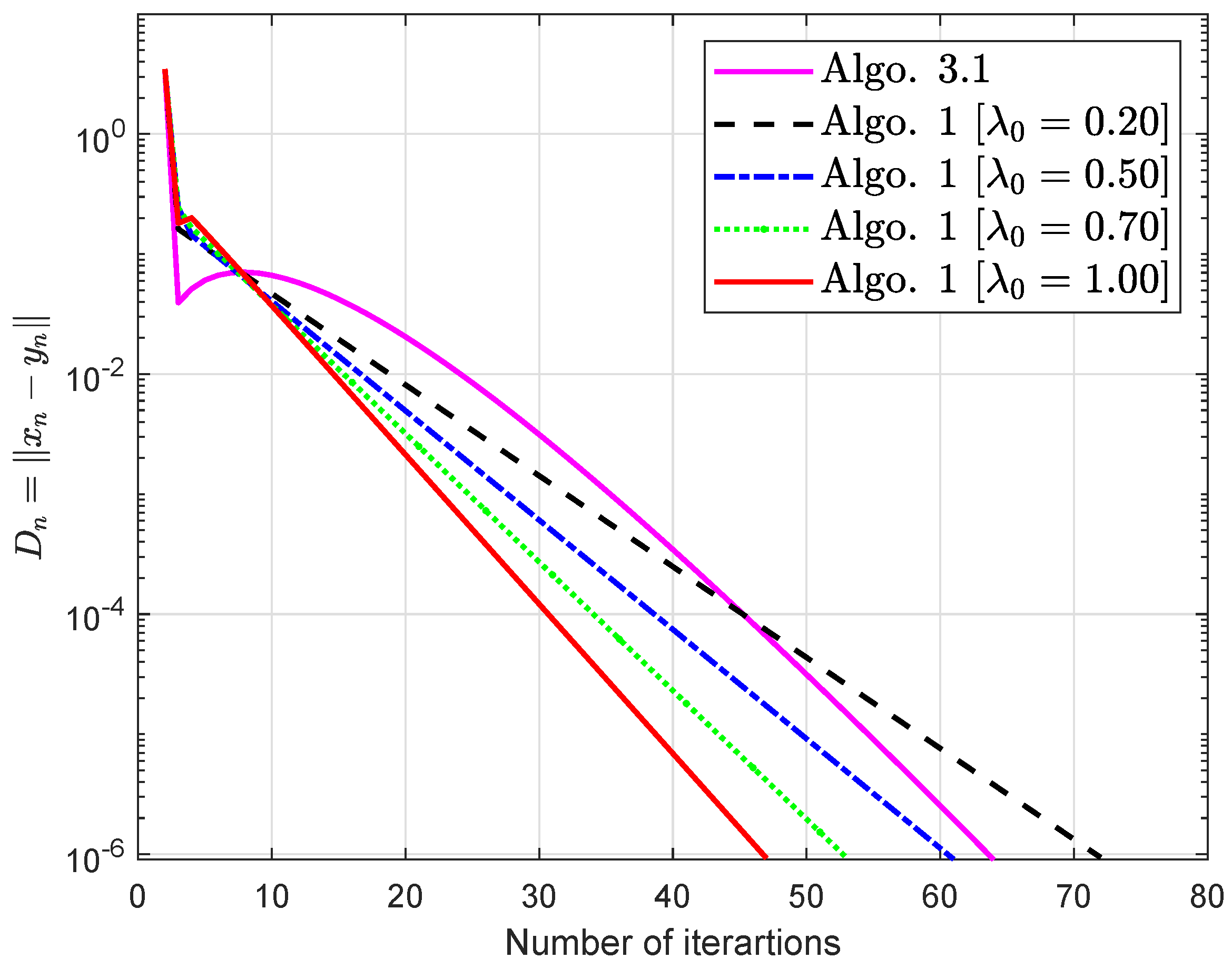
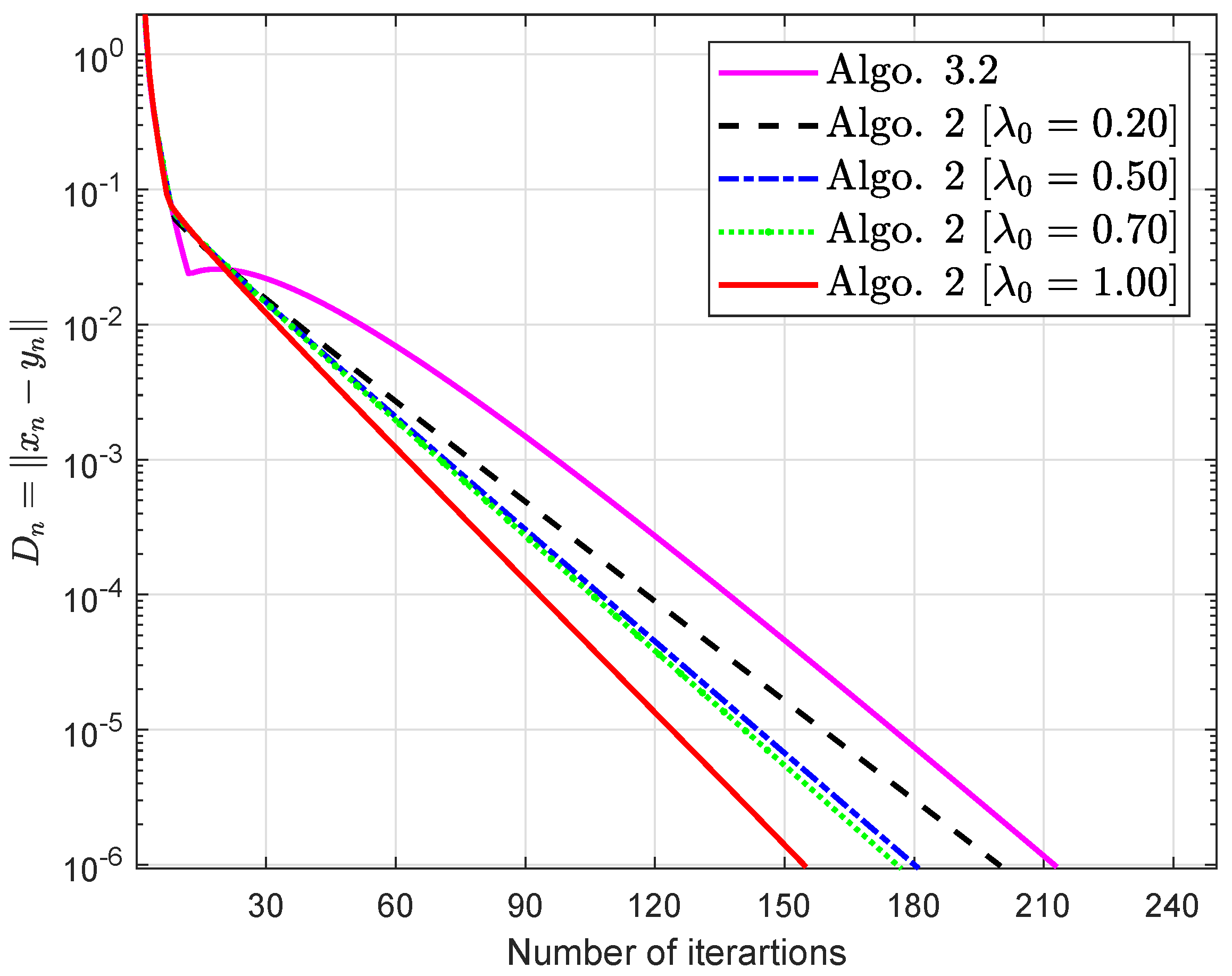
5. Numerical Illustration

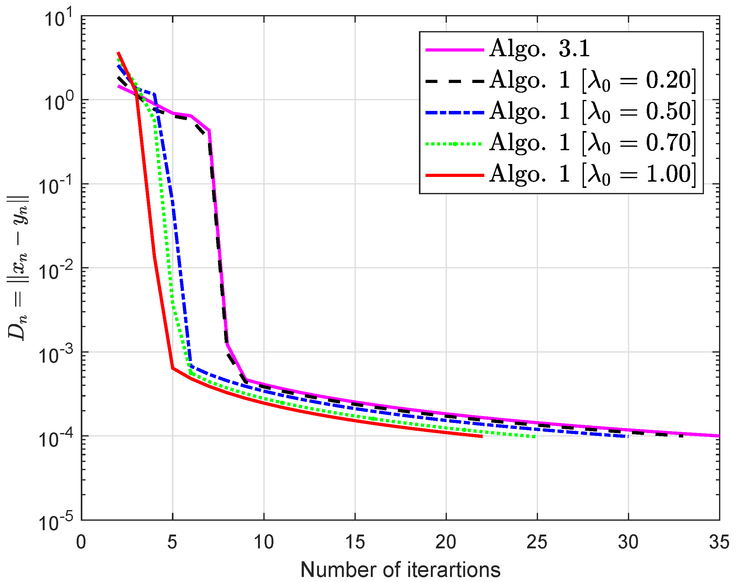
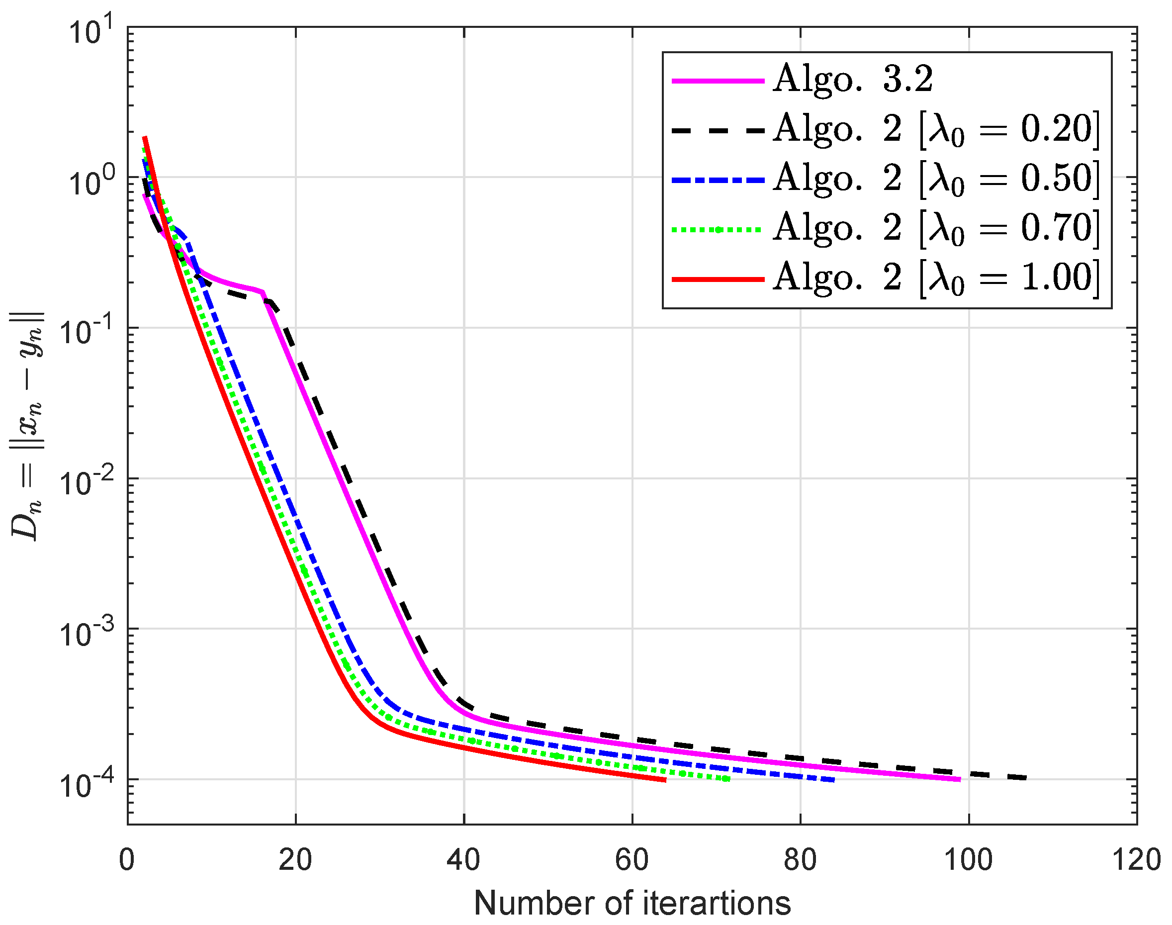
The computational results in this section show that our proposed algorithms are more efficient than Algorithms 3.1 and 3.2 in [32]. The MATLAB program was executed in MATLAB version 9.5 on a PC (with Intel(R) Core(TM)i3-4010U CPU @ 1.70 GHz 1.70 GHz, RAM 4.00 GB) (R2018b). In all our algorithms, we used the built-in MATLAB fmincon function to solve the minimization problems. (i) The setting for design variables for Algorithm 3.1 (Algo. 3.1) and Algorithm 3.2 (Algo. 3.2) in [32] possess different values that are given in all examples.

$${\varphi }_k=\frac{1}{40k},{\delta }_k=\frac{1}{10}+\frac{1}{10k},{\lambda }_k=\frac{k}{3+2c_1},{\phi }_k=\frac{1}{4}+\frac{1}{4n}\mathrm{and}{D}_k=\parallel s_k-m_k\parallel \le ϵ.$$

(ii) The settings for the design variables for Algorithm 1 (Algo. 1 ) and Algorithm 2 (Algo. 2) are

$${\varphi }_k=\frac{1}{40k},{\delta }_k=\frac{1}{10}+\frac{1}{10k},{\phi }_k=\frac{1}{4}+\frac{1}{4k},D_k=\parallel s_k-m_k\parallel \le ϵ\mathrm{and}\mathrm{for}\mathrm{different}{\lambda }_0.$$

Example 1.

Let us consider a bifunction $\mathcal{R}:\Sigma \times \Sigma \to \mathbb{R},$ which is represented as follows:

$$\mathcal{R}(s,m)=\sum _{i=2}^5(m_i-s_i)\parallel s\parallel ,\forall s,m\in {\mathbb{R}}^5.$$

In addition, the convex set is defined as follows:

$$\Sigma =\left\{(s_1,\dots ,s_5):s_1\ge -1,s_i\ge 1,i=2,\dots ,5\right\}.$$

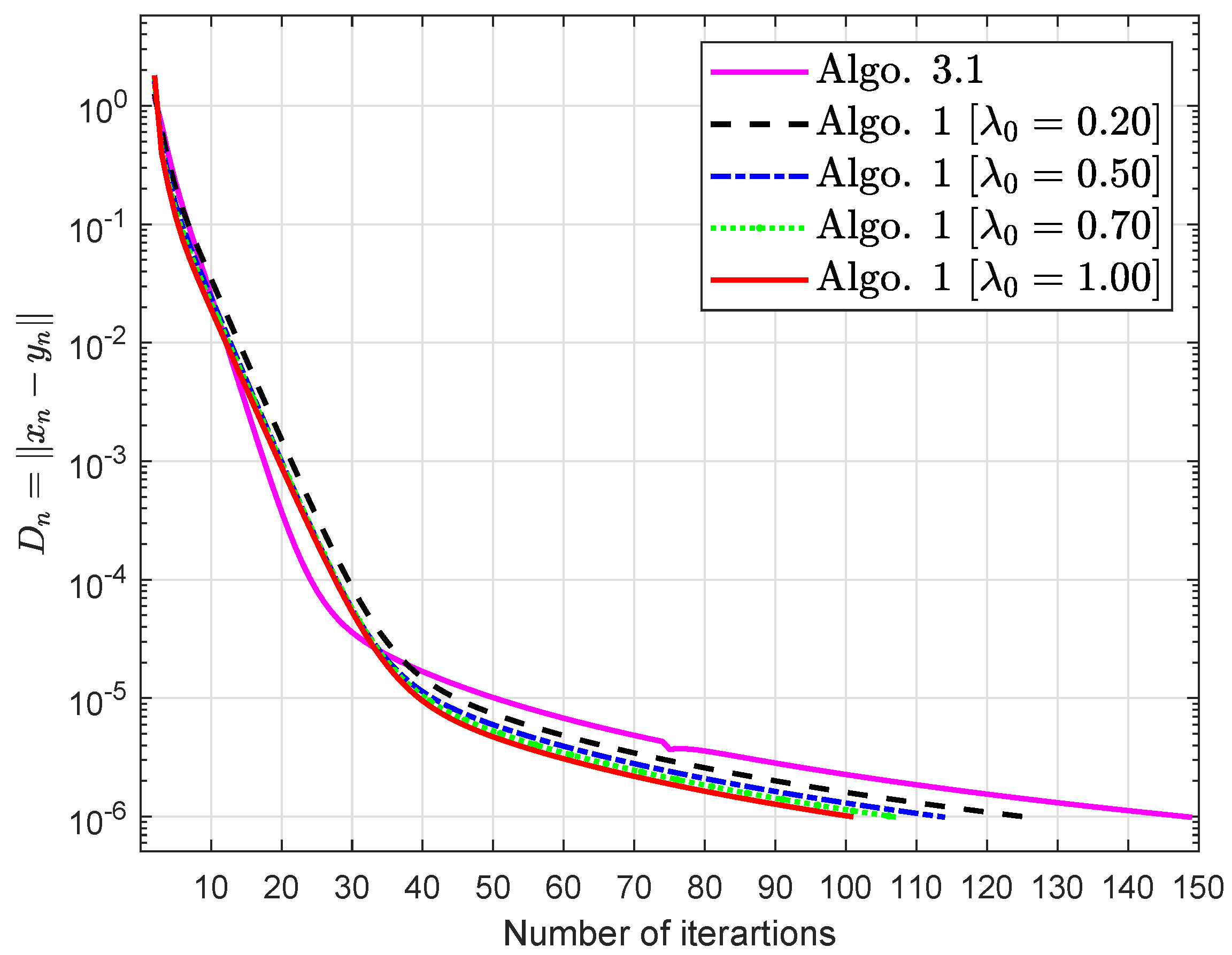
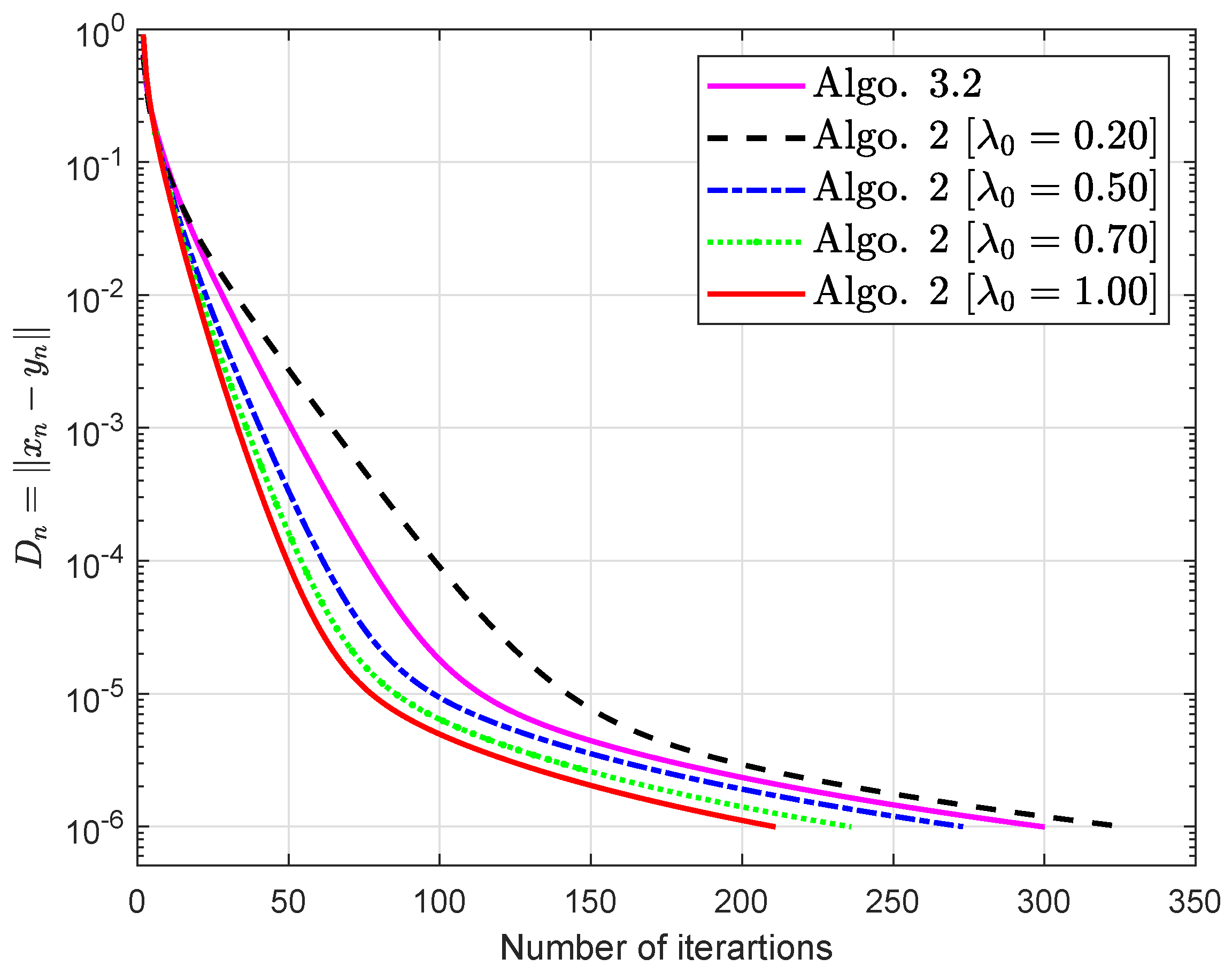
Consequently, $\mathcal{R}$ is Lipschitz-type continuous across $c_1=c_2=2$ and meets the condition($\mathcal{R}$1)–($\mathcal{R}$4). The obtained simulations are shown in Figure 1 and Figure 2 and

Table 1. Algorithm 1 is compared to Algorithm 3.1 in [32].

		Number of Iterations				CPU Time in Seconds
${\mathbf{\lambda }}_{\mathbf{0}}$		Algo. 3.1	Algo. 1			Algo. 3.1	Algo. 1
0.20		35	33			1.6799	1.6119
0.50		-	30			-	1.4787
0.70		-	25			-	1.1520
1.00		-	22			-	1.0100

and

Table 2. Algorithm 2 is compared to Algorithm 3.2 in [32].

		Number of Iterations				CPU Time in Seconds
${\mathbf{\lambda }}_{\mathbf{0}}$		Algo. 3.2	Algo. 2			Algo. 3.2	Algo. 2
0.20		99	109			4.9391	5.3081
0.50		-	84			-	4.0511
0.70		-	72			-	3.2269
1.00		-	64			-	2.9225

by using $s_1=(2,3,2,5,5)$ and $ϵ={10}^{-4}.$

Example 2.

According to the articles [29], the bifunction $\mathcal{R}$ might be written as follows:

$$\mathcal{R}(s,m)=\langle As+Bm+c,m-s\rangle ,$$

where $c\in {\mathbb{R}}^5$ and A, B are

$$A=\left(\begin{array}{ccccc}3.1& 2& 0& 0& 0\\ 2& 3.6& 0& 0& 0\\ 0& 0& 3.5& 2& 0\\ 0& 0& 2& 3.3& 0\\ 0& 0& 0& 0& 3\end{array}\right)B=\left(\begin{array}{ccccc}1.6& 1& 0& 0& 0\\ 1& 1.6& 0& 0& 0\\ 0& 0& 1.5& 1& 0\\ 0& 0& 1& 1.5& 0\\ 0& 0& 0& 0& 2\end{array}\right)c=\left(\begin{array}{c}1\\ -2\\ -1\\ 2\\ -1\end{array}\right).$$

The Lipschitz parameters are also $c_1=c_2=\frac{1}{2}\parallel A-B\parallel$ (see [29]). The possible set Σ and its subset ${\mathbb{R}}^5$ are given as

$$\Sigma :=\{s\in {\mathbb{R}}^5:-5\le s_i\le 5\}.$$

Figure 3 and Figure 4 and

Table 3. Algorithm 1 is compared to Algorithm 3.1 in [32].

		Number of Iterations				CPU Time in Seconds
${\mathbf{\lambda }}_{\mathbf{0}}$		Algo. 3.1	Algo. 1			Algo. 3.1	Algo. 1
0.20		149	126			7.0363	5.7321
0.50		-	114			-	5.0527
0.70		-	107			-	4.8159
1.00		-	101			-	4.5495

and

Table 4. Algorithm 2 is compared to Algorithm 3.2 in [32].

		Number of Iterations				CPU Time in Seconds
${\mathbf{\lambda }}_{\mathbf{0}}$		Algo. 3.2	Algo. 2			Algo. 3.2	Algo. 2
0.20		300	326			14.7791	14.2233
0.50		-	273			-	13.7107
0.70		-	236			-	11.7754
1.00		-	211			-	11.2054

display the numeric effects with $s_1=(1,\dots ,1)$ and $ϵ={10}^{-6}.$

Example 3.

Consider that $\Pi =L^2\left([0,1]\right)$ is indeed a Hilbert space with

$$\parallel s\parallel =\sqrt{{\int }_0^1{\left|s\left(t\right)\right|}^{2}dt},$$

where the internal product

$$\langle s,m\rangle ={\int }_0^{1}s\left(t\right)m\left(t\right)dt,\forall s,m\in \Pi .$$

Suppose that unit ball is $\Sigma :=\{s\in L^2\left([0,1]\right):\parallel s\parallel \le 1\}.$ Let us begin by defining an operator

$$G\left(s\right)\left(t\right)={\int }_0^1\left(s\left(t\right)-H(t,s)\mathcal{R}\left(s\right(s\left)\right)\right)ds+g\left(t\right),$$

where

$$H(t,s)=\frac{2ts{e}^{(t+s)}}{e\sqrt{e^2-1}},\mathcal{R}\left(s\right)=cosx,g\left(t\right)=\frac{2t{e}^t}{e\sqrt{e^2-1}}.$$

As illustrated in [45], G is monotone and L-Lipschitz-continuous via $L=2.$ Figure 5 and Figure 6 and

Table 5. Algorithm 1 is compared to Algorithm 3.1 in [32].

		Number of Iterations				CPU Time in Seconds
${\mathbf{\lambda }}_{\mathbf{0}}$		Algo. 3.1	Algo. 1			Algo. 3.1	Algo. 1
0.20		64	72			0.0174	0.0331
0.50		–	61			–	0.0295
0.70		–	53			–	0.0273
1.00		–	47			–	0.0265

and

Table 6. Algorithm 2 is compared to Algorithm 3.2 in [32].

		Number of Iterations				CPU Time in Seconds
${\mathbf{\lambda }}_{\mathbf{0}}$		Algo. 3.2	Algo. 2			Algo. 3.2	Algo. 2
0.20		213	200			0.0313	0.0500
0.50		–	181			–	0.0460
0.70		–	177			–	0.0352
1.00		–	155			–	0.0260

illustrate the numerical results with $s_1=t$ and $ϵ={10}^{-6}.$

Discussion About Numerical Experiments: The following conclusions may be drawn from the numerical experiments outlined above: (i) Examples 1–3 have reported data for numerous methods in both finite- and infinite-dimensional domains. It is apparent that the given algorithms outperformed in terms of number of iterations and elapsed time in practically all circumstances. All trials demonstrate that the suggested algorithms outperform the previously available techniques. (ii) Examples 1–3 have reported results for several methods in finite and infinite-dimensional domains. In most cases, we can observe that the scale of the problem and the relative standard deviation used impact the algorithm’s effectiveness. (iii) The development of an inappropriate variable step size generates a hump in the graph of algorithms in all examples. It has no impact on the effectiveness of the algorithms. (iv) For large-dimensional problems, all approaches typically took longer and showed significant variation in execution time. The number of iterations, on the other hand, changes slightly less.

6. Conclusions

The paper provides two explicit extragradient-like approaches for solving an equilibrium problem involving a pseudomonotone and a Lipschitz-type bifunction in a real Hilbert space. A new step-size rule has been presented that does not rely on Lipschitz-type constant information. The algorithm’s convergence has been established. Several tests are presented to show the numerical behavior of our two algorithms and to compare them to others that are well known in the literature.

References

1. Blum, E. From optimization and variational inequalities to equilibrium problems. Math. Stud. 1994, 63, 123–145. [Google Scholar]
2. Fan, K. A Minimax Inequality and Applications, Inequalities III; Shisha, O., Ed.; Academic Press: New York, NY, USA, 1972. [Google Scholar]
3. Bigi, G.; Castellani, M.; Pappalardo, M.; Passacantando, M. Existence and solution methods for equilibria. Eur. J. Oper. Res. 2013, 227, 1–11. [Google Scholar] [CrossRef] [Green Version]
4. Muu, L.; Oettli, W. Convergence of an adaptive penalty scheme for finding constrained equilibria. Nonlinear Anal. Theory Methods Appl. 1992, 18, 1159–1166. [Google Scholar] [CrossRef]
5. Hung, P.G.; Muu, L.D. The Tikhonov regularization extended to equilibrium problems involving pseudomonotone bifunctions. Nonlinear Anal. Theory Methods Appl. 2011, 74, 6121–6129. [Google Scholar] [CrossRef]
6. Konnov, I. Application of the Proximal Point Method to Nonmonotone Equilibrium Problems. J. Optim. Theory Appl. 2003, 119, 317–333. [Google Scholar] [CrossRef]
7. Moudafi, A. Proximal point algorithm extended to equilibrium problems. J. Nat. Geom. 1999, 15, 91–100. [Google Scholar]
8. Oliveira, P.; Santos, P.; Silva, A. A Tikhonov-type regularization for equilibrium problems in Hilbert spaces. J. Math. Anal. Appl. 2013, 401, 336–342. [Google Scholar] [CrossRef]
9. Rehman, H.U.; Kumam, P.; Shutaywi, M.; Pakkaranang, N.; Wairojjana, N. An Inertial Extragradient Method for Iteratively Solving Equilibrium Problems in Real Hilbert Spaces. Int. J. Comput. Math. 2021, 99, 1081–1104. [Google Scholar] [CrossRef]
10. Rehman, H.u.; Pakkaranang, N.; Hussain, A.; Wairojjana, N. A modified extra-gradient method for a family of strongly pseudomonotone equilibrium problems in real Hilbert spaces. J. Math. Comput. Sci. 2021, 22, 38–48. [Google Scholar] [CrossRef]
11. Wairojjana, N.; Pakkaranang, N.; Pholasa, N. Strong convergence inertial projection algorithm with self-adaptive step size rule for pseudomonotone variational inequalities in Hilbert spaces. Demonstr. Math. 2021, 54, 110–128. [Google Scholar] [CrossRef]
12. Rehman, H.U.; Kumam, P.; Abubakar, A.B.; Cho, Y.J. The extragradient algorithm with inertial effects extended to equilibrium problems. Comput. Appl. Math. 2020, 39, 100. [Google Scholar] [CrossRef]
13. Rehman, H.U.; Kumam, P.; Kumam, W.; Shutaywi, M.; Jirakitpuwapat, W. The Inertial Sub-Gradient Extra-Gradient Method for a Class of Pseudo-Monotone Equilibrium Problems. Symmetry 2020, 12, 463. [Google Scholar] [CrossRef] [Green Version]
14. Konnov, I.V. Regularization method for nonmonotone equilibrium problems. J. Nonlinear Convex Anal. 2009, 10, 93–101. [Google Scholar]
15. Konnov, I.V. Partial proximal point method for nonmonotone equilibrium problems. Optim. Methods Softw. 2006, 21, 373–384. [Google Scholar] [CrossRef]
16. Singh, A.; Shukla, A.; Vijayakumar, V.; Udhayakumar, R. Asymptotic stability of fractional order (1,2] stochastic delay differential equations in Banach spaces. Chaos Solitons Fractals 2021, 150, 111095. [Google Scholar] [CrossRef]
17. Patel, R.; Shukla, A.; Jadon, S.S. Existence and optimal control problem for semilinear fractional order (1,2] control system. Math. Methods Appl. Sci. 2020. [Google Scholar] [CrossRef]
18. Shukla, A.; Sukavanam, N.; Pandey, D. Controllability of Semilinear Stochastic System with Multiple Delays in Control. IFAC Proc. Vol. 2014, 47, 306–312. [Google Scholar] [CrossRef] [Green Version]
19. Shukla, A.; Patel, R. Existence and Optimal Control Results for Second-Order Semilinear System in Hilbert Spaces. Circuits Syst. Signal Process. 2021, 40, 4246–4258. [Google Scholar] [CrossRef]
20. Van Hieu, D.; Duong, H.N.; Thai, B. Convergence of relaxed inertial methods for equilibrium problems. J. Appl. Numer. Optim. 2021, 3, 215–229. [Google Scholar]
21. Ogbuisi, F.U. The projection method with inertial extrapolation for solving split equilibrium problems in Hilbert spaces. Appl. Set-Valued Anal. Optim. 2021, 3, 239–255. [Google Scholar]
22. Liu, L.; Cho, S.Y.; Yao, J.C. Convergence Analysis of an Inertial Tseng’s Extragradient Algorithm for Solving Pseudomonotone Variational Inequalities and Applications. J. Nonlinear Var. Anal. 2021, 5, 627–644. [Google Scholar]
23. Rehman, H.u.; Kumam, P.; Argyros, I.K.; Shutaywi, M.; Shah, Z. Optimization Based Methods for Solving the Equilibrium Problems with Applications in Variational Inequality Problems and Solution of Nash Equilibrium Models. Mathematics 2020, 8, 822. [Google Scholar] [CrossRef]
24. Rehman, H.u.; Kumam, P.; Shutaywi, M.; Alreshidi, N.A.; Kumam, W. Inertial Optimization Based Two-Step Methods for Solving Equilibrium Problems with Applications in Variational Inequality Problems and Growth Control Equilibrium Models. Energies 2020, 13, 3292. [Google Scholar] [CrossRef]
25. Rehman, H.; Kumam, P.; Dong, Q.-L.; Peng, Y.; Deebani, W. A new Popov’s subgradient extragradient method for two classes of equilibrium programming in a real Hilbert space. Optimization 2020, 70, 2675–2710. [Google Scholar] [CrossRef]
26. Rehman, H.U.; Pakkaranang, N.; Kumam, P.; Cho, Y.J. Modified subgradient extragradient method for a family of pseudomonotone equilibrium problems in real a Hilbert space. J. Nonlinear Convex Anal. 2020, 21, 2011–2025. [Google Scholar]
27. Flåm, S.D.; Antipin, A.S. Equilibrium programming using proximal-like algorithms. Math. Program. 1996, 78, 29–41. [Google Scholar] [CrossRef]
28. Korpelevich, G. The extragradient method for finding saddle points and other problems. Matecon 1976, 12, 747–756. [Google Scholar]
29. Tran, D.Q.; Dung, M.L.; Nguyen, V.H. Extragradient algorithms extended to equilibrium problems. Optimization 2008, 57, 749–776. [Google Scholar] [CrossRef]
30. Hieu, D.V.; Quy, P.K.; Vy, L.V. Explicit iterative algorithms for solving equilibrium problems. Calcolo 2019, 56, 11. [Google Scholar] [CrossRef]
31. Yang, J.; Liu, H.; Liu, Z. Modified subgradient extragradient algorithms for solving monotone variational inequalities. Optimization 2018, 67, 2247–2258. [Google Scholar] [CrossRef]
32. Wang, S.; Zhang, Y.; Ping, P.; Cho, Y.; Guo, H. New extragradient methods with non-convex combination for pseudomonotone equilibrium problems with applications in Hilbert spaces. Filomat 2019, 33, 1677–1693. [Google Scholar] [CrossRef] [Green Version]
33. Censor, Y.; Gibali, A.; Reich, S. The Subgradient Extragradient Method for Solving Variational Inequalities in Hilbert Space. J. Optim. Theory Appl. 2010, 148, 318–335. [Google Scholar] [CrossRef] [PubMed] [Green Version]
34. Tiel, J.V. Convex Analysis: An Introductory Text, 1st ed.; Wiley: New York, NY, USA, 1984. [Google Scholar]
35. Bushell, P.J. UNIFORM CONVEXITY, HYPERBOLIC GEOMETRY, AND NONEXPANSIVE MAPPINGS (Pure and Applied Mathematics: A Series of Monographs & Textbooks, 83) By K. Goebel and S. Reich: Pp. 192. SFr.96.-. (Marcel Dekker Inc, U.S.A., 1984). Bull. Lond. Math. Soc. 1985, 17, 293–294. [Google Scholar] [CrossRef]
36. Kreyszig, E. Introductory Functional Analysis with Applications, 1st ed.; Wiley Classics Library, Wiley: Hoboken, NJ, USA, 1989. [Google Scholar]
37. Bauschke, H.H.; Combettes, P.L. Convex Analysis and Monotone Operator Theory in Hilbert Spaces, 2nd ed.; CMS Books in Mathematics; Springer International Publishing: Berlin/Heidelberg, Germany, 2017. [Google Scholar]
38. Xu, H.K. Another control condition in an iterative method for nonexpansive mappings. Bulletin of the Australian Mathematical Society 2002, 65, 109–113. [Google Scholar] [CrossRef] [Green Version]
39. Maingé, P.E. Strong Convergence of Projected Subgradient Methods for Nonsmooth and Nonstrictly Convex Minimization. Set-Valued Anal. 2008, 16, 899–912. [Google Scholar] [CrossRef]
40. Bianchi, M.; Schaible, S. Generalized monotone bifunctions and equilibrium problems. J. Optim. Theory Appl. 1996, 90, 31–43. [Google Scholar] [CrossRef]
41. Mastroeni, G. On Auxiliary Principle for Equilibrium Problems. In Nonconvex Optimization and Its Applications; Springer: Boston, MA, USA, 2003; pp. 289–298. [Google Scholar] [CrossRef]
42. Rehman, H.U.; Kumam, P.; Cho, Y.J.; Yordsorn, P. Weak convergence of explicit extragradient algorithms for solving equilibirum problems. J. Inequalities Appl. 2019, 2019, 282. [Google Scholar] [CrossRef]
43. Browder, F.; Petryshyn, W. Construction of fixed points of nonlinear mappings in Hilbert space. J. Math. Anal. Appl. 1967, 20, 197–228. [Google Scholar] [CrossRef] [Green Version]
44. Rehman, H.U.; Kumam, P.; Je Cho, Y.; Suleiman, Y.I.; Kumam, W. Modified Popov’s explicit iterative algorithms for solving pseudomonotone equilibrium problems. Optim. Methods Softw. 2020, 36, 82–113. [Google Scholar] [CrossRef]
45. Van Hieu, D.; Anh, P.K.; Muu, L.D. Modified hybrid projection methods for finding common solutions to variational inequality problems. Comput. Optim. Appl. 2017, 66, 75–96. [Google Scholar] [CrossRef]
Figure 1. Algorithm 1 is compared to Algorithm 3.1 in [32].
Symmetry 14 01045 g001
Figure 2. Algorithm 2 is compared to Algorithm 3.2 in [32].
Symmetry 14 01045 g002
Figure 3. Algorithm 1 is compared to Algorithm 3.1 in [32].
Symmetry 14 01045 g003
Figure 4. Algorithm 2 is compared to Algorithm 3.2 in [32].
Symmetry 14 01045 g004
Figure 5. Algorithm 1 is compared to Algorithm 3.1 in [32].
Symmetry 14 01045 g005
Figure 6. Algorithm 2 is compared to Algorithm 3.2 in [32].
Symmetry 14 01045 g006