
Robust Optimum Life-Testing Plans under Progressive Type-I Interval Censoring Schemes with Cost Constraint


1
School of Statistics and Information, Shanghai University of International Business and Economics, Shanghai 201613, China
2
School of Statistics and Mathematics, Shanghai Lixin, University of Accounting and Finance, Shanghai 201620, China
3
College of Mathematics and Science, Shanghai Normal University, Shanghai 201418, China
*
Author to whom correspondence should be addressed.
Symmetry 2022, 14(5), 1047; https://0-doi-org.brum.beds.ac.uk/10.3390/sym14051047
Submission received: 12 April 2022
/
Revised: 15 May 2022
/
Accepted: 17 May 2022
/
Published: 19 May 2022
(This article belongs to the Special Issue Symmetrical and Asymmetrical Distributions in Statistics and Probability)
Abstract
:This paper considers optimal design problems for the Weibull distribution, which can be used to model symmetrical or asymmetrical data, in the presence of progressive interval censoring in life-testing experiments. Two robust approaches, Bayesian and minimax, are proposed to deal with the dependence of the D-optimality and c-optimality on the unknown model parameters. Meanwhile, the compound design method is applied to ensure a compromise between the precision of estimation of the model parameters and the precision of estimation of the quantiles. Furthermore, to make the design become more practical, the cost constraints are taken into account in constructing the optimal designs. Two algorithms are provided for finding the robust optimal solutions. A simulated example and a real life example are given to illustrate the proposed methods. The sensitivity analysis is also studied. These new design methods can help the engineers to obtain robust optimal designs for the censored life-testing experiments.
1. Introduction
Progressive censoring is frequently employed in life-testing experiments because it permits removing the test units at the points other than the final termination point, which can save experiment time and/or cost. Recently, the research on progressive censoring has grown very fast. For the relevant research progress one may refer to two important monographs (Balakrishnan et al. [1]; Balakrishnan and Cramer [2]) and the review article (Balakrishnan [3]). In applications, progressive type-I and type-II censoring are two important types of progressive censoring schemes. They are usually required to continuously observe the testing process under a given censoring scheme. However, due to the high cost and/or possible danger, it is sometimes infeasible to carry out continuous inspection in monitoring the test. Alternatively, an interval inspection scheme can be used, where only the number of failures between two consecutive inspections is recorded. Combining the concepts of the progressive censoring and the interval censoring, Aggarwala [4] developed a progressive type-I interval censoring (PIC-I) scheme.
Since Aggarwala [4], many scholars have studied the statistical inference for PIC-I data under various life distributions by the maximum likelihood method and/or Bayesian method. Some of them are Xiang and Tse [5], Ng and Wang [6], Chen and Lio [7], Lin and Lio [8], Singh and Tripathi [9], Lodhi and Tripathi [10], Budhiraja and Pradhan [11], Wu and Chang [12], and Alotaibi et al. [13]. In addition to statistical inference, many researchers have been focused on optimally obtaining PIC-I test plans. For more information on this direction one can refer to, e.g., Wu et al. [14], Lin et al. [15], Lin et al. [16], Singh and Tripathi [9], Roy and Pradhan [17], Budhiraja and Pradhan [18], Roy and Pradhan [19], and Wu et al. [20].
In most of the aforementioned studies on designing PIC-I test schemes, the model parameters that appear in the design criteria are assumed to be known, usually gained from previous studies. Designs obtained under these planning values are called locally optimal designs. If these values are uncertain, which is usually the case, or are incorrectly specified, then these designs may not be optimal. Therefore, it would be helpful for researchers to obtain the optimal designs, which are robust against misspecifications of the values of the model parameters. For the PIC-I life tests, Roy and Pradhan [17,19] proposed to employ proper prior distributions over the entire parameter space to describe the knowledge about the parameters. Then the designs obtained were called Bayesian optimal designs. Unfortunately, we sometimes do not have enough information to construct such prior distributions. In this case, the minimax method can be used to obtain robust designs. The resulting design is often referred to as the minimax optimal design. In fact, in the literature of experimental design, the Bayesian and minimax strategies have been widely used to overcome the dependency of the optimal design on the unknown parameters (see, e.g., Chaloner and Verdinelli [21], Atkinson, et al. [22], and Yue and Zhou [23]). However, in our knowledge, these problems have not been properly addressed when designing the reliability test.
Previous reviewed studies mainly focused on single design objective, such as estimation of model parameters (e.g., Wu et al. [14]) or the qth quantile of the life distribution or minimization of the total cost of life testing (e.g., Roy and Pradhan [19]). However, sometimes researchers prefer to achieve a design that meets multiple objectives at the same time. This design is called a multiple-objective design, which is robust with respect to the design objectives. In the accelerated life test (ALT), Pan and Yang [24] proposed a compound design criterion to obtain a dual-objective optimal design, which could make a trade-off between the model parameter estimation and the model-based prediction. Bhattacharya et al. [25] gave a new design method based on multi-criteria, taking variance and cost factors into account in the context of the hybrid censored life-testing experiment. Though there are some studies on robust designs in reliability life tests for multiple design objectives, robust optimum designs for PIC-I tests have received little attention in the literature so far.
In this paper, we study robust optimum designs for PIC-I life tests by using the Bayesian and minimax strategies to deal with the model parameters dependency problem and the compound design method to fulfill multiple design objectives. Two robust optimum design criteria and two algorithms are provided to calculate robust optimum designs when the experimental cost is taken into account. Our methods can help practitioners have easier access to robust optimum designs when the model parameters are uncertain and there are more than one design objective, and can be easily extended to obtain robust designs for other test schemes.
The rest of this paper is organized as follows. Section 2 introduces the PIC-I test plan and derives the Fisher information matrix (FIM). Section 3 provides definitions of the Bayesian compound and the minimax compound optimality criteria for the PIC-I test plans based on both D-optimality and c-optimality, termed -optimality and -optimality, respectively. Section 4 presents two optimization algorithms, i.e., mixed-integer nonlinear optimization (MNO) and Particle swarm optimization (PSO), to derive optimal equal spaced PIC-I test plans and general PIC-I test plans, respectively. Numerical results are given in Section 5 and Section 6 to illustrate the proposed methods. Conclusions and discussions are made in Section 7.
2. Preliminaries
Suppose that the lifetime T of a test product follows the Weibull distribution with the probability density function (pdf)
and the cumulative distribution function (cdf)
Let . We can convert the Weibull distribution to the extreme value (Gumbel) distribution given by
where is the location parameter and is the scale parameter. The corresponding cdf can be written as
Assume that a PIC-I scheme is employed, where all N units are simultaneously placed on a life test at the beginning of the experiment, and interval inspections are conducted at time points . At the jth inspection time , failed units are observed and surviving units are randomly removed from the experiment. Let denote the probability that a unit fails in the jth time interval given that the failure has not occurred in an earlier time interval, i.e.,
where , with and .
Under the PIC-I test plan, the distribution of the number of failed units is binomial, i.e.,
where and is the number of non-removed surviving units at the beginning of the jth inspection. Note that the number of removal units is a random variable due to the randomness of the variable , and its value can be computed through the predetermined percentages of the remaining survived units (with ). That is, . All data collected from the PIC-I test plan are denoted by .
Let be the vector of the model parameters. Based on the data and the cdf given in Equation (4), the likelihood function of can be written as
Then, the corresponding log-likelihood function is
Therefore, the maximum likelihood estimates (MLEs) of the parameters and can be obtained by solving the following likelihood equations:
Furthermore, the FIM of the parameters can be written as
where
and . Here, , and is the survival probability of the test unit until the time point . Under some mild regularity conditions, the FIM is approximate to the inverse of the variance-covariance matrix of the MLE of .
3. Robust PIC-I Test Plan
3.1. PIC-I Test Plan
In this section, we investigate the optimal PIC-I test plan with limited cost constraint. Generally, the PIC-I test plan consists of the total number of test units N, the number of inspections k, the inspection time points and the proportions of the removals at each time point . For convenience, we denote the PIC-I test plan as , i.e.,
From the expression of the FIM given in (8), it can be easily concluded that if there is no limit on the removal proportions and if the other conditions are fixed, the optimal choices of are zeros. Some evidences can be found in the work by Roy and Pradhan [17,19]. However, this is not consistent with the topic discussed in this paper. To investigate the influence of the removal proportions on the optimal PIC-I test plan, we assume that the scheme of removals at each points is predetermined. Then, the PIC-I test plan can be re-expressed as
where is the set of positive integers, is the set of positive natural number, is the set of possible values of and will be predetermined by the experimenter.
For practical convenience, many studies assume that the inspection time intervals have equal lengths, say . Then, the inspection time points can be re-expressed as where is the maximum number of inspections. In addition, the removal proportions at each inspection times can be assumed constant, i.e., . Therefore, the design (9) can be reduced to
Since the FIM given in (8) depends not only on the parameter vector , but also the design , we denote by in what follows.
3.2. D- and c-Optimal Design Criteria
The first design criterion we considered is the D-optimality for estimating the model parameter vector as efficiently as possible. The D-optimal criterion is defined as follows:
where are given in Equation (8).
Let be the set consisting of all possible designs in the form of (9) or (10). The design , which satisfies for given is called a D-optimal design. The rationality of taking use of this design criterion can be found in Atkinson et al. [22] and has been discussed by many authors (e.g., Wu et al. [14], and Roy and Pradhan [17]).
In addition to the estimation of the model parameters and , an experimenter may also be interested in estimating the qth quantile lifetime of the units (Roy and Pradhan [19]). Let be the logarithm of the qth quantile lifetime of the units, and . Under the distribution (4), then can be written as . By the invariance property of the MLE and the delta method, the distribution of the estimator is approximately normal with mean and variance . To efficiently estimate , the following c-optimality criterion is usually adopted:
A design which minimizes for given and q over the design space is called a c-optimal design.
Remark 1.
To compare the optimal PIC-I test plan with another arbitrary test plan under a given L-optimality criterion (), we define the following efficiency function
3.3. Bayesian Compound Design Criterion
Note that the design criteria and depend not only on the design , but also on the the parameters . Optimal designs obtained under a perfect guess (planning) values are called locally optimal designs (Chernoff [27]). Numerical results given in Wu et al. [14] indicate that D-optimal test plans depend on the setting of the parameters and . To reduce the risks caused by misspecifying the planning values , many approaches, such as the Bayesian, minimax, adaptive, or sequential approaches have been proposed in the literature of optimal experimental designs, see Atkinson et al. [22] for details. However, planning robust test schemes has rarely been found in a reliability study. Therefore, in the following part of this subsection, we apply robust design techniques to obtain robust PIC-I test plans. To be consistent with most experiments in practical applications, we confine ourselves on the static robust design methods, including the Bayesian and the minimax approaches to obtain robust test plans against the uncertainty of the parameters .
In addition, even when all parameters in the D-optimality and c-optimality criteria have the same settings, the D-optimal design and the c-optimal design are not necessarily identical, see the numerical results listed in Table 1. To get a good test plan that satisfies many design objectives, the compound design criterion (Cook and Wong [28]) should be a good choice. It can ensure that the optimal design has good performances for different design purposes (Pan and Yang [24]). Therefore, considering the uncertainty of the parameters in the model and two possible design objectives, we propose the Bayesian compound optimality criterion (termed -optimality), which is given as follows:
where is the prior over the set , which will be specified later, and is the weight parameter reflecting the relative importance between the D-optimality and the c-optimality. A design, , which minimizes over the design space is called a -optimal design. In this paper, we assume that the prior of is a censored normal distribution over the interval , and its pdf is
where and are the pdf and cdf of the normal distribution and are the hyperparameters predetermined by the experimenter. The prior of the scale parameter is assumed to be a censored inverse over the interval with the pdf
where and are the pdf and cdf of the inverse Gamma distribution , respectively, and are the hyperparameters predetermined by the experimenter. Under the assumption of the priors of and being independent, the joint prior density of and is given as
In addition, when the weight equals 0 (or 1), then the -optimal design will reduce to Bayesian c (or D)-optimal design and be denoted as (or ). In the special case that the prior has only one support point , the -optimal design becomes the locally -optimal design, which can be denoted as and the corresponding design criterion is
To deal with the integration in the Bayesian optimality criterion, we can draw Q samples from the joint prior distribution and use the MCMC method to obtain the approximation of the Bayesian optimality criterion (14) (Roy and Pradhan [17,19]), i.e.,
However, the computational burden for this approximation will increase rapidly with the sample size Q. To reduce computational burden, Foo and Duffull [29] proposed a hypercube D-optimality criterion to optimize the logarithm of the product of the normalized determinants of FIM over the set of their model parameters, which consists of the combinations of the 2.5th and 97.5th percentiles of the priors distributions. In this paper, we utilize a similar idea to alleviate the computational burden, but more percentiles of the prior parameter distribution are used to ensure the accuracy of approximation. We denote the set of all combinations of these percentiles by . Then
3.4. Minimax Compound PIC-I Test Plan
Another popular robust design approach is the minimax method, which aims at finding the design that minimizes the maximum values of the compound optimality criterion over the parameters space . Similar to the Bayesian optimality criterion, the minimax optimality criterion (termed -optimality) is defined as follows:
where is the weight parameter similar as . The design minimizing over the design space is called a -optimal design. In addition, when the weight equals 0 (or 1), then the -optimal design will reduce to the minimax c-optimal design and be denoted as (or ).
3.5. Cost Constraint
To make the test plan be more practical for experimenters, we take the budget of the experiment into account at the planning stage. For the general design defined in Equation (9), we assume that there is a restriction on the total cost
where is the cost of one test unit, is the cost of one inspection, is the operation cost of one unit time, and C is the total cost. For more details one can refer to Wu et al. [14]. Furthermore, for the special test plan defined in (10), the cost constraint is defined as follows:
4. Algorithms
4.1. Mixed-Integer Nonlinear Optimization Algorithm
In this subsection, we give an algorithm inspired by Wu et al. [14] to search for the robust PIC-I test plan with equal inspection intervals of length and the constant removal proportion p, except at the end of the experiment. The design is given in (10) and the cost constraint is presented in (20). For clarity, we rewrite the robust design criteria and by and , respectively. Then, the optimization problem can be expressed as
Since , we have . Thus, the upper bound of N is obtained. Because the D-optimality and c-optimality are decreasing functions of N, we substitute N by its upper bound in the design criteria. Furthermore, for a given value of N, we have . Then the upper bound of k is . Similarly, we can obtain the upper bound of , for a given k. Therefore, the algorithm to solve the optimization problem (21) is given in Algorithm 1.
| Algorithm 1 MNO Algorithm. |
|
4.2. Particle Swarm Optimization Algorithm
In Section 4.1, we have considered a special case of the PIC-I test plan and give an algorithm to obtain the robust test plan. However, the procedure depends on the cost function and the assumption of equal length of inspection interval and the same removal proportion. In this subsection, we give an algorithm to solve the general design problem defined as follows:
The concrete form of the design has been given in (9). From the definition of the cost function in (19), we have . The information given in (8) implies that more test units will provide more information. Therefore, we substitute N in (8) by the supreme value to solve the optimization problem (22). Then, the optimality criterion or is a function of , which are all continuous variables. To solve this continuous optimization problem with constraints, we use the PSO algorithm, which is a population based stochastic optimization method inspired by the social behavior of birds flocking or fish schooling. It was introduced by Eberhart and Kennedy [30], improved by many authors to deal with all kinds of optimization problems. It has shown high efficiency in finding optimal points in various disciplines (Poli et al. [31], Ruidas et al. [32,33]). The PSO algorithm is derivative-free. There are few tuning parameters required of the algorithm and the knowledge of good solutions is retained by all particles, and particles in the swarm share information between, which makes the algorithm easily escape from local minima and converge at a fast rate. Recently, different versions of PSO have been used to solve all kinds of optimal design problems (see Chen et al. [34], Zhou et al. [35], and Liu et al. [36]). In the following we give a summary of the PSO algorithm for completeness. For the sake of brevity and clarity, we vectorize the design and denote it by , and by denote the optimality criterion function or . The optimization problem (22) is rewritten as
Here, are real random numbers between 0 and 1, is the best candidate solution found for the ith particle, is the best candidate solution for the entire population particles, and , are the user defined coefficients which respectively control the inertia, the exploitive, and the explorative attributes of the particle motion.
5. Numerical Example
In this section, we present a numerical example to illustrate the applications of the proposed robust design methods. As in the study by Wu et al. [14], we use the algorithm given by Aggarwala [4] to generate data with and the predetermined removed proportions . Then the corresponding parameters in model (4) become . The generated data are presented in Table 2. Based on the data, we easily obtain the MLEs of and , and , and their standard errors and , respectively. To use the Bayesian or minimiax design criteria, we assume that the range of the values of and are and , respectively. The hyperparameters in the censored normal distribution are and , respectively. Similarly, the hyperparameters in the censored inverse distribution are assumed to be and , respectively, which implies that the mean of is and the variance is . The cost parameters are assumed as follows: /unit, , /10 h, and . In our numerical results, the set , where is the ith quantile of and is the jth quantile of , which are used to obtain the approximation of the -optimality criterion in (14) or to calculate the -optimality criterion in (18). We set in the - and -optimal design criteria. Since the -optimal PIC-I test plans are very similar to their corresponding -optimal ones, then we do not show the numerical -optimal PIC-I test plans in what follows to save space. We will give some concluding remarks in Section 6. The R codes, written to obtain the results in this paper, can be obtained from the authors upon request.
5.1. Locally Optimal PIC-I Test Plans
By Algorithm 1, we first compute the locally D- and c-optimal equal spaced (ES) PIC-I test plans (denoted as and , respectively) at the planning values and when the removal proportions are and , respectively.
In Equations (24) and (25), we also present the efficiencies of the Bayesian and minimax D- and c-optimal test plans with , which will be defined later. These efficiencies indicate that these robust designs perform well.
To assess the influence of the settings of the parameters and and the design criteria, the optimal PIC-I test plans under different parameters settings and removal proportions for different design criteria are computed, which are shown in Table 1. Comparing with the optimal test plans presented in Equations (24) and (25), we find that the settings of the planning values will have a great impact on the final designs, especially when the uncertainty of and encountered in the design stage becomes great—so do the removal proportions and design criteria. The efficiencies of the c- and D-optimal designs relative to the D- and c-optimal designs are also shown in Table 1. These efficiencies imply that the design purposes will have an effect on the finial designs. In addition, for some planning values, the c-optimal test plans can be very inefficient, whereas the D-optimal test plans perform well under the c-optimality in all cases considered here.
5.2. Bayesian Optimal PIC-I Test Plans
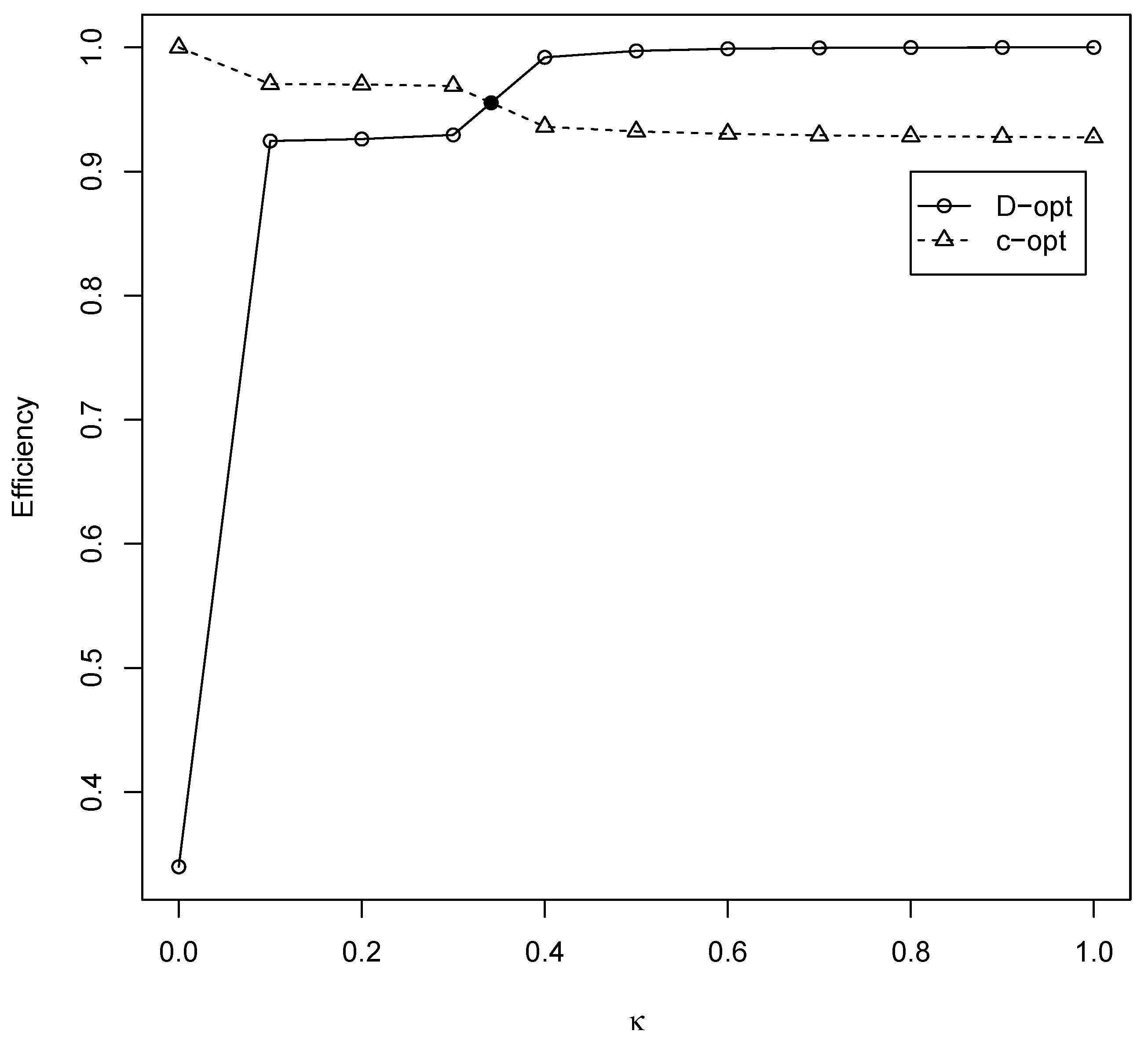
To obtain optimal PIC-I test plans that fulfill multiple design purposes, we compute -optimal compound designs for different weights , planning values , and removal proportions p. Some of the results are given in Table 3. The designs with and correspond to locally c- and D-optimal designs, respectively. From the table, we find that the optimal number of units remains constant, which is determined by the cost parameters, as we will discuss later. The results in Table 3 show us that -optimal designs depend on the planning values of , the weight , and the removal proportion p. With the increase of the removal proportion p, the number of inspections will decrease, but the length of the inspection interval will increase. The duration of the experiment will increase when the weight approaches 1. In addition, efficiencies of the -optimal designs with different to the locally D- and c-optimal designs imply that the -optimal designs can perform very well in most cases. However, in some special cases, such as and , the -optimal compound designs are very sensitive to the change of the weight parameter . Furthermore, with the increase of , the optimal number of inspections will increase or remain constant, and the duration for the design with is always larger than that of the design with . To choose a proper value of the weight , we suggest using the efficiency lines plot. Figure 1 gives an illustrating example where efficiencies of the -optimal compound designs for different to the locally D- and c-optimal designs are calculated and presented in a triangle or circle. Then, the horizontal coordinate of the intersection point of these two lines may be the best choice of .
In Table 4, we show -optimal PIC-I test plans for different weights and removal proportions when the sets of the planning values are and , respectively. Comparing the designs with and , we find that when the removal proportion increases, the number of inspections will decrease and the lengths of the inspection time intervals will increase. Designs with and indicate that when the uncertainty of the planning values increase, the numbers of inspections tend to increase or remain constant, the lengths of the inspection intervals tend to decrease, and the durations of the optimal designs will become longer for most cases. Furthermore, we also compute the efficiencies of the -optimal designs relative to the -optimal designs () and to the -optimal designs () by the formula given in (13), in which - and -optimality criteria are considered, respectively and then presented them in columns 8 (or 15) and 9 (or 16), respectively. By these efficiencies, the robust weights can be determined by the plot of efficiency lines, similar as we have shown in the -optimal compound designs.
5.3. Influence of the Cost Parameters
In order to investigate the influence of the cost parameters on the final robust optimal PIC-I test plans, we change the cost parameters over the sets , , , and compute the optimal test plans using Algorithm 1. The results for -optimal designs with are presented in Table 5. The ranges of the planning values are . It is observed from Table 5 that the number of units will increase with an increase of the budget C, but decrease with the increase of the cost of one test unit . The test plans are insensitive to the values of the cost parameter of one inspection . However, the number of inspections or the duration of the experiment will decrease or remain constant with the increase of the cost operation . Under different cost parameters, we also list the efficiencies of the -optimal designs to the locally optimal design with the planning values and . These efficiencies indicate that the performances of the robust -optimal designs are actually quite insensitive to the cost parameters.
5.4. Optimal General PIC-I Test Plans
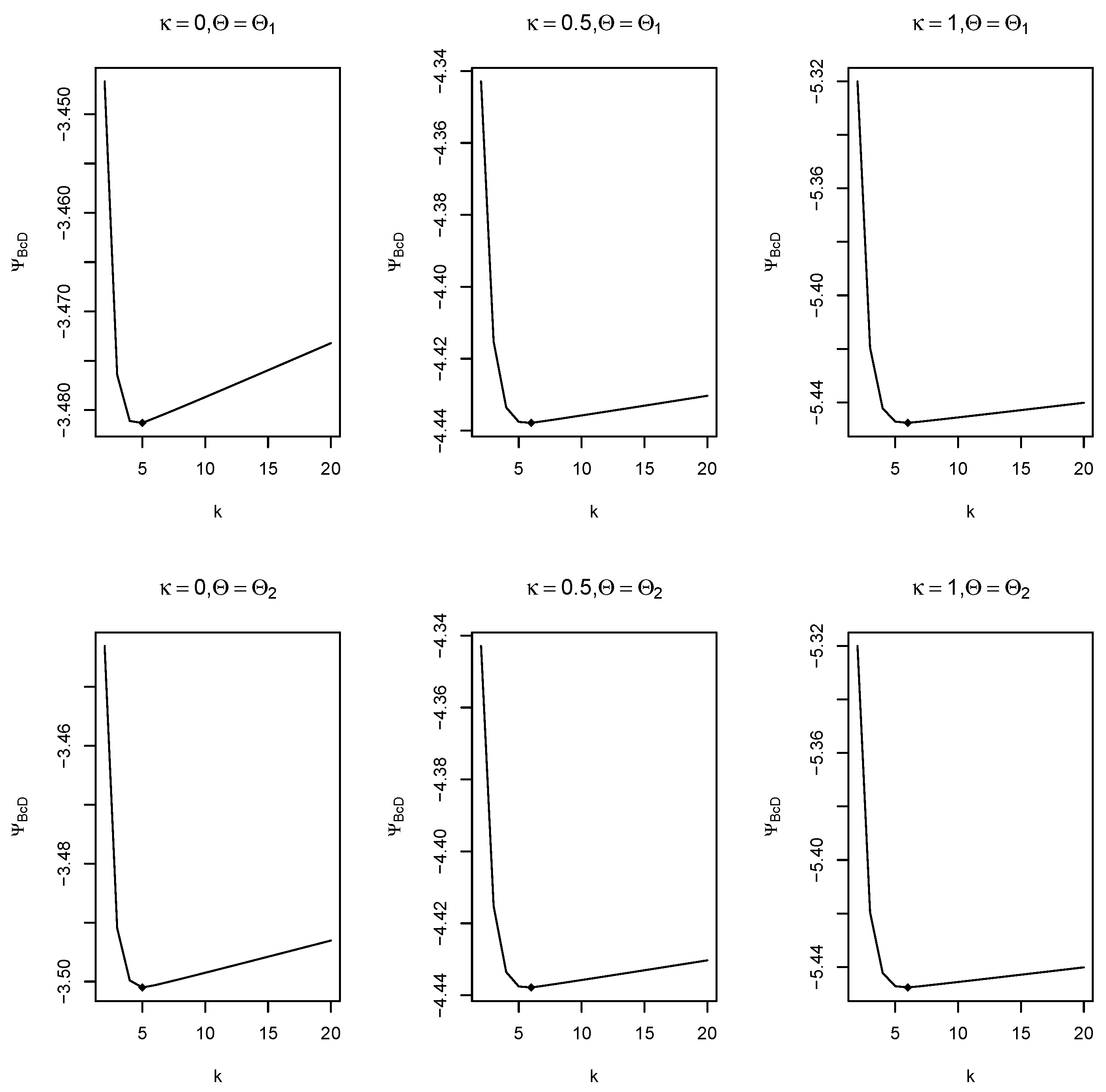
In this subsection, we consider the solution to the general problem given in (22). The model and values of the model parameters are the same as those described in the previous subsections. We use the PSO algorithm (Algorithm 2) to compute all general PIC-I test plans. Noting from the results in the previous tables that lengths of the inspection intervals are no more than 5, we then limit the lengths of the inspection intervals to the range of 0 to 10 in the PSO algorithm. The optimal PIC-I test plans are calculated for different design criteria and removal proportions. During the computation, we start Algorithm 2 by first setting , calculate the k-point optimal inspection time points and then the optimal size of test units N, and increase k by 1 until the optimality criterion function does not decrease or arrives at the maximum inspection time , see Algorithm 2 for details. We use the solutions obtained using the L-BFGS-B method as the initial values of the PSO algorithm. During the computation, we find that the design criterion is a convex function of k. See Figure 2 for an illustration. For the sake of saving space, we provide only the results with . Table 6 shows the locally D- and c-optimal PIC-I test plans for different number of inspections k and the values of their corresponding design criteria. Table 7 shows the -optimal PIC-I test plans with different when the regions of parameters are and , respectively. In Table 6 and Table 7, the optimal test plans are shown in bold. Looking at these tables we can see that the number of time points of every optimal PIC-I test plan does not exceed 10, which is very similar to its corresponding equispaced design. In Table 7, the efficiencies of k points -optimal designs relative to their corresponding locally ones given in Table 6 are also given in the last two columns. The results indicate that the -optimal test plans can perform very well in most situations, especially when the planning values are in the prior regions. Finally, to investigate the influence of the cost parameters on the optimal test plans, the -optimal designs are also calculated under different combinations of the cost parameters, and the results for are presented in Table 8. Similar conclusions to their corresponding ES designs can be drawn from the table.
| Algorithm 2 PSO Algorithm. |
|
6. A Real Life Example
In this section we consider a real data example, which contains 112 patients with plasma cell myeloma treated at the National Cancer Institute (Carbone et al. [37]) to illustrate our method. For easy reference, we reproduce this data set in Table 9. Note that this data set has been reanalysed by many authors (see Ng and Wang [6] and Lin and lio [8]) via different distributions and estimating methods (Balakrishnan and Cramer [2], Ch. 18). To be consistent with the topic we investigated in this paper, we fit the data by the Weibull distribution (1), similar as Ng and Wang [6], and the parameters are estimated by the maximum likelihood method. The resulted estimates are given as follows: and . Similar in the simulation example, we assume that the range of the values of and are and , respectively. Furthermore, we assume that the hyperparameters in the prior distributions and are . Since we have no any cost information for the original experiment, we then assume that /unit, , /m. Therefore, the total cost is . In - or -optimal design criteria, we set , which means that the median lifetime of survivors is of interest. In order to compare with the original inspection scheme , we first calculate the optimal ES and the general PIC-I test plans, respectively, assuming that the number of inspection times and the removal scheme are the same as in . The results for different design criteria are shown in Table 10 and Table 11, respectively. Efficiencies of under different design criteria are also given in the last column of these tables. These results indicate that the original inspection scheme has good robustness under different design criteria, except general D- and c-optimal design criteria. In addition, the optimal general PIC-I test plan has better performance than the corresponding ES test plan. Furthermore, considering different removal proportions, and , we redesign the Plasma cell myeloma inspection scheme. Optimal robust ES and general inspection schemes for different design criteria are shown in Table 12 and Table 13, respectively. The efficiencies of the original scheme are also listed in the last columns of these tables. These numerical results suggest that it is important to consider the removal proportions (or dropouts) at the design stage. The structures of robust PIC-I test schemes obtained under different design criteria may differ substantially.
7. Conclusions and Discussions
This paper considers robust optimal life testing plans under the PIC-I scheme. Based on the D-optimality and c-optimality, both the Bayesian and the minimax compound optimality criteria are proposed to obtain robust designs against the uncertainty of the model parameters and the design objectives. To make the designs more practical, the cost of the experiment at the design stage is taken into account. Two algorithms, including the MNO algorithm and the PSO algorithm, are proposed to solve the optimization problems. A numerical example and a real data example are provided to validate the feasibility and effectiveness of our methods. It is easy to see that the inspection times, the length of the inspection interval, and the experimental duration in the c- (- or -) optimal ES PIC-I test plan are less than the corresponding D- (- or -) optimal PIC-I test plan. Those in the - (- or -) optimal PIC-I test plan are somewhere in between. Increasing the removal proportion will reduce the number of the inspections and lengthen the inspection interval. With the increase of the uncertainty of the model parameters, the number of the inspections and the duration of the optimal PIC-I test plan tend to increase. The -optimal PIC-I test plan (not shown in the simulation example) tends to have more inspection times and longer duration of the experimental than its corresponding -optimal test plan. Similar conclusions can be drawn for the general optimal test plan. In addition, we should point out that the optimal PIC-I test plans depend on the budget of the experiment. We need to carefully set the larger coefficients in the cost function, because they will have a big impact on the experiment. Overall, our numerical results indicate that the proposed approaches can obtain better designs with improved robustness for conducting PIC-I life tests to estimate the model parameters and the qth quantile of the lifetime distribution efficiently. They also provide a coherent way to efficiently use one’s resources. Our approaches are intuitive and can be useful to engineers.
In this paper, to approximate the Bayesian and minimax design criteria, we choose finite percentiles of the prior parameter distributions. To improve the accuracy of these approximations, some Monte Carlo sampling methods and advanced optimization methods (Ruidas et al. [33]) need to be applied. This may be a topic worth studying in the future. This paper mainly focuses on obtaining robust designs under PIC-I test schemes when the model parameters are unknown and there are more than one design objective. However, there are still other uncertainties that need to be considered in the design stage. For example, many studies on designing PIC-I test plans assume that the lifetime data follow some symmetrical or asymmetrical distribution, such as Weibull (Wu et al. [14]), lognormal (Roy and Pradhan [17,19]), truncated normal (Lodhi and Tripathi [10]), and Exponentiated Frech’et (Wu and Chang [12]). In fact, many symmetric and asymmetric distributions have recently been proposed to fit lifetime data and evaluate the reliability of system (see [38,39,40,41]). When life time data is available, many methods of hypothesis testing have been provided to check the fitness of a given distribution (Jäntschi [42]). However, we need to point out that the life data is not available at the design stage, so the latent lifetime distribution may be uncertain. Therefore, it is an interesting topic to find robust designs against possible departures from underlying model assumptions (Zhao et al. [43]). In addition, our methods proposed in this paper can be extended to the situations of accelerated life test (Wu and Huang [44]) or degradation life test [45].
Author Contributions
Methodology, X.Z. and Y.W.; funding acquisition, R.Y.; software, X.Z. and Y.W.; writing, X.Z., Y.W. and R.Y. All authors have read and agreed to the published version of the manuscript.
Funding
This work was supported by the National Natural Science Foundation of China under Grants (11971318, 11871143) and Shanghai Rising-Star Program (No. 20QA1407500).
Institutional Review Board Statement
Not applicable.
Informed Consent Statement
Not applicable.
Data Availability Statement
The authors confirm that the data supporting the findings of this study are available within the article.
Acknowledgments
We express our sincere thanks to the editors and four reviewers for their insightful comments that have greatly improved this article.
Conflicts of Interest
The authors declare no conflict of interest.
References
- Balakrishnan, N.; Aggarwala, R. Progressive Censoring: Theory, Methods, and Applications; Birkhauser: Basel, Switzerland, 2000. [Google Scholar]
- Balakrishnan, N.; Cramer, E. The Art of Progressive Censoring; Birkhauser: New York, NY, USA, 2014. [Google Scholar]
- Balakrishnan, N. Progressive censoring methodology: An appraisal. Test 2007, 16, 211–259. [Google Scholar] [CrossRef]
- Aggarwala, R. Progressive interval censoring: Some mathematical results with applications to inference. Commun. Stat. Theory Methods 2001, 30, 1921–1935. [Google Scholar] [CrossRef]
- Xiang, L.; Tse, S.K. Maximum likelihood estimation in survival studies under progressive interval censoring with random removals. Biopharm. Stat. 2005, 15, 981–991. [Google Scholar] [CrossRef]
- Ng, H.K.T.; Wang, Z. Statistical estimation for the parameters of Weibull distribution based on progressively type I interval censored sample. J. Stat. Comput. Simul. 2009, 79, 145–159. [Google Scholar] [CrossRef]
- Chen, D.G.; Lio, Y.L. Parameter estimations for generalized exponential distribution under progressive type I interval censoring. Comput. Stat. Data. Anal. 2010, 54, 1581–1591. [Google Scholar] [CrossRef]
- Lin, Y.J.; Lio, Y.L. Bayesian inference under progressive type I interval censoring. J. Appl. Stat. 2012, 39, 1811–1824. [Google Scholar] [CrossRef]
- Singh, S.; Tripathi, Y.M. Estimating the parameters of an inverse Weibull distribution under progressive type I interval censoring. Stat. Pap. 2016, 59, 21–56. [Google Scholar] [CrossRef]
- Lodhi, C.; Tripathi, Y.M. Inference on a progressive type I interval-censored truncated normal distribution. J. Appl. Stat. 2020, 47, 1402–1422. [Google Scholar] [CrossRef]
- Budhiraja, S.; Pradhan, B. Point and interval estimation under progressive type-I interval censoring with random removal. Stat. Pap. 2020, 61, 445–477. [Google Scholar] [CrossRef]
- Wu, S.F.; Chang, W.T. The evaluation on the process capability index CL for exponentiated Frech—Et lifetime product under progressive type I interval censoring. Symmetry 2021, 13, 1032. [Google Scholar] [CrossRef]
- Alotaibi, R.; Rezk, H.; Dey, S.; Okasha, H. Bayesian estimation for Dagum distribution based on progressive type I interval censoring. PLoS ONE 2021, 16, e0252556. [Google Scholar] [CrossRef] [PubMed]
- Wu, S.J.; Chang, C.T.; Liao, K.J.; Huang, S.R. Planning of progressive group-censoring life tests with cost considerations. J. Appl. Stat. 2008, 35, 1293–1304. [Google Scholar] [CrossRef]
- Lin, C.T.; Wu, S.J.; Balakrishnan, N. Planning life tests with progressively type-I interval censored data from the lognormal distribution. J. Stat. Plan. Infer. 2009, 139, 54–61. [Google Scholar] [CrossRef]
- Lin, C.T.; Balakrishnan, N.; Wu, S.J. Planning life tests based on progressively type-I grouped censored data from the Weibull distribution. Comm. Statist. Simul. Comput. 2011, 40, 574–595. [Google Scholar] [CrossRef]
- Roy, S.; Pradhan, B. Bayesian optimum life testing plans under progressive type I interval censoring scheme. Quality Reliab. Eng. Int. 2017, 33, 2727–2737. [Google Scholar] [CrossRef]
- Budhiraja, S.; Pradhan, B. Optimum reliability acceptance sampling plans under progressive type-I interval censoring with random removal using a cost model. J. Appl. Stat. 2019, 46, 1492–1517. [Google Scholar] [CrossRef]
- Roy, S.; Pradhan, B. Bayesian C-optimal life testing plans under progressive type-I interval censoring scheme. Appl. Math. Model 2019, 70, 299–314. [Google Scholar] [CrossRef]
- Wu, S.F.; Liu, T.H.; Lai, Y.H.; Chang, W.T. A study on the experimental design for the lifetime performance index of rayleigh lifetime distribution under progressive type I interval censoring. Mathematics 2022, 10, 517. [Google Scholar] [CrossRef]
- Chaloner, K.; Verdinelli, I. Bayesian experimental design: A review. Statist. Sci. 1995, 10, 273–304. [Google Scholar] [CrossRef]
- Atkinson, A.C.; Donev, A.N.; Tobias, R.D. Optimum Experimental Designs with SAS; Oxford University Press: Oxford, UK, 2007. [Google Scholar]
- Yue, R.X.; Zhou, X.D. Robust integer-valued designs for linear random intercept models. Commun. Stat. Theory Methods 2018, 47, 4338–4354. [Google Scholar] [CrossRef]
- Pan, R.; Yang, T. Design and evaluation of accelerated life testing plans with dual objectives. J. Stat. Comput. Simul. 2014, 46, 114–126. [Google Scholar] [CrossRef]
- Bhattacharya, R.; Saha, B.N.; Farías, G.G.; Balakrishnan, N. Multi-criteria-based optimal life-testing plans under hybrid censoring scheme. TEST 2020, 29, 430–453. [Google Scholar] [CrossRef]
- Kundu, D. Bayesian inference and life testing plan for the Weibull distribution in presence of progressive censoring. Technometrics 2008, 50, 144–154. [Google Scholar] [CrossRef]
- Chernoff, H. Locally optimum designs for estimating parameters. Ann. Math. Statist. 1953, 24, 586–602. [Google Scholar] [CrossRef]
- Cook, R.D.; Wong, W.K. On the equivalence of constrained and compound designs. J. Am. Statist. Assoc. 1994, 89, 687–692. [Google Scholar] [CrossRef]
- Foo, L.K.; Duffull, S. Methods of robust design of nonlinear models with an application to pharmacokinetics. J. Biopharm. Stat. 2010, 20, 886–902. [Google Scholar] [CrossRef]
- Eberhart, R.; Kennedy, J. New optimizer using particle swarm theory. In Proceedings of the Sixth International Symposium on Micro Machine and Human Science, Nagoya, Japan, 4–6 October 1995; pp. 39–43. [Google Scholar]
- Poli, R.; Kennedy, J.; Blackwell, T. Particle swarm optimization an overview. Swarm. Intell. 2007, 1, 33–57. [Google Scholar] [CrossRef]
- Ruidas, S.; Seikh, M.R.; Nayak, P.K. A production inventory model with interval-valued carbon emission parameters under price-sensitive demand. Comput. Ind. Eng. 2021, 154, 107154. [Google Scholar] [CrossRef]
- Ruidas, S.; Seikh, M.R.; Nayak, P.K. Application of particle swarm optimization technique in an interval-valued EPQ model. In Meta-Heuristic Optimization Techniques: Applications in Engineering; Kumar, A., Pant, S., Ram, M., Yadav, O., Eds.; De Gruyter: Berlin, Germany; Boston, MA, USA, 2022; pp. 51–78. [Google Scholar]
- Chen, R.B.; Chen, P.Y.; Wong, W.K. Standardized maximin D optimal designs for pharmacological models via particle swarm optimization techniques. Chemom. Intell. Lab. Syst. 2018, 169, 79–86. [Google Scholar]
- Zhou, X.D.; Wang, Y.J.; Yue, R.X. Robust population designs for longitudinal linear regression model with a random intercept. Comput. Stat. 2018, 33, 903–931. [Google Scholar] [CrossRef]
- Liu, X.; Yue, R.X.; Zhang, Z.Z.; Wong, K.W. G-optimal designs for hierarchical linear models: An equivalence theorem and a nature-inspired meta-heuristic algorithm. Soft Comput. 2021, 25, 13549–13565. [Google Scholar] [CrossRef] [PubMed]
- Carbone, P.P.; Kellerhouse, L.E.; Gehan, E.A. Plasmacytic myeloma: A study of the relationship of survival to various clinical manifestations and anomalous protein type in 112 patients. Am. J. Med. 1967, 42, 937–948. [Google Scholar] [CrossRef]
- Chen, P.; Ye, Z.S. Approximate Statistical Limits for a Gamma Distribution. J. Qual. Technol. 2017, 49, 64–77. [Google Scholar] [CrossRef]
- Chen, P.; Ye, Z.S. Estimation of Field Reliability Based on Aggregate Lifetime Data. Technometrics 2017, 59, 115–125. [Google Scholar] [CrossRef]
- Xu, A.; Zhou, S.; Tang, Y. A unified model for system reliability evaluation under dynamic operating conditions. IEEE Trans. Reliab. 2020, 70, 65–72. [Google Scholar] [CrossRef]
- Luo, C.; Shen, L.; Xu, A. Modelling and estimation of system reliability under dynamic operating environments and lifetime ordering constraints. Reliab. Eng. Syst. Saf. 2022, 218, 108136. [Google Scholar] [CrossRef]
- Jäntschi, L. A test detecting the outliers for continuous distributions based on the cumulative distribution function of the data being tested. Symmetry 2019, 11, 835. [Google Scholar] [CrossRef] [Green Version]
- Zhao, X.J.; Pan, R.; del Castillo, E.; Xie, M. An adaptive two-stage Bayesian model averaging approach to planning and analyzing accelerated life tests under model uncertainty. J. Qual. Technol. 2019, 51, 181–197. [Google Scholar] [CrossRef]
- Wu, S.J.; Huang, S.R. Optimal progressive interval censoring plan under accelerated life test with limited budget. J. Stat. Comput. Simul. 2019, 89, 3241–3257. [Google Scholar] [CrossRef]
- Hu, J.; Chen, P. Predictive maintenance of systems subject to hard failure based on proportional hazards model. Reliab. Eng. Syst. Saf. 2020, 196, 106707. [Google Scholar] [CrossRef]
Figure 1.
Efficiency lines of -optimal compound designs for different weights when the planning values are and the removal proportion is .
Figure 1.
Efficiency lines of -optimal compound designs for different weights when the planning values are and the removal proportion is .

Figure 2.
Plots of with k inspection time points and for different weights and parameters space .


Table 1.
Locally optimal PIC-I test plans for different removal proportions p, planning values of , and design criteria.
Table 1.
Locally optimal PIC-I test plans for different removal proportions p, planning values of , and design criteria.
| p | D-Optimality | c-Optimality | ||||||||||||
|---|---|---|---|---|---|---|---|---|---|---|---|---|---|---|
| 0.1 | 74 | 6 | 2.0121 | 12.0724 | −6.1284 | 0.9079 | 74 | 4 | 1.9860 | 7.9439 | −4.0028 | 0.9975 | ||
| 0.1 | 74 | 9 | 2.1483 | 19.3346 | −5.1970 | 0.9272 | 74 | 6 | 1.7824 | 10.6944 | −3.1115 | 0.9882 | ||
| 0.1 | 74 | 6 | 2.6201 | 15.7203 | −6.1268 | 0.9076 | 74 | 4 | 2.5874 | 10.3497 | −4.0018 | 0.9970 | ||
| 0.1 | 73 | 9 | 2.7913 | 25.1220 | −5.1945 | 0.8753 | 74 | 5 | 2.4145 | 12.0724 | −3.1102 | 0.9873 | ||
| 0.3 | 74 | 4 | 3.0280 | 12.1120 | −5.8608 | 0.9886 | 74 | 3 | 3.0755 | 9.2264 | −3.8758 | 0.9981 | ||
| 0.3 | 74 | 6 | 3.1140 | 18.6839 | −4.9051 | 0.9493 | 74 | 4 | 2.6947 | 10.7789 | −3.0115 | 0.9835 | ||
| 0.3 | 74 | 4 | 3.9453 | 15.7813 | −5.8592 | 0.9888 | 74 | 3 | 4.0074 | 12.0222 | −3.8746 | 0.9977 | ||
| 0.3 | 74 | 6 | 4.0537 | 24.3223 | −4.9027 | 0.9499 | 74 | 4 | 3.5113 | 14.0454 | −3.0101 | 0.9828 | ||
| 0.1 | 74 | 6 | 1.4656 | 8.7933 | −6.7534 | 0.9369 | 74 | 4 | 1.5798 | 6.3191 | −4.6350 | 0.9969 | ||
| 0.1 | 73 | 11 | 1.8835 | 20.7189 | −4.8260 | 0.8784 | 74 | 6 | 1.4889 | 8.9334 | −2.7718 | 0.9797 | ||
| 0.1 | 74 | 6 | 2.4859 | 14.9152 | −6.7508 | 0.9361 | 74 | 4 | 2.6829 | 10.7315 | −4.6332 | 0.9961 | ||
| 0.1 | 73 | 10 | 3.2318 | 32.3185 | −4.8203 | 0.8794 | 74 | 6 | 2.5223 | 15.1340 | −2.7691 | 0.9770 | ||
| 0.3 | 74 | 3 | 3.1648 | 9.4943 | −6.4923 | 0.3398 | 74 | 2 | 4.2754 | 8.5508 | −4.4716 | 0.9275 | ||
| 0.3 | 74 | 7 | 2.7790 | 19.4529 | −4.5149 | 0.9059 | 74 | 4 | 2.2228 | 8.8912 | −2.6749 | 0.9630 | ||
| 0.3 | 74 | 2 | 5.4124 | 10.8248 | −6.4900 | 0.3398 | 74 | 2 | 7.2750 | 14.5501 | −4.4691 | 0.9287 | ||
| 0.3 | 73 | 6 | 4.7729 | 28.6373 | −4.5095 | 0.9078 | 74 | 4 | 3.7753 | 15.1014 | −2.6723 | 0.9595 | ||
Table 2.
Progressively type-I interval-censored samples.
| i | 1 | 2 | 3 | 4 | 5 |
|---|---|---|---|---|---|
| 2 | 4 | 6 | 2 | 1 | |
| 0 | 2 | 1 | 1 | 1 | |
| 0 | 0.2 | 0.3 | 0.4 | 1 |
Table 3.
-optimal PIC-I test plans for different weights , different removal proportions p, and the different planning values .
Table 3.
-optimal PIC-I test plans for different weights , different removal proportions p, and the different planning values .
| p | |||||||||||||||
|---|---|---|---|---|---|---|---|---|---|---|---|---|---|---|---|
| 0.1 | 0.0 | 74 | 5 | 1.7235 | 8.6174 | −3.5486 | 0.9359 | 1.0000 | 74 | 4 | 1.5798 | 6.3191 | −4.6350 | 0.9369 | 1.0000 |
| 0.1 | 74 | 7 | 1.7453 | 12.2173 | −3.7574 | 0.9961 | 0.9976 | 74 | 5 | 1.5582 | 7.7908 | −4.8458 | 0.9981 | 0.9990 | |
| 0.2 | 74 | 7 | 1.7762 | 12.4334 | −3.9686 | 0.9974 | 0.9973 | 74 | 5 | 1.5587 | 7.7933 | −5.0575 | 0.9981 | 0.9990 | |
| 0.3 | 74 | 7 | 1.8025 | 12.6172 | −4.1800 | 0.9983 | 0.9971 | 74 | 5 | 1.5590 | 7.7951 | −5.2693 | 0.9981 | 0.9990 | |
| 0.4 | 74 | 7 | 1.8254 | 12.7781 | −4.3915 | 0.9989 | 0.9967 | 74 | 5 | 1.5593 | 7.7964 | −5.4810 | 0.9981 | 0.9990 | |
| 0.5 | 74 | 7 | 1.8460 | 12.9219 | −4.6031 | 0.9993 | 0.9964 | 74 | 6 | 1.5021 | 9.0127 | −5.6929 | 0.9998 | 0.9975 | |
| 0.6 | 74 | 7 | 1.8646 | 13.0523 | −4.8148 | 0.9996 | 0.9960 | 74 | 6 | 1.4936 | 8.9619 | −5.9049 | 0.9999 | 0.9974 | |
| 0.7 | 74 | 7 | 1.8817 | 13.1720 | −5.0265 | 0.9998 | 0.9957 | 74 | 6 | 1.4858 | 8.9146 | −6.1170 | 0.9999 | 0.9973 | |
| 0.8 | 74 | 7 | 1.8975 | 13.2828 | −5.2383 | 0.9999 | 0.9953 | 74 | 6 | 1.4785 | 8.8709 | −6.3291 | 1.0000 | 0.9972 | |
| 0.9 | 74 | 7 | 1.9123 | 13.3858 | −5.4501 | 1.0000 | 0.9949 | 74 | 6 | 1.4717 | 8.8305 | −6.5413 | 1.0000 | 0.9970 | |
| 1.0 | 74 | 7 | 1.9261 | 13.4827 | −5.6620 | 1.0000 | 0.9946 | 74 | 6 | 1.4656 | 8.7935 | −6.7534 | 1.0000 | 0.9969 | |
| 0.3 | 0.0 | 74 | 3 | 2.6524 | 7.9573 | −3.4414 | 0.9312 | 1.0000 | 74 | 2 | 4.2754 | 8.5508 | −4.4716 | 0.3398 | 1.0000 |
| 0.1 | 74 | 4 | 2.6559 | 10.6235 | −3.6342 | 0.9932 | 0.9986 | 74 | 3 | 2.5149 | 7.5447 | −4.6388 | 0.9246 | 0.9704 | |
| 0.2 | 74 | 4 | 2.6845 | 10.7380 | −3.8285 | 0.9945 | 0.9984 | 74 | 3 | 2.4851 | 7.4553 | −4.8361 | 0.9262 | 0.9701 | |
| 0.3 | 74 | 5 | 2.6693 | 13.3467 | −4.0233 | 0.9992 | 0.9969 | 74 | 3 | 2.4346 | 7.3038 | −5.0338 | 0.9295 | 0.9689 | |
| 0.4 | 74 | 5 | 2.6839 | 13.4197 | −4.2183 | 0.9994 | 0.9968 | 74 | 3 | 3.0484 | 9.1453 | −5.2371 | 0.9920 | 0.9361 | |
| 0.5 | 74 | 5 | 2.6982 | 13.4909 | −4.4134 | 0.9996 | 0.9967 | 74 | 3 | 3.0973 | 9.2918 | −5.4455 | 0.9972 | 0.9323 | |
| 0.6 | 74 | 5 | 2.7121 | 13.5604 | −4.6084 | 0.9998 | 0.9965 | 74 | 3 | 3.1230 | 9.3690 | −5.6545 | 0.9989 | 0.9304 | |
| 0.7 | 74 | 5 | 2.7257 | 13.6285 | −4.8036 | 0.9999 | 0.9963 | 74 | 3 | 3.1392 | 9.4175 | −5.8638 | 0.9996 | 0.9292 | |
| 0.8 | 74 | 5 | 2.7390 | 13.6950 | −4.9987 | 0.9999 | 0.9960 | 74 | 3 | 3.1503 | 9.4510 | −6.0732 | 0.9999 | 0.9284 | |
| 0.9 | 74 | 5 | 2.7520 | 13.7600 | −5.1939 | 1.0000 | 0.9958 | 74 | 3 | 3.1585 | 9.4755 | −6.2827 | 1.0000 | 0.9279 | |
| 1.0 | 74 | 5 | 2.7648 | 13.8238 | −5.3891 | 1.0000 | 0.9955 | 74 | 3 | 3.1648 | 9.4943 | −6.4923 | 1.0000 | 0.9275 | |
Table 4.
-optimal PIC-I test plans for different weights and different removal proportions p when the sets of the planning values are and , respectively.
Table 4.
-optimal PIC-I test plans for different weights and different removal proportions p when the sets of the planning values are and , respectively.
| p | |||||||||||||||
|---|---|---|---|---|---|---|---|---|---|---|---|---|---|---|---|
| 0.1 | 0.0 | 74 | 5 | 2.1731 | 10.8654 | −3.5759 | 0.9360 | 1.0000 | 74 | 6 | 2.0791 | 12.4747 | −3.6117 | 0.9673 | 1.0000 |
| 0.1 | 74 | 7 | 2.1752 | 15.2266 | −3.7842 | 0.9942 | 0.9977 | 74 | 7 | 2.1093 | 14.7654 | −3.8200 | 0.9894 | 0.9989 | |
| 0.2 | 74 | 7 | 2.2187 | 15.5306 | −3.9950 | 0.9959 | 0.9974 | 74 | 8 | 2.1187 | 16.9493 | −4.0297 | 0.9966 | 0.9976 | |
| 0.3 | 74 | 7 | 2.2559 | 15.7910 | −4.2059 | 0.9970 | 0.9970 | 74 | 8 | 2.1503 | 17.2027 | −4.2399 | 0.9975 | 0.9973 | |
| 0.4 | 74 | 7 | 2.2885 | 16.0192 | −4.4169 | 0.9978 | 0.9966 | 74 | 8 | 2.1789 | 17.4312 | −4.4503 | 0.9981 | 0.9969 | |
| 0.5 | 74 | 8 | 2.2654 | 18.1234 | −4.6283 | 0.9994 | 0.9955 | 74 | 8 | 2.2048 | 17.6381 | −4.6607 | 0.9986 | 0.9965 | |
| 0.6 | 74 | 8 | 2.2880 | 18.3039 | −4.8397 | 0.9996 | 0.9952 | 74 | 9 | 2.1921 | 19.7287 | −4.8714 | 0.9996 | 0.9953 | |
| 0.7 | 74 | 8 | 2.3091 | 18.4726 | −5.0511 | 0.9998 | 0.9949 | 74 | 9 | 2.2116 | 19.9047 | −5.0821 | 0.9998 | 0.9950 | |
| 0.8 | 74 | 8 | 2.3289 | 18.6311 | −5.2626 | 0.9999 | 0.9945 | 74 | 9 | 2.2299 | 20.0691 | −5.2929 | 0.9999 | 0.9947 | |
| 0.9 | 74 | 8 | 2.3476 | 18.7806 | −5.4742 | 1.0000 | 0.9942 | 74 | 9 | 2.2470 | 20.2229 | −5.5038 | 1.0000 | 0.9944 | |
| 1.0 | 74 | 8 | 2.3653 | 18.9221 | −5.6858 | 1.0000 | 0.9938 | 74 | 9 | 2.2630 | 20.3672 | −5.7146 | 1.0000 | 0.9941 | |
| 0.3 | 0.0 | 74 | 3 | 3.3461 | 10.0384 | −3.4621 | 0.9323 | 1.0000 | 74 | 4 | 3.1924 | 12.7695 | −3.4840 | 0.9817 | 1.0000 |
| 0.1 | 74 | 4 | 3.3257 | 13.3029 | −3.6553 | 0.9906 | 0.9994 | 74 | 5 | 3.2009 | 16.0044 | −3.6769 | 0.9960 | 0.9987 | |
| 0.2 | 74 | 5 | 3.3230 | 16.6148 | −3.8494 | 0.9986 | 0.9976 | 74 | 5 | 3.2300 | 16.1501 | −3.8712 | 0.9969 | 0.9986 | |
| 0.3 | 74 | 5 | 3.3438 | 16.7190 | −4.0442 | 0.9990 | 0.9974 | 74 | 5 | 3.2584 | 16.2922 | −4.0656 | 0.9976 | 0.9983 | |
| 0.4 | 74 | 5 | 3.3641 | 16.8204 | −4.2392 | 0.9993 | 0.9973 | 74 | 5 | 3.2860 | 16.4299 | −4.2601 | 0.9982 | 0.9980 | |
| 0.5 | 74 | 5 | 3.3838 | 16.9191 | −4.4341 | 0.9995 | 0.9971 | 74 | 5 | 3.3126 | 16.5628 | −4.4547 | 0.9987 | 0.9976 | |
| 0.6 | 74 | 5 | 3.4031 | 17.0154 | −4.6291 | 0.9997 | 0.9969 | 74 | 5 | 3.3381 | 16.6903 | −4.6494 | 0.9990 | 0.9972 | |
| 0.7 | 74 | 5 | 3.4219 | 17.1094 | −4.8242 | 0.9998 | 0.9966 | 74 | 5 | 3.3624 | 16.8121 | −4.8441 | 0.9993 | 0.9967 | |
| 0.8 | 74 | 5 | 3.4403 | 17.2013 | −5.0193 | 0.9999 | 0.9963 | 74 | 6 | 3.3533 | 20.1196 | −5.0391 | 0.9999 | 0.9950 | |
| 0.9 | 74 | 5 | 3.4582 | 17.2911 | −5.2144 | 1.0000 | 0.9960 | 74 | 6 | 3.3739 | 20.2431 | −5.2341 | 1.0000 | 0.9946 | |
| 1.0 | 74 | 5 | 3.4758 | 17.3789 | −5.4096 | 1.0000 | 0.9957 | 74 | 6 | 3.3936 | 20.3614 | −5.4292 | 1.0000 | 0.9941 | |
Table 5.
-optimal PIC-I test plans for different cost parameters and weight parameters / when the removal proportion is and .
Table 5.
-optimal PIC-I test plans for different cost parameters and weight parameters / when the removal proportion is and .
| C | N | k | |||||||||
|---|---|---|---|---|---|---|---|---|---|---|---|
| 0 | 4000 | 80 | 3 | 2.5 | 49 | 3 | 3.3415 | 10.0244 | −3.0538 | 0.9924 | 0.9962 |
| 6000 | 74 | 3 | 3.3461 | 10.0384 | −3.4621 | 0.9917 | 0.9963 | ||||
| 8000 | 99 | 3 | 3.3485 | 10.0454 | −3.7512 | 0.9913 | 0.9963 | ||||
| 6000 | 70 | 3 | 2.5 | 85 | 3 | 3.3461 | 10.0384 | −3.5956 | 0.9917 | 0.9963 | |
| 80 | 74 | 3 | 3.3461 | 10.0384 | −3.4621 | 0.9917 | 0.9963 | ||||
| 90 | 66 | 3 | 3.3461 | 10.0384 | −3.3443 | 0.9917 | 0.9963 | ||||
| 6000 | 80 | 2 | 2.5 | 74 | 3 | 3.3461 | 10.0384 | −3.4626 | 0.9915 | 0.9963 | |
| 3 | 74 | 3 | 3.3461 | 10.0384 | −3.4621 | 0.9917 | 0.9963 | ||||
| 5 | 74 | 3 | 3.3461 | 10.0384 | −3.4611 | 0.9920 | 0.9963 | ||||
| 6000 | 80 | 3 | 1.0 | 74 | 4 | 3.2950 | 13.1801 | −3.4649 | 0.9956 | 0.9966 | |
| 2.5 | 74 | 3 | 3.3461 | 10.0384 | −3.4621 | 0.9917 | 0.9963 | ||||
| 4.0 | 74 | 3 | 3.3405 | 10.0216 | −3.4596 | 0.9923 | 0.9962 | ||||
| 0.5 | 4000 | 80 | 3 | 2.5 | 49 | 5 | 3.3742 | 16.8709 | −4.0238 | 0.9892 | 0.9896 |
| 6000 | 74 | 5 | 3.3838 | 16.9191 | −4.4341 | 0.9900 | 0.9914 | ||||
| 8000 | 99 | 5 | 3.3886 | 16.9432 | −4.7242 | 0.9904 | 0.9923 | ||||
| 6000 | 70 | 3 | 2.5 | 84 | 5 | 3.3838 | 16.9191 | −4.5677 | 0.9900 | 0.9914 | |
| 80 | 74 | 5 | 3.3838 | 16.9191 | −4.4341 | 0.9900 | 0.9914 | ||||
| 90 | 66 | 5 | 3.3838 | 16.9191 | −4.3164 | 0.9900 | 0.9914 | ||||
| 6000 | 80 | 2 | 2.5 | 74 | 5 | 3.3838 | 16.9192 | −4.4350 | 0.9902 | 0.9917 | |
| 3 | 74 | 5 | 3.3838 | 16.9191 | −4.4341 | 0.9900 | 0.9914 | ||||
| 5 | 74 | 5 | 3.3838 | 16.9190 | −4.4325 | 0.9897 | 0.9907 | ||||
| 6000 | 80 | 3 | 1.0 | 74 | 5 | 3.3953 | 16.9767 | −4.4384 | 0.9907 | 0.9930 | |
| 2.5 | 74 | 5 | 3.3838 | 16.9191 | −4.4341 | 0.9900 | 0.9914 | ||||
| 4.0 | 73 | 5 | 3.3723 | 16.8615 | −4.4299 | 0.9893 | 0.9898 | ||||
| 1 | 4000 | 80 | 3 | 2.5 | 49 | 5 | 3.4664 | 17.3321 | −4.9992 | 0.9847 | 0.9864 |
| 6000 | 74 | 5 | 3.4758 | 17.3789 | −5.4096 | 0.9856 | 0.9883 | ||||
| 8000 | 99 | 5 | 3.4805 | 17.4023 | −5.6997 | 0.9860 | 0.9892 | ||||
| 6000 | 70 | 3 | 2.5 | 84 | 5 | 3.4758 | 17.3789 | −5.5431 | 0.9856 | 0.9883 | |
| 80 | 74 | 5 | 3.4758 | 17.3789 | −5.4096 | 0.9856 | 0.9883 | ||||
| 90 | 66 | 5 | 3.4758 | 17.3789 | −5.2918 | 0.9856 | 0.9883 | ||||
| 6000 | 80 | 2 | 2.5 | 74 | 5 | 3.4758 | 17.3790 | −5.4104 | 0.9858 | 0.9886 | |
| 3 | 74 | 5 | 3.4758 | 17.3789 | −5.4096 | 0.9856 | 0.9883 | ||||
| 5 | 74 | 5 | 3.4758 | 17.3788 | −5.4079 | 0.9853 | 0.9876 | ||||
| 6000 | 80 | 3 | 1.0 | 74 | 5 | 3.4870 | 17.4348 | −5.4140 | 0.9863 | 0.9899 | |
| 2.5 | 74 | 5 | 3.4758 | 17.3789 | −5.4096 | 0.9856 | 0.9883 | ||||
| 4.0 | 73 | 5 | 3.4646 | 17.3229 | −5.4052 | 0.9849 | 0.9867 |
Table 6.
Locally D- and c-optimal general PIC-I test plans for different numbers of inspections with , and .
Table 6.
Locally D- and c-optimal general PIC-I test plans for different numbers of inspections with , and .
| k | N | Inspection Times | ||
|---|---|---|---|---|
| 2 | 74 | (2.612, 8.067) | −5.3216 | |
| 3 | 74 | (2.547, 7.214, 9.929) | −5.4120 | |
| D-opt | 4 | 74 | (2.521, 6.961, 9.235, 11.333) | −5.4308 |
| 5 | 74 | (2.514, 6.896, 9.066, 10.767, 12.455) | −5.4344 | |
| 6 | 74 | (2.512, 6.881, 9.029, 10.644, 12.002, 13.207) | −5.4346 | |
| 7 | 74 | (2.512, 6.879, 9.025, 10.629, 11.948, 12.999, 13.434) | −5.4341 | |
| 2 | 74 | (3.154, 5.554) | −3.4366 | |
| c-opt | 3 | 74 | (2.970, 4.886, 6.724) | −3.4581 |
| 4 | 74 | (2.934, 4.761, 6.216, 7.603) | −3.4610 | |
| 5 | 74 | (2.928, 4.741, 6.140, 7.252, 8.083) | −3.4609 |
Table 7.
-optimal general PIC-I test plans for different numbers of inspections with and .
| k | N | Inspection Times | |||||
|---|---|---|---|---|---|---|---|
| 0 | 2 | 74 | (3.911, 7.256) | −3.4467 | 0.8388 | 0.8882 | |
| 3 | 74 | (3.700, 6.219, 8.875) | −3.4764 | 0.8693 | 0.9238 | ||
| 4 | 74 | (3.658, 6.020, 8.051, 10.269) | −3.4811 | 0.8791 | 0.9314 | ||
| 5 | 74 | (3.650, 5.983, 7.900, 9.628, 11.190) | −3.4813 | 0.8818 | 0.9329 | ||
| 6 | 74 | (3.650, 5.982, 7.892, 9.595, 11.047, 11.312) | −3.4808 | 0.8816 | 0.9329 | ||
| 0.5 | 2 | 74 | (3.811, 9.328) | −4.3429 | 0.8983 | 0.8882 | |
| 3 | 74 | (3.540, 7.755, 11.515) | −4.4152 | 0.9313 | 0.9088 | ||
| 4 | 74 | (3.453, 7.255, 10.413, 13.462) | −4.4335 | 0.9383 | 0.9218 | ||
| 5 | 74 | (3.430, 7.122, 10.123, 12.563, 15.151) | −4.4376 | 0.9407 | 0.9256 | ||
| 6 | 74 | (3.424, 7.090, 10.053, 12.353, 14.409, 16.276) | −4.4378 | 0.9414 | 0.9263 | ||
| 7 | 74 | (3.423, 7.087, 10.046, 12.334, 14.342, 16.028, 16.511) | −4.4373 | 0.9415 | 0.9263 | ||
| 1 | 2 | 74 | (3.304, 9.810) | −5.3200 | 0.8949 | 0.8700 | |
| 3 | 74 | (3.227, 8.798, 12.277) | −5.4196 | 0.9254 | 0.8763 | ||
| 4 | 74 | (3.193, 8.480, 11.343, 14.299) | −5.4422 | 0.9367 | 0.8813 | ||
| 5 | 74 | (3.183, 8.389, 11.098, 13.437, 16.036) | −5.4472 | 0.9405 | 0.8829 | ||
| 6 | 74 | (3.180, 8.366, 11.037, 13.234, 15.279, 17.240) | −5.4476 | 0.9414 | 0.8831 | ||
| 7 | 74 | (3.180, 8.363, 11.030, 13.209, 15.188, 16.899, 17.583) | −5.4472 | 0.9415 | 0.8831 | ||
| 0 | 2 | 74 | (3.835, 7.571) | −3.4431 | 0.8794 | 0.8994 | |
| 3 | 74 | (3.590, 6.233, 9.451) | −3.4909 | 0.8914 | 0.9388 | ||
| 4 | 74 | (3.538, 5.963, 8.319, 11.210) | −3.4998 | 0.8963 | 0.9472 | ||
| 5 | 74 | (3.527, 5.902, 8.074, 10.268, 12.605) | −3.5010 | 0.8986 | 0.9490 | ||
| 6 | 74 | (3.525 5.892 8.035 10.126 12.055 13.172) | −3.5006 | 0.8993 | 0.9492 | ||
| 0.5 | 2 | 74 | (3.713, 8.514) | −4.3305 | 0.9316 | 0.9037 | |
| 3 | 74 | (3.469, 7.312, 11.248) | −4.4273 | 0.9320 | 0.9233 | ||
| 4 | 74 | (3.389, 6.910, 10.013, 13.540) | −4.4508 | 0.9390 | 0.9341 | ||
| 5 | 74 | (3.364, 6.784, 9.666, 12.385, 15.614) | −4.4566 | 0.9424 | 0.9377 | ||
| 6 | 74 | (3.357, 6.750, 9.572, 12.096, 14.599, 17.120) | −4.4573 | 0.9435 | 0.9384 | ||
| 7 | 74 | (3.356,6.745,9.559,12.055,14.459,16.629,17.601) | −4.4569 | 0.9436 | 0.9384 | ||
| 1 | 2 | 74 | (3.235, 8.905) | −5.2680 | 0.9631 | 0.8940 | |
| 3 | 74 | (3.157, 7.951, 11.858) | −5.4075 | 0.9569 | 0.9023 | ||
| 4 | 74 | (3.120, 7.644, 10.724, 14.294) | −5.4409 | 0.9634 | 0.9082 | ||
| 5 | 74 | (3.106, 7.544, 10.403, 13.144, 16.511) | −5.4492 | 0.9667 | 0.9103 | ||
| 6 | 74 | (3.101, 7.515, 10.315, 12.851, 15.443, 18.249) | −5.4506 | 0.9677 | 0.9106 | ||
| 7 | 74 | (3.101, 7.510, 10.298, 12.796, 15.253, 17.559, 19.001) | −5.4503 | 0.9679 | 0.9105 |
Table 8.
-optimal general PIC-I test plans for different cost parameters and weight parameters when the removal proportion and .
Table 8.
-optimal general PIC-I test plans for different cost parameters and weight parameters when the removal proportion and .
| C | N | Inspection Times | |||||
|---|---|---|---|---|---|---|---|
| 4000 | 80 | 3 | 2.5 | 49 | (3.659, 6.020, 8.035, 10.159) | −3.0725 | |
| 6000 | 74 | (3.650, 5.983, 7.900, 9.628, 11.190) | −3.4813 | ||||
| 8000 | 99 | (3.650, 5.982, 7.902, 9.658, 11.371) | −3.7708 | ||||
| 6000 | 70 | 3 | 2.5 | 85 | (3.650, 5.983, 7.900, 9.628, 11.190) | −3.6148 | |
| 80 | 74 | (3.650, 5.983, 7.900, 9.628, 11.190) | −3.4813 | ||||
| 0 | 90 | 66 | (3.650, 5.983, 7.900, 9.628, 11.190) | −3.3635 | |||
| 6000 | 80 | 2 | 2.5 | 74 | (3.650, 5.983, 7.900, 9.628, 11.190) | −3.4821 | |
| 3 | 74 | (3.650, 5.983, 7.900, 9.628, 11.190) | −3.4813 | ||||
| 5 | 74 | (3.658, 6.020, 8.051, 10.269) | −3.4798 | ||||
| 6000 | 80 | 3 | 1.0 | 74 | (3.649, 5.981, 7.908, 9.712, 11.677) | −3.4842 | |
| 2.5 | 74 | (3.650, 5.983, 7.900, 9.628, 11.190) | −3.4813 | ||||
| 4.0 | 74 | (3.659, 6.020, 8.032, 10.138) | −3.4785 | ||||
| 4000 | 80 | 3 | 2.5 | 49 | (3.428, 7.115, 10.106, 12.509, 14.948) | −4.0277 | |
| 6000 | 74 | (3.424, 7.090, 10.053, 12.353, 14.409, 16.276) | −4.4378 | ||||
| 8000 | 99 | (3.425, 7.092, 10.058, 12.372, 14.478, 16.538) | −4.7280 | ||||
| 6000 | 70 | 3 | 2.5 | 84 | (3.424, 7.090, 10.053, 12.353, 14.409, 16.276) | −4.5714 | |
| 80 | 74 | (3.424, 7.090, 10.053, 12.353, 14.409, 16.276) | −4.4378 | ||||
| 0.5 | 90 | 66 | (3.424, 7.090, 10.053, 12.353, 14.409, 16.276) | −4.3200 | |||
| 6000 | 80 | 2 | 2.5 | 74 | (3.424, 7.090, 10.053, 12.353, 14.409, 16.277) | −4.4388 | |
| 3 | 74 | (3.424, 7.090, 10.053, 12.353, 14.409, 16.276) | −4.4378 | ||||
| 5 | 74 | (3.430, 7.122, 10.123, 12.562, 15.151) | −4.4359 | ||||
| 6000 | 80 | 3 | 1.0 | 74 | (3.426, 7.096, 10.068, 12.403, 14.592, 16.976) | −4.4420 | |
| 2.5 | 74 | (3.424, 7.090, 10.053, 12.353, 14.409, 16.276) | −4.4378 | ||||
| 4.0 | 73 | (3.422, 7.085, 10.042, 12.316, 14.271, 15.755) | −4.4338 | ||||
| 4000 | 80 | 3 | 2.5 | 49 | (3.182, 8.384, 11.085, 13.392, 15.858) | −5.0371 | |
| 6000 | 74 | (3.180, 8.366, 11.037, 13.234, 15.279, 17.240) | −5.4476 | ||||
| 8000 | 99 | (3.181, 8.367, 11.042, 13.250, 15.341, 17.480) | −5.7379 | ||||
| 6000 | 70 | 3 | 2.5 | 84 | (3.180, 8.366, 11.037, 13.234, 15.279, 17.240) | −5.5812 | |
| 80 | 74 | (3.180, 8.366, 11.037, 13.234, 15.279, 17.240) | −5.4476 | ||||
| 90 | 65 | (3.180, 8.366, 11.037, 13.234, 15.279, 17.240) | −5.3299 | ||||
| 1 | 6000 | 80 | 2 | 2.5 | 74 | (3.180, 8.366, 11.037, 13.234, 15.279, 17.241) | −5.4487 |
| 3 | 74 | (3.180, 8.366, 11.037, 13.234, 15.279, 17.240) | −5.4476 | ||||
| 5 | 74 | (3.180, 8.366, 11.037, 13.234, 15.279, 17.238) | −5.4456 | ||||
| 6000 | 80 | 3 | 1.0 | 74 | (3.181, 8.370, 11.049, 13.277, 15.442, 17.875) | −5.4521 | |
| 2.5 | 74 | (3.180, 8.366, 11.037, 13.234, 15.279, 17.240) | −5.4476 | ||||
| 4.0 | 73 | (3.179, 8.363, 11.028, 13.201, 15.153, 16.760) | −5.4433 |
Table 9.
Plasma cell myeloma survival times.
| Interval in Months | Number at Risk | Number of Withdrawals |
|---|---|---|
| 112 | 1 | |
| 93 | 1 | |
| 76 | 3 | |
| 55 | 0 | |
| 45 | 0 | |
| 34 | 1 | |
| 25 | 2 | |
| 10 | 3 | |
| 3 | 2 | |
| 0 | 0 |
Table 10.
Optimal ES PIC-I test plans in the real data example when the removal scheme is the same as that in the original design.
Table 10.
Optimal ES PIC-I test plans in the real data example when the removal scheme is the same as that in the original design.
| Design Criterion | N | |||||
|---|---|---|---|---|---|---|
| D-opt | - | 132 | 3.5972 | 32.3744 | −9.6813 | 0.8243 |
| c-opt | - | 134 | 3.1923 | 28.7311 | −9.6071 | 0.8233 |
| BcD-opt | 0.0 | 128 | 4.8029 | 43.2262 | −5.0343 | 1.0001 |
| 0.5 | 123 | 5.9594 | 53.6349 | −5.1176 | 1.0086 | |
| 1.0 | 120 | 6.7642 | 60.8781 | −5.2223 | 0.9957 | |
| McD-opt | 0.0 | 128 | 4.7736 | 42.9627 | −4.8030 | 1.0061 |
| 0.5 | 122 | 6.2919 | 56.6271 | −4.8794 | 1.0132 | |
| 1.0 | 118 | 7.3139 | 65.8255 | −4.9846 | 0.9914 |
Table 11.
Optimal general PIC-I test plans in the real data example when the removal scheme is the same as that in the original design.
Table 11.
Optimal general PIC-I test plans in the real data example when the removal scheme is the same as that in the original design.
| Design Criterion | N | ||||
|---|---|---|---|---|---|
| D-opt | - | 134 | (17.524, 19.856, 21.544, 22.897, 24.076, 25.076, 26.076, 27.076, 28.076) | −9.9818 | 0.6103 |
| c-opt | - | 134 | (16.378, 18.478, 19.831, 20.831, 21.831, 22.831, 25.458, 26.458, 27.458) | −9.8213 | 0.6646 |
| BcD-opt | 0.0 | 124 | (1.089, 3.549, 7.295, 11.990, 19.281, 39.281, 52.830, 52.930, 53.030) | −5.1580 | 0.8838 |
| 0.5 | 122 | (1.239, 4.075, 8.557, 14.657, 25.349, 42.696, 57.013, 57.113, 57.213) | −5.2252 | 0.9058 | |
| 1.0 | 120 | (1.568, 5.263, 11.588, 21.011, 34.291, 47.815, 60.597, 60.697, 60.797) | −5.3025 | 0.9190 | |
| McD-opt | 0.0 | 122 | (0.856, 3.094, 6.782, 11.590, 19.249, 39.249, 55.940, 56.040, 56.140) | −4.9486 | 0.8698 |
| 0.5 | 120 | (0.981, 3.582, 8.018, 14.255, 25.322, 45.322, 62.099, 62.199, 62.299) | −5.0123 | 0.8871 | |
| 1.0 | 118 | (1.250, 4.668, 10.974, 20.715, 36.007, 52.237, 66.919, 67.019, 67.119) | −5.0858 | 0.8960 |
Table 12.
Optimal ES PIC-I test plans in the real data example.
| p | N | k | ||||||
|---|---|---|---|---|---|---|---|---|
| D-opt | 0 | - | 127 | 24 | 1.1200 | 26.8790 | −9.9947 | 0.6025 |
| 0.3 | - | 138 | 4 | 6.2843 | 25.1371 | −8.6852 | 2.2319 | |
| c-opt | 0 | - | 129 | 21 | 1.2749 | 26.7728 | −9.8208 | 0.6649 |
| 0.3 | - | 137 | 3 | 9.3286 | 27.9858 | −8.8469 | 1.7608 | |
| BcD-opt | 0 | 0.0 | 120 | 19 | 2.5650 | 48.7345 | −5.1274 | 0.9112 |
| 0.5 | 119 | 17 | 3.2444 | 55.1550 | −5.2181 | 0.9122 | ||
| 1.0 | 117 | 16 | 3.7316 | 59.7058 | −5.3183 | 0.9046 | ||
| 0.3 | 0.0 | 134 | 7 | 4.4587 | 31.2107 | −4.7950 | 1.2705 | |
| 0.5 | 127 | 6 | 8.2476 | 49.4854 | −4.7230 | 1.4966 | ||
| 1.0 | 126 | 4 | 13.1284 | 52.5135 | −4.7846 | 1.5425 | ||
| McD-opt | 0 | 0.0 | 120 | 19 | 2.6290 | 49.9512 | −4.9044 | 0.9091 |
| 0.5 | 117 | 18 | 3.2852 | 59.1339 | −4.9892 | 0.9079 | ||
| 1.0 | 115 | 16 | 4.0608 | 64.9733 | −5.0872 | 0.8947 | ||
| 0.3 | 0.0 | 147 | 3 | 1.3227 | 3.9682 | −4.5884 | 1.2470 | |
| 0.5 | 127 | 6 | 8.0017 | 48.0105 | −4.4663 | 1.5315 | ||
| 1.0 | 125 | 4 | 14.1928 | 56.7714 | −4.5415 | 1.5441 |
Table 13.
Optimal general PIC-I test plans in the real data example.
| p | N | |||||
|---|---|---|---|---|---|---|
| D-opt | 0 | - | 133 | (15.169, 17.295, 18.779, 19.956, 20.972, 21.972, 22.972, 23.972, 24.972, 25.972, 26.972) | −10.0496 | 0.5703 |
| 0.3 | - | 137 | (20.563, 24.384, 25.548, 26.548) | −9.6097 | 0.8854 | |
| c-opt | 0 | - | 133 | (14.391, 16.419, 17.831, 18.935, 19.935, 20.935, 21.935, 22.935, 25.091, 26.091, 27.091) | −9.8711 | 0.6323 |
| 0.3 | - | 137 | (19.446, 21.483, 25.585, 26.585) | −9.6065 | 0.8238 | |
| BcD-opt | 0 | 0.0 | 123 | (0.303, 1.086, 2.409, 4.305, 6.836, 10.150, 14.604, 21.274, 41.274, 53.615) | −5.2035 | 0.8444 |
| 0.5 | 121 | (0.400, 1.427, 3.154, 5.647, 9.058, 13.761, 20.764, 32.648, 45.421, 58.097) | −5.2822 | 0.8556 | ||
| 1.0 | 120 | (0.514, 1.826, 4.045, 7.325, 12.036, 19.010, 28.766, 39.155, 49.847, 61.535) | −5.3693 | 0.8596 | ||
| 0.3 | 0.0 | 128 | (4.020, 10.849, 30.849, 48.098) | −4.9285 | 1.1117 | |
| 0.5 | 126 | (4.899, 16.739, 36.739, 52.615) | −4.8890 | 1.2677 | ||
| 1.0 | 125 | (6.771, 26.771, 46.771, 56.246) | −4.9230 | 1.3431 | ||
| McD-opt | 0 | 0.0 | 122 | (0.214, 0.856, 2.035, 3.832, 6.349, 9.776, 14.528, 21.800, 41.800, 56.687) | −4.9936 | 0.8315 |
| 0.5 | 119 | (0.275, 1.095, 2.598, 4.902, 8.192, 12.857, 19.849, 31.909, 47.622, 63.043) | −5.0677 | 0.8393 | ||
| 1.0 | 117 | (0.361, 1.432, 3.407, 6.500, 11.122, 18.163, 28.776, 41.060, 53.851, 67.732) | −5.1514 | 0.8391 | ||
| 0.3 | 0.0 | 127 | (3.524, 10.215, 30.215, 50.215) | −4.7243 | 1.0189 | |
| 0.5 | 124 | (5.391, 25.391, 45.391, 57.616) | −4.6739 | 1.2444 | ||
| 1.0 | 123 | (6.215, 26.215, 46.215, 60.490) | −4.6969 | 1.3219 |
Publisher’s Note: MDPI stays neutral with regard to jurisdictional claims in published maps and institutional affiliations. |
© 2022 by the authors. Licensee MDPI, Basel, Switzerland. This article is an open access article distributed under the terms and conditions of the Creative Commons Attribution (CC BY) license (https://creativecommons.org/licenses/by/4.0/).
Share and Cite
MDPI and ACS Style
Zhou, X.; Wang, Y.; Yue, R. Robust Optimum Life-Testing Plans under Progressive Type-I Interval Censoring Schemes with Cost Constraint. Symmetry 2022, 14, 1047. https://0-doi-org.brum.beds.ac.uk/10.3390/sym14051047
AMA Style
Zhou X, Wang Y, Yue R. Robust Optimum Life-Testing Plans under Progressive Type-I Interval Censoring Schemes with Cost Constraint. Symmetry. 2022; 14(5):1047. https://0-doi-org.brum.beds.ac.uk/10.3390/sym14051047
Chicago/Turabian StyleZhou, Xiaodong, Yunjuan Wang, and Rongxian Yue. 2022. "Robust Optimum Life-Testing Plans under Progressive Type-I Interval Censoring Schemes with Cost Constraint" Symmetry 14, no. 5: 1047. https://0-doi-org.brum.beds.ac.uk/10.3390/sym14051047
Note that from the first issue of 2016, this journal uses article numbers instead of page numbers. See further details here.