
Experimental and Numerical Simulation of a Symmetrical Three-Cylinder Buoy
by
 ,
,
Yun Pan
1,2 ,
,
Fengting Yang
3,
Huanhuan Tong
3,
Xiao Zuo
2,
Liangduo Shen
3,
Dawen Xue
1,* and
Can Liu
3,* 1
School of Naval Architechture and Marinetime, Zhejiang Ocean University, Zhoushan 316022, China
2
Zhejiang Key Lab of Marine Aquaculture Engineering and Technology, Zhejiang Ocean University, Zhoushan 316022, China
3
School of Marine Engineering Equipment, Zhejiang Ocean University, Zhoushan 316022, China
*
Authors to whom correspondence should be addressed.
Symmetry 2022, 14(5), 1057; https://0-doi-org.brum.beds.ac.uk/10.3390/sym14051057
Submission received: 29 April 2022
/
Revised: 17 May 2022
/
Accepted: 18 May 2022
/
Published: 21 May 2022
(This article belongs to the Special Issue Test and Measurement Technology in Ocean Engineering)
Abstract
:The wave resistance of a buoy is affected by the mode of anchorage and the buoy structure. Combining the structures and the mode of anchorage of the existing buoys, designing a buoy with significantly improved wave resistance is a major challenge for marine environment monitoring. This work carried out experimental and numerical simulation studies on the hydrodynamic properties of a self-designed symmetrical three-cylinder buoy. The wave resistance of the buoy was analyzed using different wave conditions, and a full-scale simulation of the buoy was performed using the finite element method and lumped mass method. Experimentally, it was found that the symmetrical three-cylinder buoy stability was less affected by the wave height, but mainly by the wave period. Additionally, the effects of wave height and wave period on mooring tension were also studied, and the results showed that mooring tension was mainly affected by wave period, which was explained by the rate of change of the buoy momentum. Finally, a numerical model was proposed for the interpretation of these experiments. Results from numerical simulations for the trajectory of the buoy and the tension of the mooring cable correlated well with the experimental data.
1. Introduction
The ocean data buoy, which is a form of technology equipment, is located in a specific sea area in order to observe the marine environment. It can not only collect and send the observation data, but it also serves as an important part of the stereo observation system in the modern marine environment [1]. Since the 1960s, China has studied ocean data buoys, and many structural types of fastened ocean data buoys and special ocean data buoys have been designed and produced independently [2]. In addition, the development and measurement technology of the buoy has reached the world advanced level. The common structure types of the ocean data buoy are flat disk, ship, and sphere, among others, which are mainly used to obtain the marine hydrological and meteorological data. However, the studies on the ocean data buoy used for marine aquaculture are still in the exploratory stage [3,4].
The ocean data buoys need to monitor the water quality at different depths, and then provide early warning and regulation of the marine environment. The three-cylinder buoy, which mainly consists of the cabin, the floating three-cylinder frame, the counterweight, and the mooring cables, was proposed by Gui et al. [5]. The floating three-cylinder frame is equipped with pumps at different depths to take water samples, and thus it can observe the environmental parameters from the water surface to the seafloor, and it is mainly used in the marine aquaculture areas. Through analyzing the environmental data collected by the three-cylinder buoy, it can provide scientific judgment on feeding and fish health [6]. Firstly, compared with the traditional spherical, flat disk, and ship buoys, the contact area between the three-cylinder buoy and the water surface was found to be significantly reduced. Accordingly, the wave load on the buoy was reduced, and the wave resistance of the three-cylinder buoy was improved. Secondly, the overall center of gravity of the three-cylinder buoy is about 10 m underwater, which greatly increases its stability. Finally, the pipelines for taking water in different water depths can be attached to the three-cylinder buoy to sample and monitor the water quality data at 25 m water depth. The structure is quite different between the three-cylinder buoy and the traditional buoy. Therefore, it is necessary to explore the hydrodynamic characteristics and mechanism of the three-cylinder buoy fastened by mooring cables. In addition, it is significant to analyze its performance of wave resistance and to demonstrate whether it can adapt to the complex ocean environment and improve the accuracy of the data acquisition [7].
Research on the hydrodynamic characteristics of the ocean data buoys has been conducted by many scholars. The dynamic response of the deep-water buoy was calculated by Ryu et al. [8], Duggal et al. [9], Jin et al. [10], and Imanol et al. [11] through the fully coupled time domain method, which was verified by experiments. The movement equation was solved by Salem et al. [12] through the linearization method, and the movement response of the CALM (catenary anchor leg mooring) buoy in the pitch direction was studied. A numerical model was developed by Amaechi et al. [13] using a coupling method, which modeled dynamic models of the CALM buoy hoses by ANSYS AQWA and Orcaflex (Orcina Ltd., Ulverston, UK). The nonlinear dynamic response of the fastened buoy under the wave influence was studied by Yang et al. [14], and he built a dynamic response model. The differential equation of movement in the frequency domain was established by Le et al. [15], who simulated the movement of a buoy model in waves. Thereby, the damping matrix of the model was modified by the model experiment. By using the local coordinate system on the mooring cable, a numerical model with high efficiency and accuracy for a fastened spherical buoy was constructed by Zhu et al. [16], who analyzed the dynamic response of the buoy in the time domain and the frequency domain. The measurement method of the buoy inclination under the large error was studied by Chen et al. [17] and Amaechi et al. [18], and they presented a method of solving the buoy posture by matrix transformation.
The above studies were aimed at the traditional buoy. At present, there is no verification and research on the hydrodynamic characteristics of the three-cylinder buoy and its wave resistance in the actual sea area. This article mainly includes the following two aspects: On the one hand, on the basis of the above research methods and contents, the hydrodynamic characteristics of the three-cylinder buoy were studied by a physical model experiment. On the other hand, the analysis of the trajectory of a buoy and the tension of mooring cables provided reference for the design of the three-cylinder buoy and the evaluation of the wave resistance, and it also provided verification data for subsequent numerical simulation.
2. Experiment Materials and Methods
2.1. Experiment Model
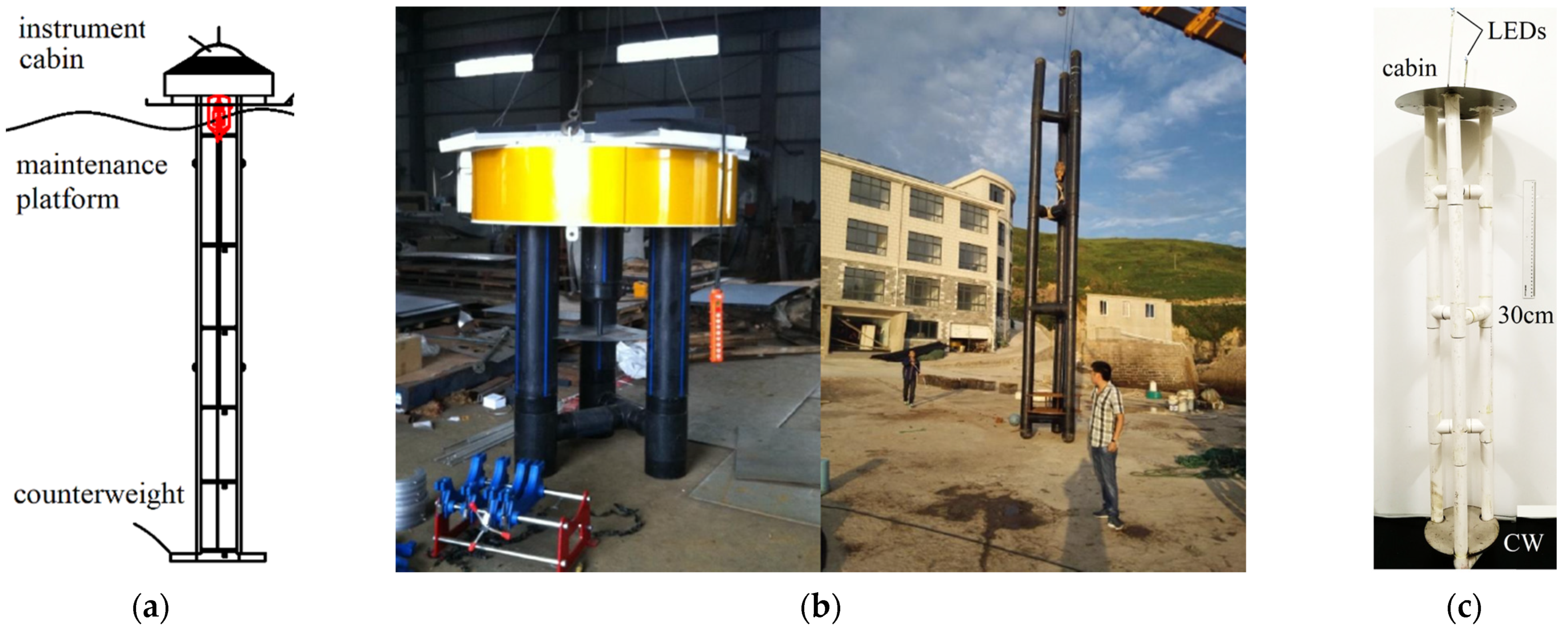
The experiment was carried out in the hydrodynamic laboratory of Zhejiang Ocean University. The scale of the experiment tank is 115 × 6.5 × 3.5 m. The maximum wave making is 30 cm, and the wave period is 0.5~2.0 s. The instruments used in the experiment include the wave-height gauge (type of BG-100, accuracy of 1 mm, made in Tianjin, China), the tension sensor (type of JLBS-P1, accuracy of 0.1% F·S, made in Bengpu, China), and the CCD image collection system (type of GL-JR-5, maximum shooting frequency of 1000 Hz, made in Qingdao, China). As shown in Figure 1, according to the principle of geometric similarity, the three-cylinder buoy is made of PVC pipe according to the scale of 1:7.8. Limited by the experiment conditions, the mass of the PVC floating three-cylinder frame is greater the prototype after gravity reduction. Therefore, taking the mass of the PVC floating frame as the reference standard, the quality of the cabin and the counterweight were designed according to the mass ratio of each part of the prototype [19].
The overall length of the prototype and model, the length of the three-way connection structure, and the relevant mass parameters are given in Table 1. The three-cylinder buoy included the floating frame, cabin, counterweight, and mooring cable. The most important feature of this buoy is that the pipelines for taking water in different water depths can be attached to the three-cylinder buoy to sample and monitor the water quality data at 25 m water depth.
2.2. Experiment Conditions
Using different wave conditions, the effects of wave heights and wave periods on the movement of the three-cylinder buoy and the tension of mooring cable were studied. Through field observation, Zhou et al. [20] obtained that the averagely significant wave height of the Donghai Sea offshore is 1.3 m (the physical model is 16.7 cm), the significant wave height of the 5% cumulative frequency is 3.0 m (the physical model is 38.5 cm), and the wave period is 1~5 s. Combined with the geometric scale of the buoy model and the wave making capacity of the tank, the experiment conditions were designed under the 2 groups of wave conditions. In the first group, the fixed wave period was 2.0 s, and the wave heights were divided into 5 values (10, 14, 18, 22, and 26 cm). For the other, the fixed wave height was 18 cm, and the wave periods were divided into 5 groups (1.6, 1.8, 2.0, 2.2, and 2.4 s). Waves with multiple heights and periods were selected to study the variation of hydrodynamic characteristics of the buoy model and the wave resistance of the buoy.
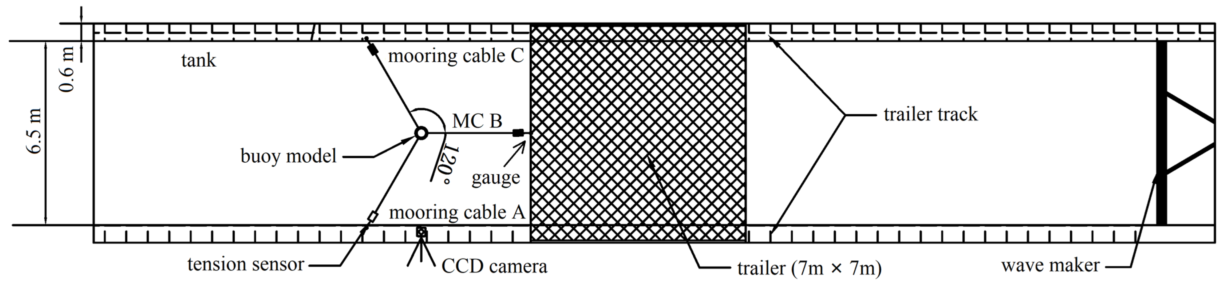
As shown in Figure 2, the buoy model with three mooring cables was tied at the angle of 120° and fixed in the center of the tank. The mooring cable of the wave front was mooring cable B. One side of the wave tank was mooring cable A, and the other was mooring cable C. The fixed ends of the three mooring cables were connected to each pulling force sensor. One wave height gauge was arranged at the tying point of mooring cable B and trailer. The wave height gauge was connected to the data collection system together with the pulling force sensor to realize the synchronous collection of wave height and tension. The CCD image collection system was arranged directly below the buoy, and the same computer was used for operation and collection. Therefore, a collection device integrating the movement of the buoy, the tension of the mooring cable, and the wave height was formed. After the commissioning of the experiment equipment and various parameters, the wave maker started to make waves according to the experiment conditions 1 and 2. In addition, the data of wave height and the tension of mooring cable were synchronously collected. Finally, by using the CCD camera, the trajectory of the two light-emitting diodes on the buoy model was collected (Figure 1b).
2.3. Data Collection and Processing
2.3.1. CCD Image Collection
Two light-emitting diodes were mounted on the upper end of the buoy model. Before the experiment started, the diodes were debugged to ensure normal work and provide a stable light source. After the stable wave formed in the tank (about three waves pass through the buoy; at this time, the wave is still not formed at the end of the tank, and the wave is not affected by the secondary reflection), the tension was collected and the CCD camera opened to continuously collect 180 pages of 8-bit gray images. The two luminous points on the gray image were the instantaneous positions of the diodes at the upper end of the buoy. The trajectories of the buoy model were obtained by tracking and analyzing the light points in the gray image through self-developed image software [21]. As shown in Figure 3a, the image processing software obtained the point position of the trajectory in each frame through continuous tracking of two luminescent points in 180 gray images. The trajectories on both sides of the coordinate axis corresponded to the trajectories of the left and right tracing points, respectively. In the physical experiment, the time of track collection was 10 s, including the tracks of 4~5 complete trajectories. By averaging the trajectories in several complete cycles in Figure 3a, a clearer and more accurate trajectory was obtained, thereby reducing the experiment error, as shown in Figure 3b.
2.3.2. The Tension Collection of the Mooring Cables
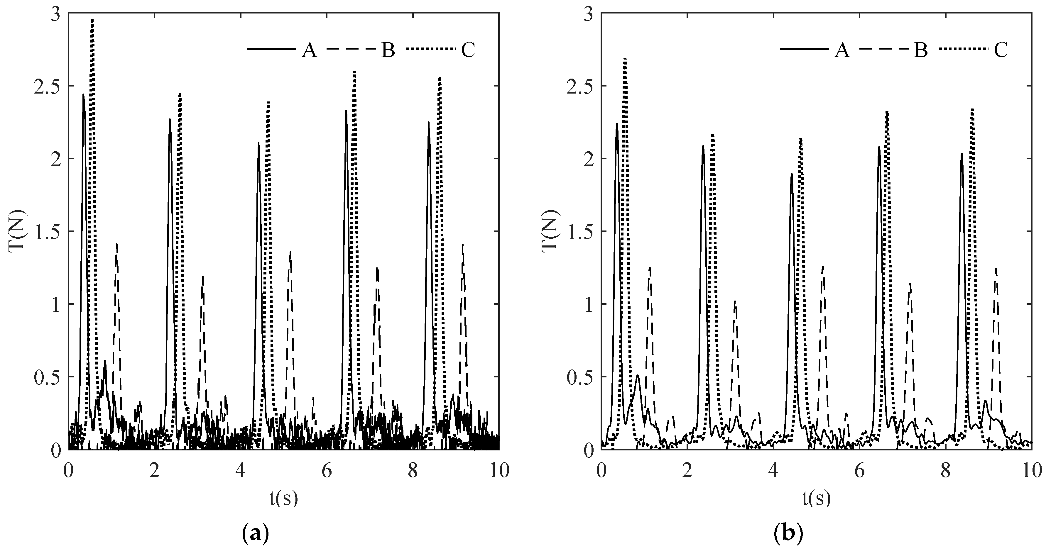
Firstly, when the wave maker started up and waited for 2~3, waves passed through the buoy model; then, we started to collect the forced data of the tension sensors on the three mooring cables and continuously collected the continuous data for 10 s each time. The wave height data collected by the wave height gauge were analyzed. If the accuracy of the preset wave height conditions was met, the data should be saved; otherwise, the physical experiment should be stared again. Ultimately, three repeated experiments satisfied the requirements of the experimental accuracy. Secondly, the average tension was regarded as the tension of mooring cable under the corresponding wave conditions. Figure 4a shows the source data of collected tension, and data burrs were handled by the fast Fourier transform algorithm. The fast Fourier transform is an efficient algorithm of discrete Fourier transform, which is widely used in image signal processing [22]. Finally, as shown in Figure 4b, the filtered data not only significantly reduced the burrs in the data but also ensured the objectivity of the data.
3. Experiment Results and Analysis
3.1. Analysis of Buoy Trajectory
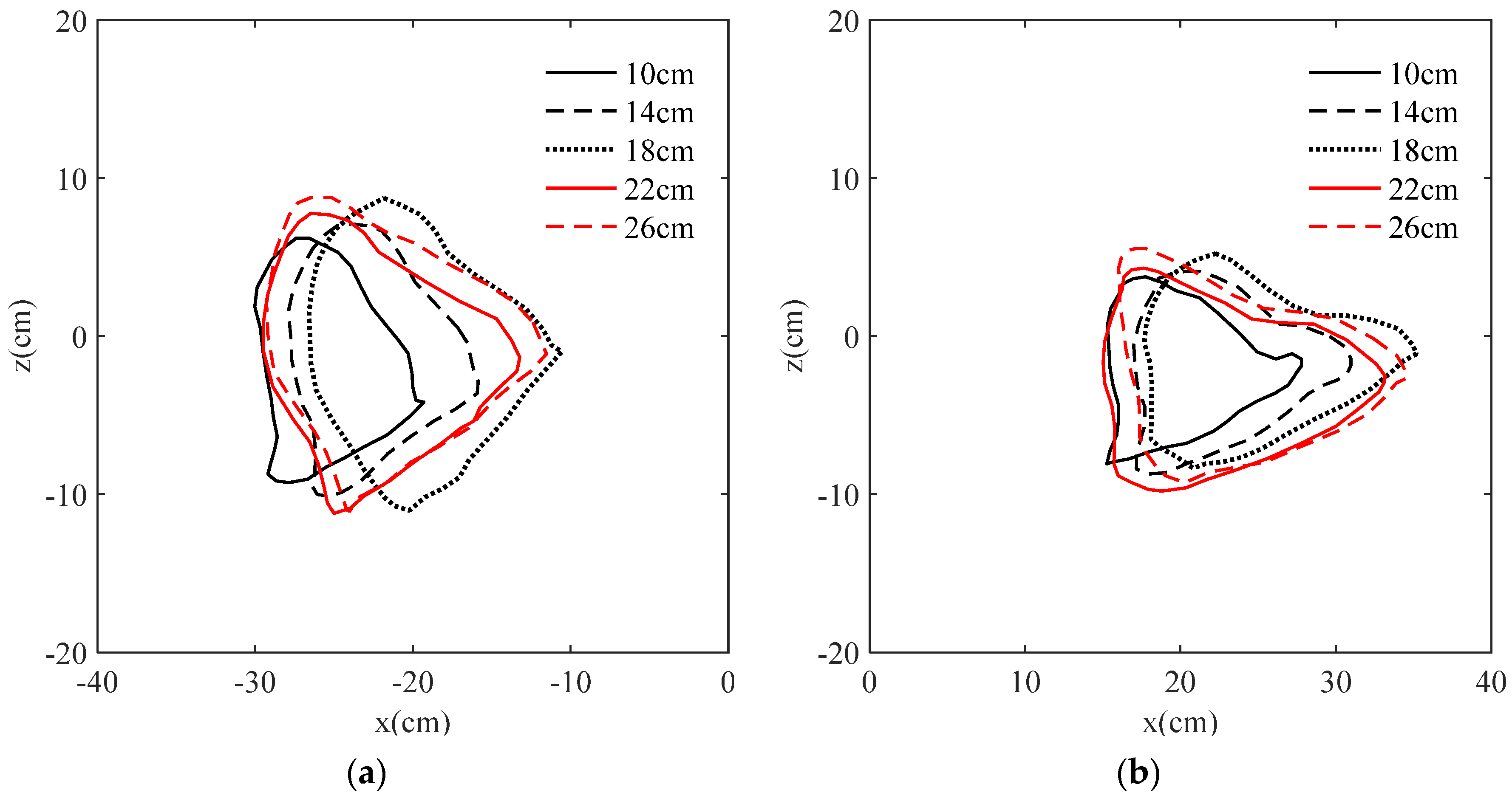
Figure 5a,b shows the trajectories of the left and the right tracer points under the conditions of the fixed period of 2.0 s and the wave heights of 10, 14, 18, 22, and 26 cm, respectively. The middle point of the two tracer points is the coordinate origin when the water surface was stationary. In general, the trajectory of the buoy was approximately elliptical. With the increased of the wave height, the right end of the trajectory of trace points on both sides increased to the positive direction of the x-axis, but the left end of the trajectory remained almost unchanged, and the positive and negative directions of the z-axis increased. Furthermore, the trajectory tended to move to the right under the influence of mooring cable B, and the trajectory became more and more “flat”.
Table 2 shows the characteristic values of the trajectory of the tracer points of the buoy model varying with the wave heights. In addition, Al and Ar represent the trajectory areas of the left and right tracer points, respectively; Lsl and Lsr indicate the left and right surging amplitudes, respectively; and Lhl and Lhr are the left and right heaving amplitudes, respectively. As shown in Table 2, firstly, with the increase of the wave height, the area of the trajectory increased, which reflected the strengthening of buoy movement. Meanwhile, the trajectory area corresponding to the left tracer point was larger than that of the right tracer point, which indicated that the change of the left tracer point was greater; however, when the wave height increased to 22 cm, the change of the trajectory area was smaller. Secondly, with the wave height increased, the surging amplitude of the buoy also increased. In addition, the motion law of the tracer points on both sides were essentially same. The surging amplitude increased significantly under the influence of wave heights from 10 to 18 cm. Moreover, it slowed down when the wave height reached 22 cm. Thirdly, from the minimum wave height to the maximum wave height, the surging amplitude of the left and right sides increased by 7 and 6 cm, respectively. Finally, with the increase of the wave height, the heaving amplitude of the buoy also increased. In particular, the left tracer point was more intense, and it increased by 4.4 cm, while the right tracer point was 3.0 cm. However, when the wave height was 22 cm, even the right tracer points decreased.
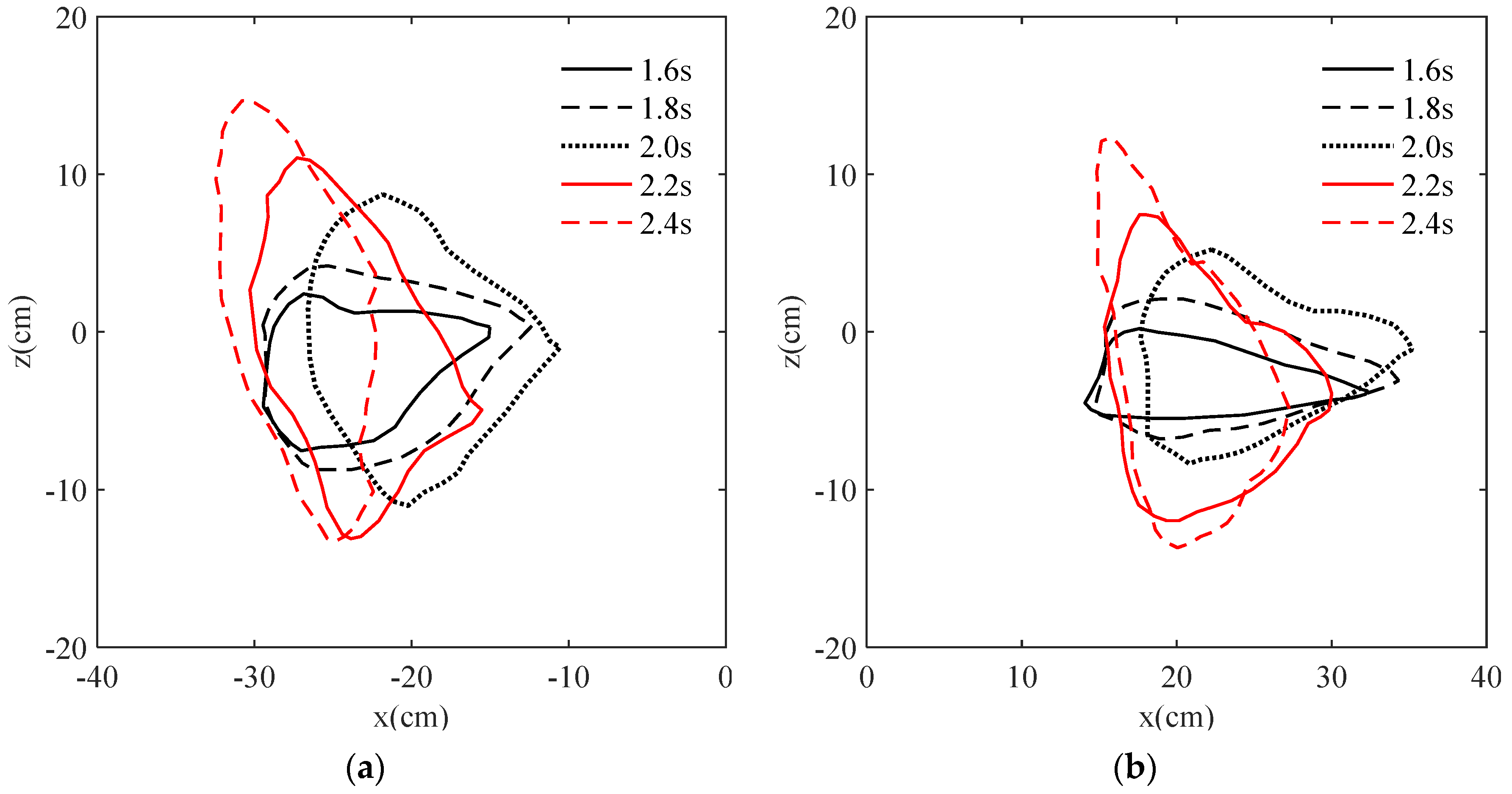
Figure 6 shows the trajectories of the left and right tracer points under the conditions of the fixed wave height of 18 cm and period of 1.6, 1.8, 2.0, 2.2, and 2.4 s. Firstly, we took the middle point of the two tracer points when the water surface was stationary as the coordinate origin. With the increase of the wave period, the right end of the trajectory of the tracer points on the left and the right sides firstly shifted to the positive direction of the x-axis. However, it shifted rapidly to the negative direction of the x-axis at the period of 2.2 s, the left end of the trajectory remained almost unchanged, and the trajectory clearly was offset in the positive and negative directions of the z-axis. Next, the trajectory of the buoy was approximately oval. Finally, with the increased of the wave period, the trajectory firstly shifted to the right and then to the left, and the trajectory also changed from “flat” to “narrow” under the influence of mooring cable B.
Table 3 showed that the characteristic values of the trajectory of the tracer points of the buoy model changed with the wave period. Firstly, with the increased of the wave period, the area included in the trajectory increased, which reflected the gradual strengthening of the buoy movement. Among them, the track area on the left tracer points did not continuously increase, but decreased when the period was 2.4 s. However, the right tracer points continuously increased, and the track area of the left tracer points were always greater than that of the right. Secondly, the variation law of surging amplitude at the tracer points on both sides was similar. The surging amplitude increased only when the period was 1.8 s, and then decreased. Thirdly, the surging amplitude on the right side was larger than the left side as a whole; meanwhile, the maximum difference of the surging amplitude on the right side was about 7.3 cm, and the left side was about 7.0 cm. Fourthly, the variation trend of heaving amplitude on the left and right tracer points was almost the same. With the increase of the wave period, the gradient increased. What is more, the heaving amplitude of the left tracer point was greater than the right tracer point. Finally, the heaving amplitude on left and right sides increased by about 20 cm.
3.2. Rolling Analysis of the Three-Cylinder Buoy
Figure 7a shows the statistics of the rolling angle of the buoy model under the 5 wave heights in experiment condition 1. The vertical direction was 0°. The left was positive, and the right was negative. The peak and trough values of the rolling angle corresponding to each wave height in Figure 7a were counted, and the average value was calculated as shown in Figure 7b. Under the fixed period of 2.0 s, the wave heights increased from 10 to 26 cm. The rolling angle was increased by about 2.6° in the positive direction, and about 2.2° in the negative. In addition, the peak values and trough values of the rolling angle were approximately on the same horizontal line. With the wave height increased, the rolling angle of the buoy did not change significantly, which indicated that the wave resistance was excellent.
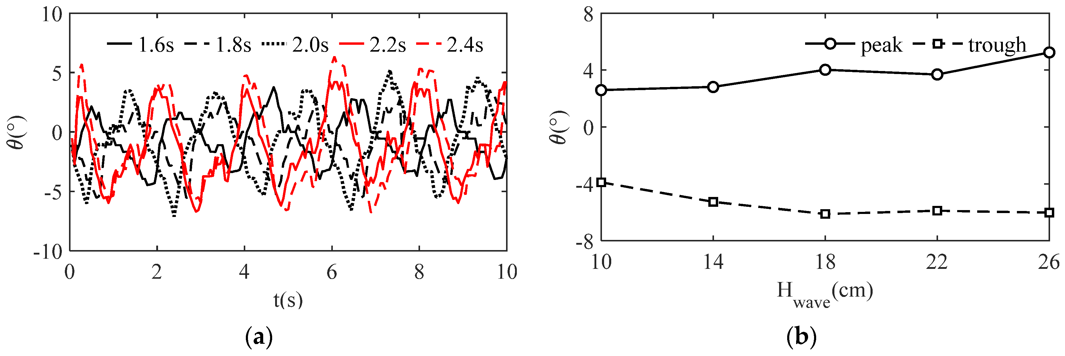
Figure 8a showed the statistics of the rolling angle of the buoy model under the wave periods in experiment condition 2. When the wave height was constant for 18 cm, the overall variation of the buoy rolling was not obvious with the increased of the period, and the difference between the peak value and trough value of the buoy rolling remained almost unchanged, up to about 10°. Consequently, it indicated that the rolling angle degree of the buoy in the horizontal direction was almost unchanged under the restraint of the mooring cable. In addition, the buoy would tilt slightly in the negative direction under the influence of the wave period.
3.3. Tension Analysis of the Mooring Cables
Figure 4b shows the average tension data of the mooring cables collected synchronously by three tension sensors at mooring cable terminals A, B, and C. Firstly, mooring cable A and mooring cable C were symmetrically distributed, so the tension was basically synchronous. However, due to the arrangement of the mooring cables and the measurement error of the tension sensor, there was less of a difference between the tension of mooring cable A and mooring cable C shown in Figure 4b, which had no impact on the analysis of the hydrodynamic characteristics of the buoy. Secondly, the tension of mooring cable B was significantly less than that of mooring cable A and mooring cable C, and the tension of mooring cable B had a second peak, which was related to the mooring pattern in Figure 2.
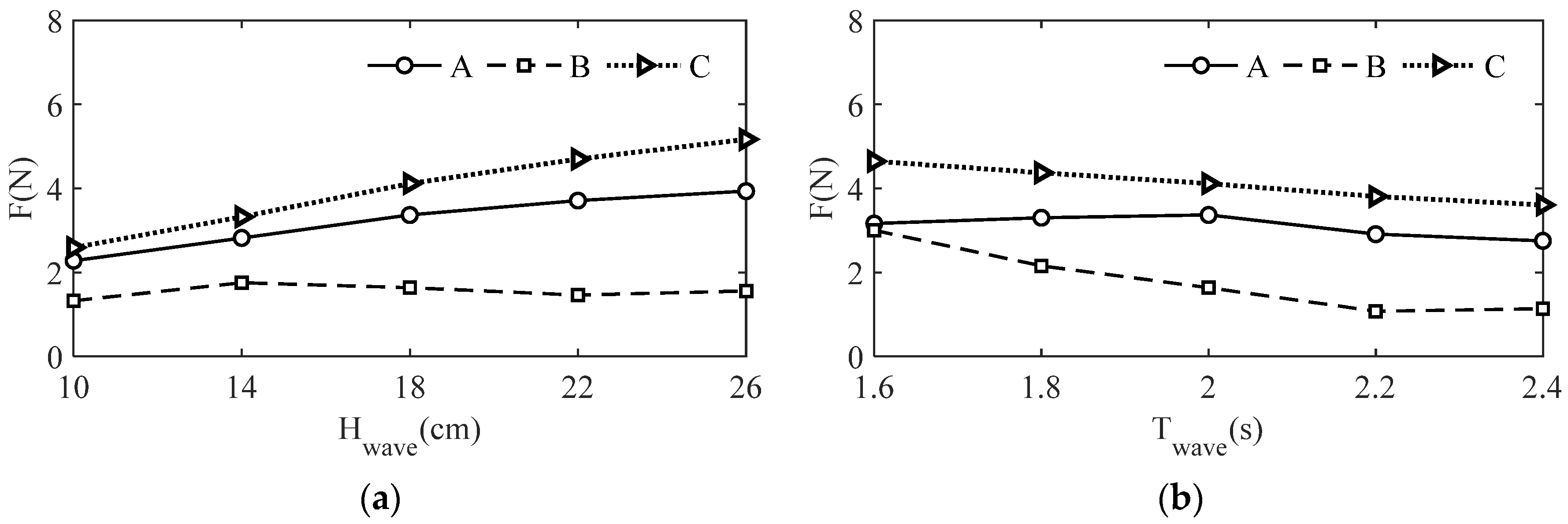
The tension of mooring cables was analyzed by the method of characteristic value. The average peak value of the tension of the mooring cables under each condition was selected as the characteristic value of the tension of the corresponding mooring cables. Table 4 shows the statistical results of characteristic value with wave height of 10 cm and period of 2.0 s. As shown in Figure 9, the influence of the wave height and the wave period on the maximum tension of the mooring cables was analyzed. Under different experiment conditions, the variation law of the maximum tension of mooring cable A and C were similar. With the wave heights increased from 10 cm to 26 cm, the tensions increased obviously, as shown in Figure 9a, but the gradients of tension increasing decreased. Furthermore, with the increased of the wave heights, the tension of mooring cable B remained almost unchanged and was not affected by the wave height. Moreover, from the analysis of the mooring cable tension, the resistance effect of the column buoy to wave height was obvious. Figure 9b shows that the tension of mooring cable A and mooring cable C decreased slowly as the period increased, and the maximum difference was only 0.8 N, while the tension of mooring cable B decreased gradually. Therefore, the mooring cable tension of the three-cylinder buoy was less affected by the wave period.
4. Numerical Model
The buoy system included the floating three-cylinder buoy, cabin, counterweight, and mooring cable, and it was necessary to calculate the wave force of each part of the system. Firstly, the fastened three-cylinder buoy mainly adopted the finite element method to calculate the force and moment around the center of mass of the three-cylinder buoy. Meanwhile, the translation and the rotation of the three-cylinder buoy were determined by discrete time. Secondly, the lumped mass point method was used to calculate the force on the flexible mooring cable and the tensile force after deformation. In the same way, discrete time was used to determine the movement speed and the spatial coordinates of the lumped mass point of the mooring cable.
4.1. Establishment Method
4.1.1. Simulation Method of the Three-Cylinder Buoy
- Wave force
The buoy structure mainly consists of a floating three-cylinder frame, a cabin, and a counterweight. Firstly, considering that the buoy was floating and the cabin was located above the water surface, the waves had no direct or less influence on the cabin. Therefore, it was considered possible to integrate the mass into the floating three-cylinder frame. Next, the counterweight was located at the bottom of the floating three-cylinder frame, which was of a smaller volume and had less wave influence on the entire buoy structure, and the mass was able to be integrated into the floating three-cylinder frame. Thus, to simplify the simulation, the whole buoy structure could be simplified into a floating three-cylinder frame.
The floating three-cylinder frame was a rigid structure. Under the action of waves, the floating three-cylinder frame was mainly affected by gravity, buoyancy, wave force, and the tension of the mooring cable. The movement of water mass points generated the wave force. Because of the velocity of water mass points gradually decreased from water surface to seabed, the wave force of the floating three-cylinder frame needed to be calculated using the finite unit method. The three-cylinder buoy of smaller diameter belonged to the small-scale category compared to the wave length, so the wave force could be calculated using the Morison equation. Thirdly, the hydrodynamic coefficient of the cylinder was directional and related to the relative movement velocity direction of the water particle [23]. When the floating three-cylinder frame rotates, the wave force of each unit should be calculated by considering the angle with the wave incident direction. Therefore, it was necessary to establish the local coordinate system. Above all, the detailed derivation and numerical simulations of the movement of the floating three-cylinder frame were studied [24].
- 2.
- Translation and rotation of the floating three-cylinder frame
Only considering translation, the forces of all units of the floating three-cylinder frame were accumulated in the global coordinate system. The acceleration of the floating three-cylinder frame was calculated by Newton’s second law, and the displacement per unit time step was analyzed by the fourth-order Runge–Kutta method [25]. Relative to the origin of the global coordinate system, the center of mass of the rigid structure in the global coordinate system was usually taken as the origin of the moving coordinate for rotation calculation. The movement of the floating three-cylinder frame not only included 3D translational movement, but also 3D rotational movement. A local coordinate system was established on the floating three-cylinder frame by referring to the principle of rigid structure dynamics, and then converting it to the global coordinate using the Blaine angle formula. The relevant formulas and theories could be found in the literature [24]. The center-of-mass coordinate and rotational inertia of the floating structure were deduced in this paper.
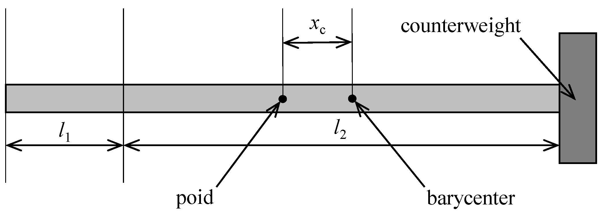
The floating three-cylinder frame is composed of three floating cylinders. The structure was relatively complex, and the calculation was difficult. In this simplified model, the floating three-cylinder frame was regarded as three independent floating cylinders, and the moment of inertia of each floating cylinder was considered separately. In order to ensure the water resistance of the floating three-cylinder frame, the cylinders were filled with the foam glue. Although the mass was very small, it was necessary to recalculate the density of the floating three-cylinder frame. As shown in Figure 10, l1 represents the length of the floating cylinder above the water surface, and l2 the depth of water inflow. rf indicates the radius of the floating cylinder, and rT the radius of the counterweight; lT is the thickness of the counterweight, and ρT is the density of the counterweight. ρf is the desired density of the floating cylinder. The formula is as follows:
As shown in Figure 10, the floating cylinder was regarded as a cylindrical structure with uniform medium, and its centroid was the geometric centroid. If a counterweight was added, the centroid will move down the length of xc. The size of xc can be calculated according to the following formulas, and the position of the centroid of the floating cylinder can be obtained.
According to the parallel axis theorem, the rotation inertia of the single floating cylinder in the three-axis was calculated as follows:
Figure 11 shows the density and centroid coordinates of the floating three-cylinder frame, which can be deduced by Formula (4), composed of three cylinders.
Figure 11 is the plan view of the floating three-cylinder frame. The centroid of the triangle was regarded as the origin from which to establish coordinate axis. The horizontal direction is the x-axis, and the vertical direction is the y-axis. According to the model parameters, the coordinates of points A, B, and C are (13.3/120.5, 13.3/2), (−13.3/120.5, 0), and (13.3/120.5, −13.3/2), respectively, Lr is the radius of the circumscribed circle of the plane triangle. According to the established coordinate system, the moment of inertia of the buoy in three axis was calculated by using the parallel axis theorem:
4.1.2. Simulation Method of the Mooring Cable
The mooring cable was a typical flexible structure that was simulated by the lumped mass method. Assuming that the mooring cable was composed of a finite massless spring connected by the lumped mass points, the shape of the mooring cable and the tension between each mass point were further obtained by calculating the offset of the lumped mass point under the influence on dynamic boundary conditions. The force of the lumped mass point of the mooring cable mainly included the gravity, the buoyancy, the tension of the mooring cable, the drag force, and the inertia force. The wave force received by the mooring cable could still be calculated using the Morrison formula. Firstly, the mooring cable mass point was regarded as a cylinder, and the calculation method of wave force was the same as the buoy; then, the particle movement equation was established by using Newton’s second law, as shown in Formula (6).
where l0 is the original length of the mooring cable, and l is the length after deformation. The unit was m. C1 and C2 represent the elastic coefficients of the mooring cables. d indicates the diameter of the mooring cable.
In the model experiment, it was difficult to tighten the three mooring cables and to ensure the preset water depth of the buoy. Therefore, the mooring cable had a certain degree of relaxation so that the water depth of the buoy could be ensured. This research proposed an efficient and accurate method to simulate the movement of the mooring cable in the non-tightened state. The initial position of the mass point of the mooring cable was designed by the position of tightened state. Then, when judging the tension of the mooring cable, the length l0 of ∆l in Formula (6) was increased. The mooring cable was freely able to move under no wave action, and the balanced state is the position of the mooring cable under the relaxed state. In particular, it was pointed out that the physical quantities in bold in Equation (6) were vectors in three directions of the global coordinate system (x, y, z), while the calculation of the tension T of the mooring cable was the physical quantity along the rope direction. It was necessary to calculate the projection under the overall coordinate system and convert it into T.
4.2. Establishment Method
Taking the working conditions of H = 22 cm, T = 2.0 s, d = 3.3 m (d is the water depth) as an example, the dynamic response of the three-cylinder buoy and the tension of mooring cables were obtained by the numerical simulation, and the result was compared with the physical experiment result.
4.2.1. Motion Status of the Three-Cylinder Buoy at Different Times
The numerical simulation should be able to describe the motion state of the buoy at different times. It was mainly verified by the initial state, the peak time, and the trough time of the buoy. Firstly, if three mooring cables were tightened at the same time in the physical experiment, the buoy would be lifted up, which did not meet the preset water entry depth of the buoy. Secondly, the initial position of the mooring cable was a straight line, and then the length ∆l of l0 was increased when judging the tension of the mooring cable. The free movement of the mooring cable under the condition of no wave was first conducted, and the equilibrium state of the mooring cable was the position under the relaxed state. As shown in Figure 12a, the three-cylinder buoy was in the tension state of the mooring cable, and Figure 12b was the equilibrium state of the buoy after natural movement under the relaxation state of the mooring cable. Figure 12c,d shows the movement state of the buoy and the tension distribution of mooring cable at the peak and trough time, respectively. It can be seen that the movement state of the buoy and mooring cable under wave action was well restored in the figure.
4.2.2. Comparison between the Trajectory of Tracing Points and the Tension of Mooring Cables
Figure 13a shows the trajectory of the floating three-cylinder frame under the designed condition. It can be seen from the figure that the trajectory of the three-cylinder buoy was approximately oval, and the shape was similar to the trajectory of the physical experiment under the same working condition. The surging and heaving amplitude were also similar. In the numerical simulation, the surging and heaving amplitude of the buoy were 17 and 21 cm respectively, which had a certain difference from the experiment results (about 3 cm). In general, the numerical simulation was in good agreement with the physical experiment. Therefore, the numerical simulation could reproduce the dynamic response of the three-cylinder buoy under wave action.
Due to the symmetrical arrangement of A and C mooring cables, there may be some asymmetric errors in physical experiments, but the tension values of the two mooring cables were completely equal in the numerical simulation, with the verification analysis thus only being for mooring cable A and B. Figure 13b,c shows the comparison results of the numerical simulation and the physical experiment of the mooring cable A and B, respectively. It can be seen from the figure that the simulation results of mooring cable A and B were well verified. The maximum tension was basically the same, and there was a slight difference in phase. However, only the second peak of the mooring cable B appeared, and the two peaks were almost equal in the model experiment., which requires further analysis and discussion.
The reason why the trajectory of the tracer point was slightly different may have have been due to an error in model making. Firstly, to ensure that the buoy model did not enter the water for a long period of time, the foam glue was filled in the cylinder, and it was not a homogeneous medium. Secondly, it was difficult to maintain the tension state of three mooring cables and the angle of 120° among them in the physical test. Last but not least, the three-way connection structure of the floating frame was not considered in the numerical simulation. Next, the numerical model will focus on solving the problem of the buoy structure of the three-way connection. The tension verification of the mooring cable of A shown in Figure 13b was good. The second peak value of tension shown in Figure 13c may have been caused by instrument failure, but the peak value of tension was in accordance with the value of numerical simulation.
5. Discussion
5.1. Physical Experiment
Through changing the wave elements, the hydrodynamic characteristics of the three-cylinder buoy fastened by three mooring cables were studied. The trajectory of the three-cylinder buoy was directly relevant to the wave factors. However, the trajectory on the right tracer point was always smaller than the left in terms of the area and heaving, and only the surging was larger than that of the left, which was related to the tying method of the three mooring cables used in the physical experiment (Figure 2). The mooring cable B was parallel to the wave propagation direction, which led to a larger vertical constraint. Therefore, the trajectory on the right tracer point showed a horizontal movement. With the increased of the wave height, the maximum variation of the rolling angle was no more than 3° through analyzing the rolling of the three-cylinder buoy, and the surging amplitude on the left and right sides increased by about 7 and 6 cm, respectively. In addition, the heaving amplitude increased by about 4.4 and 3.0 cm. Moreover, the influence of wave heights on the surging amplitude of the three-cylinder buoy was greater than the heaving amplitude. It was further confirmed that the wave resistance of the three-cylinder buoy was very superior. Additionally, with the wave period increased, the difference of the rolling angle in the positive and negative directions was almost unchanged; in other words, the rolling of the buoy in the horizontal direction was almost unchanged, yet there was a slight shifting to one side. When the wave height was 18 cm, the maximum difference between left and right surging was 7.0 and 7.3 cm, respectively, and the left and right heaving increased by about 20 cm. Obviously, the influence of period on the heaving of the three-cylinder buoy far outweighed the surging. To sum up, the three-cylinder buoy had strong wave resistance and certain stability, and what is more, the accurate acquisition of water samples at the target water depth could also be ensured. The stability of the three-cylinder buoy was sensitive to the wave period, and the large wave period could cause the buoy to fluctuate with large amplitude in the vertical direction.
In the fixed wave period (2.0 s), the movement of the three-cylinder buoy model strengthened, and the tension of mooring cable increased with the increased of the wave height, but the tension growth rate of the mooring cable was slow. The tension of mooring cable A and mooring cable C changed synchronously, and the values were slightly different. The maximum difference was 1.1 N. The tension of mooring cable B was much less than that of mooring cable A and mooring cable C, and the tension was less affected by wave height (<0.5 N). Since the tension of mooring cable A and mooring cable C were greater than the mooring cable B, the left half of the trajectory shown in Figure 5a,b was significantly stronger than the right half. The conception of the momentum is that the change of momentum was equal to the product of the wave force F and the action time t. In Table 5, it is assumed that the buoy mass remained unchanged, the average velocity v of the buoy within the sampling time interval was calculated according to the trajectory data, and the maximum wave force was obtained. The maximum wave force was indirectly calculated from the trajectory data. Compared with the measured wave force of the tension sensor, the rule that the maximum wave force was less affected by the wave height was also obtained, and then the tension of the mooring cable B on the wave front was related to the variation of buoy momentum, which was unable to be explained only by the wave height. In the physical experiment, the wave propagation direction was parallel to the mooring cable B. Due to the experiment conditions, the influence of the wave propagation direction on the tension of mooring cables was not further studied. According to the existing experiment results and conclusions, the three-cylinder buoy and mooring cables could be adjusted by the motion law under current and wave action in the actual sea area.
In the fixed wave height (18 cm), the movement of the buoy model weakened with the increased of the wave period. The tension of mooring cable A and mooring cable C decreased slowly in a stepwise manner, and the maximum difference was about 0.5 N. However, the tension of mooring cable B decreased significantly, and the maximum difference was about 2 N. Afterwards, the tension variation law of mooring cable A and mooring cable C was similar, but the values were slightly different. The maximum difference was 1.3 N. The tension of the mooring cable B was almost unchanged in experiment condition 1, but it showed a completely opposite law in experiment condition 2. As shown in Table 6, the maximum wave force acting on the buoy decreased continuously, which was calculated by the formula of the momentum, and the mooring cable tension measured by the corresponding tension sensor also decreased significantly. Comprehensively analyzing the tension variation of mooring cable B in the two experiment conditions, the wave period in experiment condition 1 remained unchanged, and the tension variation of the mooring cable was not obvious. In addition, the wave period in experiment condition 2 became larger, and the tension of mooring cable decreased significantly. It was found that the wave period played a major role in the tension of mooring cable B, rather than the wave height.
5.2. Numerical Simulation
The initial state of the mooring cable was an ideal state (Figure 12a), and the mooring cable was tensioned (in a straight line). There was no tension between the mooring cable and the three-cylinder buoy, which was difficult to achieve in the physical experiment. Therefore, in the model experiment, the buoy would rise and deviate from the preset water entry depth when the mooring cable was tensioned, and the tightness of the mooring cable would greatly affect the result of the tension. To solve this problem, Zhu et al. [26,27,28] simulated the initial state of the mooring cable by fitting the trajectory line of the mooring cable, and then the mass points were added on the trajectory. However, this method is time-consuming and inaccurate. As shown in Figure 12b, it was proposed that a small reserved length to the mooring cable in the critical state was added to make its natural movement reach the equilibrium state without applying external force. As shown in Figure 12c,d, the simulation results of the tension of the mooring cable A and B were basically consistent with the results of the model experiment.
Under the wave condition of wave height of 22 cm and period of 2.0 s, the numerical simulation of the movement of the three-cylinder buoy and the tension of the mooring cable were in good agreement with the model experiment results. Nevertheless, the results were still slightly different, and the main reasons for the difference were as follows:
- In the model experiment, it was difficult to unify the relaxation degree of the three mooring cables, which was avoided by setting parameters in the numerical simulation.
- In the numerical simulation, the static state of the three-cylinder buoy (water entry depth) was taken as the premise. The three-cylinder buoy was regarded as a homogeneous medium to calculate the theoretical density. However, to ensure the water resistance of the buoy, the foam glue, which is not a homogeneous medium, was filled in the cylinder in the physical experiment.
- Due to the complexity of the structure, the three-way connection structure of the floating three-cylinder frame was not considered in the numerical simulation, which resulted in some differences in the movement of the system. On the basis of the analysis of the above reasons and the verification of the results, it could be concluded that the simulation method proposed in this paper was feasible.
6. Conclusions
This paper studied the influence of wave on the movement of the three-cylinder buoy and the tension of mooring cables at different wave heights and periods through the model experiment. The following conclusions were obtained: (1) With the increase in the wave height, the surging amplitude, the heaving amplitude, and the rolling angle of the three-cylinder buoy, there was an increase of a small gradient, and the three-cylinder buoy showed strong adaptability to different wave heights, which can ensure certain stability and the accurate acquisition of the water sample in the target water depth. The stability of the three-cylinder buoy is more sensitive to the wave period, and the large wave period can lead to a large rise and fall of the three-cylinder buoy in the vertical direction. (2) With the increase of the wave height, the tension of the mooring cables increased. However, the growth rate of the tension of mooring cables was slower. As the period increased, the tension of mooring cables decreased to different degrees. (3) The change rate of the buoy momentum can reasonably explain the variation law of the mooring cables on the wave front, and the wave period had a great influence in the tension of mooring cables, rather than the wave height. (4) The numerical model of the floating three-cylinder frame and the mooring cables was established by using the finite element method and lumped mass point method. The trajectory of tracer point and the tension of the mooring cables were verified under experiment condition 1. Firstly, the numerical method of the three-cylinder buoy and the method of the initial state of the mooring cable by increasing the reserved length were proposed. Secondly, the force formulas of the floating three-cylinder frame and the mooring cable were given, and the accuracy of the numerical simulation method was verified with the conclusions of the physical experiment. Finally, a numerical simulation method of the fastened three-cylinder buoy was provided.
Author Contributions
Conceptualization, methodology, and writing—original draft preparation, Y.P. and D.X.; writing—review and checking, F.Y. and H.T.; project administration and funding acquisition, C.L. and X.Z.; visualization, D.X. and L.S. All authors have read and agreed to the published version of the manuscript.
Funding
This research was funded by the provincial scientific research fund for basic research of China (2021JZ008) and the National Natural Science Foundation of China (no. 52101330).
Institutional Review Board Statement
Not applicable.
Informed Consent Statement
Not applicable.
Data Availability Statement
Not applicable.
Acknowledgments
We would like to thank the financial support of the provincial scientific research fund for basic research of China (2021JZ008) and the National Natural Science Foundation of China (no. 52101330). The authors would like to express profound thanks to them.
Conflicts of Interest
The authors declare no conflict of interest.
References
- Wang, J.; Wang, Z.; Wang, Y.; Liu, S.; Li, Y. Current situation and trend of marine data buoy and monitoring network technology of China. Acta Oceanol. Sin. 2016, 35, 1–10. [Google Scholar] [CrossRef]
- Qian, C.; Huang, B.; Yang, X.; Chen, G. Data science for oceanography: From small data to big data. Big Earth Data 2021, 1–15. [Google Scholar] [CrossRef]
- Schmidt, W.; Raymond, D.; Parish, D.; Ashton, I.G.; Miller, P.I.; Campos, C.J.; Shutler, J.D. Design and operation of a low-cost and compact autonomous buoy system for use in coastal aquaculture and water quality monitoring. Aquac. Eng. 2018, 80, 28–36. [Google Scholar] [CrossRef]
- Loverich, G.; Forster, J. Advances in offshore cage design using spar buoys. Mar. Technol. Soc. J. 2000, 34, 18–28. [Google Scholar] [CrossRef]
- Gui, F.; Wang, P.; Pan, Y.; Feng, D.; Zuo, X. Cylindrical Anti Wind and Wave Marine Stratified Sampling Water Quality Monitoring Buoy. Chinese Patent CN108168957B, 16 June 2020. [Google Scholar]
- Shi, Q.; Wang, H.; Wu, H.; Lee, C. Self-powered triboelectric nanogenerator buoy ball for applications ranging from environment monitoring to water wave energy farm. Nano Energy 2017, 40, 203–213. [Google Scholar] [CrossRef]
- Amaechi, C.V.; Wang, F.; Ye, J. Numerical studies on CALM buoy motion responses and the effect of buoy geometry cum skirt dimensions with its hydrodynamic waves-current interactions. Ocean Eng. 2022, 244, 110378. [Google Scholar] [CrossRef]
- Ryu, S.; Duggal, A.S.; Heyl, C.N.; Liu, Y. Coupled analysis of deepwater oil offloading buoy and experimental verification. In Proceedings of the Fifteenth International Offshore and Polar Engineering Conference, Seoul, Korea, 19–24 June 2005. [Google Scholar]
- Ryu, S.; Duggak, A.S.; Heyl, C.N. Prediction of deep water oil offloading buoy response and experimental validation. Int. J. Offshore Polar Eng. 2006, 16, 290–296. [Google Scholar]
- Touzon, I.; Nava, V.; Gao, Z.; Petuya, V. Frequency domain modelling of a coupled system of floating structure and mooring Lines: An application to a wave energy converter. Ocean Eng. 2021, 220, 108498. [Google Scholar] [CrossRef]
- Jin, C.; Kang, H.; Kim, M.; Cho, I. Performance estimation of resonance-enhanced dual-buoy wave energy converter using coupled time-domain simulation. Renew. Energy 2020, 160, 1445–1457. [Google Scholar] [CrossRef]
- Salem, A.G.; Ryu, S.; Duggal, A.S.; Datla, R.V. Linearization of quadratic drag to estimate calm buoy pitch motion in frequency-domain and experimental validation. J. Offshore Mech. Arct. Eng. 2012, 134, 011305. [Google Scholar] [CrossRef]
- Amaechi, C.V.; Wang, F.; Ye, J. Investigation on Hydrodynamic Characteristics, Wave–Current Interaction and Sensitivity Analysis of Submarine Hoses Attached to a CALM Buoy. J. Mar. Sci. Eng. 2022, 10, 120. [Google Scholar] [CrossRef]
- Yang, K.; Abdelkefi, A.; Li, X.; Mao, Y.; Dai, L.; Wang, J. Stochastic analysis of a galloping-random wind energy harvesting performance on a buoy platform. Energy Convers. Manag. 2021, 238, 114174. [Google Scholar] [CrossRef]
- Le Cunff, C.; Ryu, S.; Duggal, A.; Ricbourg, C.; Heurtier, J.M.; Heyl, C.; Beauclair, O. Derivation of calm buoy coupled motion raos in frequency domain and experimental Validation. In Proceedings of the Seventeenth International Offshore and Polar Engineering Conference, Lisbon, Portugal, 1–6 July 2007. [Google Scholar]
- Zhu, X.; Yoo, W.S. Dynamic analysis of a floating spherical buoy fastened by mooring cables. Ocean Eng. 2016, 121, 462–471. [Google Scholar] [CrossRef]
- Chen, F.; Duan, D.; Han, Q.; Yang, X.; Zhao, F. Study on force and wave energy conversion efficiency of buoys in low wave energy density seas. Energy Convers. Manag. 2019, 182, 191–200. [Google Scholar] [CrossRef]
- Amaechi, C.V.; Wang, F.; Hou, X.; Ye, J. Strength of submarine hoses in Chinese-lantern configuration from hydrodynamic loads on CALM buoy. Ocean Eng. 2019, 171, 429–442. [Google Scholar] [CrossRef] [Green Version]
- Wu, C.W.; Gui, F.K.; Li, Y.C.; Fang, W.H. Hydrodynamic coefficients of a simplified floating system of gravity cage in waves. J. Zhejiang Univ.-Sci. A 2008, 9, 654–663. [Google Scholar] [CrossRef]
- Zhou, Y.; Li, Z.; Pan, Y.; Bai, X.; Wei, D. Distribution characteristics of waves in Sanmen Bay based on field observation. Ocean Eng. 2021, 229, 108999. [Google Scholar] [CrossRef]
- Feng, D.; Meng, A.; Wang, P.; Yao, Y.; Gui, F. Effect of design configuration on structural response of longline aquaculture in waves. Appl. Ocean Res. 2021, 107, 102489. [Google Scholar] [CrossRef]
- Greengard, L.; Lee, J.Y. Accelerating the nonuniform fast Fourier transform. SIAM Rev. 2004, 46, 443–454. [Google Scholar] [CrossRef] [Green Version]
- Geng, B.L.; Teng, B.; Ning, D.Z. A time-domain analysis of wave force on small-scale cylinders of offshore structures. J. Mar. Sci. Technol. 2010, 18, 12. [Google Scholar] [CrossRef]
- Pan, Y.; Tong, H.; Zhou, Y.; Liu, C.; Xue, D. Numerical Simulation Study on Environment-Friendly Floating Reef in Offshore Ecological Belt under Wave Action. Water 2021, 13, 2257. [Google Scholar] [CrossRef]
- Liu, Y.; Dou, C.; Sun, Q.; Xu, Q. Optimal control of path tracking for vehicle-handling dynamics. SAE Int. J. Passeng. Cars-Mech. Syst. 2020, 13, 225–243. [Google Scholar] [CrossRef]
- Zhu, X.; Yoo, W.S. Flexible dynamic analysis of an offshore wind turbine installed on a floating spar platform. Adv. Mech. Eng. 2016, 8. [Google Scholar] [CrossRef] [Green Version]
- Zhu, X.; Wang, Y.; Yu, K.; Pei, Y.; Wei, Z.; Zong, L. Dynamic analysis of deep-towed seismic array based on relative-velocity-element-frame. Ocean Eng. 2020, 218, 108243. [Google Scholar] [CrossRef]
- Zhu, X.; Yoo, W.S. Numerical modeling of a spherical buoy moored by a cable in three dimensions. Chin. J. Mech. Eng. 2016, 29, 588–597. [Google Scholar] [CrossRef]
Figure 1.
The structure diagram of the three-cylinder buoy. (a) The design of the model. (b) A diagram of the buoy prototype. (c) A diagram of a buoy model.
Figure 1.
The structure diagram of the three-cylinder buoy. (a) The design of the model. (b) A diagram of the buoy prototype. (c) A diagram of a buoy model.

Figure 2.
The schematic of the physical experiment.

Figure 3.
Average processing on the trajectory of tracing point. (a) The trajectory of tracer point. (b) The trajectory after averaging.
Figure 3.
Average processing on the trajectory of tracing point. (a) The trajectory of tracer point. (b) The trajectory after averaging.

Figure 4.
Data filtering schematic of tension. (a) Data before filtering. (b) Filtered data.

Figure 5.
The trajectory of the tracer points (experiment condition 1). (a) On the left. (b) On the right.
Figure 5.
The trajectory of the tracer points (experiment condition 1). (a) On the left. (b) On the right.

Figure 6.
The trajectory of the tracer points (experiment condition 2). (a) On the left. (b) On the right.
Figure 6.
The trajectory of the tracer points (experiment condition 2). (a) On the left. (b) On the right.

Figure 7.
Variation of the rolling angle (experiment condition 1). (a) With time. (b) With wave heights.
Figure 7.
Variation of the rolling angle (experiment condition 1). (a) With time. (b) With wave heights.

Figure 8.
Variation of the rolling angle (experiment condition 2). (a) With time. (b) With wave heights.
Figure 8.
Variation of the rolling angle (experiment condition 2). (a) With time. (b) With wave heights.

Figure 9.
Variation of mooring cable tensions in experiment conditions 1 and 2. (a) With the wave height. (b) With the wave period.
Figure 9.
Variation of mooring cable tensions in experiment conditions 1 and 2. (a) With the wave height. (b) With the wave period.

Figure 10.
Schematic of the centroid of floating cylinder.

Figure 11.
The structure diagram of floating three-cylinder frame. (a) Plane graph and aspect ratio. (b) Model diagram.
Figure 11.
The structure diagram of floating three-cylinder frame. (a) Plane graph and aspect ratio. (b) Model diagram.

Figure 12.
Digital simulation results of the buoy fastened by 3 mooring cables. (a) Mooring cable in tightened state. (b) Mooring cable in initial state. (c) The motion state of the buoy under wave peak. (d) The motion state under wave trough.
Figure 12.
Digital simulation results of the buoy fastened by 3 mooring cables. (a) Mooring cable in tightened state. (b) Mooring cable in initial state. (c) The motion state of the buoy under wave peak. (d) The motion state under wave trough.

Figure 13.
The result comparison between the numerical simulation and physical experiment. (a) The trajectory. (b) The tension of mooring cable A. (c) The tension of mooring cable B.
Figure 13.
The result comparison between the numerical simulation and physical experiment. (a) The trajectory. (b) The tension of mooring cable A. (c) The tension of mooring cable B.


Table 1.
Main parameters of the prototype buoy and model buoy.
| Parameters | Prototype | Model |
|---|---|---|
| Length of the buoy/m | 8.47 | 1.08 |
| Length of the three-way connection structure/m | 1.25 | 0.166 |
| Mass of the three-cylinder frame/kg | 363.5 | 1.215 |
| Buoyancy of the three-cylinder frame/kg | 1297.4 | 2.749 |
| Mass of the cabin/kg | 260 | 0.374 |
| Mass of the counterweight/kg | 914.8 | 1.315 |
Table 2.
The characteristic value of the trajectory the tracer points (experiment condition 1).
| Wave Height/cm | Area Lp/cm2 | Area Rp/cm2 | Surging Lp/cm * | Heaving Lp/cm | Surging Rp/cm * | Heaving Rp/cm |
|---|---|---|---|---|---|---|
| 10 | 105.986 | 86.712 | 10.723 | 15.474 | 12.515 | 11.834 |
| 14 | 131.083 | 111.778 | 12.045 | 17.229 | 13.965 | 12.816 |
| 18 | 191.362 | 141.817 | 16.029 | 19.754 | 17.511 | 13.582 |
| 22 | 181.677 | 163.482 | 16.265 | 18.974 | 18.165 | 14.113 |
| 26 | 204.631 | 165.236 | 17.755 | 19.879 | 18.559 | 14.804 |
* Lp represents the left tracer points, and Rp represents the right.
Table 3.
The characteristic values of the trajectory of tracer points (experiment condition 2).
| Period/s | Area Lp/cm2 | Area Rp/cm2 | Surging Lp/cm | Heaving Lp/cm * | Surging Rp/cm * | Heaving Rp/cm |
|---|---|---|---|---|---|---|
| 1.6 | 90.9113 | 65.0382 | 14.428 | 9.961 | 18.217 | 5.691 |
| 1.8 | 152.8007 | 110.1839 | 17.157 | 12.925 | 19.635 | 8.871 |
| 2.0 | 191.3615 | 141.817 | 16.029 | 19.754 | 17.511 | 13.582 |
| 2.2 | 192.5868 | 171.9369 | 14.753 | 24.168 | 14.667 | 19.415 |
| 2.4 | 182.4064 | 174.2035 | 10.186 | 27.949 | 12.396 | 25.942 |
* Lp represents the left tracer points, and Rp represents the right.
Table 4.
Peak value of the tension of the mooring cables.
| Mooring Cables | n1/N | n2/N | n3/N | n4/N | n5/N | Average/N |
|---|---|---|---|---|---|---|
| Mooring cable A | 2.44 | 2.27 | 2.11 | 2.23 | 2.35 | 2.28 |
| Mooring cable B | 1.41 | 1.19 | 1.36 | 1.27 | 1.41 | 1.328 |
| Mooring cable C | 2.96 | 2.45 | 2.39 | 2.6 | 2.56 | 2.592 |
Table 5.
Variation of maximum wave force (experiment condition 1).
| Wave Height/cm | 10 | 14 | 18 | 22 | 26 |
| Wave force/N | 2.915 | 2.999 | 2.925 | 2.999 | 2.929 |
Table 6.
Variation of maximum wave force (experiment condition 2).
| Period/s | 1.6 | 1.8 | 2.0 | 2.2 | 2.4 |
| Wave force/N | 4.536 | 4.088 | 3.516 | 3.005 | 2.959 |
Publisher’s Note: MDPI stays neutral with regard to jurisdictional claims in published maps and institutional affiliations. |
© 2022 by the authors. Licensee MDPI, Basel, Switzerland. This article is an open access article distributed under the terms and conditions of the Creative Commons Attribution (CC BY) license (https://creativecommons.org/licenses/by/4.0/).
Share and Cite
MDPI and ACS Style
Pan, Y.; Yang, F.; Tong, H.; Zuo, X.; Shen, L.; Xue, D.; Liu, C. Experimental and Numerical Simulation of a Symmetrical Three-Cylinder Buoy. Symmetry 2022, 14, 1057. https://0-doi-org.brum.beds.ac.uk/10.3390/sym14051057
AMA Style
Pan Y, Yang F, Tong H, Zuo X, Shen L, Xue D, Liu C. Experimental and Numerical Simulation of a Symmetrical Three-Cylinder Buoy. Symmetry. 2022; 14(5):1057. https://0-doi-org.brum.beds.ac.uk/10.3390/sym14051057
Chicago/Turabian StylePan, Yun, Fengting Yang, Huanhuan Tong, Xiao Zuo, Liangduo Shen, Dawen Xue, and Can Liu. 2022. "Experimental and Numerical Simulation of a Symmetrical Three-Cylinder Buoy" Symmetry 14, no. 5: 1057. https://0-doi-org.brum.beds.ac.uk/10.3390/sym14051057
Note that from the first issue of 2016, this journal uses article numbers instead of page numbers. See further details here.