
Image Segmentation via Multiscale Perceptual Grouping

College of Computer Science, Sichuan University, Chengdu 610065, China
*
Author to whom correspondence should be addressed.
Symmetry 2022, 14(6), 1076; https://0-doi-org.brum.beds.ac.uk/10.3390/sym14061076
Submission received: 12 April 2022
/
Revised: 17 May 2022
/
Accepted: 19 May 2022
/
Published: 24 May 2022
(This article belongs to the Special Issue Symmetry in Image Processing and Visualization)
Abstract
:The human eyes observe an image through perceptual units surrounded by symmetrical or asymmetrical object contours at a proper scale, which enables them to quickly extract the foreground of the image. Inspired by this characteristic, a model combined with multiscale perceptual grouping and unit-based segmentation is proposed in this paper. In the multiscale perceptual grouping part, a novel total variation regularization is proposed to smooth the image into different scales, which removes the inhomogeneity and preserves the edges. To simulate perceptual units surrounded by contours, the watershed method is utilized to cluster pixels into groups. The scale of smoothness is determined by the number of perceptual units. In the segmentation part, perceptual units are regarded as the basic element instead of discrete pixels in the graph cut. The appearance models of the foreground and background are constructed by combining the perceptual units. According to the relationship between perceptual units and the appearance model, the foreground can be segmented through a minimum-cut/maximum-flow algorithm. The experiment conducted on the CMU-Cornell iCoseg database shows that the proposed model has a promising performance.
1. Introduction
Image segmentation is used to split pixels of an image into different symmetrical or asymmetrical regions—especially semantic objects. In the past few decades, researchers have proposed a large number of segmentation algorithms based on the image features, such as the edges [1], intensity/color distributions [2], and texture [3]. However, these features are sensitive to inhomogeneity, illumination, and other negative factors; therefore, image segmentation is still a challenging task.
The foreground and background segmentation are carried out to divide an image into two semantic parts based on its features. The features applied in the existing image segmentation can be divided into two categories: learned features and low-level features. The learned features are obtained from training data via machine learning methods [4,5]. The feature-extraction ability is sensitive to the training data and their capacity, leading to poor segmentation performance for new categories that do not appear in the training data. In practice, the capacity of the training data is limited [6]. Low-level features are mathematical representations of intensity/color similarity, local variation in intensity/color, statistical characteristics, and distribution models of region intensity/color. The acquisition of these features only requires analysis of several images without training. However, the low-level features are sensitive to intensity/color inhomogeneity, which leads to poor segmentation results for images of nature by such methods [7]. For example, the slow intensity/color changes at the boundary of two adjacent objects will result in poor segmentation accuracy [7]. The parameter estimation of the region’s intensity/color distribution will become inaccurate for the inhomogeneous regions [8].
The human eyes can quickly extract the foreground of an image. The reason for this is that the eyes observe an image as perceptual groups instead of discrete pixels, and extract features from proper scales. Inspired by this characteristic, we propose a multiscale perceptual grouping segmentation model. The model consists of multiscale perceptual grouping and perceptual-unit-based segmentation. In the multiscale perceptual grouping part, a novel method is designed to smooth inhomogeneity and preserve the edges of the image. In each smoothed image, the pixels are grouped into perceptual units for the selection of proper scale and segmentation. In the perceptual-unit-based segmentation part, a unit-based graph-cut method is designed. This method utilizes KL divergence to measure the relationships between perceptual units. The experimental results show that the model proposed in this paper has a competitive performance.
2. Related Works
The performance of the segmentation algorithms not only depends on the algorithm itself, but also varies with the features. Much effort in the image segmentation research is devoted to feature extraction and representation, such as regional coherence [9], edge smoothness [7], and visual homogeneity [10]. Segmentation results of representative methods are shown in Figure 1.
The deep learning methods extract features and build pixel-wise classifiers by training the parameters of neural networks, such as fully convolution networks (FCNs) [4,15,16,17], DeepLab [5,18], etc. These methods achieve competitive performance for objects that appear in the trained images; however, for the ‘new’ objects that do not appear in the training set, the segmentation results may be less than perfect due to the lack of features of these objects. Among the deep learning methods, Deep GrabCut [11] is the most related to the proposed method. In this model, a Euclidean distance map is generated according to a rectangle given by the user. After that, images concatenated with this distance map are processed by an end-to-end encoder–decoder structure network for segmentation.
In order to extract foreground without training, researchers have proposed many segmentation methods based on the low-level features, such as the random walk method [12], the level-set method [13], and the graph-cut method [14]. According to the intensity/color similarity, the random walk method [12] computes the reachable probability from each pixel to the labeled seed pixels, and splits the image into the foreground/background (F/B). However, the performance of the random walk method is sensitive to the position and number of the seed pixels, leading to poor segmentation results for complex images.
Assuming that every semantic object has boundaries, researchers formulate the F/B segmentation as a curve evolution problem under the constraint of the foreground boundaries or region properties—that is, the level-set method [13]. According to constraints, the level-set method can be categorized into edge-based [19] and region-based methods [20]. The edge-based level-set method assumes that the edge contains the foreground contour. However, the inhomogeneity in an image leads to pseudo-edges and negative effects on the segmentation. A multiscale image segmentation model [7] combines the level-set method and the image decomposition into a unified framework, in which the foreground is extracted from a proper scale. In the region-based level-set methods, the foreground and background are represented as the means or piecewise approximation functions [21,22]. The representation removes negative effects of the inhomogeneity. However, the statistical characteristics cannot accurately express the features of regions, and the computational cost is high in practice. Compared to methods based on the intensity/color similarity, the level-set methods are competitive in terms of performance and user interaction.
The graph-cut methods can extract the foreground using hybrid features, such as edges and appearance models. According to the intensity distributions of the user-labeled pixels, the appearance of the foreground can be expressed using the local histogram model [14]. The generalization of this model relies on the inhomogeneity of intensity and the user interaction. To improve the generalization of the appearance models, the appearances of the foreground and the background are represented as Gaussian mixture models (GMMs) with a fixed number of Gaussian distributions [23]. In the GMMs, each Gaussian distribution depicts the color distributions of pixels in one region. However, the parameter-estimation accuracy is sensitive to regional inhomogeneity. To remove the negative effects of this inhomogeneity, researchers have introduced superpixels of images to improve the estimation accuracy for the inhomogeneous regions [24].
3. The Proposed Model
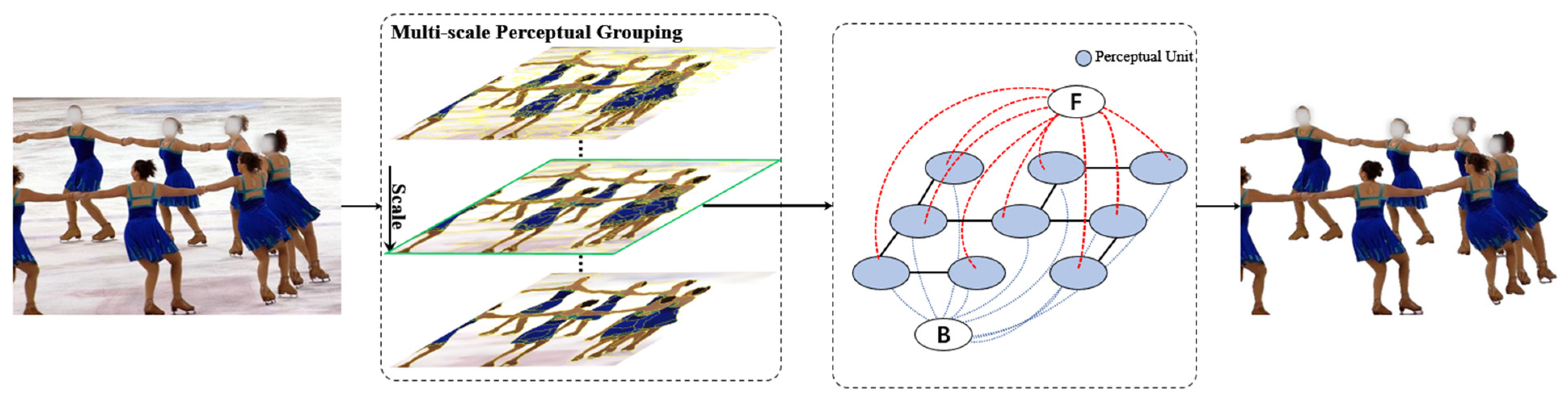
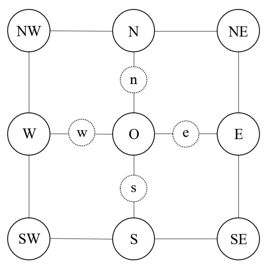
The human eyes observe an image through perceptual units instead of discrete pixels at a proper scale, which enables them quickly to extract the foreground of an image. Inspired by this characteristic, we present a novel image-segmentation model based on multiscale perceptual grouping. The proposed model combines multiscale perceptual grouping and unit-based graph-cut segmentation. In the multiscale perceptual grouping part, a novel total variation regularization is presented to obtain the smoothed image with different scales. At each scale, the pixels of the image are grouped into perceptual units, and the number of perceptual units is utilized to find the proper scale. In the unit-based graph-cut part, the perceptual units are regarded as the nodes in the graph, and a minimum-cut/maximum-flow algorithm is used to split the perceptual units into the foreground and the background. The process is shown in Figure 2.
Given an image , is smoothed and divided into multiple perceptual units. After the image is smoothed to a proper scale, the perceptual units are divided into foreground and background through user interaction. The indicator of whether a unit belongs to the background or foreground is represented as an array of variables , where , with 0 for the background and 1 for the foreground. A unit-based segmentation algorithm can be formulated as the minimization problem of the following energy functional:
where is the appearance term that is used to evaluate the probability that the perceptual units belong to the foreground or the background, represents the parameters of the appearance term, and is the boundary term that represents the similarity between neighboring perceptual units. The details of constructing the above terms are described in the rest of this section.
3.1. Multiscale Perceptual Grouping
When the human eyes group an image into perceptual units, the result is sensitive to the scale of the image. For example, at a fine scale, small regions surrounded by pseudo-edges may be mistaken for perceptual units; at a coarse scale, the adjacent semantic regions may be mistaken for an integrated perceptual unit. In order to eliminate the negative effects at fine scales and preserve the contours between semantic parts, an improved smoothing method is proposed in this paper. The smoothing method is based on the total variation regularization [25], which can be formulated as the following minimization problem:
where denotes the gradients of the smoothed image, and is the weight that is used for the trade-off between the preserved edge and the smoothed region. To remove the inhomogeneity and preserve edge, a new total variation regularization is defined as follows:
where is a constant used to control the edge smoothing. If Equation (2) has a minimum solution, it formally satisfies the Euler–Lagrange equation [26]:
Equation (4) can be simplified as follows:
where
Inspired by the lagged-diffusivity fixed-point iteration algorithm [26], can be iteratively updated to as follows:
where the former is used to preserve the edge, and the latter is used to remove the inhomogeneity. For the latter, when the pixels and are located in a region—that is, —then the value of is large, and is the weighted sum of its neighboring pixels. In this case, the region inhomogeneity is smeared. If pixel lies in one region and in another region, i.e., , then the value of is small, and the is mainly dependent on . In this case, the edges are persevered. In this work, is set as 0.5 according to the edge detection operators. During the iteration process, the smoothing scale increases with the number of iterations. The inhomogeneity is smoothed step by step, and the edges are preserved.
To simulate the human eye’s perception of color changes of the image, the watershed method [27] is utilized to group the perceptual units. The grouping of the perceptual units depends on the scale of the image. For example, in the extreme, the image will be regarded as a single perceptual unit if it is smoothed infinite times. With the increase in the smoothing scale, the number of perceptual units will usually decrease. In this paper, the number of perceptual units is used to find proper scale of the image. The proper scale is considered as the scale where the number of perceptual units does not change significantly with the next scale.
If represents the perceptual units at the smoothing scale , and represents the perceptual units at the smoothing scale , the difference between them is defined as follows:
where is the cardinality of a non-empty set.
If the difference between two adjacent scales is less than the threshold , the smoothing progress is stopped:
The process of multiscale perceptual grouping is shown in Algorithm 1.
| Algorithm 1: Require: the initial image and the threshold . |
| 1: Initialize and . |
| 2. Divide the image into perceptual units by using the watershed method [27]. |
| 3: Compute the smoothed image using Equation (7). |
| 4: Divide the smoothed image into perceptual units by using the watershed method [27]. |
| 5: If the larger than , go back to Step 3. |
| 6. Output the perceptual units . |
3.2. Perceptual-Unit-Based Graph-Cut Method
Since each perceptual unit has approximately homogeneous color, its color distributions can be represented as a Gaussian distribution, as shown in Equation (10):
where and are the mean vector and covariance matrix of color distributions for the perceptual unit , respectively.
The appearance models of the foreground and the background can be constructed as Gaussian mixture models (GMMs) by using the perceptual units. However, regions with similar color distributions may be segmented into different perceptual units because they are not adjacent. These units with similar color distribution should be combined to build more accurate appearance models. Therefore, perceptual units are combined if they satisfy the following condition:
where is the 2-norm operator, and is the threshold of the combination.
After combination, the GMM of the foreground and background can be constructed. The parameters of the two models can be defined as follows:
where and denote the number of combined units in the foreground and background, respectively, and is the ratio of the number of pixels in the combined unit of the foreground and background.
After obtaining the appearance models, a solution to Equation (1) can be optimized via the graph-cut method. However, in this paper, we regard perceptual units as the nodes of the graph, instead of pixels. Therefore, the appearance and boundary terms cannot be simply calculated through the color of the pixels. Due to the perceptual units being represented by Gaussian distributions, KL divergence is used to measure the relationship between them. The KL divergence between two Gaussian distributions can be calculated as follows:
where is the transpose of the matrix, is the inverse of the matrix, and is the trace of the matrix.
The more similar the two Gaussian distributions, the smaller the value of the KL divergence. Due to the KL divergence being asymmetric, the similarity between Gaussian distributions is calculated as follows:
After determining the similarity measurement between the two Gaussian distributions, the boundary term in Equation (1) can be calculated as follows:
where is the mean of all perceptual unit pairs’ similarity in the image, and the appearance model of the FG and the BG can be calculated as follows:
Finally, the perceptual units are divided into foreground and background by using the minimum-cut/maximum-flow algorithm. Compared with GrabCut, the proposed method uses perceptual units instead of discrete pixels, improving the accuracy of estimation of appearance and boundary terms. The whole process of perceptual-unit-based graph-cut method is shown in Algorithm 2.
| Algorithm 2: Require: and using bounding box , the perceptual units s, and the threshold of combination . |
| 1: Initialize x. |
| 2: Construct each perceptual unit as a Gaussian distribution. |
| 3: Compute the term using Equation (15). |
| 4: Estimate the number of background and foreground regions by combining s with the threshold . |
| 5: Estimate the initial using EM. |
| 6: N = 1 |
| 7: For N ≤ 5: |
| 8: Update , given the current using the graph cut. |
| 9: Update , given the current using EM |
| 10: Compute the term using Equation (17) for s. |
| 11: End. |
| 12: Output the foreground . |
4. Numerical Experiments
The experiments were conducted using Visual Studio 2019 on a PC with an Intel-Core i5-10400 CPU @ 2.90 GHz and 16 GB of RAM. The tested images were from the CMU-Cornell iCoseg database [28], which contains 643 images and a mask of ground truth. The precision, recall, intersection over union (IOU) [29], and F-measure [30] metrics were used to evaluate the performance of the results. The precision and recall are defined as follows:
where and are the extracted foreground and the ground truth, respectively.
4.1. Parameter Discussion
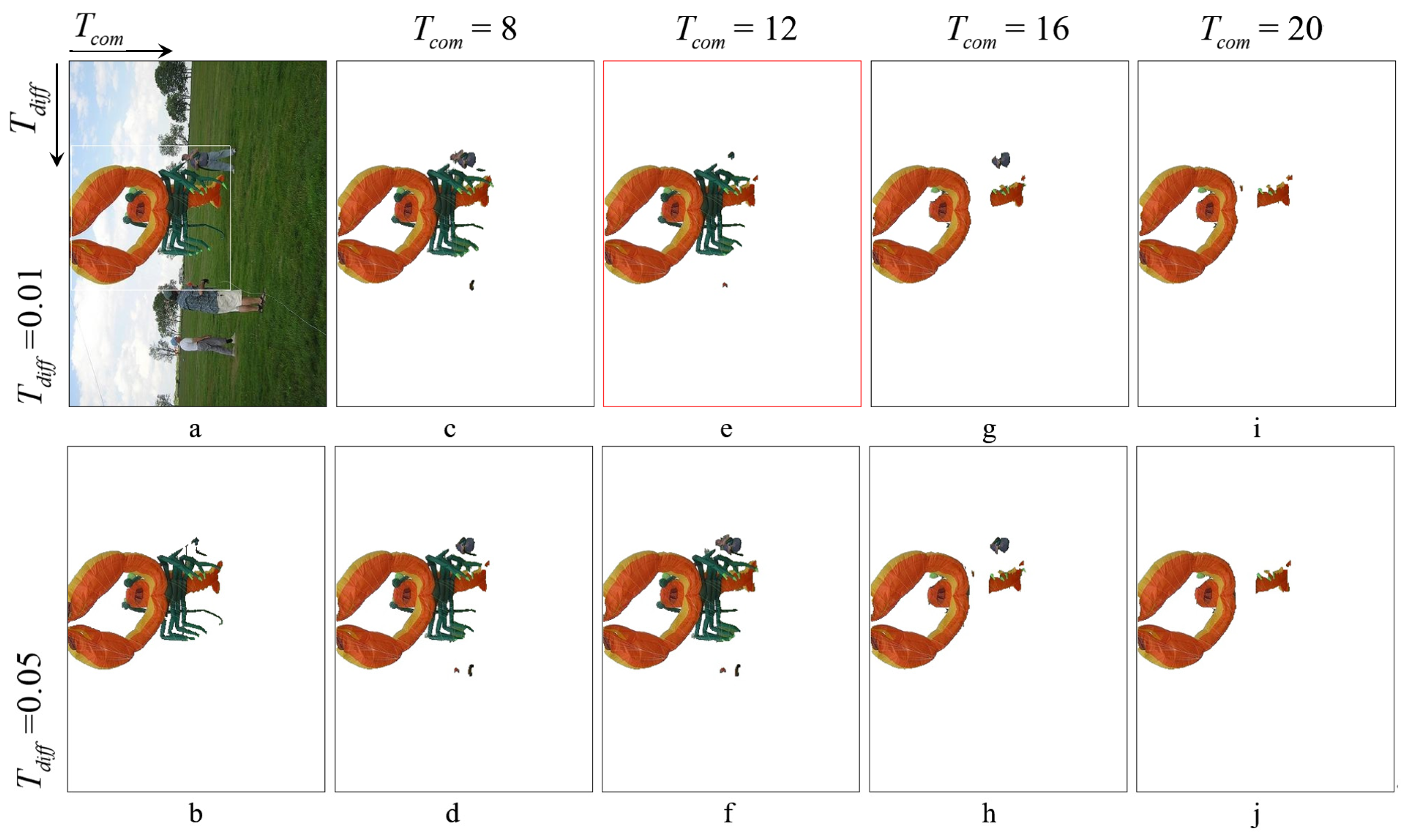
The segmentation results are influenced by the scale of the image and the appearance model in the unit-based graph-cut method. Therefore, two parameters are discussed: the first is in Equation (7), and the second is in Equation (11). controls the scale of smoothness, which affects the segmentation of the perceptual units. If is too large, the smoothing process will stop prematurely; if is too small, the image may be over-smoothed. is used to determine the combination of perceptual units in the image, which will affect the accuracy of the appearance model. In one extreme, if , the perceptual units will not be combined, and the number of Gaussian distributions will be large in the GMMs. In another case, if , the image will be represented as a single Gaussian distribution.
The experiments with different parameters were conducted on the CMU-Cornell iCoseg database. Some of the results are shown in Figure 3. When , the image is under-smoothed, and the small regions are mistakenly segmented into the foreground, as shown in Figure 3f. When , the performance results become better due to the sufficient smoothness of the image, as shown in Figure 3e. When is small, the perceptual units may not be combined to form a unified Gaussian distribution, which leads to an excessive number of Gaussian distributions in the GMMs. When is large, the situation is the opposite. Both inaccurate GMMs will result in poor performance of segmentation, as shown in Figure 3c,g, respectively. Therefore, in this paper, we set as 0.01 and as 12.
4.2. Comparison and Analysis
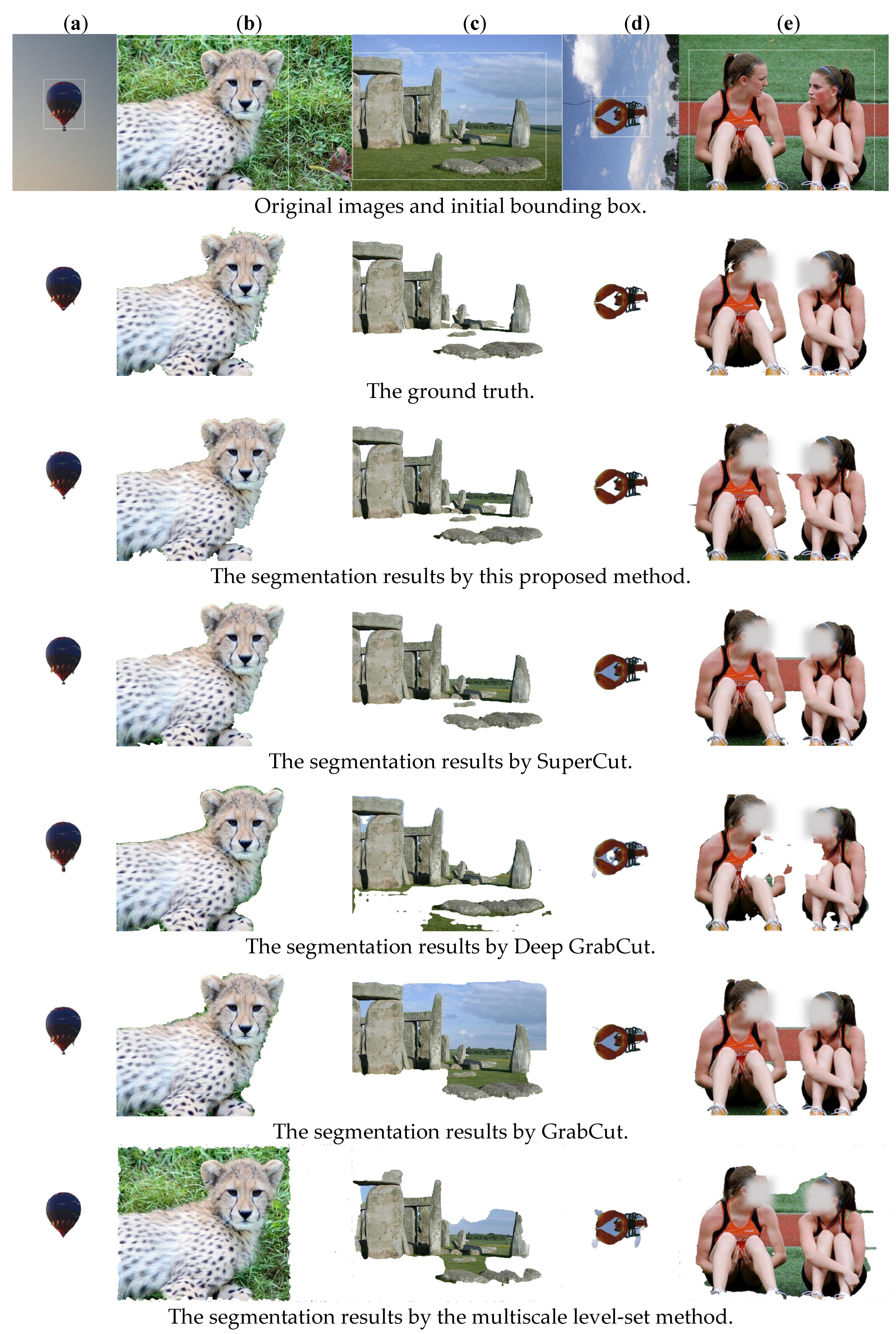
In order to show the performance of the proposed method, experiments were conducted on the CMU-Cornell iCoseg database by comparing it with four other methods. These four methods included the multiscale level-set model [7], GrabCut [23], SuperCut [24], and Deep GrabCut [11]. The segmentation metrics are detailed in Table 1, which shows that the proposed method is superior to other methods.
Five representative segmentation results are shown in Figure 4. Figure 4a shows an image with a homogeneous background and foreground. Figure 4b has a background with many edges. In Figure 4c, the scene contains sky, grass, and stones, making it a complicated image. Figure 4d shows an image with a hole-like background in the foreground. Figure 4e has two objects in the foreground. For the simple images, all of the methods show satisfactory results, as in Figure 4a. For the complex images, the proposed method has better segmentation performance than the other methods.
The proposed method combines multiscale perceptual grouping and unit-based graph-cut segmentation. In the multiscale perceptual grouping, the image is smoothed to a proper scale and divided into perceptual units, eliminating the inhomogeneity and preserving the edges. In the unit-based segmentation part, the perceptual units are modeled by Gaussian distributions. KL divergence is employed to measure the relationship between Gaussian distributions. Then, the appearance models of the foreground and background are represented as GMMs by combining the perceptual units. Compared with GrabCut, the proposed method helps to find the optimal number of Gaussian distributions in the GMMs, and improves the accuracy of parameter estimation. After that, a graph is constructed from the perceptual units instead of the pixels, which improves the global accuracy of segmentation. Finally, the foreground is segmented by using the minimum-cut/maximum-flow algorithm. Both of the parts facilitated improved segmentation performance, as shown in Figure 4d,e.
The performance of the multiscale level-set model [7] is poor for the complex images, as shown in Figure 4b. The reason for this is that even if the multiscale level set removes the inhomogeneity of the image, it still cannot avoid the local optima of the segmentation function. The background of Figure 4b is composed of weeds with many edges, which makes it easy for the algorithm to stay at the local optimum, producing bad results.
The SuperCut [24] method uses SLIC to segment the image into superpixels for constructing the appearance model. After that, the foreground is extracted at the pixel level. Compared to SuperCut, the appearance models in the proposed method are constructed by perceptual units with irregular size, instead of by superpixels with fixed sizes. Moreover, the proposed method segments the foreground using the perceptual units instead of pixels. SuperCut achieves good performance for the details, since it uses pixel-level segmentation. However, for the image with the hole-like background that appears in the foreground, the segmentation results of the proposed method have a better performance, as shown in Figure 3d.
Deep GrabCut [11] employs an encoder–decoder structure network, which is trained end-to-end on the PASCAL 2012 database. Deep learning methods, including Deep GrabCut, have a common problem—they achieve good performance for the classes that appear in the training set, as shown in Figure 3b; however, the segmentation performance is poor for the new objects, such as Figure 3d. Another drawback of Deep GrabCut is that there are discrete pixels that are incorrectly segmented in the results, such as in Figure 3c. In addition, when multiple objects appear in the initial box, the segmentation performance is also unsatisfactory.
The segmentation metrics and computational cost for the image in Figure 3 are listed in Table 2. For the simple images, the IOU and F-measures are similar for all of the methods. For the complex images, the metrics of the proposed method are obviously better than those of other methods. However, the computational cost is relatively higher than that of the other methods. The reason for this is that the multiscale perceptual grouping is an iterative process, and the computational cost depends on the inhomogeneity of the images.
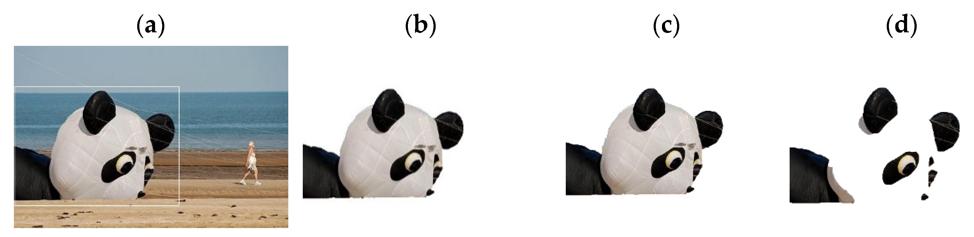
Even though the overall performance of the proposed method is better than that of the other methods, it may achieve poor results when there are similar color regions in the foreground and background. The reason for this is that the segmentation of the proposed method is based on perceptual regions instead of pixels. When the maximum-flow/minimum-cut algorithm is executed, the entire perceptual unit may be removed from the foreground as a whole, such as the panda head in Figure 5.
5. Conclusions
In this work, we propose a multiscale perceptual grouping segmentation model. The proposed model extends the graph-cut method in two aspects: (1) a novel total variation regularization is designed, which smooths the image into different scales to remove inhomogeneity and preserve edges; (2) perceptual units are used instead of discrete pixels in the graph-cut method, improving the accuracy of parameter estimation. Experiments on the CMU-Cornell iCoseg database show that the proposed model achieves a good performance. However, the measurement of similarity between Gaussian distributions has a disadvantage, because KL divergence is only meaningful for distributions with overlap. In the future, we plan to explore a new method to measure the similarity between Gaussian distributions.
Author Contributions
Conceptualization, B.F. and K.H.; Data Curation, B.F.; Formal Analysis, B.F.; Investigation, B.F.; Methodology, B.F. and K.H.; Project Administration, K.H.; Resources, B.F.; Supervision, K.H.; Validation, B.F. and K.H.; Visualization, B.F.; Writing—Original Draft, B.F.; Writing—Review and Editing, B.F. and K.H. All authors have read and agreed to the published version of the manuscript.
Funding
This research was funded by the National Key Research and Development Program of China (grant number: 2018YFC0832301).
Conflicts of Interest
The authors declare no conflict of interest.
Appendix A
Given Equation (4):
Figure A1.
A target pixel and its adjacent pixels. denote the four adjacent pixels, while denote the four midway points, which are not directly available from the digital image.
Figure A1.
A target pixel and its adjacent pixels. denote the four adjacent pixels, while denote the four midway points, which are not directly available from the digital image.

The finite difference scheme is used to calculate the smoothed image. Let be a member of the adjacent pixel set and the corresponding midway points, as shown in Figure 4.
The term in Equation (A1) is simply written as .
If , then the divergence term is firstly discretized by central differencing:
Next, we generate approximations at the midway point. Take for example:
where:
A similar calculation applies to the other three midway points , and . After that, Equation (A2) can be calculated as follows:
If and , Equation (A5) can be simplified as follows:
After obtaining Equation (A6), Equation (A1) can be simplified as follows:
where:
References
- Wang, L.; Chen, G.; Shi, D.; Chang, Y.; Chan, S.; Pu, J.; Yang, X. Active contours driven by edge entropy fitting energy for image segmentation. Signal Process. 2018, 149, 27–35. [Google Scholar] [CrossRef] [PubMed]
- Li, M.; Wang, L.; Deng, S.; Zhou, C. Color image segmentation using adaptive hierarchical-histogram thresholding. PLoS ONE 2020, 15, e0226345. [Google Scholar] [CrossRef] [PubMed]
- Tong, J.; Zhao, Y.; Zhang, P.; Chen, L.; Jiang, L. MRI brain tumor segmentation based on texture features and kernel sparse coding. Biomed. Signal Process. Control 2019, 47, 387–392. [Google Scholar] [CrossRef]
- Long, J.; Shelhamer, E.; Darrell, T. Fully convolutional networks for semantic segmentation. In Proceedings of the IEEE conference on computer vision and pattern recognition, Boston, MA, USA, 7–12 June 2015; pp. 3431–3440. [Google Scholar]
- Chen, L.C.; Papandreou, G.; Kokkinos, I.; Murphy, K.; Yuille, A.L. Deeplab: Semantic image segmentation with deep convolutional nets, atrous convolution, and fully connected crfs. IEEE Trans. Pattern Anal. Mach. Intell. 2017, 40, 834–848. [Google Scholar] [CrossRef] [Green Version]
- Minaee, S.; Boykov, Y.Y.; Porikli, F.; Plaza, A.J.; Kehtarnavaz, N.; Terzopoulos, D. Image segmentation using deep learning: A survey. arXiv 2021, arXiv:2001.05566. [Google Scholar] [CrossRef]
- Li, Y.; Feng, X. A multiscale image segmentation method. Pattern Recognit. 2016, 52, 332–345. [Google Scholar] [CrossRef]
- Tang, M.; Gorelick, L.; Veksler, O.; Boykov, Y. GrabCut in One Cut. In Proceedings of the 2013 IEEE International Conference on Computer Vision (ICCV 2013), Sydney, Australia, 1–8 December 2013; pp. 1769–17761. [Google Scholar] [CrossRef]
- Tunga, P.P.; Singh, V. Extraction and description of tumour region from the brain MRI image using segmentation techniques. In Proceedings of the 2016 IEEE International Conference on Recent Trends in Electronics, Information & Communication Technology (RTEICT), Bangalore, India, 20–21 May 2016; pp. 1571–1576. [Google Scholar]
- Kumar, S.; Pant, M.; Kumar, M.; Dutt, A. Colour image segmentation with histogram and homogeneity histogram difference using evolutionary algorithms. Int. J. Mach. Learn. Cybern. 2018, 9, 163–183. [Google Scholar] [CrossRef]
- Xu, N.; Price, B.; Cohen, S.; Yang, J.; Huang, T. Deep grabcut for object selection. arXiv 2017, arXiv:1707.00243. [Google Scholar]
- Grady, L. Random walks for image segmentation. IEEE Trans. Pattern Anal. Mach. Intell. 2006, 28, 1768–1783. [Google Scholar] [CrossRef] [Green Version]
- Tsai, A.; Yezzi, A.; Willsky, A.S. Curve evolution implementation of the Mumford-Shah functional for image segmentation, denoising, interpolation, and magnification. IEEE Trans. Image Process. 2001, 10, 1169–1186. [Google Scholar] [CrossRef] [Green Version]
- Boykov, Y.Y.; Jolly, M.P. Interactive graph cuts for optimal boundary & region segmentation of objects in ND images. In Proceedings of the eighth IEEE international conference on computer vision, ICCV 2001, Vancouver, BC, Canada, 7–14 July 2001; Volume 1, pp. 105–112. [Google Scholar]
- Lu, Y.; Chen, Y.; Zhao, D.; Chen, J. Graph-FCN for image semantic segmentation. In International Symposium on Neural Networks; Springer: Cham, Switzerland, 2019; pp. 97–105. [Google Scholar]
- Jesson, A.; Arbel, T. Brain tumor segmentation using a 3D FCN with multi-scale loss. In International MICCAI Brainlesion Workshop; Springer: Cham, Switzerland, 2017; pp. 392–402. [Google Scholar]
- Villa, M.; Dardenne, G.; Nasan, M.; Letissier, H.; Hamitouche, C.; Stindel, E. FCN-based approach for the automatic segmentation of bone surfaces in ultrasound images. Int. J. Comput. Assist. Radiol. Surg. 2018, 13, 1707–1716. [Google Scholar] [CrossRef] [PubMed]
- Tang, W.; Zou, D.; Yang, S.; Shi, J.; Dan, J.; Song, G. A two-stage approach for automatic liver segmentation with Faster R-CNN and DeepLab. Neural Comput. Appl. 2020, 32, 6769–6778. [Google Scholar] [CrossRef]
- Yeo, S.Y.; Xie, X.; Sazonov, I.; Nithiarasu, P. Segmentation of biomedical images using active contour model with robust image feature and shape prior. Int. J. Numer. Methods Biomed. Eng. 2014, 30, 232–248. [Google Scholar] [CrossRef] [Green Version]
- Chan, T.F.; Vese, L.A. Active contours without edges. IEEE Trans. Image Process. 2001, 10, 266–277. [Google Scholar] [CrossRef] [Green Version]
- Peng, Y.; Liu, F.; Liu, S. Active contours driven by normalized local image fitting energy. Concurr. Comput. Pract. Exp. 2014, 26, 1200–1214. [Google Scholar] [CrossRef]
- Miao, J.; Huang, T.Z.; Zhou, X.; Wang, Y.; Liu, J. Image segmentation based on an active contour model of partial image restoration with local cosine fitting energy. Inf. Sci. 2018, 447, 52–71. [Google Scholar] [CrossRef]
- Rother, C.; Kolmogorov, V.; Blake, A. “GrabCut” interactive foreground extraction using iterated graph cuts. ACM Trans. Graph. TOG 2004, 23, 309–314. [Google Scholar] [CrossRef]
- Wu, S.; Nakao, M.; Matsuda, T. SuperCut: Superpixel based foreground extraction with loose bounding boxes in one cutting. IEEE Signal Process. Lett. 2017, 24, 1803–1807. [Google Scholar] [CrossRef]
- Chan, T.F.; Osher, S.; Shen, J.H. The Digital TV Filter and Nonlinear Denoising. IEEE Trans. Image Process. 2001, 10, 231–241. [Google Scholar] [CrossRef] [Green Version]
- Antman, S.S.; Marsden, J.E.; Sirovich, L. Mathematical Problems in Image Processing: Partical Differential Equations and the Calculus of Variations; Springer Science Business Media, LLC: Berlin/Heidelberg, Germany, 2006; pp. 70–72. [Google Scholar]
- Vincent, L.; Soille, P. Watersheds in digital spaces: An efficient algorithm based on immersion simulations. IEEE Trans. Pattern Anal. Mach. Intell. 1991, 13, 583–598. [Google Scholar] [CrossRef] [Green Version]
- Batra, D.; Kowdle, A.; Parikh, D.; Luo, J.; Chen, T. icoseg: Interactive co-segmentation with intelligent scribble guidance. In Proceedings of the 2010 IEEE computer society conference on computer vision and pattern recognition, San Francisco, CA, USA, 13–18 June 2010; pp. 3169–3176. [Google Scholar]
- Pont-Tuset, P.; Marques, F. Supervised Evaluation of Image Segmentation and Object Proposal Techniques. IEEE Trans. Pattern Anal. Mach. Intell. 2016, 38, 1465–1478. [Google Scholar] [CrossRef] [PubMed] [Green Version]
- Van Rijsbergen, C. Information retrieval: Theory and practice. In Proceedings of the Joint IBM/University of Newcastle upon Tyne Seminar on Data Base Systems, Newcastle upon Tyne, UK, 4–7 September 1979; pp. 1–14. [Google Scholar]
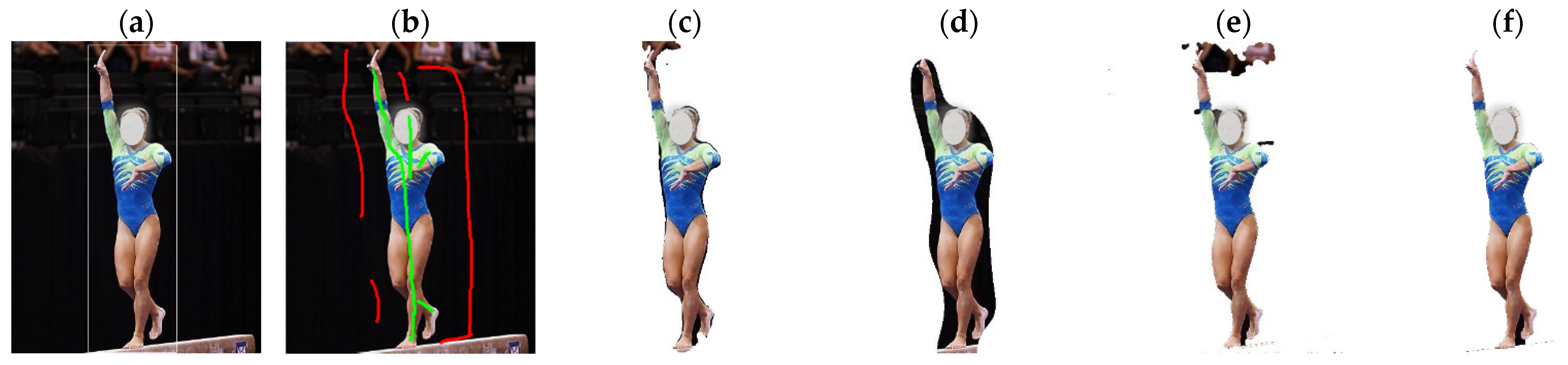
Figure 1.
Segmentation results of representative segmentation methods: (a) is the image with a bounding box, which is the user interaction for (c,e,f). (b) is the initial user interaction for (d). (c–f) show the segmentation results of Deep GrabCut [11], the random walk method [12], the level-set method [13], and the graph-cut method [14], respectively.

Figure 2.
Overview of the proposed segmentation framework: Given an image, the perceptual units are obtained via the multiscale perceptual grouping method. After that, a graph is constructed by using the perceptual units, and the foreground is segmented.
Figure 2.
Overview of the proposed segmentation framework: Given an image, the perceptual units are obtained via the multiscale perceptual grouping method. After that, a graph is constructed by using the perceptual units, and the foreground is segmented.

Figure 3.
The segmentation performance with different parameters: (a) The original image and the initial boundary box, (b) the ground truth, (c–j) the segmented results with at 8, 12, 16, and 20, and at 0.01 and 0.05.
Figure 3.
The segmentation performance with different parameters: (a) The original image and the initial boundary box, (b) the ground truth, (c–j) the segmented results with at 8, 12, 16, and 20, and at 0.01 and 0.05.

Figure 4.
Comparison of the proposed method with GrabCut, SuperCut, Deep GrabCut, and the multiscale level-set method on the partial images in CMU-Cornell iCoseg database. (a–e) are the balloon, leopard, stone, kite and humans, respectively.
Figure 4.
Comparison of the proposed method with GrabCut, SuperCut, Deep GrabCut, and the multiscale level-set method on the partial images in CMU-Cornell iCoseg database. (a–e) are the balloon, leopard, stone, kite and humans, respectively.

Figure 5.
A poor result of the proposed method. (a) the original image with bounding box; (b) ground truth (c) result of GrabCut (d) result of the proposed method.
Figure 5.
A poor result of the proposed method. (a) the original image with bounding box; (b) ground truth (c) result of GrabCut (d) result of the proposed method.


Table 1.
Segmentation metrics for the CMU-Cornell iCoseg database.
| Methods | IOU | F-Measure | ||||
|---|---|---|---|---|---|---|
| Min | Mean | Max | Min | Mean | Max | |
| The CMU-Cornell iCoseg database | ||||||
| This method | 0.328 | 0.790 | 0.995 | 0.579 | 0.882 | 0.997 |
| SuperCut [24] | 0.253 | 0.764 | 0.994 | 0.540 | 0.841 | 0.997 |
| Deep GrabCut [11] | 0.254 | 0.752 | 0.984 | 0.537 | 0.836 | 0.992 |
| GrabCut [23] | 0.221 | 0.763 | 0.996 | 0.525 | 0.841 | 0.998 |
| Multiscale level-set method [7] | 0.0 | 0.599 | 0.975 | 0.200 | 0.725 | 0.987 |
Table 2.
Segmentation metrics and the computational cost re: Figure 4.
Table 2.
Segmentation metrics and the computational cost re: Figure 4.
| Methods | Figure 3a | Figure 3b | Figure 3c | Figure 3d | Figure 3e |
|---|---|---|---|---|---|
| 332 × 500 | 500 × 332 | 500 × 372 | 500 × 372 | 500 × 372 | |
| This method | |||||
| Precision | 0.966 | 0.995 | 0.930 | 0.959 | 0.936 |
| Recall | 0.993 | 0.965 | 0.984 | 0.981 | 0.991 |
| F-measure | 0.979 | 0.980 | 0.957 | 0.970 | 0.963 |
| IOU | 0.959 | 0.960 | 0.917 | 0.941 | 0.928 |
| Computational cost(s) | 2.138 | 12.39 | 12.68 | 10.35 | 13.80 |
| SuperCut [24] | |||||
| Precision | 0.974 | 0.986 | 0.919 | 0.830 | 0.917 |
| Recall | 0.998 | 0.972 | 0.978 | 0.983 | 0.989 |
| F-measure | 0.986 | 0.979 | 0.947 | 0.900 | 0.952 |
| IOU | 0.972 | 0.959 | 0.899 | 0.818 | 0.908 |
| Computational cost(s) | 4.950 | 9.442 | 12.29 | 5.665 | 9.609 |
| Deep GrabCut [11] | |||||
| Precision | 0.927 | 0.963 | 0.830 | 0.779 | 0.969 |
| Recall | 0.999 | 0.995 | 0.968 | 0.991 | 0.848 |
| F-measure | 0.961 | 0.979 | 0.894 | 0.872 | 0.904 |
| IOU | 0.926 | 0.958 | 0.808 | 0.773 | 0.825 |
| Computational cost(s) | 3.215 | 3.175 | 3.501 | 3.447 | 2.993 |
| GrabCut [23] | |||||
| Precision | 0.968 | 0.962 | 0.506 | 0.813 | 0.911 |
| Recall | 0.999 | 0.988 | 0.991 | 0.992 | 0.994 |
| F-measure | 0.978 | 0.975 | 0.670 | 0.894 | 0.951 |
| IOU | 0.959 | 0.951 | 0.504 | 0.808 | 0.907 |
| Computational cost(s) | 3.610 | 8.001 | 10.94 | 4.279 | 8.359 |
| The multiscale level-set method [7] | |||||
| Precision | 0.993 | 0.611 | 0.750 | 0.693 | 0.812 |
| Recall | 0.973 | 0.976 | 0.844 | 0.949 | 0.956 |
| F-measure | 0.983 | 0.752 | 0.794 | 0.801 | 0.878 |
| IOU | 0.966 | 0.602 | 0.659 | 0.668 | 0.783 |
| Computational cost(s) | 4.116 | 2.106 | 7.132 | 7.250 | 7.074 |
Publisher’s Note: MDPI stays neutral with regard to jurisdictional claims in published maps and institutional affiliations. |
© 2022 by the authors. Licensee MDPI, Basel, Switzerland. This article is an open access article distributed under the terms and conditions of the Creative Commons Attribution (CC BY) license (https://creativecommons.org/licenses/by/4.0/).
Share and Cite
MDPI and ACS Style
Feng, B.; He, K. Image Segmentation via Multiscale Perceptual Grouping. Symmetry 2022, 14, 1076. https://0-doi-org.brum.beds.ac.uk/10.3390/sym14061076
AMA Style
Feng B, He K. Image Segmentation via Multiscale Perceptual Grouping. Symmetry. 2022; 14(6):1076. https://0-doi-org.brum.beds.ac.uk/10.3390/sym14061076
Chicago/Turabian StyleFeng, Ben, and Kun He. 2022. "Image Segmentation via Multiscale Perceptual Grouping" Symmetry 14, no. 6: 1076. https://0-doi-org.brum.beds.ac.uk/10.3390/sym14061076
Note that from the first issue of 2016, this journal uses article numbers instead of page numbers. See further details here.