Identification of Material Properties of Elastic Plate Using Guided Waves Based on the Matrix Pencil Method and Laser Doppler Vibrometry

Abstract

Ultrasonic based inspection of thin-walled structures often requires prior knowledge of their mechanical properties. Their accurate estimation could be achieved in a non-destructive manner employing, e.g., elastic guided waves. Such procedures require efficient approaches for experimental data extraction and processing, which is still a challenging task. An advanced automated technique for material properties identification of an elastic waveguide is proposed in this investigation. It relies on the information on dispersion characteristics of guided waves, which are extracted by applying the matrix pencil method to the measurements obtained via laser Doppler vibrometry. Two objective functions have been successfully tested, and the advantages of both approaches are discussed (accuracy vs. computational costs). The numerical analysis employing the synthetic data generated via the mathematical model as well as experimental data shows that both approaches are stable and accurate. The influence of the presence of various modes in the extracted data is investigated. One can conclude that the influence of the corruptions related to the extraction of dispersion curves is not critical if the majority of guided waves propagating in the considered frequency range are presented. Possible extensions of the proposed technique for damaged and multi-layered structures are also discussed.

1. Introduction

Information about mechanical properties of engineering structures is essential equally at the stage of their manufacturing (e.g., for their quality control) as well as at the operation stage (e.g., for the periodic structural integrity assessment). Besides, prior accurate knowledge of material properties is a crucial point for computational models employed at various stages of the structural design, since discrepancies between assumed and actual values of such parameters may cause large errors in the prediction, resulting in miscellaneous undesired consequences. Numerous static or dynamic methods are being developed for accurate evaluation of the material elastic constants [1,2,3]. The former include tensile, compression, and bending tests, whereas the latter typically rely on low-frequency vibration or high-frequency ultrasonic-related approaches.

Recent advancements in experimental facilities and devices caused the intensive development of non-destructive dynamic approaches for material characterization. Detailed reviews of the vibrational evaluation methods, where low frequencies are employed, can be found in [3,4]. Identification techniques based on ultrasonic guided waves (GW) rely on GW propagation characteristics, which carry information on the material properties in a wider frequency range compared with vibrational methods. Therefore, they require multi-modal high-resolution signals, where data collection and extraction of multiple propagating modes are necessary, which is still a challenging task [5]. Typically, scanning of a certain area of the specimen surface is needed to obtain dispersion properties, and, therefore, various experimental techniques are used. Chen et al. [5], Okumura et al. [6,7], Bochud et al. [8] and many others used a linear array probe attached at the surface of a specimen for dispersion data extraction. Since the attachment of an ultrasonic probe changes the guiding properties of the waveguide in the area of contact, non-contact techniques are preferable. Among them, laser-based approaches are becoming widespread: GWs are excited by a laser source through thermoelastic conversion [9] or by a piezoelectric transducer [10,11,12], and surface displacement/velocity is detected by laser interferometry. A scanning procedure can also be performed by an air-coupled transducer, e.g., Takahashi et al. [13] varied angle of incidence, in order to estimate the properties of a bi-layered structure. In addition, the non-contact technique based on the transient grating method was employed for the identification of elastic properties of a composite consisting of GaN nanowires embedded into a dielectric matrix [14].

Waveguide mechanical properties are usually obtained via the minimization of the discrepancy between the measured and calculated wave characteristics. Therefore, an optimization problem is to be solved, where an objective function providing a stable numerical procedure fitting a waveguide model to the experimental data should be constructed. In vibrational-based material identification, the objective function can generally be defined in various forms involving natural frequencies and mode shapes [4]. For instance, Pagnotta and Stigliano [15] investigated the feasibility of a vibration-based approach using natural frequencies of thin isotropic plates of various shapes to determine Young’s modulus, Poisson’s ratio, mass density and thickness, showed the robustness of the identification process with respect to measurement noise. Within GW-based approaches, as soon as measurements are made, the corresponding GW characteristic features (e.g., wavenumbers, phase or group velocities or slownesses) are to be accurately extracted from the experimental data. For this purpose, the two-dimensional Fourier transform [8,10,14,16], the dynamic mode decomposition [17] or the matrix pencil method (MPM) [18,19,20] are employed.

The specific features of GWs obtained from the experiment are further used for the inverse problem solution, which also involves intensive computations using mathematical models [8,14,20,21]. In GW-based identification methods, various objective functions are constructed employing dispersion characteristics. A typical approach is to consider the discrepancy between experimental and theoretical dispersion properties of GWs [11,13]. Its minimization demands calculation of dispersion curves of a waveguide at each step. The latter is reduced to root-finding procedures, which are cumbersome for multi-layered waveguides. Besides, reliable mode separation and reconstruction methods allowing for individual mode extraction from dispersive multi-modal GW signals are needed [22]. Fairuschin et al. [23] used an alternative method, in which the dispersion properties are calculated by solving the underlying differential equations using the spectral collocation method. The latter provides a good trade-off between precision, implementation effort, and computation, but it is not always robust [24]. It should be mentioned that additional features of GWs such as zero group velocities can be combined with waveguide modelling for material properties identification [25]. Alternative approaches to avoiding root-finding procedures, which are time-consuming, rely also on dispersion characteristics. Thelen et al. [21] proposed a thorough assessment of the effective mechanical behaviour of pSi using dispersion maps, where the maps are obtained by converting the modelled guided modes into a binary image. The objective function is defined as the mean value of the element-wise product between experimental and modelled dispersion maps. Chen et al. [5] and Bochud et al. [8] defined the objective function as the ratio of the number of experimental pairs wavenumber-frequency estimates satisfying the dispersion equation to the number of the total estimates for an isotropic layer. In this case, roots of the dispersion equation are not necessary, since the experimental wavenumber-frequency is substituted into the dispersion equation, and the objective function is defined using the signum function, showing sign change in the vicinity of a certain wavenumber at a given frequency, for more details see [5,8]. Also, Green’s matrices can be employed instead of the dispersion equation [14], which demands more computational time (2–3 times), but provides a smoother objective function.

In this paper, a novel automated technique for the identification of material properties of an elastic waveguide is proposed, validated and verified using synthesized and experimental data. The approach relies on the information on the dispersion characteristics of GWs, which are extracted here by applying the MPM to the measurements obtained via laser Doppler vibrometry. Two objective functions have been composed: the first functional uses information on slownesses, while the second one employs the Fourier transform of Green’s matrix [14]. The numerical analysis relying on the synthesized data generated via the mathematical model (the algorithm of data synthesis is described in Section 5) shows that both approaches are stable. With the help of synthesized data, the accuracy of the two approaches is compared and the efficiency and the biasedness of the obtained estimates is tested. It is demonstrated that the approach using slownesses is more accurate, but it is more time-consuming. The influence of the presence of certain modes in the extracted data is also investigated. One can conclude that the influence of the corruptions related to the extraction of dispersion curves extraction is not critical if the majority of guided waves propagating in the considered frequency range are presented. Discussions of the possible extensions of the proposed technique for damaged and multi-layered structures are also given.

2. Theoretical Determination of Guided Waves Characteristics

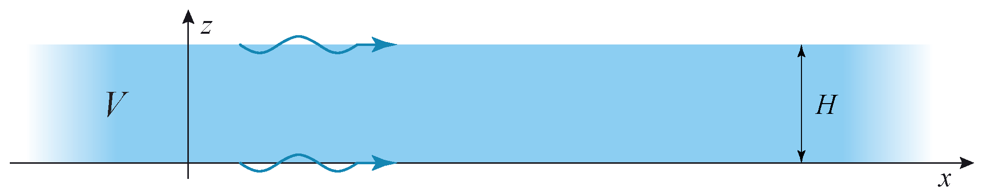
Let us consider the steady-state motion of an elastic layer $V=\left\{\right|x|<\infty ,-H\le z\le 0\}$ of thickness H characterized by the mass density $\rho$, Young’s modulus E, and Poisson’s ratio $\nu$ as shown in Figure 1, so that the parameter of the model $\mathit{\theta }=\{E,\nu ,H\}$ is introduced. The mass density $\rho$ is not included into the model parameter since the dispersion characteristics of the layer depend only three values, and the density can be determined without ultrasonic measurements. For the time-harmonic wave motion with the angular frequency $\omega =2\pi f$, the displacement vector $\mathit{u}$ obeys the symmetric governing equations

$${\displaystyle \frac{1-\nu }{1-2\nu }}\nabla ·\nabla \mathit{u}-{\displaystyle \frac{1}{2}}\nabla \times \left(\nabla \times \mathit{u}\right)+{\displaystyle \frac{(1+\nu )\rho }{E}}{\omega }^2\mathit{u}=\mathbf{0}.$$

(1)

Hooke’s law relates the components of the stress tensor ${\sigma }_{ik}$ and the displacement vector $\mathit{u}$. The upper and lower surfaces of the layer are assumed to be stress-free

$${\sigma }_{i2}(x,0)={\sigma }_{i2}(x,-H)=0,\forall x.$$

(2)

Since the solution corresponding to a guided wave propagating in a positive direction with the wavenumber $\zeta$ at the angular frequency $\omega =2\pi f$ (f is the dimensional frequency) has the form:

$$\mathit{u}(x,z,\omega )=\mathit{U}\left(z\right)exp\left[\mathrm{i}\right(\zeta x-\omega t\left)\right].$$

The latter form is substituted into governing Equation (1), which leads to the following system of ordinary differential equations:

$${\mathbf{B}}_2\left(\zeta \right){\displaystyle \frac{{\mathrm{d}}^2\mathit{U}\left(z\right)}{\mathrm{d}{z}^2}}+{\mathbf{B}}_1\left(\zeta \right){\displaystyle \frac{\mathrm{d}\mathit{U}\left(z\right)}{\mathrm{d}z}}+{\omega }^2{\mathbf{B}}_0\left(\zeta \right)\mathit{U}\left(z\right)=\mathbf{0}.$$

(3)

Differential Equation (3) can be rewritten in the following form

$${\displaystyle \frac{\mathrm{d}\mathit{Y}}{\mathrm{d}z}}=\mathbf{P}(\zeta ,f)\mathit{Y},$$

(4)

$$\mathit{Y}=\left\{U_1,U_2,{\displaystyle \frac{\partial U_1}{\partial z}},{\displaystyle \frac{\partial U_2}{\partial z}}\right\}.$$

The solution of (4) can be written in terms of the matrix $\mathbf{M}(\zeta ,f)$ composed of eigenvectors, $\mathbf{E}(\zeta ,f,z)=\mathrm{diag}\left\{exp\left({\gamma }_{1}z\right),\dots ,exp\left({\gamma }_{4}z\right)\right\}$, where ${\gamma }_1\left(f\right)$ are eigenvalues of $\mathbf{P}(\zeta ,f)$, and the vector of unknown coefficients $\mathit{t}$:

$$\mathit{Y}(\zeta ,f,z)=\mathbf{M}(\zeta ,f)·\mathbf{E}(\zeta ,f,z)·\mathit{t}.$$

(5)

Replacement of (5) into stress-free boundary conditions (2) gives

$$\begin{array}{c}\mathbf{T}\left(\zeta \right)·\mathbf{M}(\zeta ,f)·\mathbf{E}(\zeta ,f,0)·\mathit{t}=\mathbf{0},\\ \mathbf{T}\left(\zeta \right)·\mathbf{M}(\zeta ,f)·\mathbf{E}(\zeta ,f,-H)·\mathit{t}=\mathbf{0},\end{array}$$

which can be rewritten in terms of a four-by-four matrix $\mathbf{D}$

$$\mathbf{D}(\zeta ,f)·\mathit{t}=0$$

(6)

and differential operator $\mathbf{T}\left(\zeta \right)$ corresponding to Hooke’s law. Therefore, the solution ${\zeta }_k\left(f\right)$ of the dispersion relation

$$\Delta (f,{\zeta }_k)=\det \mathbf{D}({\zeta }_k,f)=0$$

(7)

gives wavenumbers of guided waves propagating in the elastic layer. In order to construct components of the Fourier transform of Green’s matrix ${\mathbf{K}}_{ij}(\zeta ,f)$, the right-hand side of the system (6) is substituted by ${\mathit{g}}_j$ (${\mathit{g}}_1={\left\{1,0,0,0\right\}}^{\mathrm{T}}$, ${\mathit{g}}_2={\left\{0,1,0,0\right\}}^{\mathrm{T}}$) assuming that the load is applied at the lower boundary $z=0.$ The latter leads to the following system:

$$\mathbf{D}(\zeta ,f)·{\mathit{t}}_j={\mathit{g}}_j.$$

(8)

The solution of (8) is then substituted into (5), and the Fourier transform of Green’s matrix can be represented as follows

$$\mathit{K}(f,\zeta /f,z,\mathit{\theta })=\mathbf{M}(\zeta ,f)·\mathbf{E}(\zeta ,f,z)·\left\{{\mathit{t}}_1(\zeta ,f),{\mathit{t}}_2(\zeta ,f)\right\}$$

(9)

in terms of slowness value $s\left(\mathit{\theta }\right)=\zeta \left(\mathit{\theta }\right)/f$, which is employed further.

3. Experimental Data Extraction Using the Matrix Pencil Method

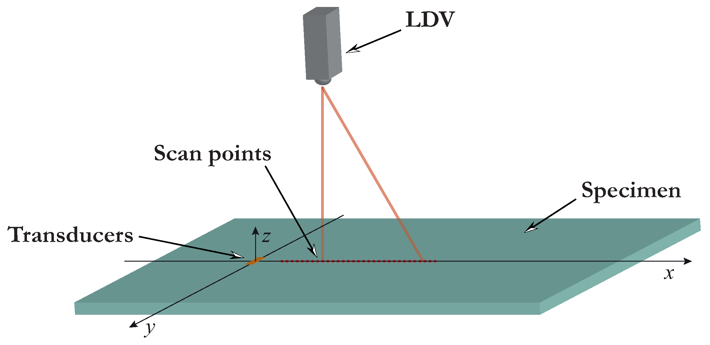
In the experimental investigations, a rectangular aluminium plate (5754 alloy) with dimensions $600\times 600\times 2$ mm${}^3$ is employed, see Figure 2. Ultrasonic GWs are excited by a circular piezoelectric actuator of 8 mm radius and $0.2$ mm thickness manufactured from PZT PIC 151 (PI Ceramic GmbH, Lederhose, Germany). It is adhesively attached on one of the plate surfaces at its central point and is driven by broadband 0.5 $\mathsf{\mu }$s rectangular pulse tone burst voltage of 100 V-pp amplitude. Out-of-plane velocities of propagating wave packages are measured at the surface of the specimen by PSV-500-V laser Doppler vibrometer (LDV) (Polytec GmbH, Waldbronn, Germany), which sensing head is placed about 1100 mm above the sample, minimizing the oblique angle laser beam measurement errors [26]. Since the specimen surfaces remained intact with no special treatment for their reflectivity improvement applied, at least 200 times averaging are performed for each measurement point to improve the signal-to-noise ratio. Moreover, high-frequency noise is filtered out from the acquired wavesignals by 3 MHz low-pass filter applied through the vibrometer software.

For the sake of convenience, let us introduce the Cartesian coordinates so that the scan line goes along the $Ox$-axis, and the transducer is situated at the origin of coordinates. The LDV allows measuring out-of-plane velocities $v(x,0,0,t)$ at the surface $z=0$ of the specimen.

The out-of-plane velocities $v(x_i,t_k)=v_{ik}$ measured at points ($x_i,0,0$) at moments of time $t_k$ in the form of B-scans are further post-processed using the MPM to extract corresponding slowness dispersion curves of propagating GWs. According to the MPM, the Fourier transform is applied to $v(x_i,t_k)$ with respect to time-variable for a certain set of frequencies $f_j$, which gives $V(x_i,f_j)=V_i^j$. In the MPM, the singular value decomposition is applied to the matrix composed of $V_i^j$ in order to compute the discrete relation between the wavenumber k and the frequency f following Schöpfer et al. [18]. The MPM returns the complex-valued wavenumbers $k_{ij}$ describing propagating GWs at the frequency $f_j$. Therefore, a set of experimental slownesses $s_{ij}=k_{ij}/f_j$ is obtained after the application of the processing procedure, removing $k_{ij}$, which most likely does not correspond to a propagating GW. Thus, it does not include $k_{ij}$ with large imaginary parts ($|\mathrm{Im}{k}_{ij}H|>0.005$), and $k_{ij}$ corresponding to those points in the slowness-frequency plane ($s,f$), which has the lowest number of neighbouring points.

Therefore, some GWs are not included in the final set and vice versa, some $s_{ij}$ do not match the actual guided wave. The LDV used in this study has an operating frequency range up to 20 MHz. However, since no special treatment to the specimen surface (i.e., spraying of the reflective paint or gluing of the retroreflective film) was applied, the spectrum of the measured signals at the frequencies higher than 2.5–3 MHz was found to be noisy. Thus, to provide better signal-to-noise ratio in the experimental signals, a 3 MHz lowpass filter was applied through the vibrometer software. Since its transition band was within 2.5 and 3 MHz, in the paper we considered frequencies up to 2.5 MHz.

4. Objective Functions for Material Properties Characterization

As soon as slownesses ${\breve{s}}_k$ at frequencies $f_n$ ($n=\overline{1,N_f}$) are extracted from the experimental data, an inverse problem for material properties’ identification is to be formulated and solved. With a certain model parameter vector $\mathit{\theta }$ including Young’s modulus, Poisson’s ratio, and plate thickness, the mathematical model presented in Section 2 can be applied for computing slownesses as roots of dispersion Equation (7) (for instance, using the method of interval bisection) or the Fourier transform of Green’s matrix (9). Numerical routines for calculating slownesses s and the Fourier transform of Green’s matrix (9) at a given frequency f have been implemented in the FORTRAN programming language. Therefore, an inverse problem is settled, matching the experimental and theoretical results via a specially composed objective function. Two main approaches for the objective function composition are considered here, and the effectiveness of several kinds of objective functions for material properties identification are compared in the subsequent sections.

For both approaches and all the objective functions, the following optimization problem is formulated

$$\widehat{\mathit{\theta }}=arg\underset{\mathit{\theta }\in \mathsf{\Theta }}{min}g(\mathit{\theta },\breve{\mathit{\theta }}).$$

Here $\mathsf{\Theta }$ denotes the bounds of the model parameters of a certain objective function $g(\mathit{\theta },\breve{\mathit{\theta }})$, where the unknown parameter $\breve{\mathit{\theta }}$ incorporates information on the actual value of the parameter, and $\widehat{\mathit{\theta }}$ is an estimate determined as a result of solving the optimization problem. The solution of the optimization problem has been implemented in the Python programming language using the Broyden–Fletcher–Goldfarb–Shanno (BFGS) method [27].

4.1. Objective Function Using Residual of Slownesses

In the first approach, the multi-parameter criterion is the minimization of the residual between measured slownesses ${\breve{s}}_k$ and slownesses $s_k$ calculated by employing the mathematical model described in Section 2 with the parameter $\mathit{\theta }$. Therefore, an iterative correction of simulation results is to be performed with varying material properties $\mathit{\theta }$ until the optimal match between slowness-frequency pairs is found ($s_k(\mathit{\theta },f_n),f_n$), calculated using a theoretical model with parameters $\mathit{\theta }$ and the experiment (${\breve{s}}_k(\breve{\mathit{\theta }},f_n),f_n$), which contain information about the unknown parameter vector $\breve{\mathit{\theta }}$, as well as other factors affecting the experiment. Experimentally determined slownesses are denoted as ${\breve{s}}_k(\breve{\mathit{\theta }},f_n)$ to show straightforwardly that information about actual material properties $\breve{\mathit{\theta }}$ is included into the data.

Formally, the optimal model parameters $\widehat{\mathit{\theta }}$ are obtained from the minimization of the objective function

$$F(\mathit{\theta },\breve{\mathit{\theta }})=\frac{1}{N}\sum _{n=1}^{N_f}\sum _{k\in {\mathcal{P}}_n}|{\breve{s}}_k(\breve{\mathit{\theta }},f_n)-s_k(\mathit{\theta },f_n)|$$

(10)

is composed assuming the modal decomposition of the data. Here, k is the index of experimentally found out data for some frequency $f_n,$ i.e., ${\mathcal{P}}_n=\left\{k\right|\exists {\breve{s}}_k(\breve{\mathit{\theta }},f_n),n=\overline{1,N_f}\}$, $N_f$ is the number of all frequencies, and N is the total number of pairs. Weights can also be used to take into account the sensitivity of the modes to the material properties changes, while such an investigation is out of the scope of the present study and the weights are assumed to be equal. The disadvantage of the employment of this objective function is the necessity of the numerical search of the roots of the dispersion Equation (7) for all dissimilar frequencies ${\breve{s}}_k(\breve{\mathit{\theta }},f_n)$ and the determination of slownesses $s_k(\mathit{\theta },f_n)$ corresponding to the experimental ones.

4.2. Objective Function Based on the Fourier Transform of Green’s Matrix

The second approach avoids time-consuming root search procedure. Moreover, instead of direct insertion of the experimentally determined slowness-frequency pairs (${\breve{s}}_k(\breve{\mathit{\theta }},f_n),f_n$) into dispersion Equation (7), they are substituted into the inversion of the Fourier transform of Green’s matrix $K_{22}^{-1}(f,s,0,\mathit{\theta })$ as proposed in [14]. 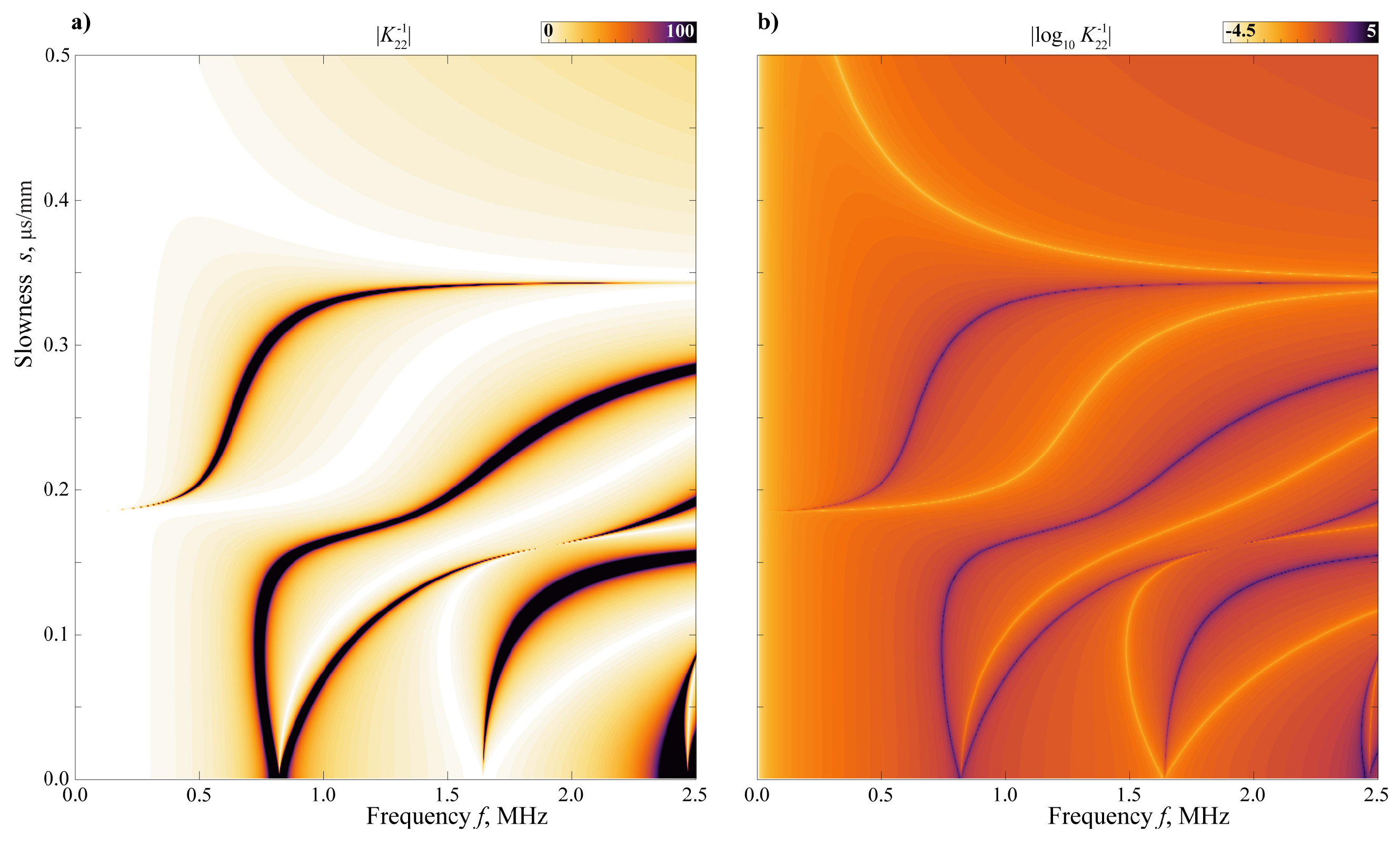The latter provides a smoother surface compared with $\Delta (f,s)$, an example of dispersion map $|K_{22}^{-1}(f,s,0,\mathit{\theta })|$ is demonstrated in Figure 3a for typical aluminium parameters $\mathit{\theta }=\{70\mathrm{GPa},0.33,1.9\mathrm{mm}\}$ (here all values $|K_{22}^{-1}(f,s,0,\mathit{\theta })|>100$ are substituted by 100). In this case, the following objective function is employed:

$$G_{\beta }(\mathit{\theta },\breve{\mathit{\theta }})=\frac{1}{N}\sum _{n=1}^{N_f}\sum _{k\in {\mathcal{P}}_n}min\left(|K_{22}^{-1}(f_n,{\breve{s}}_k(\breve{\mathit{\theta }},f_n),0,\mathit{\theta })|,\beta \right).$$

(11)

Here, an additional parameter $\beta$ is introduced in order to avoid large values of objective function (11), which improves the effectiveness of the inversion procedure, since extremely large values (visible in Figure 3b) could strongly influence the objective function, if, for instance, some points related to noise are included. Another alternative for avoiding too large values of the objective function is the employment of a logarithm procedure so that objective functions

$$H_{\beta }(\mathit{\theta },\breve{\mathit{\theta }})=\frac{1}{N}\sum _{n=1}^{N_f}\sum _{k\in {\mathcal{P}}_n}lnmin\left(|K_{22}^{-1}(f_n,{\breve{s}}_k(\breve{\mathit{\theta }},f_n),0,\mathit{\theta })|,\beta \right)$$

and

$$J_{\beta }(\mathit{\theta },\breve{\mathit{\theta }})=\frac{1}{N}\sum _{n=1}^{N_f}\sum _{k\in {\mathcal{P}}_n}{log}_{10}min\left(\left|K_{22}^{-1}(f_n,{\breve{s}}_k(\breve{\mathit{\theta }},f_n),0,\mathit{\theta })\right|,\beta \right),$$

which are also considered in this study. An example of dispersion map ${log}_{10}\left|K_{22}^{-1}(f,s,0,\mathit{\theta })\right|$ is shown in Figure 3b for the same parameters $\mathit{\theta }$ as used for Figure 3a.

5. Generation of Test Data Sets

In the case of the data obtained from a physical experiment, slownesses can be represented as a sum of the slownesses depending on the material parameters and the random component $ϵ$ included the actions of random factors during the experiment, which can be represented as follows for a given discrete data set

$${\breve{s}}_k(\breve{\mathit{\theta }},f_n)=s_k(\breve{\mathit{\theta }},f_n)+{\epsilon }_{nk}.$$

To obtain statistics proving the effectiveness of the identification procedure, the method must be validated in numerous tests, where the material properties $\breve{\mathit{\theta }}\in \mathsf{\Theta }$ are known, but the data have to simulate the experimental data. For this purpose, test data sets, i.e., slowness–frequency pairs, are to be prepared at first.

At the first stage of the test data preparation, theoretical slownesses are calculated for a known parameter $\breve{\mathit{\theta }}={\mathit{\theta }}^{*}$ at the set of frequencies ${\left\{f_n^{\prime }\right\}}_{n=1}^{N^{\prime }}.$ Since the number of propagating guided waves varies with frequency, slowness–frequency pairs are split into sets $s_k({\mathit{\theta }}^{*},f_n^{\prime })$ of various numbers of elements $M_k^{\prime }$ in the general case, and each set corresponds to a kth non-attenuating guided wave. Next, white noise $\breve{ϵ}\sim N(0,\sigma )$ with the standard deviation $\sigma$ is added so that

$$s_k^{\prime }({\mathit{\theta }}^{*},f_n^{\prime })=s_k({\mathit{\theta }}^{*},f_n^{\prime })(1+\breve{ϵ})$$

is generated independently, and corrupted data sets ($s_k^{\prime }({\mathit{\theta }}^{*},f_n^{\prime }),f_n^{\prime }\}$) are prepared for each guided wave.

At the next stage, the noisy slownesses $s_k^{\prime }({\mathit{\theta }}^{*},f_n^{\prime })$ are damaged for getting a given percentage $\delta$ of gaps in the dispersion curves. To this end, the parameter ${\delta }_1\in (0,1]$ describing the percentage of sole points to be removed from initial data and the parameter ${\delta }_2\in (0,1]$ describing percentage of points belonging to the chains of random lengths to be deleted from $s_k^{\prime }({\mathit{\theta }}^{*},f_n^{\prime })$ are introduced so that $\delta ={\delta }_1+{\delta }_2<1$.

For simplicity, let us introduce one-dimensional arrays of frequencies related to the kth guided wave as follows:

$$\left\{f_{nk}^{\prime }\right\}=\left\{f_n^{\prime }\right|\mathrm{Im}{s}_k^{\prime }({\mathit{\theta }}^{*},f_n^{\prime })=0\}.$$

and denote their lengths as $M_k^{\prime }=\left|{\left\{f_{nk}^{\prime }\right\}}_n\right|$. Next, the number of slowness–frequency pairs for each guided wave, which are expected at the final stage, are defined by the relation $M_k=M_k^{\prime }-M_k^1-M_k^2$, where $M_k^1=\left]M_k^{\prime }{\delta }_1\right[$ is the number of individual points to be excluded from the initial set at random positions, while $M_k^2=\left]M_k^{\prime }{\delta }_2\right[$ is the number of points in $L_k=\mathrm{random}(2,7)$ chains to also be deleted at random positions. To obtain

$${\breve{s}}_k({\mathit{\theta }}^{*},f_n)=\bigcup \left\{s_k^{\prime }({\mathit{\theta }}^{*},f_{n^{\prime }k}^{\prime })|n^{\prime }\notin {\mathcal{I}}_k,n^{\prime }\in \overline{1,M_k^{\prime }}\right\},$$

the auxiliary set

$${\mathcal{I}}_k=\left(\bigcup _{j=1}^{M_k^1}\left\{{\mathcal{A}}_{kj}\right\}\right)\cup \left(\bigcup _{j=1}^{L_k}\left\{{\mathcal{B}}_{kj}\right\}\right)$$

is composed of indices of slowness–frequency pairs to be deleted from the initially generated set $s_k({\mathit{\theta }}^{*},f_n^{\prime })$ employing temporary sets

$${\mathcal{A}}_{kj}=\mathrm{random}(1,M_k^{\prime })$$

and

$${\mathcal{B}}_{kj}=\left\{b_{kj},\dots ,b_{kj}+l_{kj}\right\},$$

where

$$b_{kj}=\mathrm{random}(1,M_k^{\prime }),$$

$$l_{kj}=\mathrm{random}(2,M_k^2),$$

$$\sum _{j=1}^{L_k}\left|l_{kj}\right|=M_k^2,b_{kj}+l_{kj}\le M_k^{\prime },$$

$${\mathcal{A}}_{kj}\bigcap {\mathcal{A}}_{k{j}^{\prime }}={\mathcal{B}}_{kj}\bigcap {\mathcal{B}}_{k{j}^{\prime }}={\mathcal{A}}_{kj}\bigcap {\mathcal{B}}_{k{j}^{\prime }}=\varnothing ,\forall j\ne j^{\prime }.$$

The latter allows us to simulate data gaps and white noise, which are usually observed in experimental data [20,28].

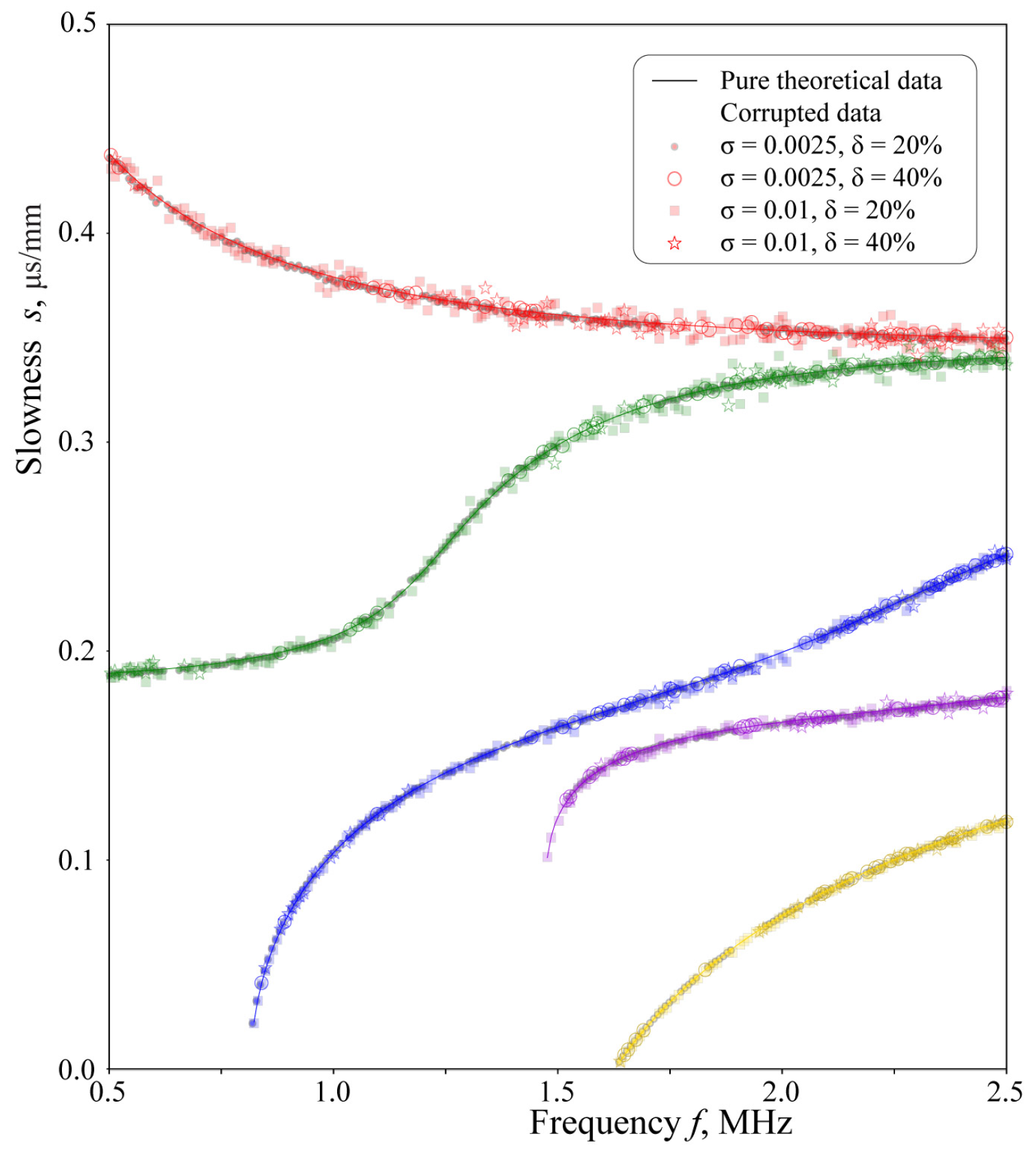
The sets (${\breve{s}}_k({\mathit{\theta }}^{*},f_n),f_n$) generated according to the procedure described above are employed further to analyse the behaviour of the proposed objective functions. Figure 4 shows four corrupted data sets (${\breve{s}}_k({\mathit{\theta }}^{*},f_n),f_n$) for two values of the standard deviation ($\sigma =0.0025$ and $\sigma =0.01$) and two levels of corruption ($\delta =20\%$ and $\delta =40\%$) for ${\mathit{\theta }}^{*}=\{70\mathrm{GPa},0.33,1.9\mathrm{mm}\}$.

6. Numerical Analysis

6.1. Analysis of the Properties of Objective Functions

Some guided waves in laminates may have very low vertical amplitudes or might be poorly excited by the transducer. To emulate the variety of the possible measurement results, including the worst-case scenarios mentioned above, the numerical studies for values of $delta$ varying from 0% to 80% (if the delta is about 80%, the experimental data might be totally useless) have been performed. The conclusions are valid for all the considered values of $delta$, so $delta$, which are typical for the experiments and usually lie in the range between 20% and 40%, and have been chosen for the numerics. For all the data samples depicted in Figure 4, the two-dimensional surfaces $f(E,0.33,H)$, $f(E,\nu ,1.9\mathrm{mm})$ and $f(70\mathrm{GPa},\nu ,H)$ are depicted in Figure 5, Figure 6 and Figure 7 as contour plots of three slices ($\nu =0.33$, $H=1.9\mathrm{mm}$ and $E=70\mathrm{GPa}$) calculated for two objective functions (F and $G_1$ are calculated for the corrupted data ${\breve{s}}_k({\mathit{\theta }}^{*},f_n)$ at $\sigma =0.0075$ and $\delta =20\%$). These figures demonstrate that both objective functions are smooth, and the global minimum, which is clearly visible for both objective functions in Figure 5, Figure 6 and Figure 7, could be determined at the next stage, where the minimization problem is solved. One can also note that objective function F is usually smoother than $G_1$.

6.2. Inverse Problem Solution Using Synthesized Data

Foremost, the material properties identification procedure has been validated using synthesized data ${\breve{s}}_k({\mathit{\theta }}^{*},f_n)$ calculated for ${\mathit{\theta }}^{*}=\{70\mathrm{GPa},0.33,1.9\mathrm{mm}\}$ with different levels of noise $\sigma$ and corruption $\delta =40$%. The statistics have been estimated for Young’s modulus E, Poisson’s ratio $\nu$, and plate thickness H using five different objective functions $F,G_1,G_{100},H_1,J_{150}$ and employing 1000 tests for synthesized data. Figure 8, Figure 9 and Figure 10 depict the lengths of confidence intervals in subplots (a, c, e, g), whereas the relative error

$$\widehat{\mathit{ϵ}}=\frac{\mathrm{E}\left(\widehat{\mathit{\theta }}\right)-{\mathit{\theta }}^{*}}{{\mathit{\theta }}^{*}}.$$

is illustrated in the subplots (b, d, f, h). Here, the mean of the parameter estimates $\widehat{\mathit{\theta }}$ is employed as an estimate for the expectation $\mathrm{E}\left(\widehat{\mathit{\theta }}\right)$. The length of the confidence interval for the mean indirectly indicates the efficiency of the estimates, which characterizes the accuracy of the obtained parameter estimates and allows us to compare the objective functions from this point of view. The relative error vector $\widehat{\mathit{ϵ}}$ can be used to consider a property such as biased or unbiased parameter estimates. To investigate the influence of the presence of guided waves, various combinations of guided waves has been considered (markers in the bottom of Figure 8, Figure 9 and Figure 10 show which modes have been included in the data set).

According to Figure 8, Figure 9 and Figure 10, one can conclude that the estimates of all parameters determined using the objective function F, which summarizes residuals in slownesses, are unbiased and show the most efficiency for all the considered combinations of guided waves except for GW 1. However, it should be noted that all estimates for the only first guided wave GW 1, which is the fundamental antisymmetric mode, are biased. The objective function $G_{\beta }$ gives the more efficiency and less biased estimates for $\beta =1$ than $\beta =100$ for the majority of the considered synthesized data sets. Compared to the objective functions $H_1$ and $J_{150}$, the functional $G_1$ also provides more accurate estimates.

In general, it should be mentioned that the majority of the estimates calculated using the approach based on the Fourier transform of Green’s matrix give an underestimated value of Young’s modulus up to 9% (see Figure 8) and an overestimated value of the Poisson’s ratio (more than 10%), see Figure 9. The plate thickness estimates are also more inclined to be underestimated, but the error varies in the 3% range (Figure 10). It is also noteworthy that the most efficient and less biased estimates for Young’s modulus and Poisson’s ratio are determined for GW 2 and GW 2–GW 3. This regularity can not be reported for the sample’s thickness, however, the estimation error is small for all the considered combinations of GW modes. It should also be noted that the computational time for the approach based on the slowness residuals is hundred times smaller than for the approach based on the Fourier transform of Green’s matrix.

6.3. Inverse Problem Solution Using LDV Experimental Data

At the final stage, the two proposed approaches have been tested and validated using experimental data obtained using the LDV setup for a plate made of aluminium alloy 5754 with the mass density $\rho$ = 2660 kg/m${}^3$, with material parameters in dynamic tests that are approximately the following: $\nu =0.35$, $H=2.0\mathrm{mm}$ and $E=71\mathrm{GPa}$ [29]. Figure 11 depicts slownesses (${\breve{s}}_k(\breve{\mathit{\theta }},f_n),f_n$) obtained applying the MPM to the experimental data as circles. The optimization procedure has been run 1000 times using the BFGS method with various starting points uniformly distributed in $10\times 10\times 10$ grid in the parameter $\mathit{\theta }$ space using both objective functions. The statistics obtained for the estimates $\widehat{\mathit{\theta }}$ calculated using objective function F based on the slowness residuals are given in

Table 1. The cumulative percentages and the mean for the results calculated using objective function F based on the slowness residuals.

GW Modes	Statistics
	2.5%	97.5%	50%	mean
	Young’s modulus
	69.44067	70.02778	69.53528	69.57336
	70.85072	70.93444	70.89058	70.86935
	70.57222	70.99317	70.94851	70.86905
	Poisson’s ratio
	0.2814911	0.3088387	0.2851565	0.2868929
	0.3426350	0.345837	0.3443798	0.345837
	0.3498317	0.352299	0.3513940	0.3512925
	Thickness
	2.038286	2.045689	2.044301	2.043785
	2.019506	2.022150	2.020586	2.020512
	2.001522	2.014291	2.013035	2.010527

, while the statistic estimations related to the objective function $G_1$ based on the Fourier transform of Green’s matrix are presented in

Table 2. The cumulative percentages and the mean for the results calculated using objective function $G_1$ based on Green’s matrix.

GW Modes	Statistics
	2.5%	97.5%	50%	mean
	Young’s modulus
	70.51223	70.55632	70.53855	70.54622
	68.29054	70.90552	70.88853	70.71145
	68.94975	71.68033	71.39863	71.13951
	Poisson’s ratio
	0.3130311	0.3199611	0.3156035	0.3164631
	0.2584863	0.3394943	0.3394111	0.3352184
	0.2730250	0.3862568	0.3508503	0.3454789
	Thickness
	2.050283	2.058020	2.056627	2.055417
	1.985751	2.081555	2.029845	2.029940
	2.008208	2.090551	2.030139	2.034077

. In these tables, the boundaries of the intervals, where 95% of all calculated parameters are located, as well as the medians and means, are given. The results presented in these tables have been computed for the following sets of modes: GW 1–GW 2, GW 2–GW 3, and GW 1–GW 5. The conclusions that can be drawn from the analysis of Table 1 and Table 2 are consistent with the results obtained for the synthesized data provided in Section 6.2. The parameter estimates found for the approach using slowness residuals are more accurate, since the lengths of confidence intervals are narrower. At the same time, the obtained values are slightly underestimated for Young’s modulus and Poisson’s ratio and slightly overestimated for the thickness for the mode set GW 1–GW 2. It has been observed by [30] that the dispersion curves of A0 mode for a broad frequency range demonstrate rather low sensitivity even to the essential changes in Young’s modulus and Poisson’s ratio. Therefore, if being employed in the reconstruction procedure (as in the considered case of GW 1–GW 2), it could provide higher dispersion and discrepancies in the obtained results. As the final estimate of the faithful parameters, both the median and the mean values can be taken, since their values are very close. For calculations by means of the approach based on Green’s matrix, only the results obtained for the set of modes GW 1–GW 5 can be considered acceptable.

Figure 11 depicts the slownesses calculated as a solution of dispersion Equation (7) for parameters estimated using the developed numerical routines (solid, dashed, dash-dotted lines), the corresponding values of $\widehat{\mathit{\theta }}$ are given in Table 1 and Table 2 (see the last column for the mean value). Four sets of slowness curves corresponding to $\widehat{\mathit{\theta }}$ determined using experimental data (${\breve{s}}_k(\breve{\mathit{\theta }},f_n),f_n$) and two approaches employing data for modes GW 1–GW 2 (dashed and thick solid lines) and GW 1–GW 5 (dash-dotted and thin solid lines) are demonstrated in Figure 11. A sufficient discrepancy between theoretical curves and the experimental data is clearly visible by eye for modes GW 1–GW 2. For the full data set, including information on all modes GW 1–GW 5, both approaches have more or less similar difference with experimentally obtained slownesses, though the approach based on the slowness residuals provide material properties slightly more close to the actual ones. This conclusion is made based on the knowledge that the actual measured thickness value $H=2$ mm, and the result of numerical experiments presented in Section 6.2.

7. Discussions

The proposed automated procedure is an attempt to summarize and extend the results of the researchers mentioned in the introduction as well as many others, who used GWs for material properties characterization. The comparison of two different approaches for objective function composition for the proposed procedure has shown that both approaches have some advantages as well as disadvantages. The approach using the Fourier transform of Green’s matrix is much faster compared with the approach using discrepancy between theoretical and experimental slownesses. The authors believe that the advantages of the two approaches might be combined into an improved algorithm with low computational costs and accuracy close to the approach using slownesses. In this study, a sufficient influence of the number of propagating modes on the accuracy of the identification was shown, which might be useful for improved algorithms based on both the approaches considered in this paper.

Though the proposed procedure for material properties identification has been validated and verified for an elastic isotropic waveguide, it can be naturally extended for multi-layered structures and damaged laminates, e.g., considering the data from the previous authors’ studies [20,28]. Another possible extension of the algorithm is the properties characterization of piezoelectric and anisotropic layered structures using information about the properties of guided waves propagating there. Besides, it is not limited by the matrix pencil method and laser Doppler vibrometry. The most important basis of the developed procedure is careful extraction of the information about dispersion characteristics of the layered waveguide and fast computational algorithms for Green’s matrices, which have been recently advanced by the authors [31,32] and can be employed in the near future.

References

1. Pagnotta, L. Determining elastic constants of materials with interferometric techniques. Inverse Probl. Sci. Eng. 2006, 14, 801–818. [Google Scholar] [CrossRef]
2. Kam, T.; Chen, C.; Yang, S. Material characterization of laminated composite materials using a three-point-bending technique. Compos. Struct. 2009, 88, 624–628. [Google Scholar] [CrossRef]
3. Tam, J.; Ong, Z.; Ismail, Z.; Ang, B.; Khoo, S. Identification of material properties of composite materials using nondestructive vibrational evaluation approaches: A review. Mech. Adv. Mater. Struct. 2017, 24, 971–986. [Google Scholar] [CrossRef]
4. Tam, J.H. Identification of elastic properties utilizing non-destructive vibrational evaluation methods with emphasis on definition of objective functions: A review. Struct. Multidiscip. Optim. 2020, 61, 1677–1710. [Google Scholar] [CrossRef]
5. Chen, Q.; Xu, K.; Ta, D. High-resolution Lamb waves dispersion curves estimation and elastic property inversion. Ultrasonics 2021, 115, 106427. [Google Scholar] [CrossRef]
6. Okumura, S.; Nguyen, V.H.; Taki, H.; Haïat, G.; Naili, S.; Sato, T. Phase velocity estimation technique based on adaptive beamforming for ultrasonic guided waves propagating along cortical long bones. Jpn. J. Appl. Phys. 2017, 56, 07JF06. [Google Scholar] [CrossRef] [Green Version]
7. Okumura, S.; Nguyen, V.H.; Taki, H.; Haïat, G.; Naili, S.; Sato, T. Rapid High-Resolution Wavenumber Extraction from Ultrasonic Guided Waves Using Adaptive Array Signal Processing. Appl. Sci. 2018, 8, 652. [Google Scholar] [CrossRef] [Green Version]
8. Bochud, N.; Laurent, J.; Bruno, F.; Royer, D.; Prada, C. Towards real-time assessment of anisotropic plate properties using elastic guided waves. J. Acoust. Soc. Am. 2018, 143, 1138–1147. [Google Scholar] [CrossRef] [Green Version]
9. Webersen, M.; Johannesmann, S.; Düchting, J.; Claes, L.; Henning, B. Guided ultrasonic waves for determining effective orthotropic material parameters of continuous-fiber reinforced thermoplastic plates. Ultrasonics 2018, 84, 53–62. [Google Scholar] [CrossRef]
10. Tian, Z.; Yu, L. Lamb wave frequency-wavenumber analysis and decomposition. J. Intell. Mater. Syst. Struct. 2014, 25, 1107–1123. [Google Scholar] [CrossRef]
11. Eremin, A.; Glushkov, E.; Glushkova, N.; Lammering, R. Evaluation of effective elastic properties of layered composite fiber-reinforced plastic plates by piezoelectrically induced guided waves and laser Doppler vibrometry. Compos. Struct. 2015, 125, 449–458. [Google Scholar] [CrossRef]
12. Eremin, A.A.; Golub, M.V.; Wilde, M.V.; Pleshkov, V.N. Influence of retroreflective films on the behaviour of elastic guided waves measured with laser Doppler vibrometry. Measurement 2022, 190, 110572. [Google Scholar] [CrossRef]
13. Takahashi, V.; Lematre, M.; Fortineau, J.; Lethiecq, M. Elastic parameters characterization of multilayered structures by air-coupled ultrasonic transmission and genetic algorithm. Ultrasonics 2022, 119, 106619. [Google Scholar] [CrossRef]
14. Lu, L.; Charron, E.; Glushkov, E.; Glushkova, N.; Bonello, B.; Julien, F.H.; Gogneau, N.; Tchernycheva, M.; Boyko, O. Probing elastic properties of nanowire-based structures. Appl. Phys. Lett. 2018, 113, 161903. [Google Scholar] [CrossRef] [Green Version]
15. Pagnotta, L.; Stigliano, G. Elastic characterization of isotropic plates of any shape via dynamic tests: Practical aspects and experimental applications. Mech. Res. Commun. 2009, 36, 154–161. [Google Scholar] [CrossRef]
16. Wilde, M.V.; Golub, M.V.; Eremin, A.A. Experimental observation of theoretically predicted spectrum of edge waves in a thick elastic plate with facets. Ultrasonics 2019, 98, 88–93. [Google Scholar] [CrossRef]
17. Tu, J.H.; Rowley, C.W.; Luchtenburg, D.M.; Brunton, S.L.; Kutz, J.N. On dynamic mode decomposition: Theory and applications. J. Comput. Dyn. 2014, 1, 391–421. [Google Scholar] [CrossRef] [Green Version]
18. Schöpfer, F.; Binder, F.; Wöstehoff, A.; Schuster, T.; von Ende, S.; Föll, S.; Lammering, R. Accurate determination of dispersion curves of guided waves in plates by applying the matrix pencil method to laser vibrometer measurement data. CEAS Aeronaut. J. 2013, 4, 61–68. [Google Scholar] [CrossRef]
19. Chamaani, S.; Akbarpour, A.; Helbig, M.; Sachs, J. Matrix Pencil Method for Vital Sign Detection from Signals Acquired by Microwave Sensors. Sensors 2021, 21, 5735. [Google Scholar] [CrossRef]
20. Wilde, M.V.; Golub, M.V.; Eremin, A.A. Elastodynamic behaviour of laminate structures with soft thin interlayers: Theory and experiment. Materials 2022, 15, 1307. [Google Scholar] [CrossRef]
21. Thelen, M.; Bochud, N.; Brinker, M.; Prada, C.; Huber, P. Laser-excited elastic guided waves reveal the complex mechanics of nanoporous silicon. Nat. Commun. 2021, 12, 3597. [Google Scholar] [CrossRef] [PubMed]
22. Liu, Z.; Xu, K.; Li, D.; Ta, D.; Wang, W. Automatic mode extraction of ultrasonic guided waves using synchrosqueezed wavelet transform. Ultrasonics 2019, 99, 105948. [Google Scholar] [CrossRef] [PubMed]
23. Fairuschin, V.; Brand, F.; Backer, A.; Drese, K.S. Elastic Properties Measurement Using Guided Acoustic Waves. Sensors 2021, 21, 6675. [Google Scholar] [CrossRef] [PubMed]
24. Lan, B. Non-iterative, stable analysis of surface acoustic waves in anisotropic piezoelectric multilayers using spectral collocation method. J. Sound Vib. 2018, 433, 16–28. [Google Scholar] [CrossRef]
25. Grünsteidl, C.; Murray, T.W.; Berer, T.; Veres, I.A. Inverse characterization of plates using zero group velocity Lamb modes. Ultrasonics 2016, 65, 1–4. [Google Scholar] [CrossRef] [Green Version]
26. Neumann, M.N.; Hennings, B.; Lammering, R. Identification and Avoidance of Systematic Measurement Errors in Lamb Wave Observation With One-Dimensional Scanning Laser Vibrometry. Strain 2013, 49, 95–101. [Google Scholar] [CrossRef]
27. Fletcher, R. Practical Methods of Optimization, 2nd ed.; John Wiley & Sons: New York, NY, USA, 2000; p. 436. [Google Scholar]
28. Golub, M.V.; Doroshenko, O.V.; Wilde, M.V.; Eremin, A.A. Experimental validation of the applicability of effective spring boundary conditions for modelling damaged interfaces in laminate structures. Compos. Struct. 2021, 273, 114141. [Google Scholar] [CrossRef]
29. Kammer, C. Aluminium Taschenbuch: Band 1: Grundlagen und Werkstoffe; Beuth Verlag: Berlin, Germany, 2021; p. 790. [Google Scholar]
30. Rogers, W.P. Elastic property measurement using Rayleigh-Lamb waves. Res. Nondestruct. Eval. 1995, 6, 185–208. [Google Scholar] [CrossRef]
31. Fomenko, S.I.; Golub, M.V.; Doroshenko, O.V.; Wang, Y.; Zhang, C. An advanced boundary integral equation method for wave propagation analysis in a layered piezoelectric phononic crystal with a crack or an electrode. J. Comput. Phys. 2021, 447, 110669. [Google Scholar] [CrossRef]
32. Glushkov, E.; Glushkova, N.; Eremin, A.; Lammering, R. Group velocity of cylindrical guided waves in anisotropic laminate composites. J. Acoust. Soc. Am. 2014, 135, 148–154. [Google Scholar] [CrossRef]
Figure 1. Geometry of the problem.
Symmetry 14 01077 g001
Figure 2. Experimental setup.
Symmetry 14 01077 g002
Figure 3. Surfaces of the dispersion maps for | K 22 1 ( f , s , 0 , θ ) | (a) and log 10 | K 22 1 ( f , s , 0 , θ ) | (b) at θ = { 70 GPa , 0.33 , 1.9 mm } .
Symmetry 14 01077 g003
Figure 4. Examples of artificially generated corrupted slowness-frequency pairs ( s ˘ k ( θ * , f n ) , f n ) for θ * = { 70 GPa , 0.33 , 1.9 mm } .
Symmetry 14 01077 g004
Figure 5. Surfaces of objective functions F ( θ ˜ ) (ad) and G 1 ( θ ˜ ) (eh) at θ ˜ = ( E , ν = 0.33 , H ) and for different degrees of corruptness σ ( δ = 0.4 ).
Symmetry 14 01077 g005
Figure 6. Surfaces of objective functions F ( θ ˜ ) (ad) and G 1 ( θ ˜ ) (eh) at θ ˜ = ( 70 GPa , ν , H ) for different degrees of corruptness ( δ = 0.4 ).
Symmetry 14 01077 g006
Figure 7. Surfaces of objective functions F ( θ ˜ ) (ad) and G 1 ( θ ˜ ) (eh) at θ ˜ = ( E , ν , 1.9 mm ) for different degrees of corruptness σ ( δ = 0.4 ).
Symmetry 14 01077 g007
Figure 8. The length of confidence intervals (a,c,e,g) and the relative error ϵ ^ 1 (b,d,f,h) for Young’s modulus E identification obtained using five objective functions F , G 1 , G 100 , H 1 , J 150 for different levels of noise σ at δ = 40 %.
Symmetry 14 01077 g008
Figure 9. The length of confidence intervals (a,c,e,g) and the relative error ϵ ^ 2 (b,d,f,h) for Poisson’s ratio ν identification obtained using five objective functions F , G 1 , G 100 , H 1 , J 150 for different levels of noise σ at δ = 40 %.
Symmetry 14 01077 g009
Figure 10. The length of confidence intervals (a,c,e,g) and the relative error ϵ ^ 3 (b,d,f,h) for plate thickness H identification obtained using five objective functions F , G 1 , G 100 , H 1 , J 150 for different levels of noise σ at δ = 40 %.
Symmetry 14 01077 g010
Figure 11. Experimentally observed (circles) and theoretically predicted slownesses (lines) calculated at θ ^ estimated using objective function F based on the slowness residuals (solid lines) and G 1 based on Green’s matrix (dash-dotted and dashed lines) for GW 1–GW 2 (dashed and thick solid lines) and GW 1–GW 5 (dash-dotted and thin solid lines).
Symmetry 14 01077 g011