Particle Swarm Optimization Embedded in UAV as a Method of Territory-Monitoring Efficiency Improvement

Abstract

Unmanned aerial vehicles have large prospects for organizing territory monitoring. To integrate them into this sphere, it is necessary to improve their high functionality and safety. Computer vision is one of the vital monitoring aspects. In this paper, we developed and validated a methodology for terrain classification. The overall classification procedure consists of the following steps: (1) pre-processing, (2) feature extraction, and (3) classification. For the pre-processing stage, a clustering method based on particle swarm optimization was elaborated, which helps to extract object patterns from the image. Feature extraction is conducted via Gray-Level Co-Occurrence Matrix calculation, and the output of the matrix is turned into the input for a feed-forward neural network classification stage. The developed computer vision system showed 88.7% accuracy on the selected test set. These results can provide high quality territory monitoring; prospectively, we plan to establish a self-positioning system based on computer vision.

1. Introduction

With the development of Industry 4.0, a tendency to automate time and resource-intensive routine processes has been noticed. Production, transportation, cloud computations, and monitoring can be classified as such categories of processes. Industry 4.0 intends to integrate the cyber–physical concept into the different spheres of life, which means that with automation, people can focus on more complicated tasks, such as planning, engineering, and programming.

This paper studies the task of area monitoring. Under monitoring, we consider a regular observation of a given territory with the aim of finding anomalies. To organize monitoring, UAVs can be used.

Monitoring by dint of UAVs has become a more relevant aspect, as UAVs’ abilities exceed human physical possibilities to collect and process information; UAVs can operate in critical situations and can collect quantitative and qualitative data with sensors. Examples of successful applications can include simple domestic tasks [1], border control [2], and coast patrol [3], among several other examples that could be mentioned. In addition, UAVs can work in conditions unsuitable for a human, such as emergencies [4]. Thus, drones are more effective and require fewer resources in the context of territory monitoring.

This paper is an extension of the work [5]. It contains an extended formalization of the developed computer vision algorithm. In addition, a combination of computer vision and map projection is presented, which is a good foundation for the vision-based geolocation system development in the sphere of geographic information systems.

In order to report about any non-standard situation, the UAV requires to have knowledge about its own location. However, the GPS does not guarantee geolocation accuracy due to the fact that it is not always available [6]. Taking into account possible GPS signal interruptions, the authors elaborated the system of computer vision that determines the terrain type based on UAV downwash. Prospectively, it is possible to project the classified terrain onto the map and by this define the UAV’s coordinates. This paper contains information about hardware and software elaborated by the authors for territory-monitoring purposes.

The remaining paper is organized as follows: Section 2 describes the existing implementations of UAVs and computer vision systems in the process of monitoring; Section 3 provides information about the designed UAV system. Section 4 describes the obtained terrain classification results, and Section 5 illustrates the projection of the classification results on the map. Finally, Section 6 concludes the paper by assessing the performed work and planning the next research steps.

2. Related Work

2.1. Monitoring with UAVs

UAVs have been already implemented in some countries or are under discussion in terms of their applicability [7,8,9,10,11,12,13]. For example, the authors of [14] considered the issue of using UAVs in the context of soil-erosion monitoring in Morocco. The UAV flight was to cover landscapes of different scales. The assessment of soil erosion risk was conducted according to Digital Terrain Models that were provided by dint of photogrammetric image processing.

Another implementation of photogrammetry was realized in Portugal [15]. It was embedded in UAVs to monitor the Portuguese northwest coast. The monitoring process was conducted to assess the impact of natural and anthropogenic factors on the state of coastal areas.

Monitoring by UAVs can be effectively used in the context of the detection and prevention of emergencies. For example, in the work [16], the authors described UAV groups as a good option to organize monitoring for emergency response, as emergency zones are usually inaccessible to humans. In addition, UAVs allow one to communicate and react in real-time mode, which is relevant in the context of negative consequences’ prevention.

UAVs have been successfully implemented in the case of natural-disaster monitoring. In the work [17], a system for landslide risk assessment was proposed, consisting of Ground-based Interferometric Synthetic Aperture Radar (GB-InSAR), Terrestrial Laser Scanning (TLS), and a UAV.

UAV systems have been adapted for forest-fire condition monitoring. The authors of the paper [18] elaborated a monitoring system consisting of a UAV equipped with cameras, sensors, and communication modules to provide real-time data collection and data transmission.

2.2. Computer Vision and Pattern Recognition

In the process of monitoring, one of the most important parts of UAVs is the computer vision system, as visual information contains a lot of useful data for detecting and preventing emergency situations. That is why it is essential to provide high accuracy of pattern recognition. The work [19] proposed a system for the fault detection and correction of board cameras.

Visual information processing can be divided into three main stages:

• Image preprocessing—the procedure of removing visible drawbacks of the input image (noise, blur) [20];
• Image preparation for pattern-recognition process—procedure of extracting image features (texture, patterns, contours) [21];
• Pattern recognition—detection and classification of particular objects [22].

2.2.1. Image Preprocessing

This stage is focused on image-quality improvement. Issues such as noise, blur, and uneven contrast are resolved. The aspect of image preprocessing was also discussed in the context of UAV monitoring. In the work [23], a method for image deblurring was described.

Relative to UAVs in agriculture, a pattern-recognition process was described in [24]. In order to prevent diseases and pests in rice sprouts, a system consisting of preprocessing, segmentation, and classification was designed. For the first stage, histogram equalization was used for gray-scale conversion.

The preprocessing stage is relevant in other practical implementations, and its methods can be useful in the field of UAV monitoring, for instance, for illumination issues. In the work [25], a method for the minimization of illumination variance was represented in the field of face recognition. It contributes to brightness equalization and to the increase in pattern-recognition accuracy.

Another preprocessing method proposed for face recognition based on local binary patterns was proposed in the paper [26]. This method was also intended to resolve the issue of illumination variance and to extract the image texture.

The authors consider as a current task of preprocessing during UAV monitoring the following points:

• Denoising;
• Deblurring;
• Brightness equalization.

2.2.2. Image Preparation for Pattern-Recognition Process

During the second stage of visual information processing, one of the ways to increase classification accuracy is image segmentation. This field was thoroughly investigated in the work [27].

Segmentation is the process of dividing a digital image into a set of its constituent regions in order to select objects and their boundaries. There is a variety of elaborated segmentation methods, and each of them can be suitable for particular image categories [28,29,30].

The article [31] provides an overview of segmentation techniques:

• Pixel-based methods;
• Edge-based methods;
• Region-based methods.

One of the segmentation methods is clustering. Image clustering consists of a division of pixels into several non-intersecting groups in such a way that pixels from the same group have similar features; meanwhile, the features of pixels from different groups vary significantly from each other. Until the current moment, plenty of different clustering methods have been elaborated [32].

One of the most widespread clustering methods is k-means [33]. Its main idea consists in minimizing the distance between the objects in the clusters. The algorithm stops running when further minimization becomes impossible.

The other well-known clustering method is fuzzy C-means [34]. The method is based on fuzzy logic, i.e., on the assumption that each object from the given set, to some extent, belongs to a particular cluster from the given set of clusters.

3. System Description

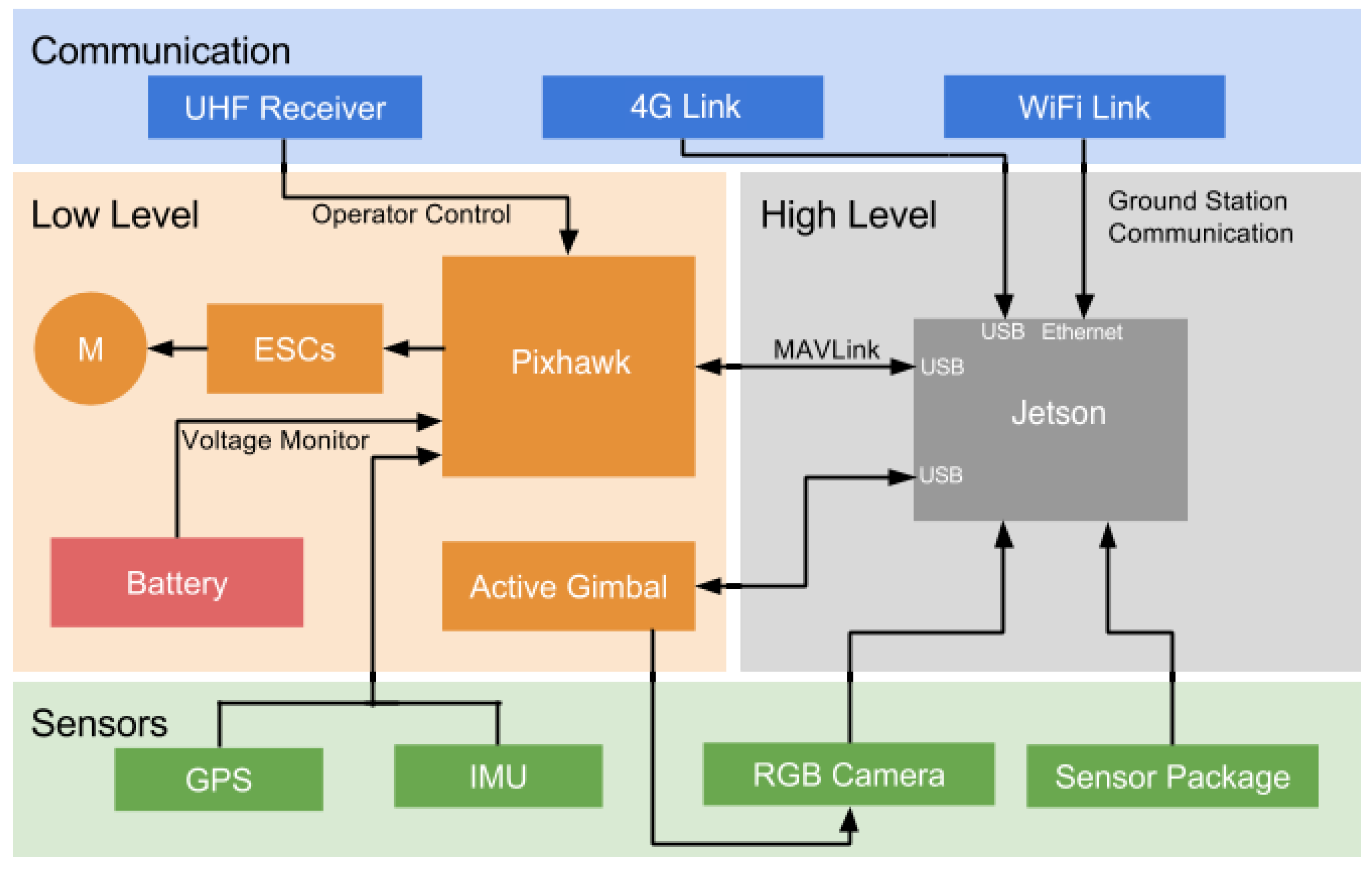
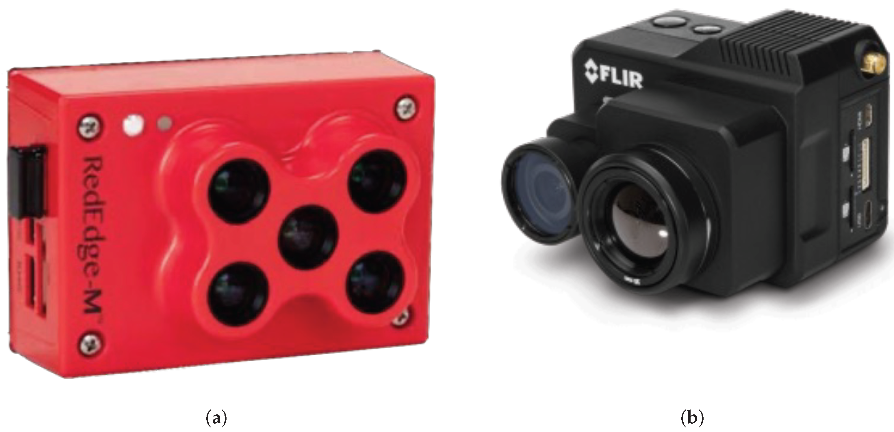
3.1. Hardware

In this section, we explain the hardware used in this paper. One UAV was used in the experiments, known as HEIFU.

The HEIFU is a custom-made solution, aimed at the agricultural sector, developed by a collaboration between BEV and PDMFC. The HEIFU is equipped with an onboard computer running on Ubuntu and a ROS. This is an open platform that allows different inputs to be integrated and is used to run multiple tasks, such as image processing, data relaying, remote control of a drone, and more. The HEIFU can be used with different communication systems, such as a mobile network or Wi-Fi connection. The HEIFU is a hexacopter, as it can be seen in Figure 1, with a dimension of 1.4 m in the diagonal wheelbase. The drone’s weight is around 6.2 kg, including battery, and the hovering time is around 38 min with a battery of 16 Ah.

Some of the HEIFU specifications are:

• Ardupilot (Pixhawk) hardware is used to control low-level operation. This hardware contains an IMU and a GPS to know the UAV’s position and orientation; in addition, the Pixhawk connects to the Jetson nano embedded system via MAVlink protocol and the UAV’s battery; lastly, to control the UAV’s motors, it is connected to a UHF receiver;
• A Jetson nano is used to control high-level operation. It receives data from the distance sensor (depth cameras) and the RGB camera, and it communicates with external devices via Wi-Fi link;
• An RGB camera with a gimbal stabilizer is installed to capture onboard images at a resolution of 640 × 480 pixels;
• The camera and lens specifications are known, allowing the field of view (FOV) and the pixel size in meters to be computed.

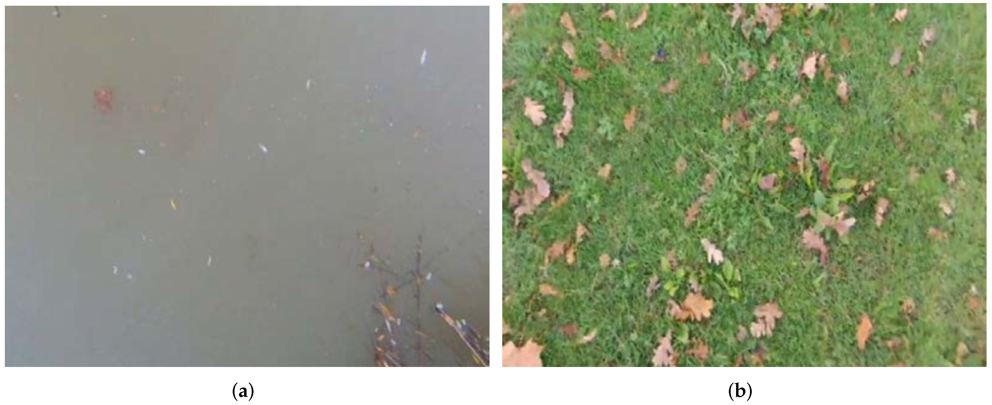
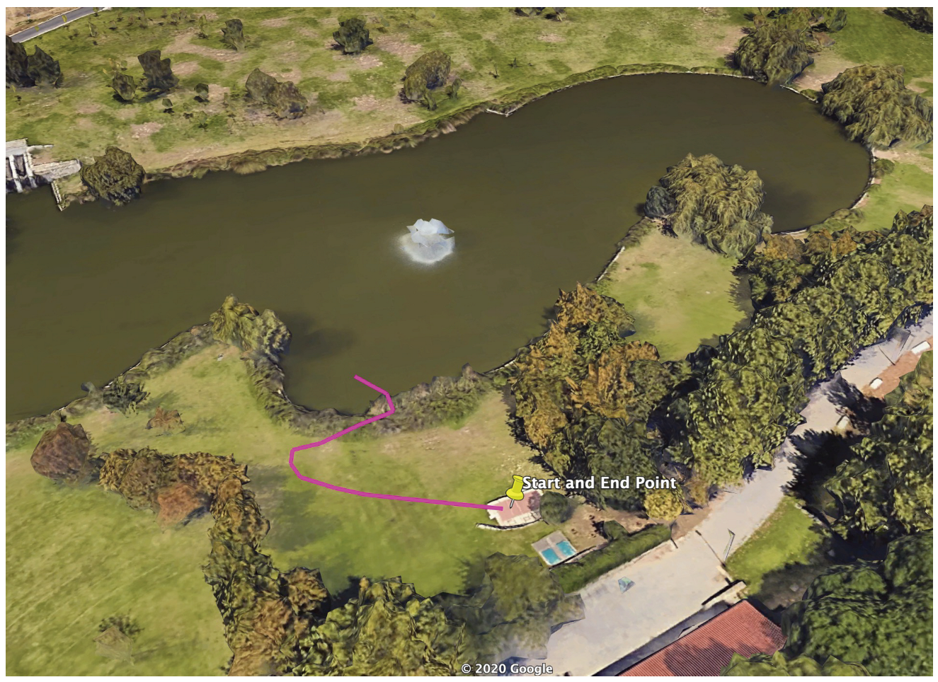
For a better understanding of the communications between various system layers, in Figure 2, the communication layers are represented.

3.2. Data Gathering

Different terrains have singular texture patterns that can be used in their identification. In this paper, for terrain classification, the importance of static features such as color and texture is studied. As can be seen in Figure 3, in this paper, four different terrain types (water, vegetation, asphalt, and sand) are studied.

3.3. Pattern-Recognition Methods

3.3.1. Image Preparation

During monitoring, unexpected situations can occur, and in order not to misclassify them, it is necessary to take into account all the possible predictors. We consider the RGB part of the image as an important component, which is why we decided not to convert the image to gray-scale.

To make the objects on the image insensitive to the light changes and to remove the noise level, normalization was used. It works according to Equation (1):

$$(r^{\prime },g^{\prime },b^{\prime })=\left(\frac{r}{\sqrt{r^2+g^2+b^2}},\frac{g}{\sqrt{r^2+g^2+b^2}},\frac{b}{\sqrt{r^2+g^2+b^2}}\right),$$

(1)

where r, g, and b are the initial values of a pixel’s RGB vector; r’, g’, and b’ are the normalized values of a pixel’s RGB vector.

3.3.2. Particle Swarm Optimization

The existing clustering methods have the following drawbacks:

• Sensitivity to outliers;
• Need to specify clustering parameters beforehand;
• Uncertainty of actions with objects that possess the properties of two different clusters simultaneously.

All the shortcomings were taken into account, and the authors elaborated a clustering method based on a combination of k-means and PSO [35]. The role of PSO consists in automated centroid determination and pixel allocation, i.e., exclusion of human participation from the clustering process.

The general functionality of PSO consists of the following steps:

1.

There is a swarm of particles, and each of them has coordinate $x_i$∈$R^n$ and velocity $v_i$; f is the function that needs to be minimized; $p_i$—the best-known $i_{th}$ particle position; g—the best-known state of the entire swarm;

2.

For each particle $s_i$∈S, it is necessary to:

• Generate an initial position;
• Assign to the best-known position of particle $p_i$ its initial value $x_i$;
• In the case where $f\left(p_i\right)<f\left(g\right)$, there is a necessity to update the value from g to p;
• Generate a particle velocity.

3.

Until the stopping criterion is reached, the following points should be fulfilled for each particle:

• Generate random vectors ${\mathit{r}}_{\mathit{p}}$ and ${\mathit{r}}_{\mathit{s}}$, which have a range of values between 0 and 1;
• Update the particle velocity as in Equation (2):

  $$v_i=w\ast v_i+{\varphi }_p\ast r_p\times (p_i-x_i)+{\varphi }_g\ast r_g\times (g-x_i),$$

  (2)

  where × is a vector product operation, and w, ${\varphi }_p$, and ${\varphi }_g$ are the parameters specified by the user;
• The particle position should be changed according to Equation (3):

  $$x_i=x_i+v_i$$

  (3)
• Compare the values of $f\left(x_i\right)$ and $f\left(p_i\right)$; if the first value is less than the second one, the best-known position of particle $p_i$ should be replaced by $x_i$; if $f\left(p_i\right)<f\left(g\right)$, the value of parameter g is to be changed to the value of $p_i$.

4.

In the end, parameter g contains the best solution.

The algorithm of the elaborated clustering method [36] is as follows:

1.

Image unification: The rounding of $W^{\prime }$ pixels horizontally and $H^{\prime }$ pixels vertically to the nearest values of W and H, respectively, which are multiples of 10, in the normalized image;

2.

Initial cluster distribution: The sequential selection of 10-by-10 regions in the image;

3.

Automated initial centroid allocation: The choosing of the pixel with maximum average intensity; average intensity is calculated as in Equation (4):

$$I_{av}=\frac{r^{\prime }+g^{\prime }+b^{\prime }}{3},$$

(4)

where $r^{\prime }$, $g^{\prime }$, and $b^{\prime }$ are the normalized values of a pixel’s RGB vector;

4.

Cluster merging: The comparison of the rounded average intensity values for centroids from neighboring regions; the comparison is conducted vertically and horizontally relatively to each cluster. If the rounded average intensity values are equal to each other, two neighboring clusters are combined into one. In the merged cluster, the centroid is the pixel with the maximum average intensity value; this step needs to be repeated until there are M clusters $c_j$, j∈$[1,M]$ with the pairwise distinct rounded average intensity values of the centroids. In terms of PSO, the stopping criteria is a situation whereby further cluster merging is impossible, and all the rounded average intensity values are different;

5.

For each pixel, the distance function d and color function f need to be calculated; they are shown in Equation (5) and Equation (6), respectively:

$$d(x_i,c_j)=\sqrt{{(x_{i_w}-c_{j_w})}^2+{(x_{i_h}-c_{j_h})}^2},$$

(5)

where $x_{i_w}$ and $x_{i_h}$ are the coordinates of the given pixel per width and height of the image, and $c_{j_w}$ and $c_{j_h}$ are the coordinates of the centroid per image width and height;

$$f(x_i,c_j)=\sqrt{{(r_{x_i}^{\prime }-r_{c_j}^{\prime })}^2+{(g_{x_i}^{\prime }-g_{c_j}^{\prime })}^2+{(b_{x_i}^{\prime }-b_{c_j}^{\prime })}^2},$$

(6)

where $r_{x_i}^{\prime }$, $g_{x_i}^{\prime }$, and $b_{x_i}^{\prime }$ are the normalized values of the RGB vector of pixel $x_i$; $c_j$ is the centroid of the cluster $C_j$; and $r_{c_j}^{\prime }$, $g_{c_j}^{\prime }$, and $b_{c_j}^{\prime }$ are the normalized values of the RGB vector of centroid $c_j$;

6.

For each pixel $x_i$, it is necessary to find a center of mass $c_a$, relative to which the distance function value is minimum, and a centroid $c_b$, relative to which the value of the color function is minimum ($a,b\in [1,M]$);

7.

The following differences need to be calculated as expressed in Equations (7) and (8):

$$d_{diff}=|d(x_i,c_a)-d(x_i,c_b)|$$

(7)

$$f_{diff}=|f(x_i,c_a)-f(x_i,c_b)|$$

(8)

8.

The function with the least difference should be chosen as a priority function (in case $d_{diff}$ equals to $f_{diff}$, the distance function obtains priority because pixels that are closer to each other are more likely to belong to the same object than the ones that have similar colors);

9.

The allocation of pixels to clusters is realized according to the priority function, e.g., pixel $x_i$ is assigned to a cluster if the priority function value between this pixel and this cluster’s centroid is minimum. Thus, the objective function of the elaborated clustering method can be expressed by Equation (9):

$$\left\{\begin{array}{c}\sum _{k=1}^M\sum _{i=1}^{N}d(x_i,c_k)\to min\hfill \\ \sum _{k=1}^M\sum _{i=1}^{N}f(x_i,c_k)\to min\hfill \end{array}\right.$$

(9)

10.

Denoising by the non-local means method [37]: The non-local means algorithm was chosen due to its ability to preserve the image texture details [38]. This method is illustrated by Equation (10):

$$u\left(p\right)=\frac{1}{C\left(p\right)}{\int }_{\Omega }v\left(q\right)f(p,q)dq,$$

(10)

where $u\left(p\right)$ is a filtered intensity value of pixel color component at point p; $v\left(q\right)$ is an unfiltered intensity value of pixel color component at point q; $f(p,q)$—weighting function; $C\left(p\right)$—normalizing factor. A Gaussian function is used as the weight function, and it is represented in Equation (11):

$$f(p,q)=e^{\frac{{-|B\left(q\right)-B\left(P\right)|}^2}{h^2}},$$

(11)

where h is the filter parameter (for RGB images, h equals 3); $B\left(p\right)$ is a local average intensity value of pixel color components around point p; and $B\left(q\right)$ is a local average intensity value of pixel color components around point q. Normalizing factor $C\left(p\right)$ is calculated as in Equation (12):

$$C\left(p\right)={\int }_{\Omega }f(p,q)dq$$

(12)

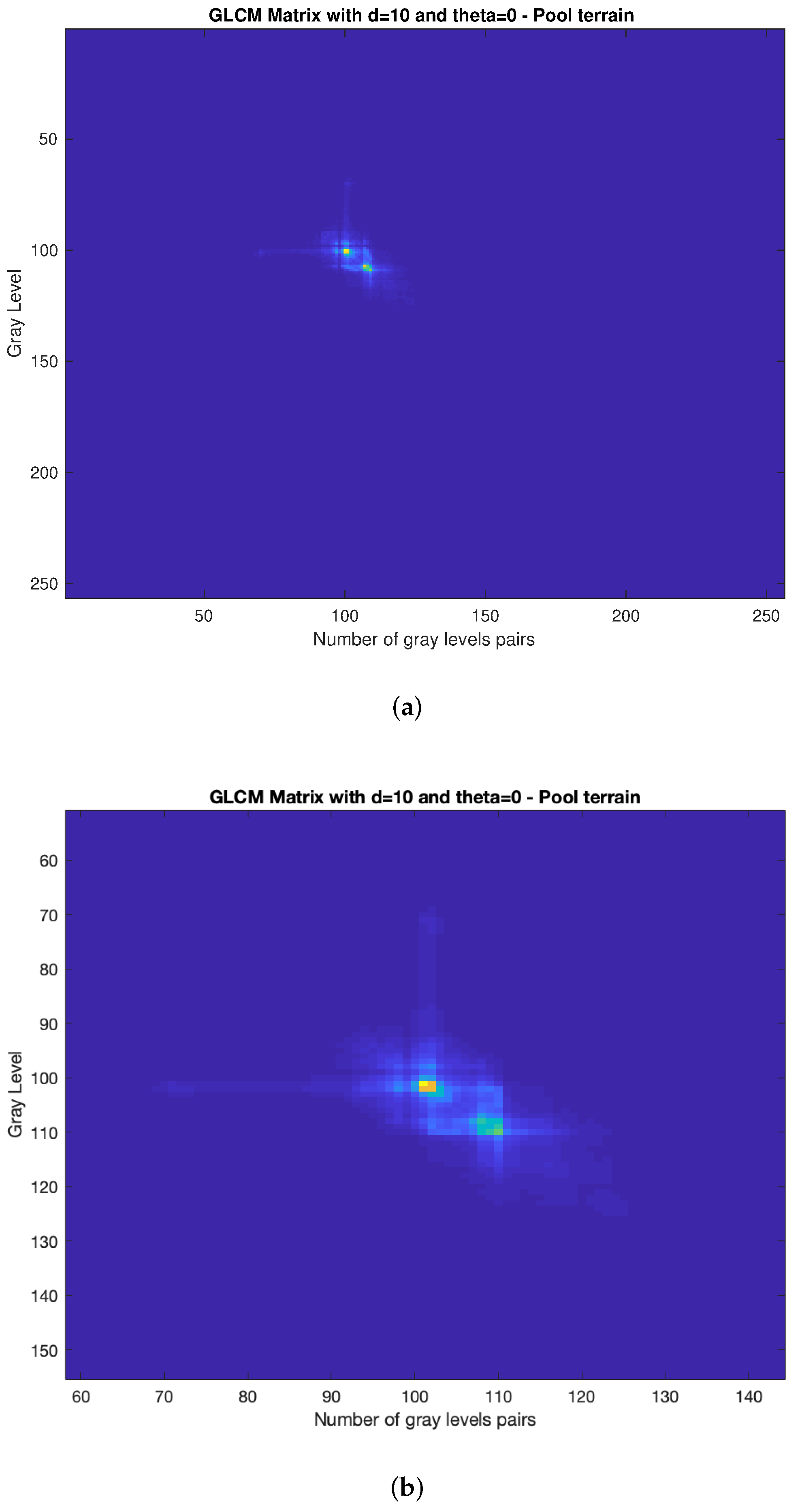
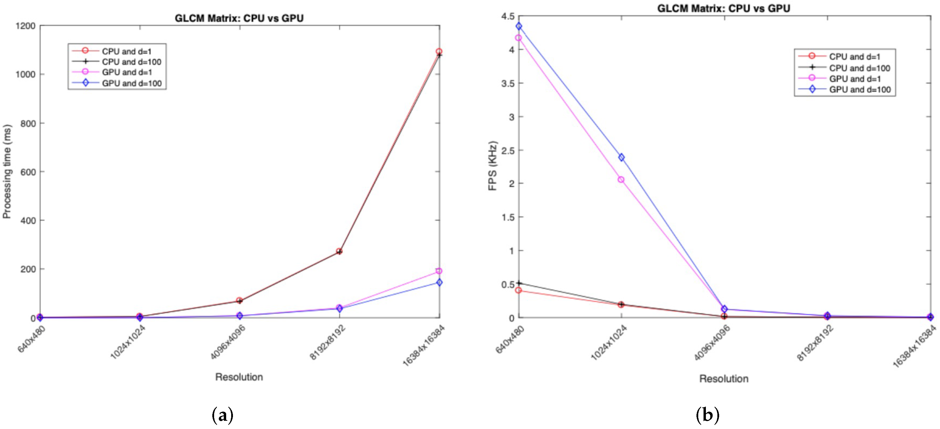
3.3.3. Gray-Level Co-Occurrence Matrix

As explained in Section 2, previous research works have described different terrain classification approaches mainly using static features from RGB images taken onboard of UAVs. This section illustrated the design of a computer vision system to classify terrain types that extracts features from the UAV’s downwash effect known as GLCM. Thus, two main steps were considered:

1.

GLCM mask design;

2.

Calculation of 27 features.

As a first step, it was necessary to create the GLCM N × N matrix. In this paper, the matrix dimensions were 256 × 256 because the input images were defined between 0 and 255 levels (256 gray levels).

In this paper, we chose $d=100$ (offset), $\theta =0$, and a symmetric matrix in order to have a trade-off between noise and system speed. These values were obtained by trial and error.

As it can be seen in Algorithm 1, the initial GLCM matrix was created. For the development of the second stage of the matrix, the transpose matrix $M^T$ was developed using Algorithm 2.

Algorithm 1 GLCM mask design.

$sizeGlcmMask\leftarrow 256$ $glcmArray\left[sizeGlcmMask\right]\left[sizeGlcmMask\right]$ $rows\leftarrow yf$ $cols\leftarrow xf$ $pixelPtrRead\leftarrow imageGray.data$ for$y=yi$ to $rows$ do    for $x=xi$ to $cols-glcmOffset$ do      $i\leftarrow pixelPtrRead(y,x)$      $j\leftarrow pixelPtrRead(y,x+glcmOffset)$      $glcmArray\left[i\right]\left[j\right]$ += 1    end for end for

Algorithm 2 GLCM transpose mask design.

$sizeGlcmMask\leftarrow 256$ $glcmTranspose\left[sizeGlcmMask\right]\left[sizeGlcmMask\right]$ for$y=0$ to $sizeGlcmMask-1$ do    for $x=0$ to $sizeGlcmMask-1$ do      $glcmTranspose\left[x\right]\left[y\right]$ += $glcmArray\left[y\right]\left[x\right]$    end for end for

For the last step in creating the presented algorithm, the symmetric matrix was developed, as shown in Equation (13):

$$M^F=M+M^T$$

(13)

Thus, Algorithm 3 was designed in order to present the final GLCM matrix.

Algorithm 3 GLCM transpose mask design.

for$y=0$ to $sizeGlcmMask-1$ do    for $x=0$ to $sizeGlcmMask-1$ do      $glcmArray\left[y\right]\left[x\right]$ += $glcmTranspose\left[y\right]\left[x\right]$    end for end for

Figure 4 shows an example of water terrain results using the GLCM algorithm.

With the GLCM matrix defined, 26 textural features and 1 intensity color were extracted to classify the terrain. The calculations were conducted according to Equations (14)–():

$$\begin{array}{c}\hfill \begin{array}{cc}\hfill p_{i-j,k}=& \sum _{i=0}^{N-1}\sum _{j=0}^{N-1}p(i,j)ifk=|i-j|k=0,...,N-1\hfill \end{array}\end{array}$$

(14)

$$\begin{array}{c}\hfill \begin{array}{cc}\hfill p_{i-j,k}=& \sum _{i=0}^{N-1}\sum _{j=0}^{N-1}p(i,j)ifk=i+jk=2,...,2N\hfill \end{array}\end{array}$$

(15)

$$\begin{array}{c}\hfill \begin{array}{cc}\hfill p_x\left(i\right)=& \sum _{j=1}^{N}p(i,j)\hfill \end{array}\end{array}$$

(16)

$$\begin{array}{c}\hfill \begin{array}{cc}\hfill p_y\left(j\right)=& \sum _{i=1}^{N}p(i,j)\hfill \end{array}\end{array}$$

(17)

$$\begin{array}{c}\hfill \begin{array}{cc}\hfill HX=& -\sum _{i=1}^N{p}_x\left(i\right)·{log}_2\left(p_x\left(i\right)\right)\hfill \end{array}\end{array}$$

(18)

$$\begin{array}{c}\hfill \begin{array}{cc}\hfill HY=& -\sum _{j=1}^N{p}_y\left(j\right)·{log}_2\left(p_y\left(j\right)\right)\hfill \end{array}\end{array}$$

(19)

$$\begin{array}{c}\hfill \begin{array}{cc}\hfill HXY=& -\sum _{i=1}^N\sum _{j=1}^{N}p(i,j)·{log}_2\left(p(i,j)\right)\hfill \end{array}\end{array}$$

(20)

$$\begin{array}{c}\hfill \begin{array}{cc}\hfill HXY1=& -\sum _{i=1}^N\sum _{j=1}^{N}p(i,j)·{log}_2(p_x\left(i\right)·p_y\left(j\right))\hfill \end{array}\end{array}$$

(21)

$$\begin{array}{c}\hfill \begin{array}{cc}\hfill HXY2=& -\sum _{i=1}^N\sum _{j=1}^N{p}_x\left(i\right)·p_y\left(j\right)·{log}_2(p_x\left(i\right)·p_y\left(j\right))\hfill \end{array}\end{array}$$

(22)

where $p(i,j)={(i,j)}^{th}$ is the entry in a GLCM normalized matrix, and N is the maximum gray intensity level (in this paper, 255). Thus,

Table 1. Calculation of 26 textural features.

Feature	Computation
Auto-correlation	${\sum }_{i=0}^{N-1}{\sum }_{j=0}^{N-1}ijp(i,j)$
Cluster Prominence	${\sum }_{i=0}^{N-1}{\sum }_{j=0}^{N-1}{((i-\mu )+(j-\mu ))}^{4}p(i,j)$
Cluster Shade	${\sum }_{i=0}^{N-1}{\sum }_{j=0}^{N-1}{((i-\mu )+(j-\mu ))}^{3}p(i,j)$
Cluster Tendency	${\sum }_{i=0}^{N-1}{\sum }_{j=0}^{N-1}{((i-\mu )+(j-\mu ))}^{2}p(i,j)$
Contrast	${\sum }_{i=0}^{N-1}{\sum }_{j=0}^{N-1}{|i-j|}^2·p(i,j)$
Correlation	${\sum }_{i=0}^{N-1}{\sum }_{j=0}^{N-1}\frac{(i-{\mu }_x)(j-{\mu }_y)·p(i,j)}{{\sigma }_x·{\sigma }_y}$
Difference Average	${\sum }_{k=0}^{N-1}k·p_{i-j,k}$
Difference Entropy	$-{\sum }_{k=0}^{N-1}{p}_{i-j,k}·{log}_2\left(p_{i-j,k}\right)$
Difference Variance	${\sum }_{k=0}^{N-1}{(k-DifferenceAverage)}^2·p_{i-j,k}$
Energy	${\sum }_{i=0}^{N-1}{\sum }_{j=0}^{N-1}p{(i,j)}^2$
Entropy	$-{\sum }_{i=0}^{N-1}{\sum }_{j=0}^{N-1}p(i,j)·{log}_2\left(p(i,j)\right)$
Homogeneity	${\sum }_{i=0}^{N-1}{\sum }_{j=0}^{N-1}\frac{p(i,j)}{1+|i-j|}$
Homogeneity Moment	${\sum }_{i=0}^{N-1}{\sum }_{j=0}^{N-1}\frac{p(i,j)}{{1+|i-j|}^2}$
Homogeneity Moment Normalized	${\sum }_{i=0}^{N-1}{\sum }_{j=0}^{N-1}\frac{p(i,j)}{1+\frac{{|i-j|}^2}{N^2}}$
Homogeneity Normalized	${\sum }_{i=0}^{N-1}{\sum }_{j=0}^{N-1}\frac{p(i,j)}{1+\frac{|i-j|}{N}}$
Inverse Variance	${\sum }_{i=0}^{N-1}{\sum }_{j=0}^{N-1}\frac{p(i,j)}{{1+|i-j|}^2},i\ne j$
Informational Measure of Correlation 1	$\frac{HXY-HXY1}{max(HX,HY)}$
Informational Measure of Correlation 2	$\sqrt{1-e^{-2·(HXY2-HXY)}}$
Joint Average	${\sum }_{i=0}^{N-1}{\sum }_{j=0}^{N-1}ip(i,j)$
Joint Maximum	$max\left(p\right(i,j\left)\right)$
Kurtosis	$\frac{\frac{1}{N}·{\sum }_{i=0}^{N-1}{(x_i-{\mu }_x)}^4}{{\left(\frac{1}{N}·{\sum }_{i=0}^{N-1}{(x_i-{\mu }_x)}^2\right)}^2}$
Skewness	$\frac{{\sum }_{i=0}^{N-1}{(x_i-{\mu }_x)}^3}{N·{\sigma }_x^3}$
Sum Average	${\sum }_{k=2}^{2N}k·p_{i+j,k}$
Sum Entropy	$-{\sum }_{k=2}^{2N}{p}_{i+j,k}·{log}_2\left(p_{i+j,k}\right)$
Sum Variance	${\sum }_{k=2}^{2N}{(k-SumAverage)}^2·p_{i+j,k}$
Variance	${\sum }_{i=0}^{N-1}{\sum }_{j=0}^{N-1}{(i-\mu )}^2·p(i,j)$

shows the total texture and color features used in this section to classify the terrain under study.

where the following apply:

• Auto-correlation: A measure of the magnitude of the fineness and coarseness of texture;
• Joint Average: The gray-level weighted sum of joint probabilities;
• Cluster Prominence: It measures the GLCM asymmetry; higher values indicate more asymmetry, whereas lower values indicate the peak of the distribution centered around the mean;
• Cluster Shade: It measures the skewness of the GLCM matrix; a higher value indicates asymmetry;
• Cluster Tendency: It measures the heterogeneity that places higher weights on neighboring intensity level pairs that deviate more from the mean;
• Contrast: It is used to return the intensity level between a pixel and its neighbor throughout the entire image;
• Correlation: This method is important to define how a pixel is correlated with its neighbor throughout the entire image;
• Difference Average: It measures the mean of the gray-level difference distribution of the current frame;
• Difference Entropy: It measures the disorder related to the gray-level difference distribution of the current frame;
• Entropy: This feature measures the randomness of the intensity distribution. The greater the information’s heterogeneity in an image, the greater the entropy value is; however, when homogeneity increases, the entropy tends to 0;
• Homogeneity: Known as Inverse Difference Moment, this equation returns 1 when the GLCM is uniform (diagonal matrix);
• Homogeneity Moment: It measures the local homogeneity of an image; the result is a low Homogeneity Moment value for heterogeneous images and a relatively higher value for homogeneous images;
• Homogeneity Moment Normalized: It has the same goal as the Homogeneity Moment, but the neighboring intensity values are normalized by the highest intensity value with a power of 2;
• Homogeneity Normalized: It has the same goal as the Homogeneity Moment but the neighboring intensity values are normalized by the highest intensity value;
• Sum Average: It measures the mean of the intensity level sum distribution of the current frame;
• Sum Entropy: It measures the disorder related to the intensity value sum distribution of the current frame;
• Sum Variance: It measures the dispersion of the intensity number sum distribution of the current frame;
• Variance: It represents the measure of the dispersion of the values around the mean.

To provide more information to the system about the terrain color under study, the HSV method was used, and it is explained in this section.

Figure 5 shows one way to represent this color model. The Hue component represents a distinct color, represented by an angle and thus with values between 0 and 360 (values in degrees; the range can also be represented in radians [0, 2$\pi$] or values in the range [0, 1] if the RGB channels are divided by 255 (max byte value)). The Saturation and Value components usually correspond to the range [0, 255] or [0, 1]. The lower the saturation value is, the grayer the image becomes. Regarding Value, the higher its value is, the brighter the image is.

Thus, for RGB-to-HSV conversion images, the following Equations (23)–(25) were used, where R, G, and B correspond to the red, green, and blue (respectively) pixel components; Min is the minimum of the three channels (Min(R,G,B)); and Max is also the maximum value of the three channels (Max(R,G,B)):

$$Hue=\left\{\begin{array}{c}\begin{array}{ccc}\hfill & 0\hfill & \hfill ifMax=Min\\ \hfill & 60·\frac{G-B}{Max-Min}\hfill & \hfill ifMax=R\&G\ge B\\ \hfill & 60·\frac{G-B}{Max-Min}+360\hfill & \hfill ifMax=R\&G<B\\ \hfill & 60·\frac{B-R}{Max-Min}+120\hfill & \hfill ifMax=G\\ \hfill & 60·\frac{R-G}{Max-Min}+120\hfill & \hfill ifMax=B\end{array}\hfill \end{array}\right.$$

(23)

$$Saturarion=\frac{Max-Min}{Max}$$

(24)

$$Value=Max$$

(25)

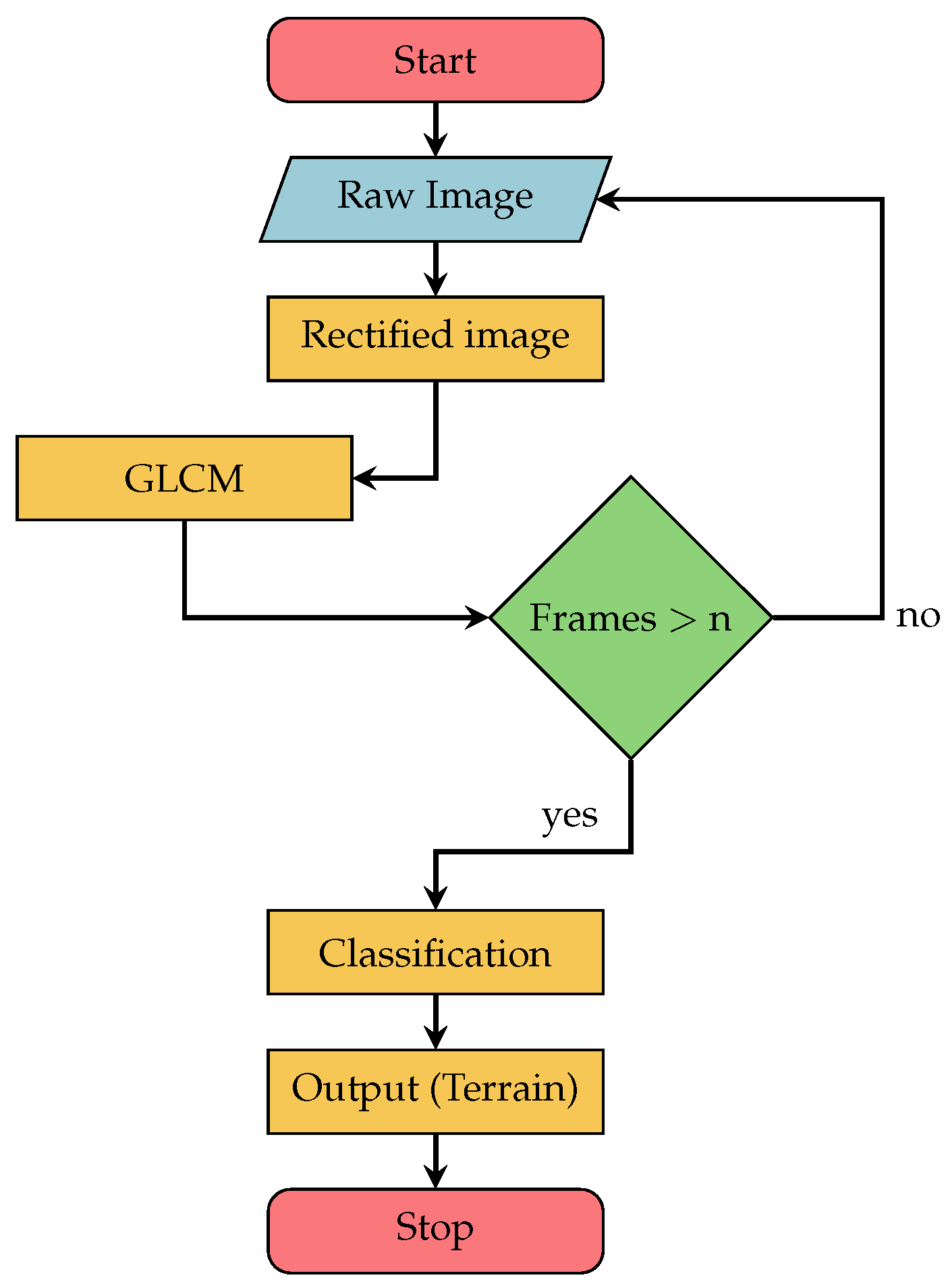
3.4. System Architecture

Thus, after explaining the features used in this section, in order to explain how the GLCM and PSO algorithms were applied in this paper, the proposed system model for terrain classification is presented in Figure 6.

From the proposed system model in Figure 6, it is possible to visualize five main processes identified in the architecture, namely:

• Raw Image: The images obtained by the RGB camera have a resolution of 640 by 480 pixels; after obtaining these images, the RGB information is sent to the next layer;
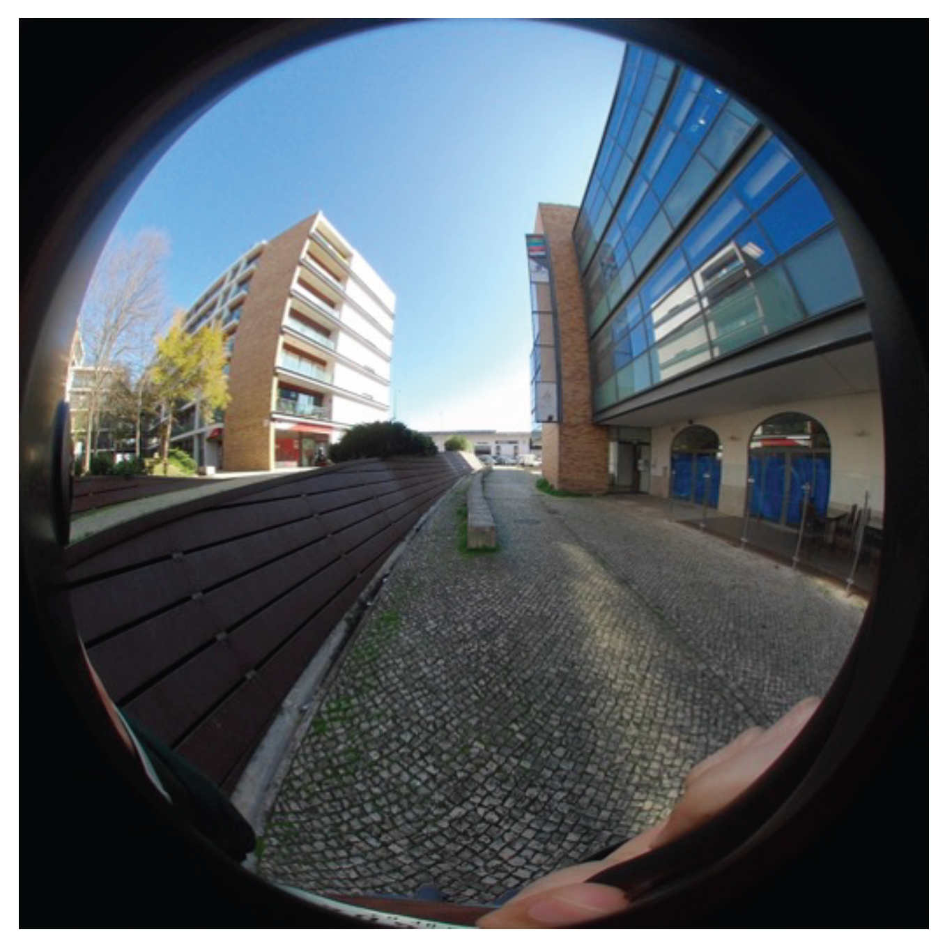
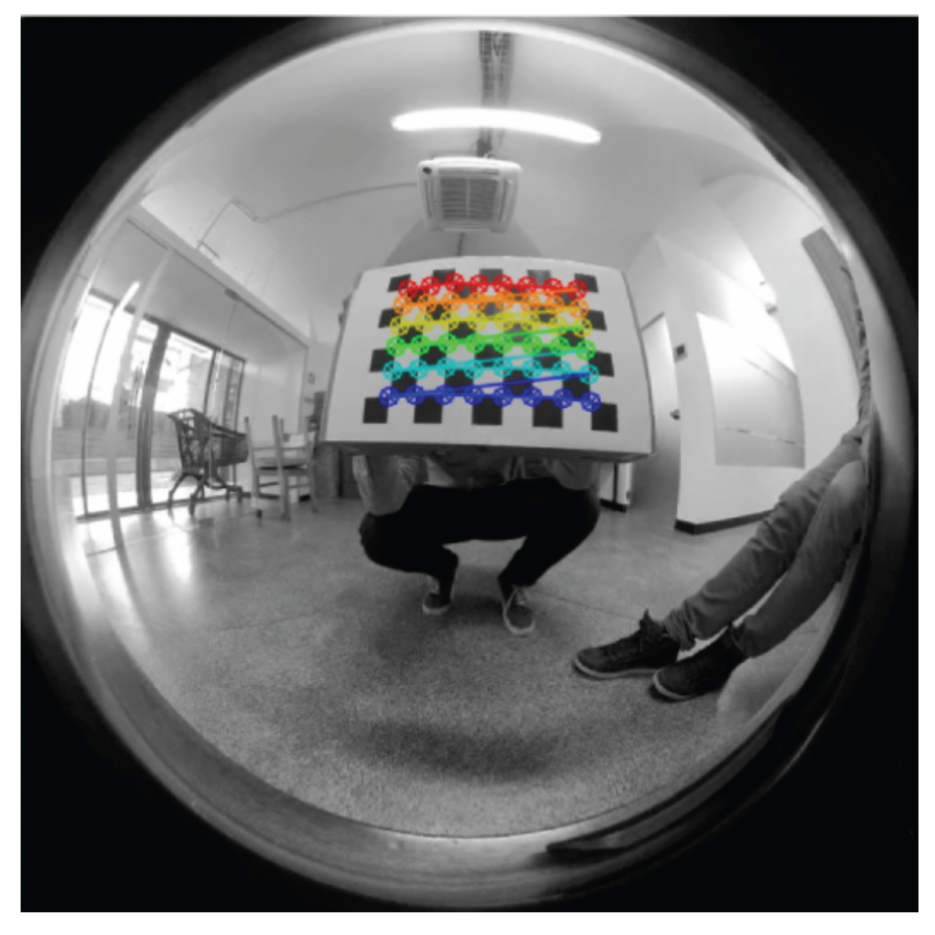
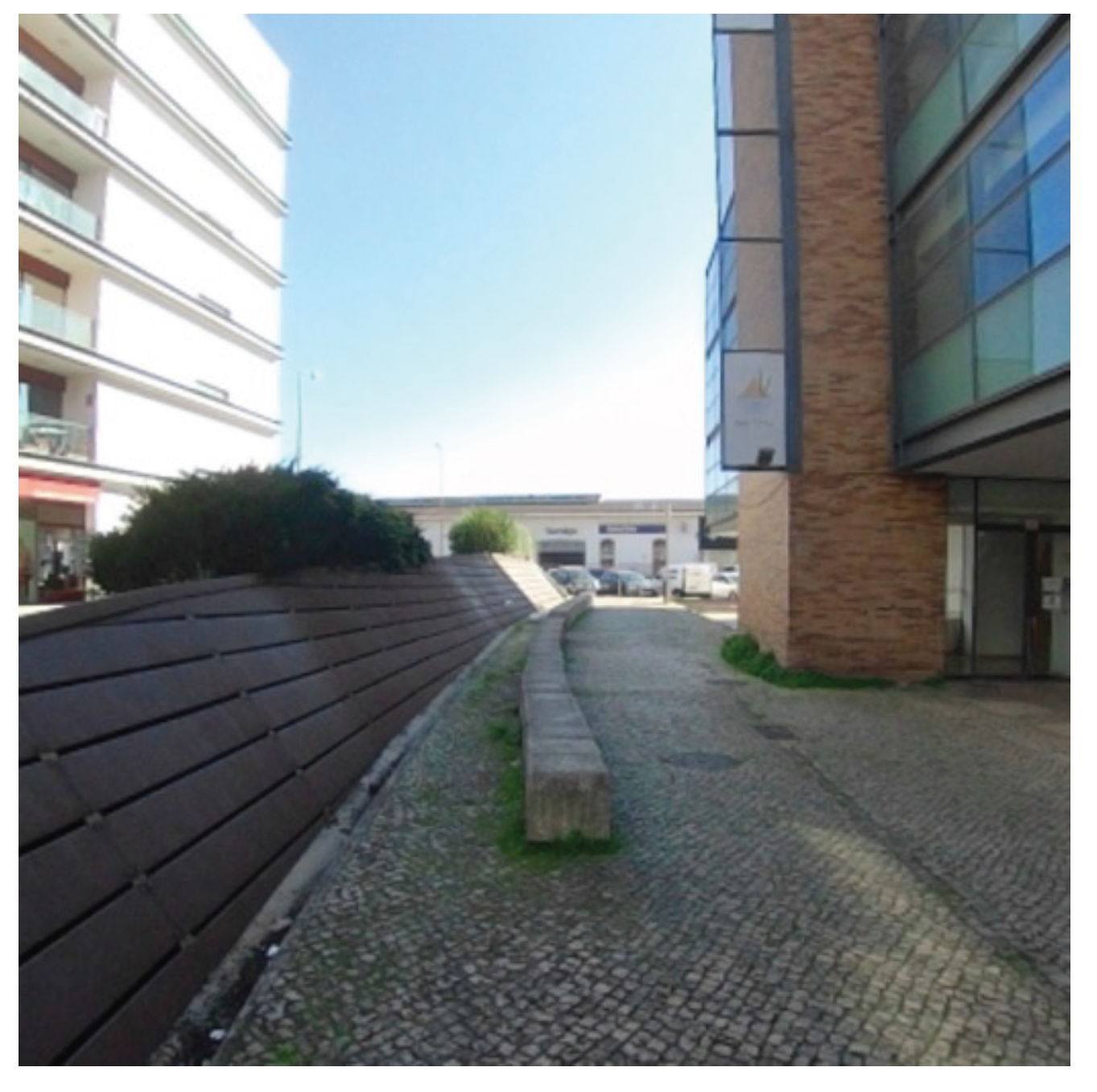
• Rectified Image: To work with all RGB cameras with the same proposed algorithm, it is necessary to calibrate the cameras; Section 3.5 explains how to calibrate these RGB cameras;
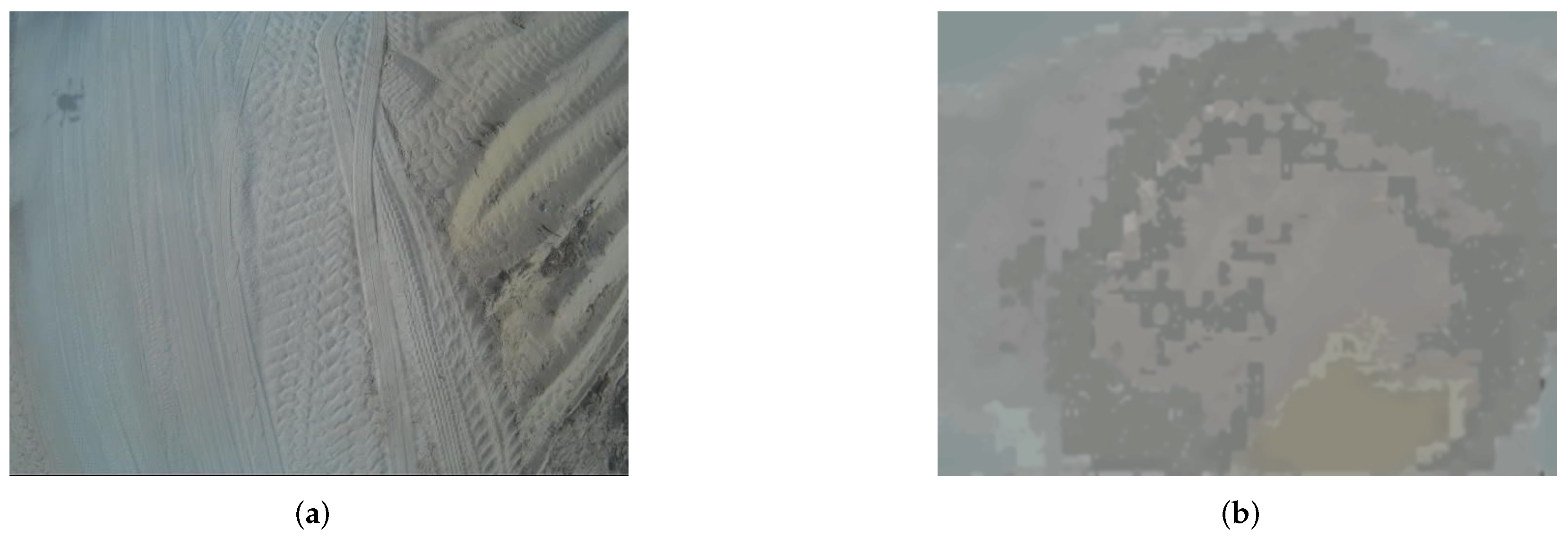
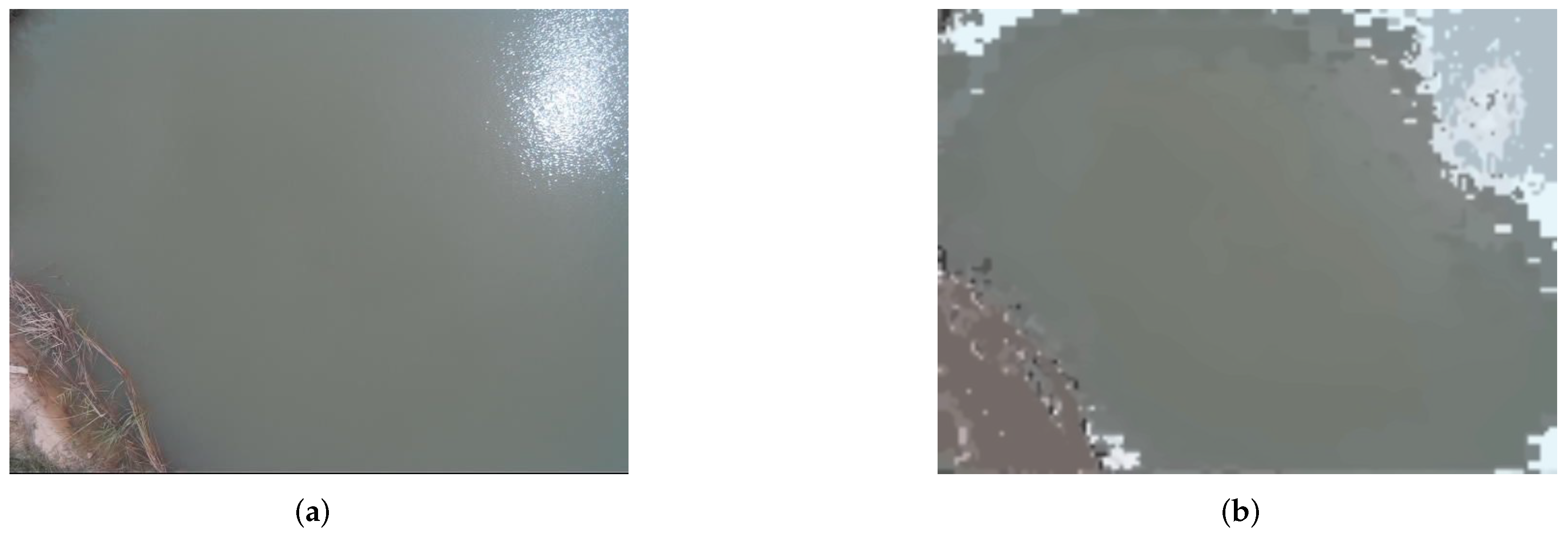
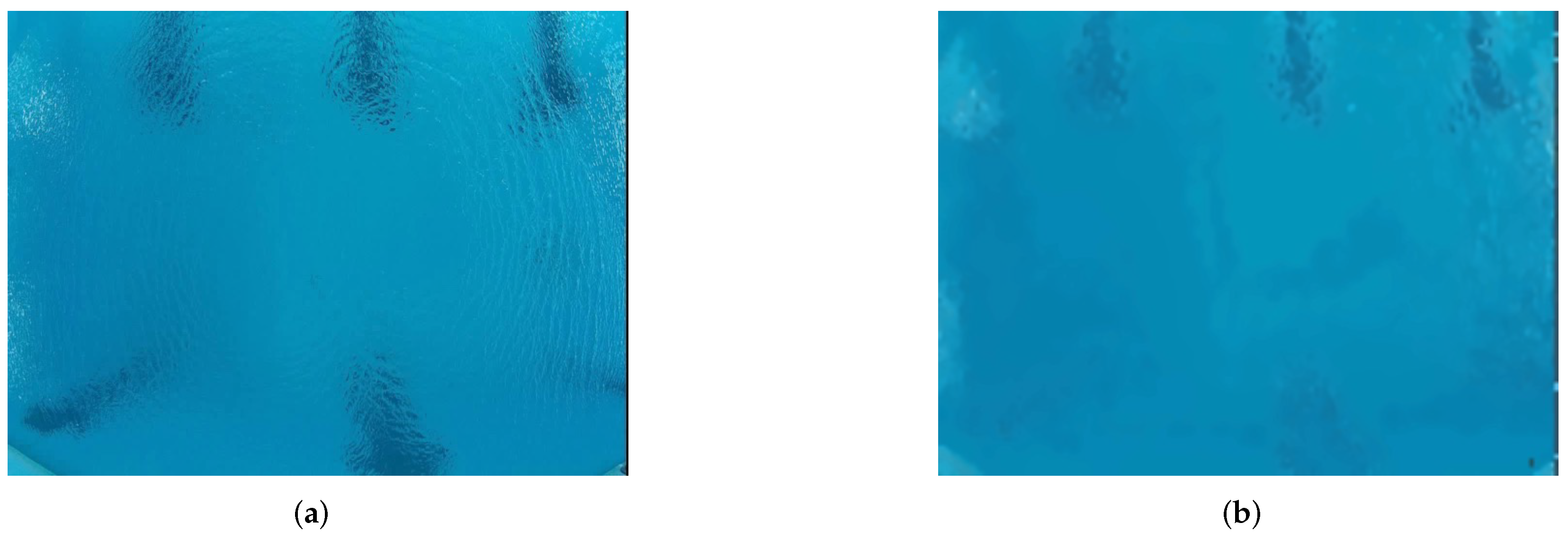
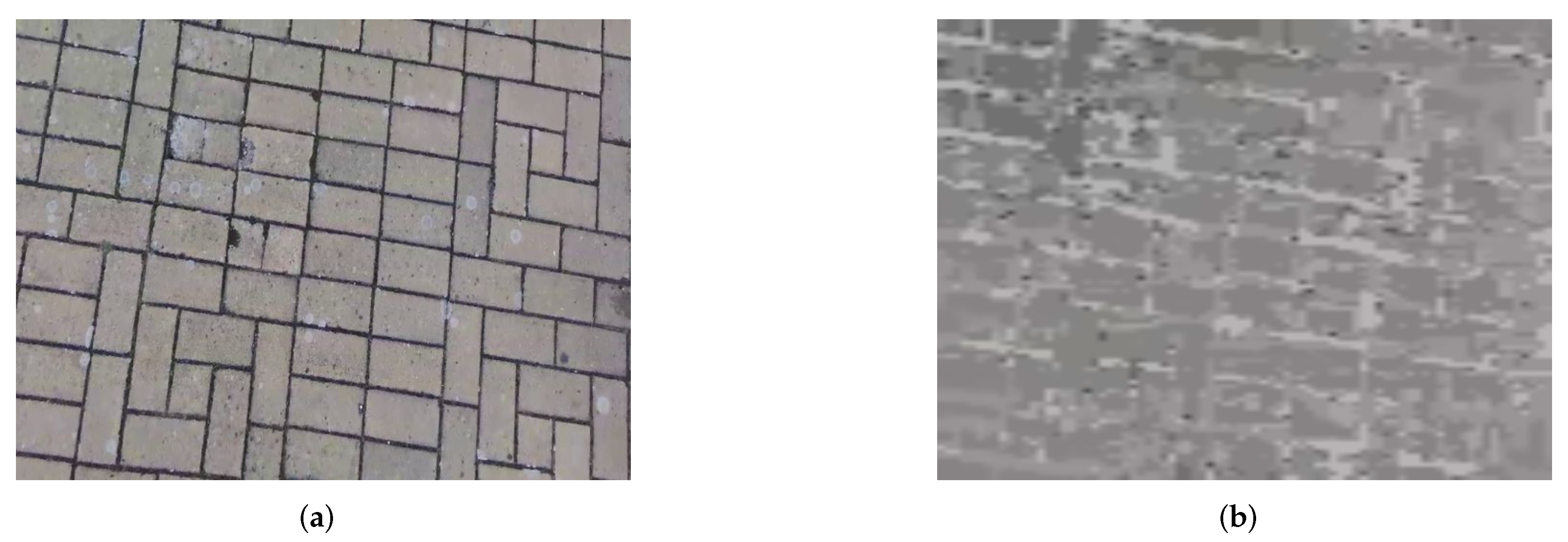
• Swarm Optimization: This layer is responsible for segmenting the terrain type captured by the RGB camera to be sent to the next layer (GLCM);
• Gray-Level Co-Occurrence Matrix: When receiving the segmented images from the PSO layer, this layer is responsible for transforming a segmented image into a GLCM matrix, where the features in Section 3.3.3 are calculated;
• Classification: The outputs generated by the GLCM phases are turned into inputs for a neural network (NN), which classifies the terrain. In this section, a Multilayer Perceptron (MLP) architecture is used. The neural network inputs are the output values from GLCM phase. The neural network model consists of three layers: the hidden layer contains 10 neurons, whereas the third layer corresponds to the system output and has the number of possible terrain outputs under study in this paper. Each neuron is activated by a sigmoidal function; they present a fully connected feed-forward neural network. During the training stage, 70% of the total data are used for training, 15% for testing, and 15% for validation.

Given the system model explanation, in this section, four different terrain types (rock, vegetation, sand, water, and asphalt) are analyzed. The following six figures (Figure 7, Figure 8, Figure 9, Figure 10, Figure 11 and Figure 12) show the results of the PSO of each terrain under study in this work. Figures (a) show the raw images and Figures (b) present the clustering results.

3.5. Camera Calibration

An RGB camera can be used to obtain various data from a given environment, such as length, distance, size, and others. Data may need more than one sensor to be collected. For this, it is necessary to know the camera’s calibration parameters [39].

As seen in Figure 13, the camera used had a distortion known as fish-eye. Such distortion allows a greater opening to be obtained; however, the size of the objects is not coherent. Therefore, the camera was subjected to a calibration process (http://wiki.ros.org/camera_calibration (accessed on 13 March 2022)) using a tool available in ROS.

The calibration uses a table according to the method proposed in [40], where planar chessboard patterns with known dimensions are presented. The planar chessboard is presented at different angles and positions for computing the relationship among the distances between each point, as can be seen in Figure 14.

After calibration, a file is generated containing the camera parameters, which can be used to remove distortion and compute the images to obtain scene data. The image without fish-eye distortion through the collected parameters can be seen in Figure 15.

4. Empirical Part and Discussion of Results

To test the combination of PSO and GLCM, the 27 features studied in Section 3.3.3 were calculated and computed; then, they were applied to each dataset image (see Table 1). The results of the whole set of studied frames were analyzed, and a combination of 12 of 27 features was selected by the authors. The selected combination of features was: 1—Variance with IMC1; 2—Correlation with Joint Average; 3—Variance with Difference Entropy; 4—Homogeneity with Variance; 5—Entropy with Variance; 6—Variance with IMC2; 7—Sum Average with Difference Entropy; 8—Sum Average with IMC1; 9—Sum Average with IMC2; 10—Auto-Correlation with IMC1; 11—Auto-Correlation with IMC2; 12—Joint Average with IMC2.

As can be seen from the selected feature enumeration, it is possible to conclude that the impact of the features was the following:

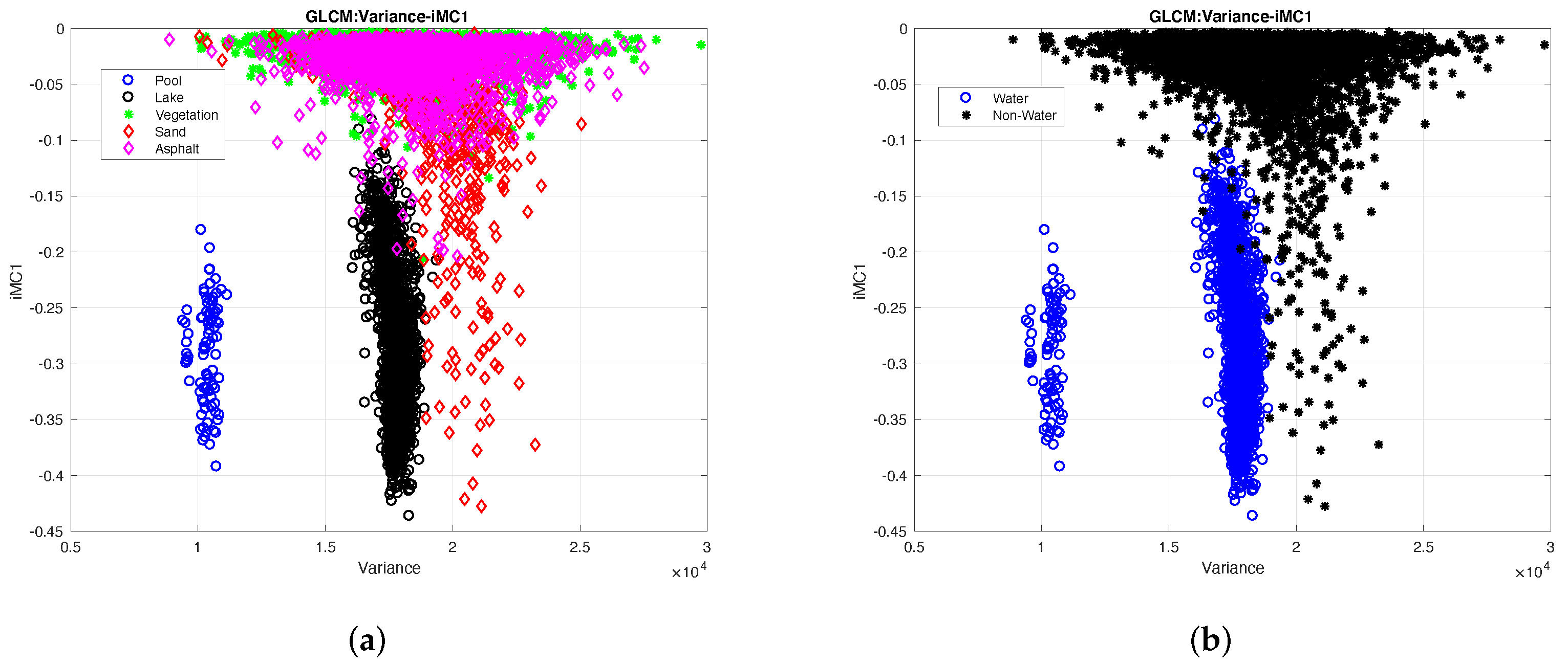
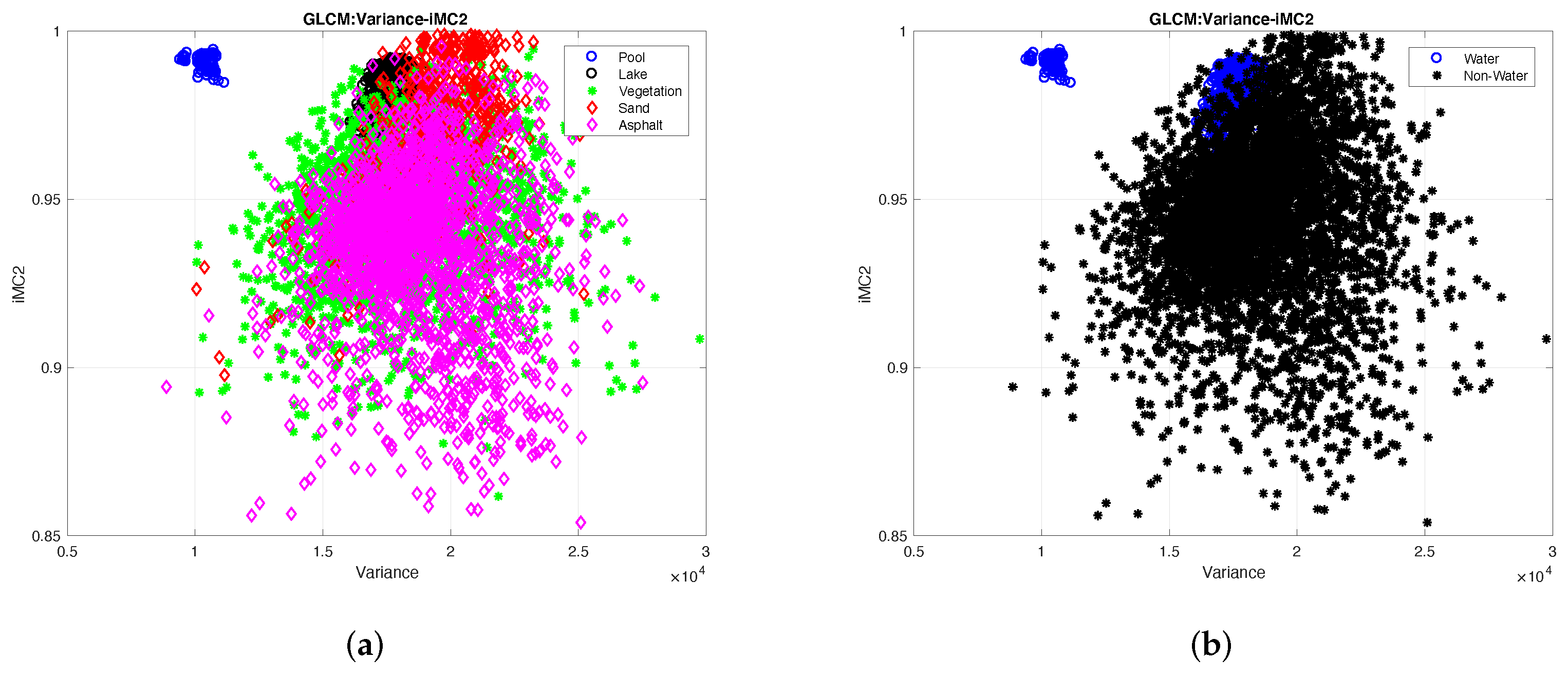
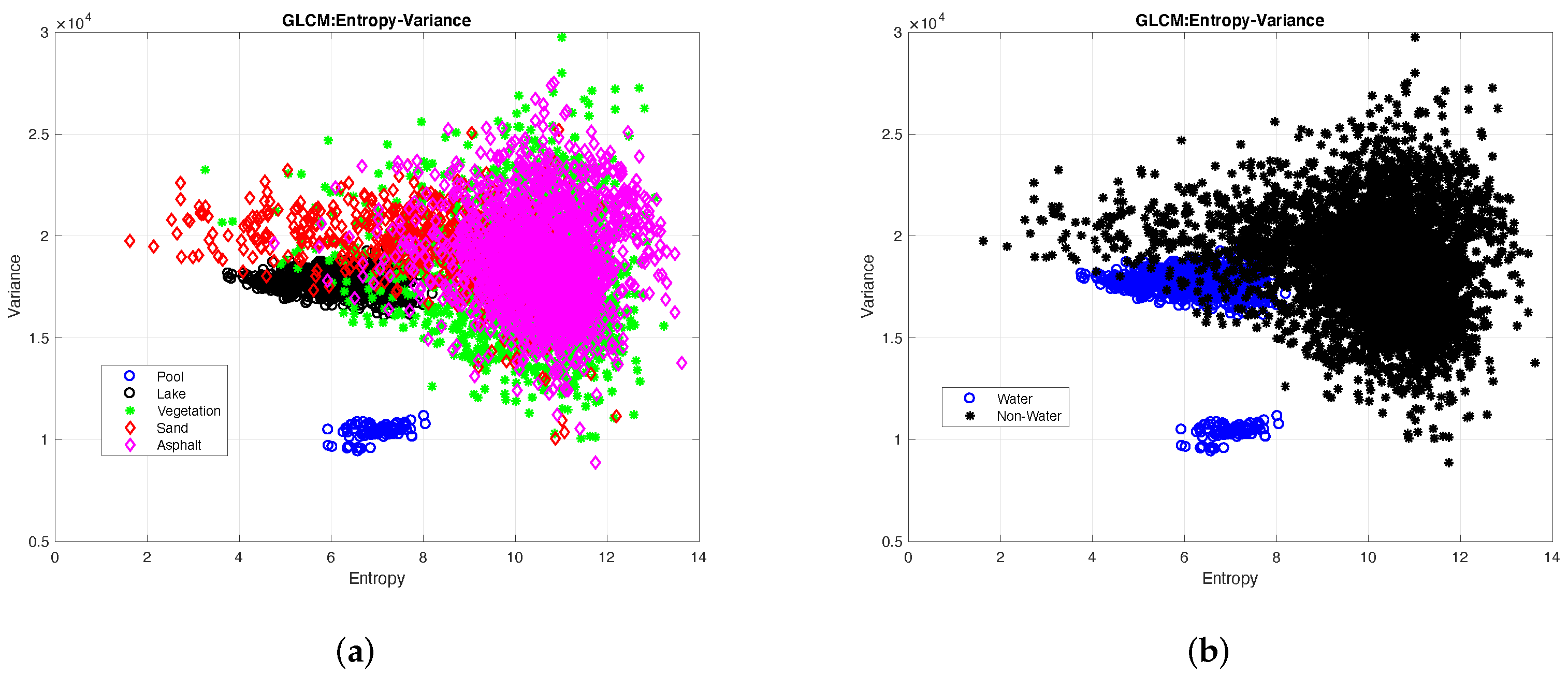
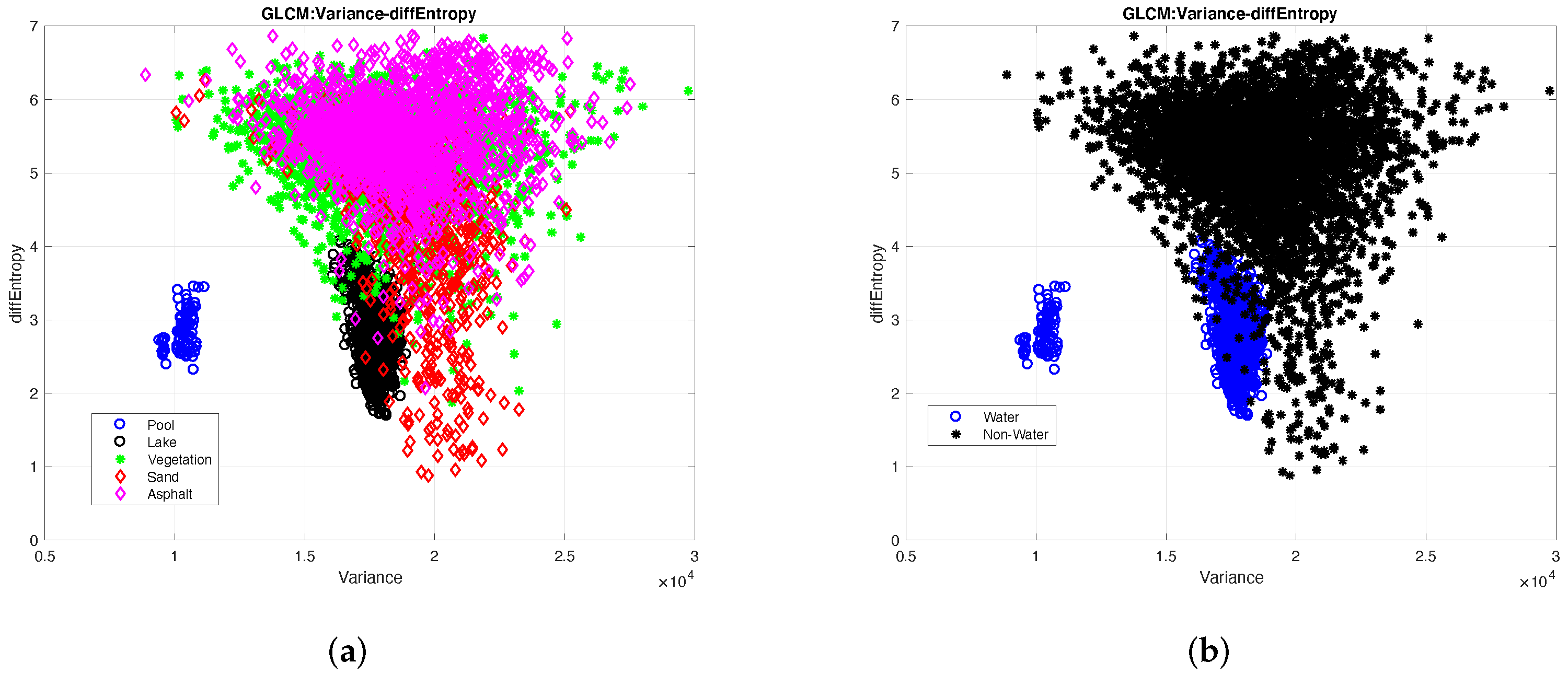
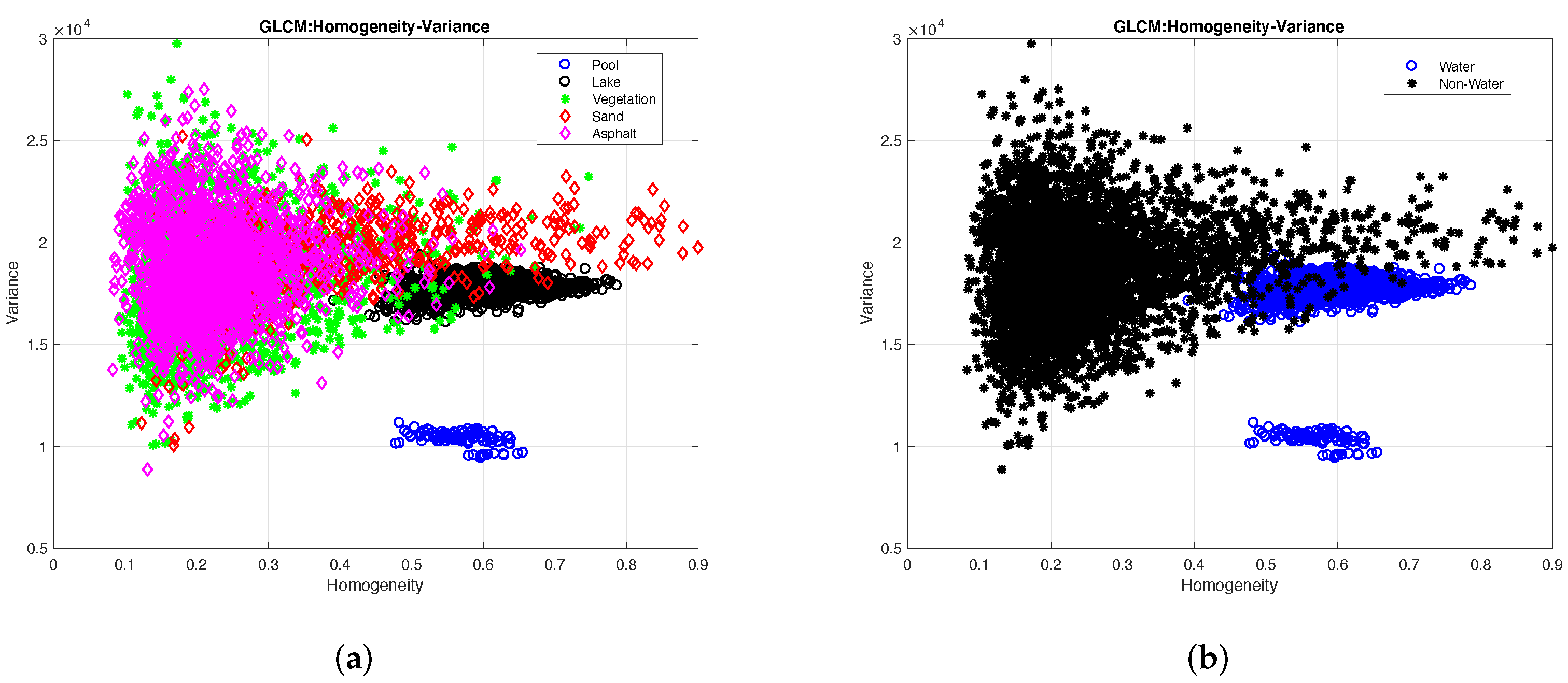
• Variance—41.67% of impact;
• IMC2—33.33% of impact;
• IMC1—25.00% of impact;
• Sum Average—25.00% of impact;
• Joint Average—16.67% of impact;
• Difference Entropy—16.67% of impact;
• Auto-Correlation—16.67% of impact;
• Correlation—8.33% of impact;
• Entropy—8.33% of impact;
• Homogeneity—8.33% of impact.

Since the Variance feature was used in more than 41% of cases, Figure 16, Figure 17, Figure 18, Figure 19 and Figure 20 show the results obtained from comparing Variance to IMC1, IMC2, Entropy, Difference Entropy, Correlation and Homogeneity, for the whole dataset.

In Figures (a), the water terrain type is represented by black (pool) and blue (lake); green represents the vegetation-type terrain; sand-type terrain is represented by pink; red represents the asphalt-type terrain. In Figures (b), the water-type terrain is represented by blue (pool and lake), and black represents the non-water-type terrain.

Using the downwash effect caused by the UAV, the output results are more compact (as it makes the system much more stable), as can be observed in Figure 21. Using the proposed dataset and training the NN, we obtained 87.4% accuracy on the training set and 88.7% on the test dataset.

Since the processing time is an important factor in terrain classification, the authors of this paper also studied the GPU capabilities in the GLCM matrix design using the CUDA framework. To build the GLCM matrix, the pixel values are used as the coordinates of the matrix itself. Therefore, if one or more threads try to write in the same coordinates of the GLCM matrix, an undefined result occurs. To solve this, atomic operations are needed to serialize operations and ensure that the latest value is read. Hence, whenever there is more than one thread writing in the same position in the GLCM matrix, priority is given to the first thread, etc. This solution has an advantage and a disadvantage:

• Advantage—The atomic operation ensures that there are no undefined values and the final result is correct;
• Disadvantage—The disadvantage centers on the fact that parallelism gets lost in these situations of having to write in the same memory; in this way, the processing time is reduced.

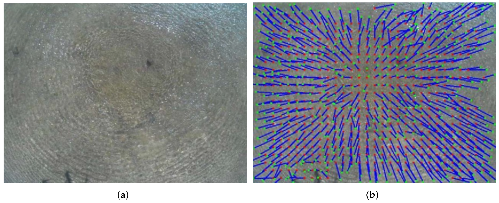
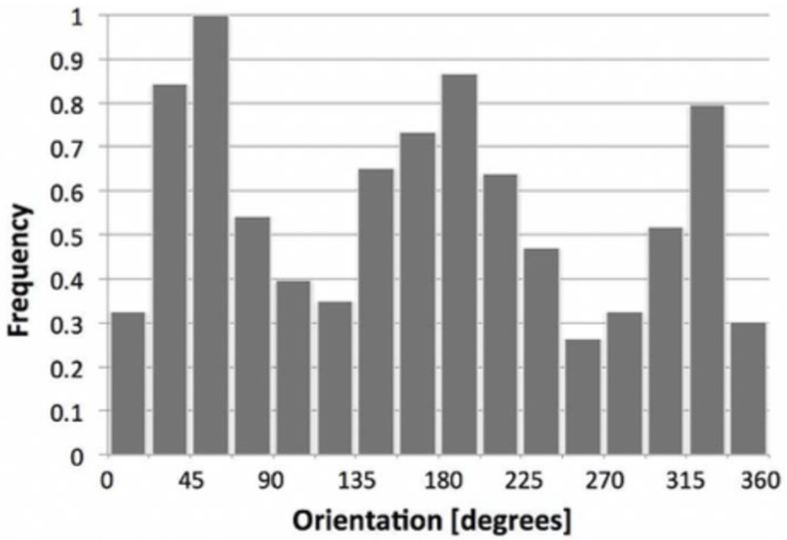
To verify this effect in detail (several threads writing in the same memory at the same time), the CUDA algorithm ran on two images, as shown in Figure 22, and the GLCM matrix processing time in both figures was registered. With the same image dimensions (width = 640 and height = 480) and the same number of blocks and threads in each block, the two following statements were drawn: The processing using CUDA programming in Figure 22a was 0.230 ms, while in Figure 22b, it was 0.195 ms; therefore, in Figure 22b, the processing time was 1.18 times faster than in Figure 22a. These results are due to the fact that in water-type terrains, the pixel values are closer to each other (being a much more homogeneous image) than in vegetation-type terrains, where there is a greater diversity of pixel colors. There is a greater probability that the threads write in the same memory position when studying water-type terrains and, consequently, suffer from poorer processing-time performance.

The difference in processing time when programmed in the CPU and GPU concerning the GLCM matrix was also studied in detail. Figure 22a was used as a case study, and the difference was analyzed for different resolutions, maintaining the same number of threads in each block and a ratio of grid blocks of Width/threads in X and Height/thread in Y.

Table 2. Processing time for different resolutions and GLCM distance parameters.

Width	Height	Distance	CPU Working Time (ms)	GPU Working Time (ms)	Acceleration
640	480	1	2.491	0.240	10.379
		100	1.944	0.230	8.452
1024	1024	1	5.408	0.488	11.082
		100	5.067	0.418	12.122
4096	4096	1	69.617	8.194	8.496
		100	67.392	7.965	8.461
8192	8192	1	271.039	40.576	6.680
		100	269.634	36.995	7.288
16,384	16,384	1	1092.070	190.093	5.745
		100	1078.060	145.195	7.425

and Figure 23 show the results obtained.

From Table 2 and Figure 23a,b it is possible to conclude that using the capacities of the GPU always resulted in a better processing time regardless of the image size and the distance parameter (distance between pixels to form GLCM matrix cell) for the developed GLCM matrix.

As illustrated in Figure 23a,b, it is possible to make some important observations. Regarding resolution, as it increased, the processing time also increased when programming using the CPU and GPU, mainly at the 16,384 × 16,384 resolution, where the processing time using the CPU was approximately 1 s and 0.190 s using the GPU (with the distance parameter equal to 1). It is also possible to observe that as the resolution of the image increased, the processing time increased exponentially both in the CPU and GPU. It is also known that, generally, the higher the resolution of the image is, the greater the accuracy of terrain classification is (it is possible to obtain many more data in the same image). It is necessary to have a trade-off between system accuracy and algorithm processing time. In terms of the choice between CPU and GPU, the GPU is preferred because of its ability to process the video stream in real-time, which is vital in the context of UAV monitoring.

Based on the obtained accuracy results, the authors conducted a comparison with the existing methods of terrain classification.

Table 3. Terrain classification—accuracy comparison.

Method	Terrain Recognition Accuracy (%)
GLCM [45]	81.90
GLCM [46]	86.60
LBP [46]	90.48
Depth Texture Features [47]	92.30
LiDAR [48]	75.55
Multispectral Camera [49]	80.00
Hyperspectral Camera [50]	81.18
Normalized Color [51]	67.00
HOG [52]	86.54
Voronoi [53]	82.30
LBP [54]	96.90
LTP [54]	98.10
LATP [54]	97.20
Gabor [55]	96.11
Optical Flow [41]	87.00
CNNs [56]	86.25
RNN [57]	83.49
PSO + GLCM	88.70

shows the general overview of terrain recognition accuracy for the existing methods and the authors’ algorithm.

Some of the works researched used the optical flow concept to classify terrains [41,42,43]. Until now, without counting the articles published by the authors of this paper, only one recent publication [41] used this concept for terrain classification. The work [41] used the optical flow concept to extract the dynamic part of an image using the Lucas–Kanade method [44] from an onboard RGB camera, as can be seen in Figure 24.

As can be seen from Figure 25, the authors stated that the downwash effect caused by UAVs on water-type terrains gives rise to a circular motion in which the flows detected by the optical flow start from the center and point outwards.

However, the algorithm proposed by the authors in [41] has two crucial points:

1.

Robustness of the algorithm—Since in water-type terrains movement is circular, it is natural that there is a dispersion at all angles of the captured image; however, if the center of the downwash is not in the center of the image, this dispersion may not occur at all angles in a water-type terrain. In this way, the authors may erroneously conclude that they are not on water-type terrain when, apparently, they are; consequently, the drone would land and damage its hardware;

2.

Processing time—The significantly long algorithm processing time is an issue, since it needs at least four seconds to classify whether the terrain under study is water-type or not, which means that the UAV needs to stand still for at least four seconds to classify which type of terrain it is flying over.

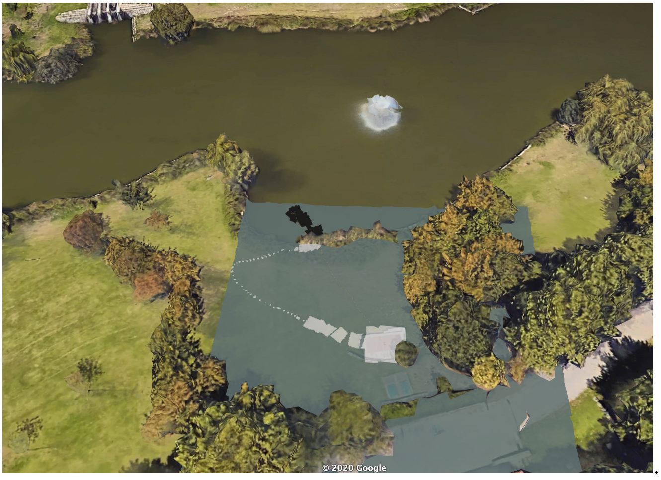
The developed terrain recognition system showed a higher recognition accuracy than the majority of the reviewed methods. One of the key features of the elaborated method is the focus on the image-quality improvement—PSO denoises the raw image and at the same time stores the main texture features. This is vital in the field of UAV monitoring, as the image quality can be impacted by bad weather conditions, illumination issues, etc. In addition, the use of downwash forms more significant features for further terrain-type recognition.

In addition to the visible band (RGB), there are also bands with other frequencies that are used in terrain classification [58,59]. The cameras that use these bands are usually thermal (flir cameras) and multispectral cameras (for example, Micasense RedEdge), as shown in Figure 26.

From the images obtained by the cameras presented in Figure 26, the authors, after aligning the lenses from the red band, used five multispectral indices (NDVI, ENDVI RDVI, MSAVI, and SR) to classify four different terrain types: water, vegetation, sand, and rocks [59]. However, despite the good accuracy of the system proposed by the authors, detecting various types of terrain when the height is higher than 60 m can mean a loss of resolution when classified. Another disadvantage is that shadows can be confused with water-type terrains, due to the fact that water has low values in the NIR and Red-Edge bands.

5. Mapping

After the classification of terrain types (water and non-water), it is necessary to georeference the results obtained by the NN. Using the ROS framework, it is possible to build a dynamic map where all the information obtained by the neural network is allocated. Therefore, in order to validate the dynamic mapping algorithm, a flight test was carried out in Parque da Paz, Portugal. In this test, the UAV performed a mission where it flew over water-type terrain (lake) and non-water-type terrain (vegetation), as shown in Figure 27.

As the UAV flew over different types of terrain, it sent the images via Wi-Fi (using the ROS framework) to the machine responsible for running the algorithms for terrain classification. When the result of each classification was generated, a dynamic map was created as follows:

1.

Black: It represents the water-type terrain;

2.

White: It represents the non-water-type terrain;

3.

Gray: It represents the unknown-type terrain.

Figure 28 shows the georeferenced map results. It is possible to conclude that the proposed algorithm was able to correctly georeference the outputs generated from each image from the UAV. It should be noted that there were different sizes in the generated output due to the different altitudes at which the UAV flew during the mission. It should also be noted that there were certain gaps in each generated output due to the lower UAV GPS resolution.

6. Conclusions

6.1. Results

A computer vision system for classifying terrain types was elaborated. It includes preprocessing by means of PSO, GLCM feature extraction, and a feed-forward neural network.

PSO provides an opportunity for denoising and unifying the images regardless of shooting and weather conditions. An algorithm was developed that consists of preprocessing, feature extraction, and classification. It is capable of recognizing the following different terrain types based on UAV downwash: water, vegetation, asphalt, and sand.

The key features of the developed method are:

• Focus on the preprocessing stage via PSO, which contributes to the recognition-accuracy improvement and can be useful for the systems that are used in a dynamic environment and operate in changing conditions;
• The downwash effect is taken as a base in terrain-type recognition that forms significant features to provide high classification accuracy.

Prospectively, the opportunity of terrain-type classification can contribute to the geolocation determination and self-positioning that could be useful in different spheres of life: monitoring, production, construction, transportation, etc.

6.2. Future Work

Despite the high recognition accuracy obtained, there are several areas in which improvements are foreseen. We plan to further investigate the following topics:

• Perform a more in-depth study on changing the environment colors and improving the robustness of the algorithm. One of the method’s limitations is that a color variation could influence the results with false positives/negatives; although the dynamic texture does not suffer much from these changes, due to the similarity in the way the terrain moves, this could highly affect the static texture;
• Since the algorithm was designed for a UAV flying at an altitude of between one and two meters, it is likely that at this altitude, the UAV may collide with objects in the environment. One of the authors of this paper developed an algorithm [60] to avoid obstacles from images taken from a depth camera; however, currently, it only works with static objects. An improved version of this algorithm could be used to support the autonomous navigation of the proposed system;
• It is also important to conduct a more in-depth study into different camera resolutions in order to improve the robustness of the proposed system; however, the system performance may be affected by higher resolutions.

References

1. Kim, S.H. Choice model based analysis of consumer preference for drone delivery service. J. Air Transp. Manag. 2020, 84, 101785. [Google Scholar] [CrossRef]
2. Koslowski, R. Drones and border control: An examination of state and non-state actor use of UAVs along borders. In Research Handbook on International Migration and Digital Technology; Edward Elgar Publishing: Cheltenham, UK, 2021. [Google Scholar]
3. Stokes, D.; Apps, K.; Butcher, P.A.; Weiler, B.; Luke, H.; Colefax, A.P. Beach-user perceptions and attitudes towards drone surveillance as a shark-bite mitigation tool. Mar. Policy 2020, 120, 104127. [Google Scholar] [CrossRef]
4. Correia, S.D.; Fé, J.; Tomic, S.; Beko, M. Drones as Sound Sensors for Energy-Based Acoustic Tracking on Wildfire Environments. Internet Things. Technol. Appl. 2022, 643, 109–125. [Google Scholar] [CrossRef]
5. Kim, I.; Matos-Carvalho, J.P.; Viksnin, I.; Campos, L.M.; Fonseca, J.M.; Mora, A.; Chuprov, S. Use of Particle Swarm Optimization in Terrain Classification based on UAV Downwash. In Proceedings of the IEEE Congress on Evolutionary Computation (CEC), Wellington, New Zealand, 10–13 June 2019; pp. 604–610. [Google Scholar]
6. Shang, Z.; Shen, Z. Vision Model-Based Real-Time Localization of Unmanned Aerial Vehicle for Autonomous Structure Inspection under GPS-Denied Environment. In Computing in Civil Engineering 2019: Smart Cities, Sustainability, and Resilience; American Society of Civil Engineers: Reston, VA, USA, 2019; pp. 292–298. [Google Scholar]
7. Hu, T.; Sun, X.; Su, Y.; Guan, H.; Sun, Q.; Kelly, M.; Guo, Q. Development and performance evaluation of a very low-cost UAV-LiDAR system for forestry applications. Remote Sens. 2020, 13, 77. [Google Scholar] [CrossRef]
8. Chen, H.; Lan, Y.; Fritz, B.K.; Hoffmann, W.C.; Liu, S. Review of agricultural spraying technologies for plant protection using unmanned aerial vehicle (UAV). Int. J. Agric. Biol. Eng. 2021, 14, 38–49. [Google Scholar] [CrossRef]
9. Han, D.; Lee, S.B.; Song, M.; Cho, J.S. Change detection in unmanned aerial vehicle images for progress monitoring of road construction. Buildings 2021, 11, 150. [Google Scholar] [CrossRef]
10. Sibanda, M.; Mutanga, O.; Chimonyo, V.G.; Clulow, A.D.; Shoko, C.; Mazvimavi, D.; Dube, T.; Mabhaudhi, T. Application of drone technologies in surface water resources monitoring and assessment: A systematic review of progress, challenges, and opportunities in the global south. Drones 2021, 5, 84. [Google Scholar] [CrossRef]
11. Solvin, T.M.; Puliti, S.; Steffenrem, A. Use of UAV photogrammetric data in forest genetic trials: Measuring tree height, growth, and phenology in Norway spruce (Picea abies L. Karst.). Scand. J. For. Res. 2020, 35, 322–333. [Google Scholar] [CrossRef]
12. Dainelli, R.; Toscano, P.; Di Gennaro, S.F.; Matese, A. Recent advances in unmanned aerial vehicle forest remote sensing—A systematic review. Part I: A general framework. Forests 2021, 12, 327. [Google Scholar] [CrossRef]
13. Zaporozhets, A. Overview of quadrocopters for energy and ecological monitoring. In Systems, Decision and Control in Energy I; Springer: Berlin/Heidelberg, Germany, 2020; pp. 15–36. [Google Scholar]
14. D’Oleire-Oltmanns, S.; Marzolff, I.; Peter, K.D.; Ries, J.B. Unmanned aerial vehicle (UAV) for monitoring soil erosion in Morocco. Remote Sens. 2012, 4, 3390–3416. [Google Scholar] [CrossRef] [Green Version]
15. Gonçalves, J.; Henriques, R. UAV photogrammetry for topographic monitoring of coastal areas. ISPRS J. Photogramm. Remote Sens. 2015, 104, 101–111. [Google Scholar] [CrossRef]
16. Choi, K.; Lee, I. A UAV based close-range rapid aerial monitoring system for emergency responses. ISPAr 2011, 3822, 247–252. [Google Scholar] [CrossRef] [Green Version]
17. Zheng, X.; Yang, X.; Ma, H.; Ren, G.; Yu, Z.; Yang, F.; Zhang, H.; Gao, W. Integrative Landslide Emergency Monitoring Scheme Based on GB-INSAR Interferometry, Terrestrial Laser Scanning and UAV Photography. J. Phys. Conf. Ser. 2019, 1213, 052069. [Google Scholar] [CrossRef]
18. Al-Kaff, A.; Madridano, Á.; Campos, S.; García, F.; Martín, D.; de la Escalera, A. Emergency Support Unmanned Aerial Vehicle for Forest Fire Surveillance. Electronics 2020, 9, 260. [Google Scholar] [CrossRef] [Green Version]
19. Domnitskya, E.; Mikhailova, V.; Zoloedova, E.; Alyukova, D.; Chuprova, S.; Marinenkova, E.; Viksnina, I. Software Module for Unmanned Autonomous Vehicle’s On-Board Camera Faults Detection and Correction. In Proceedings of the CEUR Workshop, Saint Petersburg, Russia, 10–11 December 2020. [Google Scholar]
20. Stojnev Ilić, A.; Stojnev, D. Preprocessing Image Data for Deep Learning. In Sinteza 2020—International Scientific Conference on Information Technology and Data Related Research; Singidunum University: Belgrade, Serbia, 2020; pp. 312–317. [Google Scholar]
21. Li, Z.; Han, X.; Wang, L.; Zhu, T.; Yuan, F. Feature Extraction and Image Retrieval of Landscape Images Based on Image Processing. Trait. Signal 2020, 37, 1009–1018. [Google Scholar] [CrossRef]
22. Patil, A.; Rane, M. Convolutional neural networks: An overview and its applications in pattern recognition. In International Conference on Information and Communication Technology for Intelligent Systems; Springer: Berlin/Heidelberg, Germany, 2020; pp. 21–30. [Google Scholar]
23. Xu, Z.; Song, H.; Wu, Z.; Xu, Z.; Wang, S. Research on Crop Information Extraction of Agricultural UAV Images Based on Blind Image Deblurring Technology And SVM. INMATEH-Agric. Eng. 2021, 64, 33–42. [Google Scholar] [CrossRef]
24. Li, Y.; Qian, M.; Liu, P.; Cai, Q.; Li, X.; Guo, J.; Yan, H.; Yu, F.; Yuan, K.; Yu, J.; et al. The recognition of rice images by UAV based on capsule network. Clust. Comput. 2019, 22, 9515–9524. [Google Scholar] [CrossRef]
25. Zhang, Z.; Yao, M. Illumination Invariant Face Recognition By Expected Patch Log Likelihood. In Proceedings of the SoutheastCon, Online, 10–14 March 2021; pp. 1–4. [Google Scholar]
26. Heusch, G.; Rodriguez, Y.; Marcel, S. Local binary patterns as an image preprocessing for face authentication. In Proceedings of the 7th International Conference on Automatic Face and Gesture Recognition (FGR06), Southampton, UK, 10–16 April 2006; p. 6. [Google Scholar]
27. Ramadan, H.; Lachqar, C.; Tairi, H. A survey of recent interactive image segmentation methods. Comput. Vis. Media 2020, 6, 355–384. [Google Scholar] [CrossRef]
28. Minaee, S.; Boykov, Y.Y.; Porikli, F.; Plaza, A.J.; Kehtarnavaz, N.; Terzopoulos, D. Image segmentation using deep learning: A survey. IEEE Trans. Pattern Anal. Mach. Intell. 2021, PP, 33596172. [Google Scholar] [CrossRef]
29. Zhang, Y.; Liu, M.; Zhang, H.; Sun, G.; He, J. Adaptive Fusion Affinity Graph with Noise-free Online Low-rank Representation for Natural Image Segmentation. arXiv 2021, arXiv:2110.11685. [Google Scholar]
30. Lian, X.; Pang, Y.; Han, J.; Pan, J. Cascaded hierarchical atrous spatial pyramid pooling module for semantic segmentation. Pattern Recognit. 2021, 110, 107622. [Google Scholar] [CrossRef]
31. Dubey, S.; Gupta, Y.K.; Soni, D. Comparative study of various segmentation techniques with their effective parameters. Int. J. Innov. Res. Comput. Commun. Eng. 2016, 4, 17223–17228. [Google Scholar]
32. Liu, J.; Wang, D.; Yu, S.; Li, X.; Han, Z.; Tang, Y. A survey of image clustering: Taxonomy and recent methods. In Proceedings of the 2021 IEEE International Conference on Real-time Computing and Robotics (RCAR), Xining, China, 15–19 July 2021; pp. 375–380. [Google Scholar]
33. Dasgupta, S.; Frost, N.; Moshkovitz, M.; Rashtchian, C. Explainable k-means and k-medians clustering. arXiv 2020, arXiv:2002.12538. [Google Scholar]
34. Zhang, L.; Luo, M.; Liu, J.; Li, Z.; Zheng, Q. Diverse fuzzy c-means for image clustering. Pattern Recognit. Lett. 2020, 130, 275–283. [Google Scholar] [CrossRef]
35. Freitas, D.; Lopes, L.G.; Morgado-Dias, F. Particle swarm optimisation: A historical review up to the current developments. Entropy 2020, 22, 362. [Google Scholar] [CrossRef] [Green Version]
36. Kim, I.; Matveeva, A.; Viksnin, I.; Patrikeev, R. Methods of Semantic Integrity Preservation in the Pattern Recognition Process. Int. J. Embed. Real-Time Commun. Syst. (IJERTCS) 2019, 10, 118–140. [Google Scholar] [CrossRef] [Green Version]
37. Kartsov, S.; Kupriyanov, D.Y.; Polyakov, Y.A.; Zykov, A. Non-Local Means Denoising Algorithm Based on Local Binary Patterns. In Computer Vision in Control Systems—6; Springer: Berlin/Heidelberg, Germany, 2020; pp. 153–164. [Google Scholar]
38. Huang, F.; Lan, B.; Tao, J.; Chen, Y.; Tan, X.; Feng, J.; Ma, Y. A parallel nonlocal means algorithm for remote sensing image denoising on an intel xeon phi platform. IEEE Access 2017, 5, 8559–8567. [Google Scholar] [CrossRef]
39. Study and Analysis of Different Camera Calibration Methods. Available online: http://repositorio.roca.utfpr.edu.br/jspui/handle/1/6454 (accessed on 12 April 2020).
40. Ntouskos, V.; Kalisperakis, I.; Karras, G. Automatic calibration of digital cameras using planar chess-board patterns. In Optical 3-D Measurement Techniques VIII; ETH Zurich: Zurich, Switzerland, 2007; Volume 1. [Google Scholar]
41. Pombeiro, R.; Mendonça, R.; Rodrigues, P.; Marques, F.; Lourenço, A.; Pinto, E.; Santana, P.; Barata, J. Water detection from downwash-induced optical flow for a multirotor UAV. In Proceedings of the OCEANS 2015-MTS/IEEE Washington, Washington, DC, USA, 19–22 October 2015; pp. 1–6. [Google Scholar]
42. Lookingbill, A.; Rogers, J.; Lieb, D.; Curry, J.; Thrun, S. Reverse optical flow for self-supervised adaptive autonomous robot navigation. Int. J. Comput. Vis. 2007, 74, 287–302. [Google Scholar] [CrossRef]
43. Campos, I.S.; Nascimento, E.R.; Chaimowicz, L. Terrain Classification from UAV Flights Using Monocular Vision. In Proceedings of the 2015 12th Latin American Robotics Symposium and 2015 3rd Brazilian Symposium on Robotics (LARS-SBR), Uberlandia, Brazil, 28 October–1 November 2015; pp. 271–276. [Google Scholar]
44. Lucas, B.D.; Kanade, T. An iterative image registration technique with an application to stereo vision. In Proceedings of the 7th International Joint Conference on Artificial Intelligence, Vancouver, BC, Canada, 24–28 August 1981. [Google Scholar]
45. Caridade, C.; Marçal, A.R.; Mendonça, T. The use of texture for image classification of black & white air photographs. Int. J. Remote Sens. 2008, 29, 593–607. [Google Scholar]
46. Mboga, N.; Persello, C.; Bergado, J.R.; Stein, A. Detection of informal settlements from VHR images using convolutional neural networks. Remote Sens. 2017, 9, 1106. [Google Scholar] [CrossRef] [Green Version]
47. Woods, M.; Guivant, J.; Katupitiya, J. Terrain classification using depth texture features. In Proceedings of the Australian Conference of Robotics and Automation, Sydney, Australia, 5–7 December 2013; pp. 1–8. [Google Scholar]
48. Sofman, B.; Bagnell, J.A.; Stentz, A.; Vandapel, N. Terrain classification from aerial data to support ground vehicle navigation. Comput. Sci. 2006. Available online: https://www.ri.cmu.edu/pub_files/pub4/sofman_boris_2006_1/sofman_boris_2006_1.pdf (accessed on 1 April 2022).
49. de Troia Salvado, A.B. Aerial Semantic Mapping for Precision Agriculture using Multispectral Imagery. Ph.D. Thesis, Faculdade de Ciencias e Tecnologia (FCT), Lisboa, Portugal, 2018. [Google Scholar]
50. Wang, L.; Peng, J.; Sun, W. Spatial–spectral squeeze-and-excitation residual network for hyperspectral image classification. Remote Sens. 2019, 11, 884. [Google Scholar] [CrossRef] [Green Version]
51. Ebadi, F.; Norouzi, M. Road Terrain detection and Classification algorithm based on the Color Feature extraction. In Proceedings of the 2017 Artificial Intelligence and Robotics (IRANOPEN), Qazvin, Iran, 9 April 2017; pp. 139–146. [Google Scholar]
52. Sharma, M.; Ghosh, H. Histogram of gradient magnitudes: A rotation invariant texture-descriptor. In Proceedings of the 2015 IEEE International Conference on Image Processing (ICIP), Quebec, QC, Canada, 27–30 September 2015; pp. 4614–4618. [Google Scholar]
53. Zhao, Q.; Wang, Y.; Li, Y. Voronoi tessellation-based regionalised segmentation for colour texture image. IET Comput. Vis. 2016, 10, 613–622. [Google Scholar] [CrossRef]
54. Khan, Y.N.; Komma, P.; Zell, A. High resolution visual terrain classification for outdoor robots. In Proceedings of the 2011 IEEE International Conference on Computer Vision Workshops (ICCV Workshops), Barcelona, Spain, 6–13 November 2011; pp. 1014–1021. [Google Scholar]
55. Ma, X.; Hao, S.; Cheng, Y. Terrain classification of aerial image based on low-rank recovery and sparse representation. In Proceedings of the 2017 20th International Conference on Information Fusion (Fusion), Xi’an, China, 10–13 July 2017; pp. 1–6. [Google Scholar]
56. Shen, K.; Kelly, M.; Le Cleac’h, S. Terrain Classification for Off-Road Driving; Stanford University: Stanforrd, CA, USA, 2017. [Google Scholar]
57. Otte, S.; Laible, S.; Hanten, R.; Liwicki, M.; Zell, A. Robust visual terrain classification with recurrent neural networks. In Proceedings; Presses Universitaires de Louvain: Bruges, Belgium, 2015; pp. 451–456. [Google Scholar]
58. Glowacz, A. Thermographic fault diagnosis of ventilation in BLDC motors. Sensors 2021, 21, 7245. [Google Scholar] [CrossRef]
59. Salvado, A.B.; Mendonça, R.; Lourenço, A.; Marques, F.; Matos-Carvalho, J.P.; Miguel Campos, L.; Barata, J. Semantic Navigation Mapping from Aerial Multispectral Imagery. In Proceedings of the 2019 IEEE 28th International Symposium on Industrial Electronics (ISIE), Vancouver, BC, Canada, 12–14 June 2019; pp. 1192–1197. [Google Scholar] [CrossRef]
60. Carvalho, J.; Pedro, D.F.; Campos, L.; Fonseca, J.; Mora, A. Terrain Classification Using W-K Filter and 3D Navigation with Static Collision Avoidance; UNINOVA-Instituto de Desenvolvimento de Novas Tecnologias: Lisboa, Portugal, 2020; pp. 1122–1137. [Google Scholar] [CrossRef]
Figure 1. UAV used in this work.
Symmetry 14 01080 g001
Figure 2. High-level communication layers.
Symmetry 14 01080 g002
Figure 3. Examples of terrain types: water (a,b); vegetation (c,d); asphalt (e); sand (f).
Symmetry 14 01080 g003
Figure 4. GLCM—result from pool (water) terrain type; (b) is a zoom of (a).
Symmetry 14 01080 g004
Figure 5. HSV color model.
Symmetry 14 01080 g005
Figure 6. GLCM proposed system model.
Symmetry 14 01080 g006
Figure 7. (a,b) Rock terrain—Segmented data and PSO result.
Symmetry 14 01080 g007
Figure 8. (a,b) Vegetation terrain—Segmented data and PSO result.
Symmetry 14 01080 g008
Figure 9. (a,b) Sand terrain—Segmented data and PSO result.
Symmetry 14 01080 g009
Figure 10. (a,b) Water terrain A—Segmented data and PSO result.
Symmetry 14 01080 g010
Figure 11. (a,b) Water terrain B—Segmented data and PSO result.
Symmetry 14 01080 g011
Figure 12. (a,b) Asphalt terrain—Segmented data and PSO result.
Symmetry 14 01080 g012
Figure 13. Raw data—fish-eye effect.
Symmetry 14 01080 g013
Figure 14. Camera calibration using method in [40].
Symmetry 14 01080 g014
Figure 15. Camera calibration result.
Symmetry 14 01080 g015
Figure 16. PSO results for IMC1 with respect to Variance: (a) five terrain types; (b) water vs. non-water.
Symmetry 14 01080 g016
Figure 17. PSO results for IMC2 with respect to Variance: (a) five terrain types; (b) water vs. non-water.
Symmetry 14 01080 g017
Figure 18. PSO results for Variance with respect to Entropy: (a) five terrain types; (b) water vs. non-water.
Symmetry 14 01080 g018
Figure 19. PSO results for Difference Entropy with respect to Variance: (a) five terrain types; (b) water vs. non-water.
Symmetry 14 01080 g019
Figure 20. PSO results for Variance with respect to Homogeneity: (a) five terrain types; (b) water vs. non-water.
Symmetry 14 01080 g020
Figure 21. PSO and GLCM algorithms: (a,c) without downwash effect; (b,d) with downwash effect.
Symmetry 14 01080 g021
Figure 22. Images for CUDA test: (a) water; (b) vegetation.
Symmetry 14 01080 g022
Figure 23. Performance comparison for CPU and GPU: (a) processing time in relation to resolution; (b) FPS in relation to resolution.
Symmetry 14 01080 g023
Figure 24. (a,b) Optical flow using the Lucas–Kanade algorithm with the downwash effect. Courtesy of [41].
Symmetry 14 01080 g024
Figure 25. Optical flow using the Lucas–Kanade algorithm with the downwash effect. Courtesy of [41].
Symmetry 14 01080 g025
Figure 26. Multispectral cameras: (a) RedEdge-M and (b) FLIR Duo Pro R.
Symmetry 14 01080 g026
Figure 27. Mission test in Parque da Paz, Portugal.
Symmetry 14 01080 g027
Figure 28. Georeferenced dynamic map results in Parque da Paz, Portugal.
Symmetry 14 01080 g028