Inverse Supersymmetry Breaking in S¹ × R³

Abstract

In this paper, we study the influence of hard supersymmetry breaking terms in a $N=1$, $d=4$ supersymmetric model, in $S^1\times R^3$ spacetime topology. It is shown that when the radius of the compact dimension is large supersymmetry is unbroken, and dynamically breaks as the radius decreases. We point out that this resembles the inverse symmetry breaking of continuous symmetries at finite temperature (however, in the case of supersymmetry, the role of the temperature is played by the compact dimension’s radius). Furthermore, we also find a universality in the dependence of the critical length $L_c$ as a function of a coupling $g_3$, after comparing all cases.

1. Introduction

One of the most promising extensions of the Standard Model is offered by supersymmetric theories. These theories are elegant due to the cancelation of quadratic divergences, thus, protecting the Higgs mass from increasing without an upper limit.

It is known that supersymmetry is spontaneously broken when the theory is examined at finite temperature. This takes place due to the boundary conditions, which are periodic for bosons and anti-periodic for fermions and are used at finite temperature. Similar situations could also occur in the conceptually similar case of field theories at finite volume. However in this case, supersymmetry is not spontaneously broken due to fermions and bosons being less restricted in the boundary conditions that they can obey (no Kubo-Martin-Schwinger relations in finite volume field theories).

Boundary conditions control the breaking of supersymmetry in a way. In this paper, we shall begin with a supersymmetric $N=1$, $d=4$ theory, containing bosons and fermions with no gauge symmetry. We shall assume spacetime topology $S^1\times R^3$ of a flat Clifford–Klein type one, and with $S^1$ referring to a spatial dimension. It was previously shown that spacetime topology has an impact on the boundary conditions of the fields, which are integrated in the path integral. In addition, only the sections of the fiber bundle appear in the path integral, on which we have quantized the theory. Given a class of metrics, several spacetime topologies are allowed for a metric. Non-trivial topology presupposes non-trivial sections of the fiber bundle [1,2,3,4,5,6]. This non-triviality is expressed through the boundary conditions, which the fields (sections) obey along the compact dimensions. In this case, there is a formal mathematical base, which we shall briefly analyze later in this paper.

The structure of this paper begins with a $N=1$, $d=4$ supersymmetric theory and the allowed field configurations, which are determined from the topology. The calculation of the effective potential is analyzed in detail, in which it is clearly shown the cases that supersymmetry breaks or does not. This paper discusses in detail the addition of the Lagrangian non holomorphic and hard supersymmetry breaking terms. These terms break supersymmetry through the re-introduction of quadratic divergences.

But why re-introduce quadratic divergences? Hard supersymmetry breaking terms introduce divergences of the form

$$\Delta m_{scalar}=\frac{1}{8{\pi }^2}(l_s-l_f^2){\Lambda }_{UV}^2,$$

(1)

with ${\Lambda }_{UV}^2$ a relevant upper cut-off of the theory and $l_s$, $l_f$ boson and fermion couplings. These are valid when the couplings are not equal. So, the question would be why these terms matter? The answer is what was the motivation to prepare this article. It seems that for some values of the couplings and of the masses, intriguing phenomena could occur. In particular, when the compact dimension radius is large supersymmetry is unbroken, and breaks after a critical length as the compact dimension magnitude decreases. It is important to note here that we refer to this as "inverse supersymmetry breaking" for brevity. This is because it is counter-intuitive: we would expect that for small distances supersymmetry is unbroken and for large distances it breaks dynamically. This stems from modern theoretical high energy physics expectations, since it is believed that at short distances (for instance high energy densities, on the Planck scale) all interactions are unified and all broken symmetries are restored. Supersymmetry is one symmetry that should be intact at small distances.

We will present the case, which has been referred to previously, in which supersymmetry is broken at large compact space radius and at small. This is odd from the four-dimensional high energy physics view, but it can find application for extra dimensional physics. The situation that is being described has a finite temperature conceptual analog. It would be helpful to have in mind the transformation $T\to 1/L$, where T and L refer to the temperature and the radius, respectively. At finite temperature in a few cases, broken $O(N_f)\times O(N_{\psi })$ symmetries become restored at high temperatures. Also, unbroken symmetries at low temperatures can break at high temperatures; a phenomenon known as "inverse symmetry breaking". This second case may have cosmological implications. In the currently studied case, the same occurs but with supersymmetry in place of the symmetry, and with compact dimension playing the role of the temperature. It is of critical important to notice that the high temperature limit is, roughly, closely related to the small length limit through the transformation $T\to \frac{1}{L}$. In actual fact, through the last transformation, we can relate the two limits where this is possible. The most striking feature of this resemblance relies in the similarity of the terms in the Lagrangian, which trigger these phenomena in both cases. This occurs due to the rich scalar sector of the two theories. Also, these terms appear in the new inflationary models [7,8,9,10,11] and help in the procedure of reheating the universe, after inflation. The inverse symmetry breaking process will be presented in due course.

The study of supersymmetry breaking will be done using the effective potential [12,13,14,15,16,17,18,19,20,21,22,23]. The appearance of vacuum terms in the effective potential, which have different coefficients for fermions and bosons, lead to the fact that the effective potential of the theory has no longer its minimum at zero, and thus, supersymmetry is spontaneously broken. These vacuum terms are affected by the boundary conditions. In conclusion, using the appropriate boundary conditions will result in these terms being canceled, thus avoiding spontaneous supersymmetry breaking, which gives the potential to focus on dynamical supersymmetry breaking.

Regarding the calculative part, our calculations will be done at a 1-loop level and within the perturbative limits with $mL\le 1$, where m is the largest mass scale in the theory and L is the circumference of the compact dimension. In addition, within the four-dimensional setup we use, renormalizability of masses and couplings is ensured when $mL\le 1$.

In section 1, the mathematical setup will be reviewed, which is needed for field theories with non-trivial topology and also describes the $N=1$ supersymmetric model that is used. The effective potential is also calculated in the case of continuum and in the compact aspect. In section 2, several supersymmetry breaking terms are added and studied in detail, as well as their effect on the vacuum energy of the model. Furthermore, the conditions are presented, that must hold in order for these effects to take place. In section 3, the continuous symmetry restoration, symmetry non-restoration and inverse symmetry are reviewed, breaking at finite temperature. The resemblance of these to our case is also highlighted, which stems from the interactions of the scalar sector. In section 4, possible applications are discussed.

2. Twisted Sections and Non-Trivial Topology

Non-trivial topology affects the fields, which appear in the Lagrangian (see [1,2,3]). In this case, the topological properties of $S^1{\times R}^3$ are studied, which are determined by the first Stieffel class $H^1(S^1{\times R}^3,Z_{\tilde{2}})$ that is isomorphic to the singular (simplicial) cohomology group $H_1(S^1{\times R}^3{,Z}_2)$ because of the triviality of the $Z_{\tilde{2}}$ sheaf. The group $H^1{(S}^1{\times R}^3{,Z}_{\tilde{2}}{)=Z}_2$ classifies the twisting of a bundle. The mathematical exercise is to find the sections that correspond to the fiber bundle, which are classified by $Z_2$ [1]. These are real scalar fields and Majorana spinor fields. These carry a topological number called moebiosity (twist), which distinguishes twisted from untwisted fields. The twisted fields obey anti-periodic boundary conditions, while untwisted fields periodic in the compact dimension. This is contrary to the finite temperature case, in which one takes scalar fields to obey periodic and fermion fields to obey anti-periodic boundary conditions, disregarding all other configurations that may arise from non trivial topology. Let ${\phi }_u$, ${\phi }_t$ and ${\psi }_t$, ${\psi }_u$ denote the untwisted and twisted scalar and twisted and untwisted spinor fields, respectively. The boundary conditions in the $S^1$ dimension read,

$${\phi }_u(x,0)={\phi }_u(x,L),$$

(2)

and

$${\phi }_t(x,0)=-{\phi }_t(x,L),$$

(3)

for scalar fields and

$${\psi }_u(x,0)={\psi }_u(x,L),$$

(4)

and

$${\psi }_t(x,0)=-{\psi }_t(x,L),$$

(5)

for fermion fields, where x stands for the remaining two spatial and one time dimension, which are not affected by the boundary conditions. Spinors (both Dirac and Majorana), still remain Grassmann quantities. We assign the untwisted fields as twist $h_0$ (the trivial element of $Z_2)$ and the twisted fields as twist $h_1$ (the non trivial element of $Z_2$). Recall that $h_0+h_0=h_0$ ($0+0=0$), $h_1+h_1=h_0$ ($1+1=0$), $h_1+h_0=h_1$ ($1+0=1$). We require the Lagrangian to be scalar under $Z_2$ and therefore to have $h_0$ moebiosity. Thus, the topological charges at the interaction vertices sum to $h_0$ under $H^1{(S}^1{\times R}^3{,Z}_{\tilde{2}})$. For supersymmetric models, supersymmetry transformations restricts the twist assignments of the superfield component fields [3].

In the general case when the spacetime topology is ${(S^1)}^q\times R^{4-q}$, then the allowed field configurations are determined by the representations of $H^1({(S^1)}^q\times R^{4-q},Z_2)=Z_2^q$. Thus, the number of the different inequivalent twists is $2^q$, which means that we could have $2^q$ topologically inequivalent spin 0 scalars, spin $1/2$ Majorana fermions and spin $3/2$ Majorana fermions. This is for supergravity, while for our case $q=1$.

2.1. $N=1$, $d=4$ Supersymmetric Model

The model being presented is described by the global $N=1$, $d=4$ supersymmetric Lagrangian,

$$\mathcal{L}={[{\mathsf{\Phi }}_1^{+}{\mathsf{\Phi }}_1]}_D+{[{\mathsf{\Phi }}^{+}\mathsf{\Phi }]}_D+{[\frac{m_1}{2}{\mathsf{\Phi }}^2+\frac{g_1}{6}{\mathsf{\Phi }}^3+\frac{m}{2}{\mathsf{\Phi }}_1^2+g\mathsf{\Phi }{\mathsf{\Phi }}_1^2]}_F+\mathrm{H}.\mathrm{c},$$

(6)

where ${\mathsf{\Phi }}_1$, $\mathsf{\Phi }$ are chiral superfields and the superpotential from which the interaction part of the Lagrangian arises is ${[\frac{m_1}{2}{\mathsf{\Phi }}^2+\frac{g_1}{6}{\mathsf{\Phi }}^3+\frac{m}{2}{\mathsf{\Phi }}_1^2+g\mathsf{\Phi }{\mathsf{\Phi }}_1^2]}_F$. In the above,

$$\begin{array}{ccc}\hfill \mathsf{\Phi }& =& {\phi }_u(x)+\sqrt{2}\theta {\psi }_u(x)+\theta \theta F_{{\phi }_u}+i{\partial }_{\mu }{\phi }_u(x)\theta {\sigma }^{\mu }\overline{\theta }\hfill \\ \hfill & & -\frac{i}{\sqrt{2}}\theta \theta {\partial }_{\mu }{\psi }_u(x){\sigma }^{\mu }\overline{\theta }-\frac{1}{4}{\partial }_{\mu }{\partial }^{\mu }{\phi }_u^{+}(x)\theta \theta \overline{\theta }\overline{\theta },\hfill \end{array}$$

(7)

is a left chiral superfield which contains the untwisted scalar field components and the untwisted Weyl fermion. The real components which will be the representatives of the sections of the trivial bundle are classified by $H^1{(S}^1{\times R}^3{,Z}_{\tilde{2}})$. Also,

$$\begin{array}{ccc}\hfill {\mathsf{\Phi }}_1& =& {\phi }_t(x)+\sqrt{2}\theta {\psi }_t(x)+\theta \theta F_{{\phi }_t}+i{\partial }_{\mu }{\phi }_t(x)\theta {\sigma }^{\mu }\overline{\theta }\hfill \\ \hfill & & -\frac{i}{\sqrt{2}}\theta \theta {\partial }_{\mu }{\psi }_t(x){\sigma }^{\mu }\overline{\theta }-\frac{1}{4}{\partial }_{\mu }{\partial }^{\mu }{\phi }_t^{+}(x)\theta \theta \overline{\theta }\overline{\theta },\hfill \end{array}$$

(8)

is another left chiral superfield containing the twisted scalar field and the twisted Weyl fermion. Writing down (6) in component form, we have (writing Weyl fermions in the Majorana representation):

$$\begin{array}{cc}\hfill \mathcal{L}& ={\partial }_{\mu }{\phi }_u^{+}{\partial }^{\mu }{\phi }_u-{\left|m_1{\phi }_u+\frac{g_1}{2}{\phi }_u{\phi }_u+g{\phi }_t^2\right|}^2+i{\overline{\mathsf{\Psi }}}_t{\gamma }^{\mu }{\partial }_{\mu }{\mathsf{\Psi }}_t-\frac{1}{2}m{\overline{\mathsf{\Psi }}}_t{\mathsf{\Psi }}_t\hfill \\ \hfill & -\frac{g_1}{4}({\overline{\mathsf{\Psi }}}_u{\mathsf{\Psi }}_u-{\overline{\mathsf{\Psi }}}_u{\gamma }_5{\mathsf{\Psi }}_u){\phi }_u-\frac{g_1}{4}({\overline{\mathsf{\Psi }}}_u{\mathsf{\Psi }}_u+{\overline{\mathsf{\Psi }}}_u{\gamma }_5{\mathsf{\Psi }}_u){\phi }_u^{+}+{\partial }_{\mu }{\phi }_t^{+}{\partial }^{\mu }{\phi }_t-\hfill \\ \hfill & {\left|m{\phi }_t+2g{\phi }_t{\phi }_u\right|}^2+i{\overline{\mathsf{\Psi }}}_u{\gamma }^{\mu }{\partial }_{\mu }{\mathsf{\Psi }}_u-\frac{1}{2}{m}_1{\overline{\mathsf{\Psi }}}_u{\mathsf{\Psi }}_u-\hfill \\ \hfill & \frac{g}{4}({\overline{\mathsf{\Psi }}}_t{\mathsf{\Psi }}_t-{\overline{\mathsf{\Psi }}}_t{\gamma }_5{\mathsf{\Psi }}_t){\phi }_u-\frac{g}{4}({\overline{\mathsf{\Psi }}}_t{\mathsf{\Psi }}_t+{\overline{\mathsf{\Psi }}}_t{\gamma }_5{\mathsf{\Psi }}_t){\phi }_u^{+}.\hfill \end{array}$$

(9)

It can be easily checked that moebiosity is conserved at all interaction vertices i.e., equals $h_0$. The moebiosity of ${\phi }_u$ and ${\mathsf{\Psi }}_u$ is $h_0$ while for ${\phi }_t$ and ${\mathsf{\Psi }}_t$ is $h_1$. Using the $Z_2$ cyclic group properties we see that the Lagrangian (9) has moebiosity $h_0$. The complex field ${\phi }_u$ can be written in terms of real components as ${\phi }_u{=\chi +i\phi }_{u_2}/\sqrt{2}$, where $\chi ={v+(\phi }_{u_1})/\sqrt{2}$ (v is the classical value). Thus, ${\phi }_{u_1}$ and ${\phi }_{u_2}$ are real untwisted field configurations belonging to the trivial element of $H^1{(S}^1{\times R}^3,Z_{\tilde{2}})$ and satisfying periodic boundary conditions in the compactified dimension. The twisted scalar field can be written in terms of real fields ${\phi }_t{=(\phi }_{t_1}{+i\phi }_{t_2})/\sqrt{2}$, since this field, being a member of the non-trivial element of $H^1{(S}^1{\times R}^3{,Z}_{\tilde{2}})$ cannot acquire a vacuum expectation value. The minimization of the effective potential will be done in terms of v. The tree order masses are calculated to be:

$$\begin{array}{ccc}\hfill m_{b_1}^2& =& m_1^2+3g_1{m}_{1}v+3g_1^2{v}^2/2\hfill \\ \hfill m_{b_2}^2& =& m_1^2+g_1{m}_{1}v+g_1^2{v}^2/2\hfill \\ \hfill m_{t_1}^2& =& m^2+4gmv+4g^2{v}^2+g^2{m}_{1}v/\sqrt{2}+g^2{g}_1{v}^2/4\hfill \\ \hfill m_{t_2}^2& =& m^2+4gmv-g^2{m}_{1}v/\sqrt{2}-g^2{g}_1{v}^2/4\hfill \\ \hfill m_{f_1}& =& m_1+g_{1}v,m_{f_2}=m+2gv.\hfill \end{array}$$

(10)

Where in (10) $m_{b_1}$, $m_{b_2}$ are the masses of the untwisted bosons (${\phi }_{u_1}$ and ${\phi }_{u_2}$, respectively), $m_{t_1}$, $m_{t_2}$ are the masses of the twisted bosons (${\phi }_{t_1}$ and ${\phi }_{t_2}$), and finally, $m_{f_1}$, $m_{f_2}$ are the untwisted Majorana fermion and twisted Majorana fermion masses, respectively (${\mathsf{\Psi }}_u$ and ${\mathsf{\Psi }}_t$). The general tree level relation (related to rigid supersymmetric theories) is satisfied, (see [24]) i.e.,:

$$STr(M^2)=\sum _j{(-1)}^{2j}(2j+1)m_j^2=0.$$

(11)

Also, the following relations hold:

$$m_{b_1}^2+m_{b_2}^2=2m_{f_1}^2,m_{t_1}^2+m_{t_2}^2=2m_{f_2}^2.$$

(12)

Since twisted scalars cannot acquire vacuum expectation value, supersymmetry is not spontaneously broken at tree level, like in the O’Raifeartaigh models as can be seen by solving the auxiliary field equations,

$$\begin{array}{ccc}\hfill F_{{\phi }_u}^{+}& =& m_1{\phi }_u+\frac{g_1}{2}{\phi }_u^2+g{\phi }_t^2=0\hfill \\ \hfill F_{{\phi }_t}^{+}& =& m{\phi }_t+2g{\phi }_u{\phi }_t=0,\hfill \end{array}$$

(13)

which imply that ${\phi }_u=0$ and ${\phi }_t=0$ and consequently $v=0$, thus, at tree level, no spontaneous supersymmetry breaking occurs.

2.2. Supersymmetric Effective Potential in $S^1\times R^3$

Now, assume that the topology is changed to $S^1{\times R}^3$, while the local geometry remains Minkowski. The metric is:

$$\mathrm{d}{s}^2=\mathrm{d}{t}^2-\mathrm{d}{x}_1^2-\mathrm{d}{x}_2^2-\mathrm{d}{x}_3^2,$$

(14)

with $-\infty <x_2,x_3,t<\infty$ and $0<x_1<L$ with the points $x_1=0$ and $x_1=L$ periodically identified. The boundary conditions for the fields are:

$$\begin{array}{cc}\hfill {\phi }_u(x_1,x_2,x_3,t)& ={\phi }_u(x_1+L,x_2,x_3,t)\hfill \\ \hfill {\phi }_t(x_1,x_2,x_3,t)& =-{\phi }_t(x_1+L,x_2,x_3,t)\hfill \\ \hfill {\mathsf{\Psi }}_u(x_1,x_2,x_3,t)& ={\mathsf{\Psi }}_u(x_1+L,x_2,x_3,t)\hfill \\ \hfill {\mathsf{\Psi }}_t(x_1,x_2,x_3,t)& =-{\mathsf{\Psi }}_t(x_1+L,x_2,x_3,t).\hfill \end{array}$$

(15)

Euclidean space is worked, with Wick rotating the time. The twisted fermions and twisted bosons, will be summed over odd Matsubara frequencies, while the untwisted fermions and untwisted scalars will be summed over even Matsubara frequencies [25,26]. In the calculations, the ${\overline{DR}}^{\prime }$ renormalization scheme [24] and zeta regularization techniques [27,28,29,30] are adopted. The Euclidean potential reads:

$$\begin{array}{cc}\hfill V& =V_0+\frac{1}{64{\pi }^{2}L}\sum _{n=-\infty }^{\infty }\int \frac{{\mathrm{d}}^{3}k}{{(2\pi )}^3}(ln[k^2+\frac{4{\pi }^2{n}^2}{L^2}+m_{b_1}^2]\hfill \\ & -2ln[k^2+\frac{4{\pi }^2{n}^2}{L^2}+m_{f_1}^2]+ln[k^2+\frac{4{\pi }^2{n}^2}{L^2}+m_{b_2}^2]\hfill \\ & -2ln[k^2+\frac{{\pi }^2{(2n+1)}^2}{L^2}+m_{f_2}^2]+ln[k^2+\frac{{\pi }^2{(2n+1)}^2}{L^2}+m_{t_1}^2]\hfill \\ & +ln[k^2+\frac{{\pi }^2{(2n+1)}^2}{L^2}+m_{t_2}^2]).\hfill \end{array}$$

(16)

$V_0$ includes the tree and the one loop corrections for infinite length,

$$\begin{array}{cc}\hfill V_0& =m_1^2{v}^2+g_1^2{m}_1{v}^3+\frac{g_1^2{v}^4}{4}+\frac{1}{64{\pi }^2}(m_{b_1}^4(ln[\frac{m_{b_1}^2}{{\mu }^2}]-\frac{3}{2})\hfill \\ & +m_{b_2}^4(ln[\frac{m_{b_2}^2}{{\mu }^2}]-\frac{3}{2})+m_{t_1}^4(ln[\frac{m_{t_1}^2}{{\mu }^2}]-\frac{3}{2})+m_{t_2}^4(ln[\frac{m_{t_2}^2}{{\mu }^2}]-\frac{3}{2})\hfill \\ & -2m_{f_1}^4(ln[\frac{m_{f_1}^2}{{\mu }^2}]-\frac{3}{2})-2m_{f_2}^4(ln[\frac{m_{f_2}^2}{{\mu }^2}]-\frac{3}{2})),\hfill \end{array}$$

(17)

and $\mu$ is the renormalization scale, being of the order of the largest mass. Furthermore, it is assumed that $mL\simeq 1$, which is required for the validity of the perturbation theory [11,26] as we previously referred.

2.3. Connection with Zeta Function

The effective potential can be written in a much more elegant way using the zeta function (see for example [4,27,28,29], and references therein) associated with the operators in $S^1\times R^3$. For simplicity, we deal with the bosonic effective potential,

$$\frac{1}{L}\int \frac{d{k}^d}{{(2\pi )}^d}\sum _{n=-\infty }^{\infty }ln[(\frac{4{\pi }^2{n}^2}{L^2}+k^2+m^2)/{\mu }^2]$$

(18)

In detail, the one loop potential can written,

$$V^1(\varphi )=\frac{1}{vol(M)}\sum _{n}ln(a_n/{\mu }^2),$$

(19)

where $vol(M)$ is the volume of the spacetime under study and $a_n$ are the eigenvalues of the Laplace operator on $S^1\times R^3$. Using the zeta function [27,28,29],

$$\zeta (s)=\sum _n{a}_n^{-s}.$$

(20)

the potential at 1-loop can be written as,

$$V^1(\varphi )=\frac{1}{vol(M)}[{\zeta }^{\prime }(0)+\zeta (0)ln{\mu }^2],$$

(21)

with $\mu$ a dimensional regularization parameter that we will use in the following. For $S^1\times R^3$ the eigenvalues $a_n$ are,

$$a_n=m^2+(\frac{4{\pi }^2{n}^2}{L^2}+k_1^2+k_2^2+k_3^2).$$

(22)

Also the zeta function [27,28,29] $\zeta (s)$ reads,

$$\zeta (s,L)=\frac{L}{2\pi }\int d^d{k}_i\sum _{n=-\infty }^{\infty }[\frac{4{\pi }^2{n}^2}{L^2}+k_1^2+k_2^2+k_3^2+\dots k_d^2+m^2{]}^{-s}.$$

(23)

The above equation can be written in terms of the Epstein zeta [27,28,29] function (after performing the integration),

$$Z_d^{v^2}(s;w_1,\dots ,w_d)=\sum _{n_1\dots n_d=-\infty }^{\infty }{[w_1{n}_1^2+\dots +w_d{n}_d^2+v^2]}^{-s}.$$

(24)

as,

$$\zeta (s,L)=(\frac{\sqrt{\pi }}{L}{)}^d\frac{\mathsf{\Gamma }(s-\frac{d}{2})}{\mathsf{\Gamma }(s)}(\frac{L}{2\pi }{)}^{2s}{Z}_d^{v^2}(s;\frac{4{\pi }^2}{L^2}).$$

(25)

The above relation expresses in a more elegant way the effective potential. The fermion case is similar to this. For a detailed presentation see [27].

2.4. Small L Expansion of the effective potential

Zeta-regularization techniques [4,27,28,29,31,32,33,34], can be used to compute the small L expansion of the effective potential. For the case in which the total dimensionality of space is even, the potential can be computed as follows (for general d):

$$\begin{array}{c}\frac{1}{L}\int \frac{d{k}^d}{{(2\pi )}^d}\sum _{n=-\infty }^{\infty }ln[\frac{4{\pi }^2{n}^2}{L^2}+k^2+m^2]=\hfill \\ -\frac{1}{2}\frac{\sqrt{\pi }}{{(2\pi )}^{d}a}{(2\pi )}^{\frac{d-1}{2}}{m}^{d+1}\mathsf{\Gamma }(-\nu -\frac{1}{2}+1)+\frac{1}{4}\frac{1}{{(2\pi )}^d}{(2\pi )}^{\frac{d-1}{2}}{m}^{d+1}\mathsf{\Gamma }(-\nu )\hfill \\ -\frac{\sqrt{\pi }}{{(2\pi )}^{d}a}{(2\pi )}^{\frac{d-1}{2}}{m}^{d+1}\mathsf{\Gamma }(-\nu -\frac{1}{2}+1){(a^2)}^{\frac{1}{2}-\nu }\hfill \\ \times [\sum _{l=0}^{\nu -\frac{1}{2}}\frac{{({(2\pi )}^2)}^{\nu -\frac{1}{2}-l}(\nu -\frac{1}{2})!}{(\nu -\frac{1}{2}-l)!l!}{(a^2)}^l\zeta (-2\nu +1+2l)]\hfill \end{array}$$

(26)

for the boson case, with $\alpha =mL$ and

$$\begin{array}{c}\frac{1}{L}\int \frac{d{k}^d}{{(2\pi )}^d}\sum _{n=-\infty }^{\infty }ln[\frac{{(2n+1)}^2{\pi }^2}{L^2}+k^2+m^2]=\hfill \\ -\frac{{(2\pi )}^{\frac{d-1}{2}}{m}^{d+1}}{{(2\pi )}^d}(\sum _{q=-\infty }^{\infty \prime }\frac{K_{\frac{d+1}{2}}(mqL)}{{(\frac{mqL}{2})}^{\frac{d+1}{2}}}-\frac{1}{2}\sum _{q=-\infty }^{\infty \prime }\frac{K_{\frac{d+1}{2}}(\frac{mqL}{2})}{{(\frac{mqL}{4})}^{\frac{d+1}{2}}})=\hfill \\ -\frac{\sqrt{\pi }}{{(2\pi )}^d{a}_2}{(2\pi )}^{\frac{d-1}{2}}{m}^{d+1}\mathsf{\Gamma }(-\nu -\frac{1}{2}+1)+\frac{1}{2}\frac{1}{{(2\pi )}^d}{(2\pi )}^{\frac{d-1}{2}}{m}^{d+1}\mathsf{\Gamma }(-\nu )\hfill \\ -\frac{2\sqrt{\pi }}{{(2\pi )}^d{a}_2}{(2\pi )}^{\frac{d-1}{2}}{m}^{d+1}\mathsf{\Gamma }(-\nu -\frac{1}{2}+1){(a_2^2)}^{\frac{1}{2}-\nu }\hfill \\ \times [\sum _{l=0}^{\sigma }\frac{{({(2\pi )}^2)}^{\nu -\frac{1}{2}-l}(\nu -\frac{1}{2})!}{(\nu -\frac{1}{2}-l)!l!}{(a_2^2)}^l\zeta (-2\nu +1+2l)]\hfill \\ +\frac{1}{2}\frac{\sqrt{\pi }}{{(2\pi )}^d{a}_1}{(2\pi )}^{\frac{d-1}{2}}{m}^{d+1}\mathsf{\Gamma }(-\nu -\frac{1}{2}+1)-\frac{1}{4}\frac{1}{{(2\pi )}^d}{(2\pi )}^{\frac{d-1}{2}}{m}^{d+1}\mathsf{\Gamma }(-\nu )\hfill \\ +\frac{1}{2}\frac{\sqrt{\pi }}{{(2\pi )}^d{a}_1}{(2\pi )}^{\frac{d-1}{2}}{m}^{d+1}\mathsf{\Gamma }(-\nu -\frac{1}{2}+1){(a_1^2)}^{\frac{1}{2}-\nu }\hfill \\ \times [\sum _{l=0}^{\sigma }\frac{{({(2\pi )}^2)}^{\nu -\frac{1}{2}-l}(\nu -\frac{1}{2})!}{(\nu -\frac{1}{2}-l)!l!}{(a_1^2)}^l\zeta (-2\nu +1+2l)]\hfill \end{array}$$

(27)

for the fermion case, with ${\alpha }_2=mL$ and ${\alpha }_1=\frac{mL}{2}$ and $\sigma$ indicating the values of the terms we can keep [25,31,35]. Also

$$\nu =\frac{d+1}{2}$$

(28)

It is of great importance to mention at this point that the Gamma functions above contain singularities for the four-dimensional spacetime case. However, these poles cancel within each contribution. For example, in the boson case we have,

$$\begin{array}{c}\frac{1}{L}\int \frac{d{k}^3}{{(2\pi )}^3}\sum _{n=-\infty }^{\infty }ln[\frac{4{\pi }^2{n}^2}{L^2}+k^2+m^2]=\hfill \\ \frac{\frac{-m^4}{16{\pi }^2}+\frac{m^4}{16{\pi }^2}}{\epsilon }+(\frac{m^2}{12L^2}+\frac{3m^4}{64{\pi }^2}-\frac{\gamma m^4}{32{\pi }^2}-\frac{\gamma m^4}{16L{\pi }^2}-\frac{m^3}{6L\pi }-\frac{{\pi }^2}{45L^4}+\frac{m^{4}ln(2)}{32{\pi }^2}+\hfill \\ \frac{m^{4}ln(2)}{32L{\pi }^2}-\frac{m^{4}ln(m)}{16{\pi }^2}+\frac{m^{4}ln(m)}{16L{\pi }^2}-\frac{m^{4}ln(L^2{m}^2)}{32{\pi }^2}+\frac{m^{4}ln(\pi )}{32{\pi }^2}+\frac{m^{4}ln(\pi )}{32L{\pi }^2}\hfill \\ -\frac{m^4\psi (-\left(\frac{3}{2}\right))}{32{\pi }^2}-\frac{m^4\psi (\frac{1}{2})}{32{\pi }^2}+\frac{m^4\psi (\frac{5}{2})}{32{\pi }^2}+\hfill \\ \frac{L^2{m}^6\zeta (3)}{384{\pi }^4}-\frac{L^4{m}^8\zeta (5)}{4096{\pi }^6}).\hfill \end{array}$$

(29)

The cancelation of the poles can be explicitly shown. The way to obtain these is based on the method of dimensional regularization after expanding everything around $\epsilon \to 0$, with $d=3+\epsilon$. The same considerations hold in the fermionic contribution (see also [30]).

Now for the four-dimensional case, the above are expanded in terms of L, and upon keeping leading order contribution in the L expansion, that is non-vanishing terms in the limit $L\to 0$, to the one loop effective potential we obtain:

$$\begin{array}{c}V=m_1^2{v}^2+g_1^2{m}_1{v}^3+\frac{g_1^2{v}^4}{4}\hfill \\ -\frac{3(2m_{f_1}^4-m_{b_1}^4-m_{b_2}^4)}{4096{\pi }^4}-\frac{3(2m_{f_2}^4-m_{t_1}^4-m_{t_2}^4)}{256{\pi }^4}\hfill \\ +\frac{3(2m_{f_1}^4-m_{b_1}^4-m_{b_2}^4+2m_{f_2}^4-m_{t_1}^4-m_{t_2}^4)}{128{\pi }^2}\hfill \\ +\frac{(\gamma -ln[4\pi ])(2m_{f_1}^4-m_{b_1}^4-m_{b_2}^4)}{1024{\pi }^4}+\frac{(\gamma +ln[\frac{2}{\pi }])(2m_{f_2}^4-m_{t_1}^4-m_{t_2}^4)}{64{\pi }^4}\hfill \\ +\frac{(2m_{f_1}^3-m_{b_1}^3-m_{b_2}^3)}{384L{\pi }^3}-\frac{(2m_{f_1}^2-m_{b_1}^2-m_{b_2}^2)}{768{\pi }^2{L}^2}+\frac{(2m_{f_2}^2-m_{t_1}^2-m_{t_2}^2)}{384{\pi }^2{L}^2}\hfill \\ +\frac{2m_{f_1}^{4}ln[L{m}_{f_1}]-m_{b_2}^{4}ln[L{m}_{b_2}]-m_{b_1}^{4}ln[L{m}_{b_1}]}{1024{\pi }^4}\hfill \\ +\frac{2m_{f_2}^{4}ln[L{m}_{f_2}]-m_{t_2}^{4}ln[L{m}_{t_2}]-m_{t_1}^{4}ln[L{m}_{t_1}]}{64{\pi }^4}\hfill \\ -\frac{(2m_{f_1}^{4}ln[\frac{m_{f_1}^2}{{\mu }^2}]-m_{b_2}^{4}ln[\frac{m_{b_2}^2}{{\mu }^2}]-m_{b_1}^{4}ln[\frac{m_{b_1}^2}{{\mu }^2}])}{64{\pi }^2}\hfill \\ -\frac{(2m_{f_2}^{4}ln[\frac{m_{f_2}^2}{{\mu }^2}]-m_{t_2}^{4}ln[\frac{m_{t_2}^2}{{\mu }^2}]-m_{t_1}^{4}ln[\frac{m_{t_1}^2}{{\mu }^2}])}{64{\pi }^2}.\hfill \end{array}$$

(30)

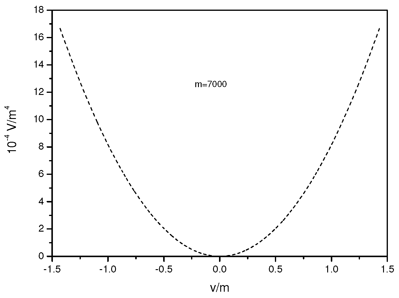
Since relation (12) holds, the terms proportional to $\frac{1}{L^2}$ cancel. Also, the minimum potential vanishes at $v=0$ and supersymmetry is preserved. Indeed, the behavior of (30) for small v we get:

$$V\simeq m_1^2{v}^2+O(v^3).$$

(31)

In figure 1, the plot of the effective potential for the upper perturbative limit $mL=1$ is shown. The other numerical values are chosen to be: $m_1=$200, $m=$7000, $g_1=$0.001, $g=$0.09, $\mu =$7000.

3. Addition of Explicit Supersymmetry Breaking Terms

At this point, we add in Lagrangian (9) various hard supersymmetry breaking terms of the form $g_3{\chi }^2{\phi }_i^2$ and $g_2\overline{\mathsf{\Psi }}\mathsf{\Psi }\chi$, where $g_3$ and $g_2$ are dimensionless couplings (and recall $\chi =v+{\phi }_{u_1}/\sqrt{2}$). These terms, being non holomorphic and hard, explicitly break supersymmetry and also have moebiosity zero. The index ’i’ runs over all the twisted scalar fields.

As previously referred to, the addition of such terms re-introduce quadratic divergences in the theory, namely,

$$\Delta m_{scalar}=\frac{1}{8{\pi }^2}(l_s-l_f^2){\Lambda }_{UV}^2,$$

(32)

with ${\Lambda }_{UV}^2$ a relevant upper cut-off of the theory and $l_s$, $l_f$ boson and fermion couplings.

Since $\chi$ develops a vacuum expectation value, the fields coupled to it will have an additional mass of the form $g_3{v}^2$ for bosons and $g_{2}v$ for fermions. Various combinations of the allowed terms can be added. However, the interesting features are only triggered by some of these. In the following, we shall give a detailed description of all the terms.

As it was previously referred to, for specific values of the parameters appearing in these terms, the result is a theory in which supersymmetry is unbroken when the length of the compact dimension is large, and as the radius decreases supersymmetry spontaneously breaks after a critical length. Thus, supersymmetry is only broken for small lengths. In the following, the cases for which this happens are described in detail.

3.1. A term of the form $g_3{\chi }^2{\phi }_{t_1}^2$

An interaction among a twisted boson and an untwisted boson is added, which acquires vacuum expectation value, namely $-g_3{\chi }^2{\phi }_{t_1}^2$. Since $\chi =v+{\phi }_{u_1}/\sqrt{2}$, the twisted boson ${\phi }_{t_1}$ will have additional contribution to it’s tree order mass. The masses now read,

$$\begin{array}{ccc}\hfill m_{b_1}^2& =& m_1^2+3g_1{m}_{1}v+3g_1^2{v}^2/2\hfill \\ \hfill m_{b_2}^2& =& m_1^2+g_1{m}_{1}v+g_1^2{v}^2/2\hfill \\ \hfill m_{t_1}^2& =& m^2+4gmv+4g^2{v}^2+g^2{m}_{1}v/\sqrt{2}+g^2{g}_1{v}^2/4+g_3{v}^2\hfill \\ \hfill m_{t_2}^2& =& m^2+4gmv-g^2{m}_{1}v/\sqrt{2}-g^2{g}_1{v}^2/4\hfill \\ \hfill m_{f_1}& =& m_1+g_{1}v,m_{f_2}=m+2gv.\hfill \end{array}$$

(33)

As expected $m_{t_1}^2+m_{t_2}^2-2m_{f_2}^2\ne 0$, since supersymmetry is hardly broken.

An interesting phenomenon occurs for this term and for a class of other terms. In detail, when the length of the compact dimension is small supersymmetry is broken, and is restored when the radius increases above a critical length $L_c$.

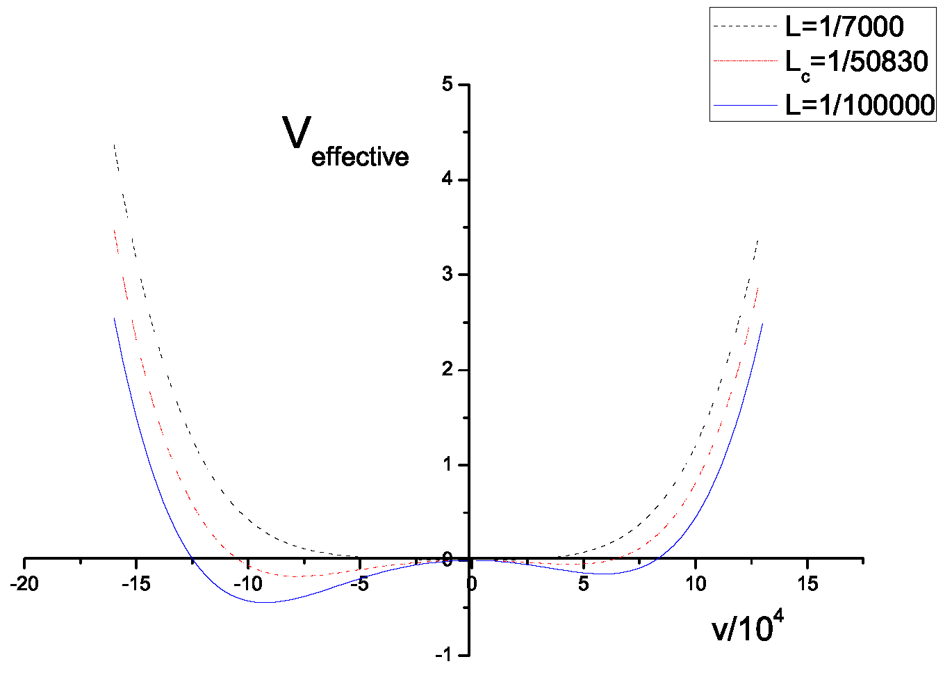
As can be seen in the next section, the behavior resembles the inverse symmetry breaking of continuous symmetries at finite temperature. A mentioned during the introduction, we call this “inverse supersymmetry breaking" for brevity. Inverse supersymmetry breaking can happen when $g_3$ is of the order of $\frac{m_1}{m}$ or for smaller values; that is $g_3\le \frac{m_1}{m}$ when only the term $g_3{\chi }^2{\phi }_{t_1}^2$ appears in the Lagrangian. This whole phenomenon is overviewed in figure 2. We use the following numerical values: $m_1=$200, $m=$7000, $g_1=$0.001, $g=$0.09, $\mu =$7000 and $g_3=0.05$.

As can be seen in figure 2, the phenomenon looks like a second order phase transition with the length of the compact dimension playing the role of the temperature. No barrier appears between the vacua at $v=0$ and at $v\ne 0$. The study was limited to perturbation theory preserving values of L. As it can be seen, for large L ($L=1/7000$) supersymmetry is unbroken and it starts to break at $L_c=1/50830$. As the length decreases, the breaking is all the more profound. It is also important to note that the two non- supersymmetric vacua are not equivalent. We tried to examine how $L_c$ changes under a change of $g_3$. In

Table 1. $g_3$ and the corresponding $L_c$ values, case $g_3{\chi }^2{\phi }_{t_1}^2$

${\mathit{g}}_3$	${\mathit{L}}_{\mathit{c}}^{-1}$
0.1	32319
0.07	41352
0.05	50839
0.03	67994
0.01	121950
0.007	145900
0.005	173083
0.003	223990
0.001	388990
0.0005	557000
0.0001	1232000
0.00005	1740000
0.00001	3942000

we present the values of $g_3$ and the corresponding values of $L_c$, and in

Table 2. Plot of the $L_c-g_3$ (left) and fit with a continuous curve (right), case $g_3{\chi }^2{\phi }_{t_1}^2$

we present the $L_c-g_3$ and the fit of the curve with a continuous function. The dots are the values that appear in Table 1, while the continuous line corresponds to the function $0.0000914\sqrt{x}$. Thus, the dependence of $g_3$ as a function of $L_c$ is roughly,

$$L_c^{-1}\sim 0.0000914\sqrt{g_3}.$$

(34)

Before ending this section, contour plots of the effective potential are presented as a function of $g_3$ and the classical values v. In

Table 3. Contour plots of the effective potential as a function of $g_3$ and $L_c$, case $g_3{\chi }^2{\phi }_{t_1}^2$

the $g_3-L_c$ behavior can be seen clearer. It is noticeable that as the colors become lighter, the values are larger. Finally, a term of the form $g_3{\chi }^2{\phi }_{t_2}^2$, an interaction between the other twisted scalar and of the untwisted scalar, gives similar results with the case we just studied. Even the fitting curve of the $L_c-g_3$ behavior is the same. We give in

Table 4. $g_3$ and the corresponding $L_c$ values for the $g_3{\chi }^2{\phi }_{t_2}^2$ case

${\mathit{g}}_3$	${\mathit{L}}_{\mathit{c}}^{-1}$
0.1	32290
0.07	41320
0.01	121551
0.0001	1238950
0.00001	3922000

some specific values in order to compare with Table 1

3.2. Combination of the terms $g_3{\chi }^2{\phi }_{t_1}^2$ and $g_3{\chi }^2{\phi }_{t_2}^2$

In the Lagrangian (6), we now add a combination of the terms $g_3{\chi }^2{\phi }_{t_1}^2$ and $g_3{\chi }^2{\phi }_{t_2}^2$. These terms describe interactions between the untwisted scalar and the two twisted scalar fields, respectively. Thus, the tree order masses of the twisted scalar fields are modified to:

$$\begin{array}{ccc}\hfill m_{t_1}^2& =& m^2+4gmv+4g^2{v}^2+g^2{m}_{1}v/\sqrt{2}+g^2{g}_1{v}^2/4+g_3{v}^2\hfill \\ \hfill m_{t_2}^2& =& m^2+4gmv-g^2{m}_{1}v/\sqrt{2}-g^2{g}_1{v}^2/4+g_3{v}^2\hfill \end{array}$$

(35)

and as before $m_{t_1}^2+m_{t_2}^2-2m_{f_2}^2\ne 0$. Now, as in the case where a single interaction term between the untwisted and twisted scalar, the conditions that must hold in order for inverse supersymmetry breaking to occur, are $g_3\le \frac{m_1}{m}$. What happens again then is described by Figure 2. In

Table 5. $g_3$ and the corresponding $L_c$ values, case $g_3{\chi }^2{\phi }_{t_1}^2$, $g_3{\chi }^2{\phi }_{t_2}^2$

${\mathit{g}}_3$	${\mathit{L}}_{\mathit{c}}^{-1}$
0.1	32300
0.07	41359
0.05	51009
0.03	68100
0.01	121900
0.005	173500
0.001	388990

we present the $g_3-L_c$ dependence and in

Table 6. Plot of the $L_c-g_3$ (right) and fit with a continuous curve (left), case $g_3{\chi }^2{\phi }_{t_1}^2$, $g_3{\chi }^2{\phi }_{t_2}^2$

we plot the $g_3-L_c$ and fit the curve with a continuous function,

As in (34), the fitted $L_c-g_3$ dependence is:

$$L_c^{-1}\sim 0.0000918\sqrt{g_3}.$$

(36)

This behavior is almost the same in the two cases, and motivates us to think that there is some kind of universality in the $L_c-g_3$ behavior. This aspect could possibly be used against the argument that the inverse supersymmetry breaking is just a perturbation theory artifact, but this will be analyzed thoroughly in the conclusion. In summary, this case has many similarities with the previous, with one twisted scalar breaking term.

3.3. Combination of the terms $\frac{1}{2}{g}_2{\overline{\mathsf{\Psi }}}_u{\mathsf{\Psi }}_u\chi$ and $g_3{\chi }^2{\phi }_{t_1}^2$

We now add in the Lagrangian the terms $\frac{1}{2}{g}_2{\overline{\mathsf{\Psi }}}_u{\mathsf{\Psi }}_u\chi$ and $g_3{\chi }^2{\phi }_{t_1}^2$, which describe interaction between the twisted scalar field and the untwisted fermion and twisted scalar, respectively. In this case, the untwisted fermion and one twisted scalar acquire additional mass terms:

$$\begin{array}{ccc}\hfill m_{t_1}^2& =& m^2+4gmv+4g^2{v}^2+g^2{m}_{1}v/\sqrt{2}+g^2{g}_1{v}^2/4+g_3{v}^2\hfill \\ \hfill m_{f_1}& =& m_1+g_{1}v+g_{3}v\hfill \end{array}$$

(37)

As expected $m_{t_1}^2+m_{t_2}^2-2m_{f_2}^2\ne 0$, and also $m_{b_1}^2+m_{b_2}^2-2m_{f_1}^2\ne 0$ since supersymmetry is hardly broken.

The conditions that must hold in order for inverse supersymmetry breaking to occur are $g_3\le \frac{m_1}{m}$, as in the previous cases and in addition $g_2\ll g_3$. For this condition, the behavior of supersymmetry breaking is well described from Figure 2 and inverse supersymmetry breaking occurs.

Table 7. $g_3$ and the corresponding $L_c$ values for the case $\frac{1}{2}{g}_2{\overline{\mathsf{\Psi }}}_u{\mathsf{\Psi }}_u\chi$, $g_3{\chi }^2{\phi }_{t_1}^2$

${\mathit{g}}_3$	${\mathit{L}}_{\mathit{c}}^{-1}$
0.1	32178
0.07	41205
0.05	50742
0.03	62250
0.01	84200
0.005	170000
0.001	381570

shows the $g_3-L_c$ dependence and in

Table 8. Plot of the $L_c-g_3$ (right) and fit with a continuous curve (left), for the case $\frac{1}{2}{g}_2{\overline{\mathsf{\Psi }}}_u{\mathsf{\Psi }}_u\chi$, $g_3{\chi }^2{\phi }_{t_1}^2$

we plot the $g_3-L_c$ and fit the curve with a continuous function. We fix the coupling to $g_2=0.0001$.

The fitted $L_c-g_3$ dependence is:

$$L_c^{-1}\sim 0.0000944\sqrt{g_3}.$$

(38)

Compared with (36) and (34), the behavior is slightly different but to the sixth decimal. Thus, one could say that the $L_c-g_3$ dependence is more or less the same.

Table 9. Contour plots of the effective potential as a function of $g_3$ and $L_c$, for the case $\frac{1}{2}{g}_2{\overline{\mathsf{\Psi }}}_u{\mathsf{\Psi }}_u\chi$, $g_3{\chi }^2{\phi }_{t_1}^2$

shows the contour plots of the effective potential as a function of $g_2$ and of the classical value v. The value of $g_3=0.1$ is fixed. The first conclusion we can show is that inverse supersymmetry breaking occurs, and the value of $g_3$ is fixed in this case, and the second that the potential is not affected by the value of $g_2$.

We omit the case $\frac{1}{2}{g}_2{\overline{\mathsf{\Psi }}}_u{\mathsf{\Psi }}_u\chi$, $g_3{\chi }^2{\phi }_{t_2}^2$ because it is identical with the one being just studied.

3.4. Combination of the terms $\frac{1}{2}{g}_2{\overline{\mathsf{\Psi }}}_u{\mathsf{\Psi }}_u\chi$, $g_3{\chi }^2{\phi }_{t_1}^2$ and $g_3{\chi }^2{\phi }_{t_2}^2$

The final case for which inverse supersymmetry breaking occurs is when interactions of the untwisted scalar $\chi$ are added along with the two twisted scalars and with the untwisted fermion. Thus, we add in the Lagrangian (6) the terms $\frac{1}{2}{g}_2{\overline{\mathsf{\Psi }}}_u{\mathsf{\Psi }}_u\chi$, $g_3{\chi }^2{\phi }_{t_1}^2$ and $g_3{\chi }^2{\phi }_{t_2}^2$. Thus the two untwisted scalars and the untwisted fermion acquire additional contributions to their tree order mass, which are:

$$\begin{array}{ccc}\hfill m_{t_1}^2& =& m^2+4gmv+4g^2{v}^2+g^2{m}_{1}v/\sqrt{2}+g^2{g}_1{v}^2/4+g_3{v}^2\hfill \\ \hfill m_{t_2}^2& =& m^2+4gmv-g^2{m}_{1}v/\sqrt{2}-g^2{g}_1{v}^2/4+g_3{v}^2\hfill \\ \hfill m_{f_1}& =& m_1+g_{1}v+g_{2}v.\hfill \end{array}$$

(39)

As usual $m_{t_1}^2+m_{t_2}^2-2m_{f_2}^2\ne 0$ and $m_{b_1}^2+m_{b_2}^2-2m_{f_1}^2\ne 0$.

The conditions that must hold in order for inverse supersymmetry breaking to occur are as before, $g_3\le \frac{m_1}{m}$, as in the previous cases and in addition $g_2\ll g_3$. For this condition the behavior of supersymmetry breaking is again well described from Figure 2 and inverse supersymmetry breaking occurs. In

Table 10. $g_3$ and the corresponding $L_c$ values for the case $\frac{1}{2}{g}_2{\overline{\mathsf{\Psi }}}_u{\mathsf{\Psi }}_u\chi$, $g_3{\chi }^2{\phi }_{t_1}^2$, $g_3{\chi }^2{\phi }_{t_2}^2$

${\mathit{g}}_3$	${\mathit{L}}_{\mathit{c}}^{-1}$
0.1	32350
0.07	41900
0.05	50900
0.03	67990
0.01	121500
0.005	172000
0.001	300000

the $g_3-L_c$ dependence is shown and in

Table 11. Plot of the $L_c-g_3$ (right) and fit with a continuous curve (left), for the case $\frac{1}{2}{g}_2{\overline{\mathsf{\Psi }}}_u{\mathsf{\Psi }}_u\chi$, $g_3{\chi }^2{\phi }_{t_1}^2$, $g_3{\chi }^2{\phi }_{t_2}^2$

the $g_3-L_c$ is plotted and the curve fit with a continuous function. The coupling is fixed to $g_2=0.0001$.

The fitted $L_c-g_3$ dependence is:

$$L_c^{-1}\sim 0.0000916\sqrt{g_3}.$$

(40)

Compare with (36) and (34) and (38). The behavior that relation (40) describes is the same with that of (36) and (34). This cannot be accidental. We shall discuss this in the next subsection.

3.5. Discussion

Previously, we showed for which combinations of terms inverse supersymmetry breaking occurs. In this section, we show which terms do not give inverse supersymmetry breaking. These are:

• Addition of fermion interactions with the untwisted scalar of the form

  *

  $\frac{1}{2}{g}_2{\overline{\mathsf{\Psi }}}_u{\mathsf{\Psi }}_u\chi$

  *

  $\frac{1}{2}{g}_2{\overline{\mathsf{\Psi }}}_t{\mathsf{\Psi }}_t\chi$

  *

  $\frac{1}{2}{g}_2{\overline{\mathsf{\Psi }}}_u{\mathsf{\Psi }}_u\chi$ and $\frac{1}{2}{g}_2{\overline{\mathsf{\Psi }}}_t{\mathsf{\Psi }}_t\chi$

• Addition of interactions of twisted fermions with twisted scalars of the form

  *

  $\frac{1}{2}{g}_2{\overline{\mathsf{\Psi }}}_t{\mathsf{\Psi }}_t\chi$, $g_3{\chi }^2{\phi }_{t_1}^2$

  *

  $\frac{1}{2}{g}_2{\overline{\mathsf{\Psi }}}_t{\mathsf{\Psi }}_t\chi$, $g_3{\chi }^2{\phi }_{t_2}^2$

  *

  $\frac{1}{2}{g}_2{\overline{\mathsf{\Psi }}}_t{\mathsf{\Psi }}_t\chi$, $g_3{\chi }^2{\phi }_{t_1}^2$, $g_3{\chi }^2{\phi }_{t_2}^2$

In principle any interaction involving untwisted scalar and twisted fermion interactions, $\frac{1}{2}{g}_2{\overline{\mathsf{\Psi }}}_t{\mathsf{\Psi }}_t\chi$, does not trigger inverse supersymmetry breaking. This holds for any combination of terms we add along with the above. Also, any fermion-untwisted scalar interaction appearing itself does not give inverse supersymmetry breaking.

As it was previously shown, in all the cases when inverse supersymmetry breaking occurs, it is followed by a kind of universal behavior. This is focused mainly in the $L_c-g_3$ dependence. This universality (if this term can be used) is expressed by:

$$L_c^{-1}\sim 0.000091\sqrt{g_3}.$$

(41)

This is an interesting feature and it can be claimed that it cannot be accidental. Thus, this could stand against the argument that inverse supersymmetry breaking is an artifact of perturbation theory. Also, the theory remains, at some level, supersymmetric, and we do not expect dramatic changes when higher loop calculations are incorporated.

4. Inverse Symmetry Breaking and Symmetry non-Restoration at Finite Temperature

In this section we review similar phenomena to ones that were previously described. The difference is that in this section symmetries are studied at finite temperature and the symmetry that is involved is not supersymmetry, but a continuous global $O(N_1)\times O(N_2)$ or a discrete $Z_2\times Z_2$. As it will be shown, symmetry non-restoration and inverse symmetry breaking phenomena can occur, when terms similar to $\frac{1}{2}{g}_2\overline{{\psi }_t}{\psi }_t\chi$, $g_3{\chi }^2{\phi }_{t_1}^2$ appear in the Lagrangian.

Symmetry non-restoration means that a symmetry broken at $T=0$ never gets restored at high temperatures. Inverse symmetry breaking means that an unbroken symmetry at $T=0$ may be spontaneously broken at high temperature.

These phenomena occur in field theories when cross interactions are included among the scalar fields similar to the bosonic hard supersymmetry breaking term $g_3{\chi }^2{\phi }_{u_2}^2$ or other crossed terms that were used. Similar to this term, scalar interactions and also Yukawa terms like the ones of the previous sections, are frequently used in the theory of reheating after inflation. In actual fact, these similarities motivated us to use such terms in order to show their impact on supersymmetry breaking.

The inverse symmetry breaking phenomenon is briefly reviewed here. The setup is a theory with real scalar fields ${\varphi }_1$ and ${\varphi }_2$ described by the $O(N_1)\times O(N_2)$ globally symmetric Lagrangian,

$$\begin{array}{c}L=\frac{1}{2}{\partial }_{\mu }{\varphi }_1{\partial }_{\mu }{\varphi }_1+\frac{1}{2}{\partial }_{\mu }{\varphi }_2{\partial }_{\mu }{\varphi }_2+\frac{1}{2}{m}_1^2{\varphi }_1^2+\frac{1}{2}{m}_2^2{\varphi }_2^2+\frac{1}{4!}{\lambda }_1{\varphi }_1^4+\frac{1}{4!}{\lambda }_1{\varphi }_2^4+\frac{1}{4!}\lambda {\varphi }_1^2{\varphi }_2^4,\hfill \end{array}$$

(42)

where ${\varphi }_1$ and ${\varphi }_2$ be real scalars with $N_1$ and $N_2$ components. In the above Lagrangian one of the global $O(N_i)$ symmetries may break at high temperature if the $\lambda$ coupling takes negative values. Thus, one of the two scalar fields ${\varphi }_1$ or ${\varphi }_2$ may acquire a non-zero vacuum expectation value. Therefore, at high temperature and for certain values of the parameters, the initial $O(N_1)\times O(N_2)$ is broken to $O(N_1)$. This so-called inverse symmetry breaking was first pointed out by Weinberg [26] and has been extensively studied by many authors [36,37,38,39,40,41].

Symmetry non-restoration was used in [40] to solve the monopole problem in the $SU(5)$ GUT. As was proposed in [40], the symmetric phase of $SU(5)$ was never realized, no matter how high the temperature became. In that paper, the interaction term $\alpha |{\chi }_{45}{|}^2\left|H_{24}\right|$ appearing in the scalar Kibble-Higgs sector is responsible for the non-restoration of the $SU(5)$ symmetry. Actually, the scalar interaction of $H_{24}$ and ${\chi }_{45}$ gives negative contributions to the thermal masses and one of those become negative. When this takes place, the corresponding Higgs field acquires a vacuum expectation value for high temperatures and the symmetry is never restored. This phenomenon occurs for certain values of the parameters (see [37,40]).

The intuitive approach to all phenomena at finite temperature is based on the fact that symmetries broken at low temperatures may become restored at high temperature (in the same class belong finite volume theories). Counter-intuitive phenomena occur in field theories with rich scalar sector. Especially, if the multi-scalar sectors interact weakly with negative couplings, then as we have seen, the phenomena like inverse symmetry breaking or symmetry non-restoration occur. This happens at high temperature and refers to the spontaneous breaking of a symmetry at high temperature. Usually the symmetry is a global $O(N_1)\times O(N_2)$ or for the case of symmetry non-restoration continuous, like $SU(5)$.

Although inverse symmetry breaking is counter-intuitive, nature has provided us with cases where systems are more symmetric at low temperatures than at high temperature. The Rochelle salt and physics of liquid crystals are two examples.

Before closing this section, it is essential to note that similar terms to those we used appear in the reheating after inflation process. The Lagrangian governing this process is,

$$\begin{array}{c}L=\frac{1}{2}{({\partial }_{\mu }\phi )}^2-\frac{m_{\phi }}{2}{\phi }^2+\frac{1}{2}{({\partial }_{\mu }\chi )}^2-\frac{m_{\chi }}{2}{\chi }^2+\overline{\psi }(i{\gamma }^{\mu }{\partial }_{\mu }-m_{\psi })\psi -\lambda \phi \overline{\psi }\psi -\frac{1}{2}{g}^2{\phi }^2{\chi }^2.\hfill \end{array}$$

(43)

The role of the inflaton field is played by the scalar field $\phi$. The inflaton field decays to the particles $\psi$ and $\chi$ due to the interaction terms $\lambda \phi \overline{\psi }\psi$ and $\frac{1}{2}{g}^2{\phi }^2{\chi }^2$. It is noticeable that similar terms are used in order to break supersymmetry hard and all the effects that are shown in the previous section are due to these interaction terms. Also, in order for reheating to take place, the condition $m_{\phi }\gg m_{\psi },m_{\chi }$ must hold (it is noticeable that similar conditions hold in the supersymmetric model that are previously studied). There, $m_1$ was the tree order mass of the untwisted scalar field and m the tree order mass of the twisted scalar. One of the conditions used is that the untwisted sector mass is larger than the twisted sector one, namely $m_1\gg m$. Also the untwisted fermion has mass m [8].

5. Conclusions

In this paper, a simple supersymmetric model was studied in $S^1\times R^3$ spacetime topology. The way that topology affects the boundary conditions was reviewed. In addition, it was depicted that supersymmetry breaks spontaneously at finite volume, and how this can be avoided in terms of the boundary conditions that the fields obey. The effective potential was calculated and it was shown that with the appropriate boundary conditions supersymmetry remains intact.

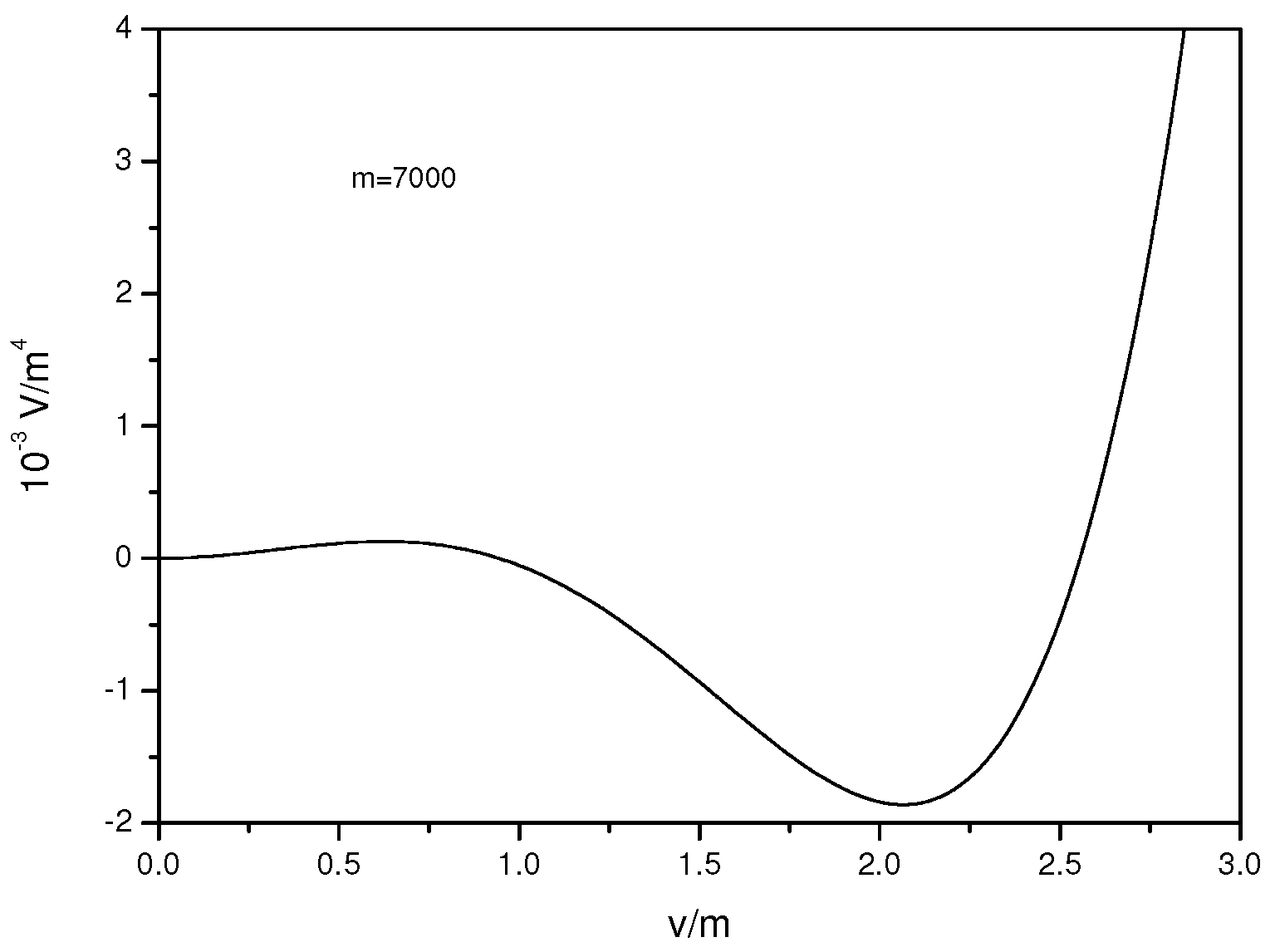
In addition, interaction terms among scalars and fermions were introduced in the Lagrangian. These terms cause hard supersymmetry breaking, when the topology is $R^4$ topology. This appears in the plot of the effective potential for the case where the compact radius is infinite (see Figure 3).

It seems that in $S^1\times R^3$ something different occurs. It could be possibly assumed that supersymmetry remains broken when the compact radius remains finite. However, this does not take place when one loop finite volume corrections are taken into account. As it was shown, the addition of hard supersymmetry breaking interactions among the scalars of the untwisted sector that develop a vacuum expectation value and the twisted scalars or the twisted fermions, results in a very peculiar phenomenon. In particular, when certain conditions hold, which are similar to the aforementioned, supersymmetry is broken for small lengths, and as the radius increases supersymmetry becomes restored after a critical length. This was referred to as “inverse supersymmetry breaking" for brevity. This conceptually resembles second order phase transitions. In particular, we presented all the combinations of terms for which inverse supersymmetry breaking occurs. The result was that it works only for twisted boson and untwisted fermions combinations (but never for fermion interactions alone).

In addition, it was found that there is a universality in the $L_c-g_3$ behavior. Specifically, it seems that, with a sixth-decimal accuracy, the $L_c-g_3$ dependence can be described by:

$$L_c^{-1}\sim 0.00009\sqrt{g_3}.$$

(44)

This holds for all the cases that inverse supersymmetry breaking can occur. This fact led to our assumption that inverse supersymmetry breaking cannot be a consequence of coupling interplay and maybe one loop physics artifact. The last can be augmented by the fact that the theory remains at some level supersymmetric and the two loop results will not change dramatically the one loop results.

We found conceptual similarities between inverse supersymmetry breaking and inverse symmetry breaking phenomena at finite temperature, which occur in field theories with a rich scalar sector. In that case a symmetry unbroken at low temperatures may break at high temperature. In our case, at small lengths supersymmetry breaks, while it remains unbroken at large radius values. The terms in the Lagrangian that trigger inverse symmetry breaking are the same that trigger inverse supersymmetry breaking. Also, these terms appear in the theory of reheating and in the thermal inflation.

To end this paper, the physical significance of “inverse supersymmetry breaking" can be shown. This phenomenon is not so appealing to a four-dimensional theory. What would be expected is that supersymmetry should be unbroken for small values of the radius of the compact dimension and should break dynamically at large radius. However, we discuss that what actually happens is the converse: for large values of the radius supersymmetry is unbroken and dynamically breaks for small values of the radius. This would be interesting for a five-dimensional model. Imagine a theory where supersymmetry is unbroken for a large radius of the compact dimension and breaks dynamically for small values of the compact dimension. It is an intriguing task to find what this mechanism, which has something to do with coupling interplay between interactions, has to say for the radius stabilization mechanism and the supersymmetry breaking mechanisms of extra dimensional models.

References

- Avis, S. J.; Isham, C. J. Generalized spin structures on four dimensional space-times. Commun. Mathe. Phys. 1980, 72, 103–118. [Google Scholar] [CrossRef]
- Ford, L. H. Vacuum polarization in a nonsimply connected Spacetime. Phys. Rev. D 1980, 21, 933–948. [Google Scholar] [CrossRef]
- Goncharov, Yu. P.; Bytsenko, A. A. Topological violation of supersymmetry. Phys. Lett. B 1985, 163, 155–160. [Google Scholar] [CrossRef]
- Toms, D. J. The Casimir Effect And Topological Mass. Phys. Rev. D 1980, 21, 928–932. [Google Scholar] [CrossRef]
- Toms, D. J. Symmetry Breaking And Mass Generation By Space-Time Topology. Phys. Rev. D 1980, 21, 2805–2817. [Google Scholar] [CrossRef]
- Toms, D. J. Interacting Twisted And Untwisted Scalar Fields In A Nonsimply Connected Space-Time. Ann. Phys. 1980, 129, 334–357. [Google Scholar] [CrossRef]
- Linde, A. D. Particle Physics and Inflationary Cosmology; CRC Press: Florida, USA, 1990. [Google Scholar]
- Kofman, L.; Linde, A.; Starobinsky, A. A. Reheating after Inflation. Phys. Rev. Lett. 1994, 73, 3195–3198. [Google Scholar] [CrossRef] [PubMed]
- Starobinsky, A. A. A new type of isotropic cosmological models without singularity. Phys. Lett. B 1980, 91, 99–102. [Google Scholar] [CrossRef]
- Vilenkin, A. Birth of inflationary universes. Phys. Lett. B 1983, 27, 2848–2855. [Google Scholar] [CrossRef]
- Guth, A. H.; Tye, S. H. H. Phase Transitions and Magnetic Monopole Production in the Very Early Universe. Phys. Rev. Lett. 1980, 44, 631–635. [Google Scholar] [CrossRef]
- Buchbinder, I. L.; Odintsov, S. D. Effective Action In Multidimensional (Super)Gravities And Spontaneous Compactification. (Quantum Aspects Of Kaluza-Klein Theories). Fortshrt. Phys. 1989, 37, 225–259. [Google Scholar] [CrossRef]
- Buchbinder, I. L.; Odintsov, S. D. Effective potential in A curved Space-Time. J. Sov. Phys. 1984, 27, 554–558. [Google Scholar] [CrossRef]
- Buchbinder, I. L.; Odintsov, S. D. One loop renormalization of the Yang-Mills field theory in A Curved Space-Time. J. Sov. Phys. 1983, 26, 359–361. [Google Scholar] [CrossRef]
- Odintsov, S. D. Casimir Effect In Multidimensional Quantum Supergravities And Supersymmetry Breaking. Mod. Phys. Lett. A 1988, 3, 1391–1399. [Google Scholar] [CrossRef]
- Odintsov, S. D. Two loop effective potential in quantum field theory in curved space-time. Phys. Lett. B 1993, 306, 233–236. [Google Scholar] [CrossRef]
- Elizalde, E.; Odintsov, S. D.; Romeo, A. Zeta regularization of the O(N) nonlinear sigma model in D-dimensions. J. Math. Phys. 1996, 37, 1128–1147. [Google Scholar] [CrossRef]
- Elizalde, E.; Odintsov, S. D.; Romeo, A. Effective potential for a covariantly constant gauge field in curved space-time. Phys. Rev. D 1996, 54, 4152–4159. [Google Scholar] [CrossRef]
- Elizalde, E.; Nojiri, S.; Odintsov, S. D.; Ogushi, S. Casimir effect in de Sitter and anti-de Sitter brane worlds. Phys. Rev. D 2003, 67, 063515. [Google Scholar] [CrossRef]
- Lavrov, P. M.; Odintsov, S. D. I. V. Tyutin Effective actions in quantum gravity theories. Sov. J. Nucl. Phys. 1987, 46, 932–936. [Google Scholar]
- Odintsov, S. D. Renormalization Group, Effective Action And Grand Unification Theories In Curved Space-Time. Fortsch. Phys. 1991, 39, 621–641. [Google Scholar] [CrossRef]
- Dowker, J. S.; Banach, R. Quantum Field Theory On Clifford-Klein Space-Times. The Effective Lagrangian And Vacuum Stress Energy Tensor. J. Phys. A: Math. Theor. 1978, 11, 2255–2284. [Google Scholar] [CrossRef]
- Dowker, J. S.; Banach, R. Automorphic Field Theory: Some Mathematical Issues. J. Phys. A: Math. Theor. 1979, 12, 2527–2543. [Google Scholar]
- Martin, S. P. Two-loop effective potential for a general renormalizable theory and softly broken supersymmetry. Phys. Rev. D 2002, 65, 116003. [Google Scholar] [CrossRef]
- Dolan, L.; Jackiw, R. Symmetry behavior at finite temperature. Phys. Rev. D 1974, 9, 3320–3341. [Google Scholar] [CrossRef]
- Weinberg, S. Gauge and global symmetries at high temperature. Phys. Rev. D 1974, 9, 3357–3378. [Google Scholar] [CrossRef]
- Elizalde, E. Ten physical applications of spectral zeta functions; Springer-Verlag: Berlin Heidelberg, Germany, 1995. [Google Scholar]
- Elizalde, E.; Odintsov, S. D.; Romeo, A.; Bytsenko, A. A.; Zerbini, S. Zeta regularization techniques and applications; World Scientific: Singapore, 1994. [Google Scholar]
- Kirsten, K. Spectral Functions in Mathematics and Physics; Chapman & Hall/CRC: Florida, USA, 2002. [Google Scholar]
- Oikonomou, V. K. Report of the Detailed Calculation of the Effective Potential in Spacetimes with S1 × Rd Topology and at Finite Temperature. Rev. Math. Phys. 2009, 21, 615–674. [Google Scholar] [CrossRef]
- Elizalde, E.; Kirsten, K. Topological symmetry breaking in selfinteracting theories on toroidal space-time. J. Math. Phys. 1994, 35, 1260–1273. [Google Scholar] [CrossRef]
- Odintsov, S. D. Compactification And Spontaneous Symmetry Breaking In The Lambda Phi4 Theory With Kaluza-Klein Background. J. Sov. Phys. 1988, 31, 695–699. [Google Scholar] [CrossRef]
- Elizalde, E; Odintsov, S. D.; Leseduarte, S. Chiral symmetry breaking in the Nambu-Jona-Lasinio model in curved space-time with nontrivial topology. Phys. Rev. D 1994, 49, 5551–5558. [Google Scholar] [CrossRef]
- Brevik, I; Milton, K; Nojiri, S; Odintsov, S. D. Quantum (in)stability of a brane world AdS(5) universe at nonzero temperature. Nucl. Phys. B 2001, 599, 305–318. [Google Scholar] [CrossRef]
- Kirsten, K. Casimir effect at finite temperature. J. Phys. A: Math. Theor. 1991, 24, 3281–3298. [Google Scholar] [CrossRef]
- Bimonte, G.; Lozano, G. On symmetry non-restoration at high temperature. Phys. Lett. B 1996, 366, 248–252. [Google Scholar] [CrossRef]
- Bimonte, G.; Lozano, G. Can symmetry non-restoration solve the monopole problem? Nucl. Phys. B 1996, 460, 155–166. [Google Scholar] [CrossRef]
- Pinto, M. B.; Ramos, R. O. A Nonperturbative study of inverse symmetry breaking at high temperatures. Phys. Rev. D 2000, 61, 125016. [Google Scholar] [CrossRef]
- Pinto, M. B.; Ramos, R. O.; Parreira, J. E. Phase transition patterns in relativistic and nonrelativistic multi-scalar-field models. Phys. Rev. D 2005, 71, 123519. [Google Scholar] [CrossRef]
- Dvali, G.; Melfo, A.; Senjanovic, G. Symmetry Nonrestoration at High Temperature and the Monopole Problem. Phys. Rev. Lett. 1995, 75, 4559–4562. [Google Scholar] [CrossRef] [PubMed]
- Pinto, M. B.; Ramos, R. O.; de Souza Cruz, F. F. Effective potential and thermodynamics for a coupled two-field Bose-gas model. Phys. Rev. A 2005, 74, 033618. [Google Scholar] [CrossRef]
Figure 1.
The supersymmetric effective potential
Figure 2.
Inverse Supersymmetry Breaking
Figure 3.
The continuum effective potential