Article

High-Resolution Hyperspectral Mineral Mapping: Case Studies in the Edwards Limestone, Texas, USA and Sulfide-Rich Quartz Veins from the Ladakh Batholith, Northern Pakistan

Department of Earth and Atmospheric Sciences, University of Houston, Houston, TX 77204, USA
*
Author to whom correspondence should be addressed.
Submission received: 7 September 2020 / Revised: 24 October 2020 / Accepted: 27 October 2020 / Published: 29 October 2020
(This article belongs to the Special Issue Remote Sensing-based Mineral Exploration)

Abstract

:
The study of hand samples is a significant aspect of geoscience. This work showcases a technique for relatively quick and inexpensive mineral characterization, applied to a Cretaceous limestone formation and for sulfide-rich quartz vein samples from Northern Pakistan. Spectral feature parameters are derived from mineral mixtures of known abundance and are used for mineral mapping. Additionally, three well-known classification techniques—Spectral Angle Mapper (SAM), Support Vector Machine (SVM), and Neural Network—are compared. Point counting results from petrographic thin sections are used for validation the limestone samples, and QEMSCAN mineral maps for the sulfide samples. For classifying the carbonates, the SVM classifier produced results that are closest to the training set—with 84.4% accuracy and a kappa coefficient of 0.8. For classifying sulfides, SAM produced mineral abundances that were closest to the validation data, possibly due to the low reflectance of sulfides throughout the short-wave infrared spectrum with some differences in the overall spectral shape.

1. Introduction

Applications of hyperspectral imaging (HSI) are gaining popularity in various fields such as agriculture [1,2], food quality monitoring [3,4], medical studies [5,6], forensics [7,8], geologic studies [9,10,11,12,13], and many others [14,15,16]. Recently, close-range HSI has been implemented as a non-invasive, high-resolution alternative to traditional methods of chemical characterization of materials of interest. Various classification algorithms have been applied to hyperspectral images to map endmember materials [17,18,19]. The same algorithms are applied to RADARSAT-2 polarimetric Synthetic Aperture Radar data for land cover mapping [20].
In geological applications, the resolution of laboratory-based HSI has been at the centimeter [21] to micrometer [22] scale. Recently, lenses with higher focal length have been used with short wave infrared (SWIR) cameras, which allow for pixels as small as 26 µm [23,24]. In geological applications, high-resolution imaging has the potential for increased accuracy of mineral abundance calculations. This can be significant for resource characterization because mineral distribution maps can be used for predictive modeling of the abundance of materials of interest [25,26,27].
Traditional techniques for fine-scale mineral mapping of rock chips can be costly. Techniques such as Quantitative Evaluation of Minerals by Scanning Electron Microscopy (QEMSCAN), Electron probe microanalyses (EPMA), and Mineral Liberation Analysis can be expensive, and thin section preparation can be time consuming (several weeks in most cases). Thin section point counting can be prone to user error [28], although recently automated techniques have been suggested for automating the estimation of porosity and mineral texture in thin section photomicrographs [29]; however, this method does not discriminate mineralogy.
Previously, high-resolution mineralogical mapping using hyperspectral imaging was validated using Scanning Electron Microscopy (SEM)-based Mineral Liberation Analyzer (MLA) [30,31]. This study presents two case studies, including sample suites that are compositional endmembers: diagenetically altered carbonates and sulfide mineral-rich quartz veins.

2. Materials and Methods

2.1. Sample Origins and Descriptions

Samples of the Edwards Limestone in the Lake Georgetown Spillway area were collected in 2014 (Figure 1). Pre-measured mineral mixtures were evaluated, similarly to Zaini et al. [32], but with the addition of silica to better estimate mineral abundances in the outcrop. A description of minerals used for reference spectra, field samples, thin section photomicrographs, and the geologic context of the Edwards Formation and sampling locations can be found within [33]. Samples were point counted using polished thin sections: 300–350 points were counted within a defined grid in the stained half of each thin section.
Quartz vein intrusions into diorite within the Ladakh batholith from the Astore area, located in Northern Pakistan, consisting of chalcopyrite and galena-rich quartz veins, were collected from the Astore Valley in Northern Pakistan (Figure 2). In previous studies, these samples were analyzed using QEMSCAN at Colorado School of Mines, and the results suggest that gold mineralization is associated with base metal sulfides, specifically chalcopyrite and galena [34,35].
Various mineral types have distinguishing features in the SWIR spectral region, including phyllosilicates, carbonates, hydroxides, sulfates, and others [36,37,38,39]. Carbonate minerals have a robust spectral feature in the within the wavelength ranges of 2530–2541 nm and 2333–2340 nm and 2503–2520 nm and 2312–2323 nm, respectively [32,40,41,42,43,44,45]. On the other hand, tectosilicates, such as quartz and feldspar, do not have distinctive features in SWIR but do in the thermal infrared spectral range [42,46]. Sulfide minerals such as pyrite and chalcopyrite are opaque and do not have any distinguishing features in SWIR [47,48]; however, some studies have used differences in spectral shape to distinguish them [21].

2.2. Mineral Mixture Preparation and Evaluation

Calcite, dolomite, and chert mixtures were prepared from relatively pure minerals, sieved to a grain size fraction of 75–150 µm, and mixed with the weight proportions in Table 1. Their spectral curves were measured using an Analytical Spectral Device (ASD) Fieldspec Pro spectroradiometer (Fieldspec Pro FR, Malvern Panalytical, Malvern, UK) under artificial illumination. Spectral parameters were calculated using Dispec (IDL DISPEC 3.6, ITC, Enschede, Netherlands), an IDL plugin for ENVI [49]. Mineral mixtures and rock chips were also scanned using the OLES 22.5 wide-angle (24° FOV) lens and a pixel size of 0.4 mm.

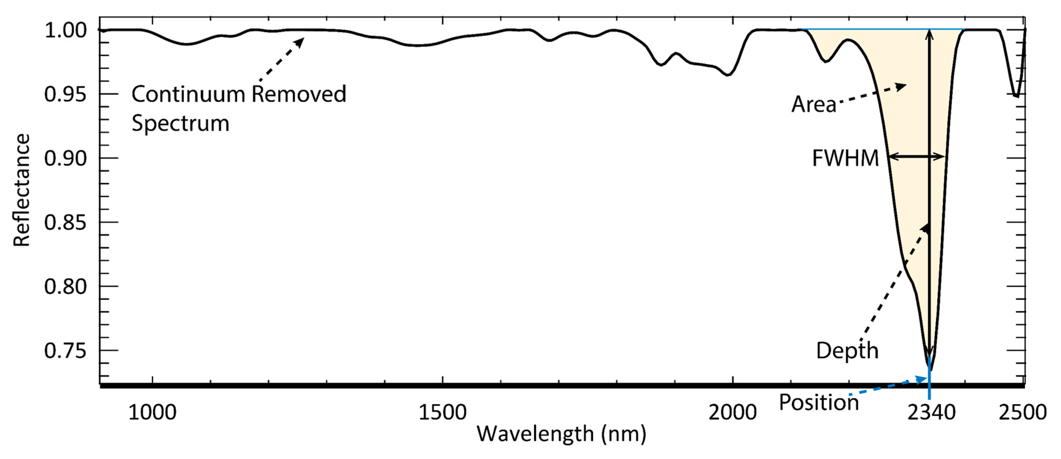
2.3. Hyperspectral Data Acquisition, Processing, and Classification

Laboratory-based HSI was conducted using a Specim SWIR camera (Spectral Camera SWIR, Specim, Oulu, Finland), operating within the 909–2503 nm spectral range, with 14-bit radiometric resolution. For high-resolution scanning, Specim’s OLES Macro lens (OLES Macro, Specim, Oulu, Finland) was used, which provides 1:1 imaging with a 7.5° field of view (FOV). Samples were placed on a scanning stage 0.10 m from the camera lens, with a spatial resolution of 32 µm. Three 50-Watt quartz halogen light bulbs were used for illumination. Samples were moved at a constant speed in the along-track direction. A frame rate of 100 Hz was selected to produce square pixels.
For hyperspectral data, pre-processing steps included dark frame subtraction, empirical line calibration [50], correcting image artifacts that occur in the along-track direction [51], and Savitzky–Golay spectral smoothing using a second order polynomial and a filter width of four bands [52,53]. All image processing and analysis techniques were implemented using ENVI software (Version 5.5, Harris Geospatial, Boulder, CO, USA) and Matlab 2018a (Mathworks, Inc, Natick, MA, USA).
Numerous mineral groups have distinct absorption features in the SWIR wavelengths that can be used as an indicator of mineralogy. For example, calcite has an absorption located at approximately 2330–2340 nm; this feature can be used to distinguish calcite from dolomite, which has an absorption feature of similar magnitude but located at shorter wavelengths, approximately 2315–2320 nm [44]. The wavelength location of an absorption feature minimum can be used to distinguish carbonate minerals, as well as many others [37,54] (Figure 3). The magnitude of absorption depth has been correlated with a higher concentration of the mineral in question [10,55] and can increase with larger grain size [56]. For carbonate samples, hyperspectral images of relatively pure mineral mixtures (Figure 4) were used to set thresholds for absorption minimum location. Minimum wavelength was mapped using the Hyperspectral Python program (HypPy, University of Twente, Enschede, Netherlands) [57].
Three classification techniques were compared. Spectral Angle Mapper (SAM) classifies image pixels by treating each pixel and reference (endmember) spectrum as a vector in a space with dimensionality equal to the number of image bands [58]. The angle between each pixel vector and the reference vector is used to produce a classification image based on a user-defined threshold. This technique is relatively simple and can use training data from various sources. Computation time is typically short.
Support Vector Machine (SVM) is a technique derived from statistical learning theory, which separates classes with a decision surface that maximizes the boundary between classes [59,60,61]. Support vectors or the data points closest to the decision surface, are elements of the training set. Previous studies report that this technique yields reliable results with noisy data, although training time can be long depending on the amount of training data that is input [62]. A drawback in the SVM algorithm is its reported poor performance in classifying hyperspectral data with a model learned from independent training data [63], potentially due to differences in illumination [64]. A kernel function is used to assign weights of nearby points for classification. For the present study, the radial basis function was used. A probability threshold of 0.5 was set for these examples, so that at least 50% of bands must match the class to be assigned.
Implementation of the Neural Network classification in ENVI is a layered feed-forward classification technique with error backpropagation for supervised learning. The weights in the node are adjusted to minimize the difference between the output node activation and input. A training threshold contribution is set to determine the size of the contribution of the internal weight and is used to adjust the changes to the internal weight [65]. A larger weight leads to poor generalizations but more accurate classification. For this work, a training threshold contribution of 0.95 was set after testing several other values. Non-linear neural network classification requires at least one hidden layer, and the number of hidden layers needed depends on the complexity of the decision surface for the classification [59]. The minimum output activation threshold was set to 0.5, such that if the activation value of a pixel for any given class is less than 0.5, it remains unclassified.

3. Results

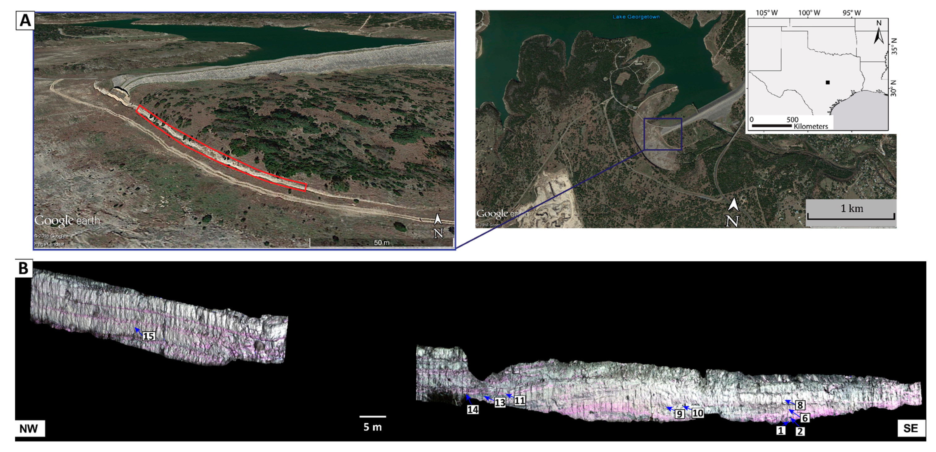
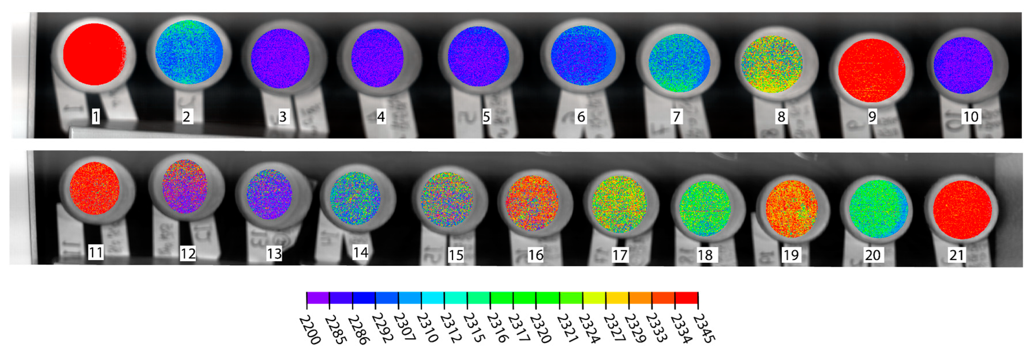
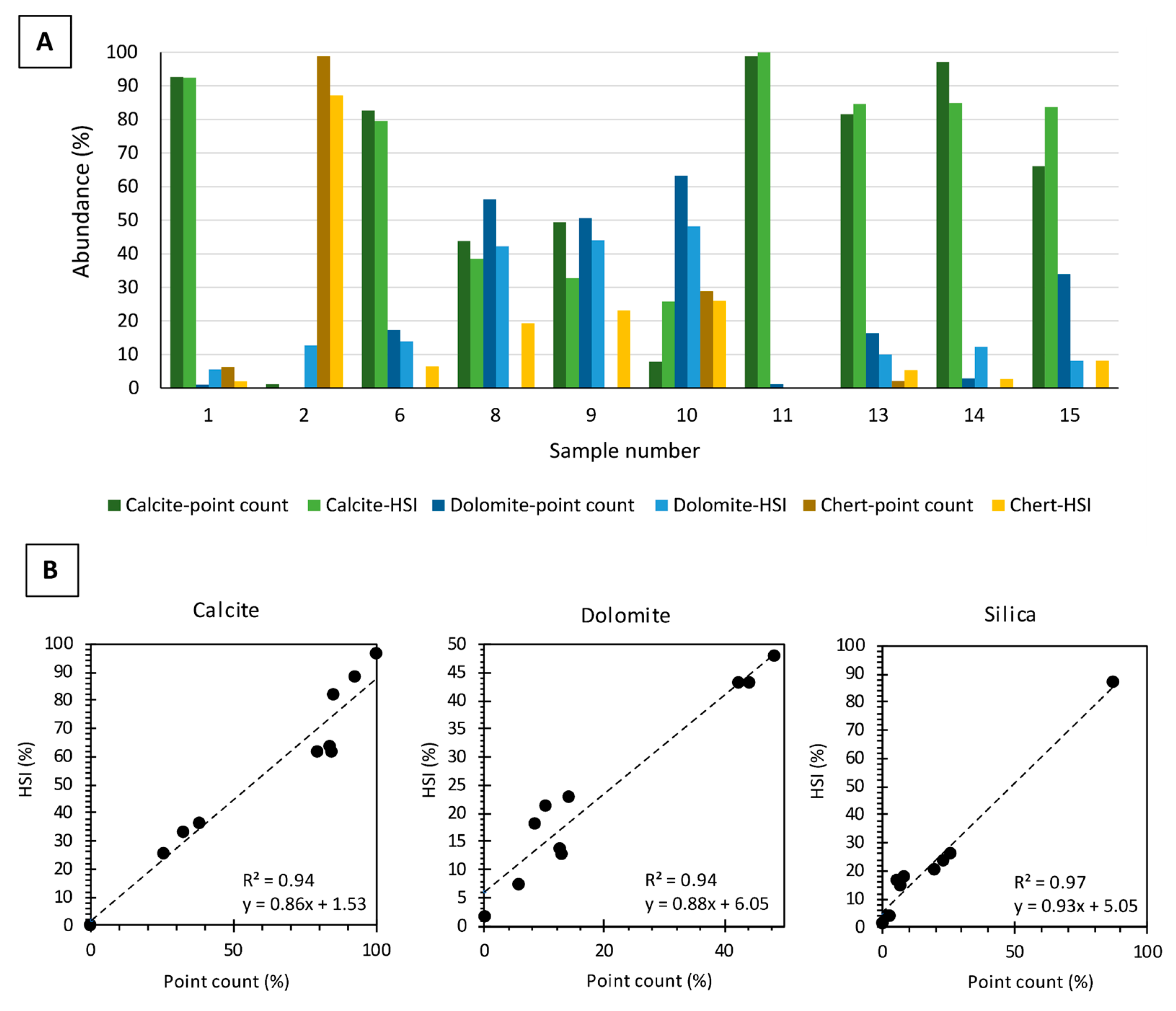
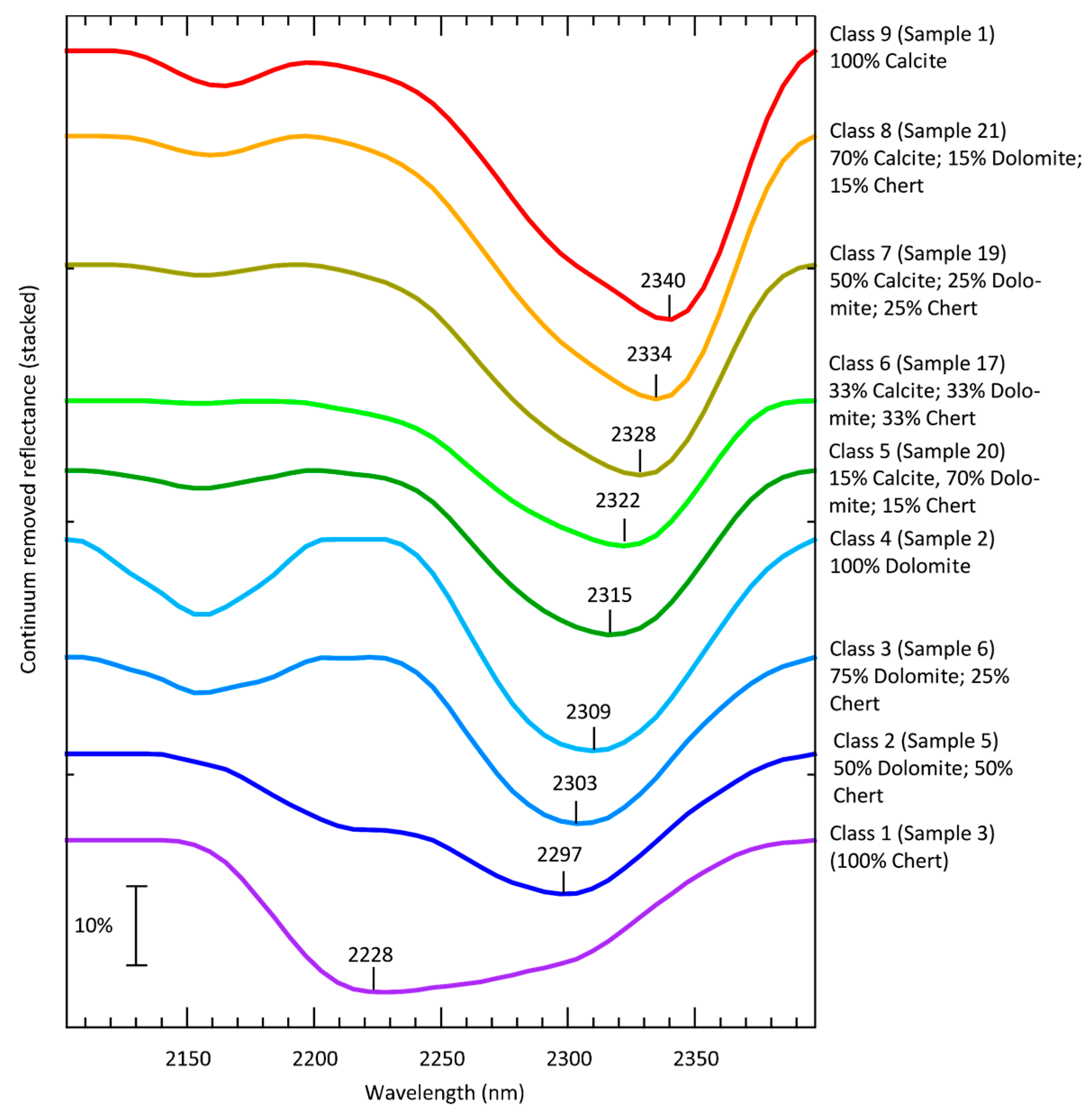
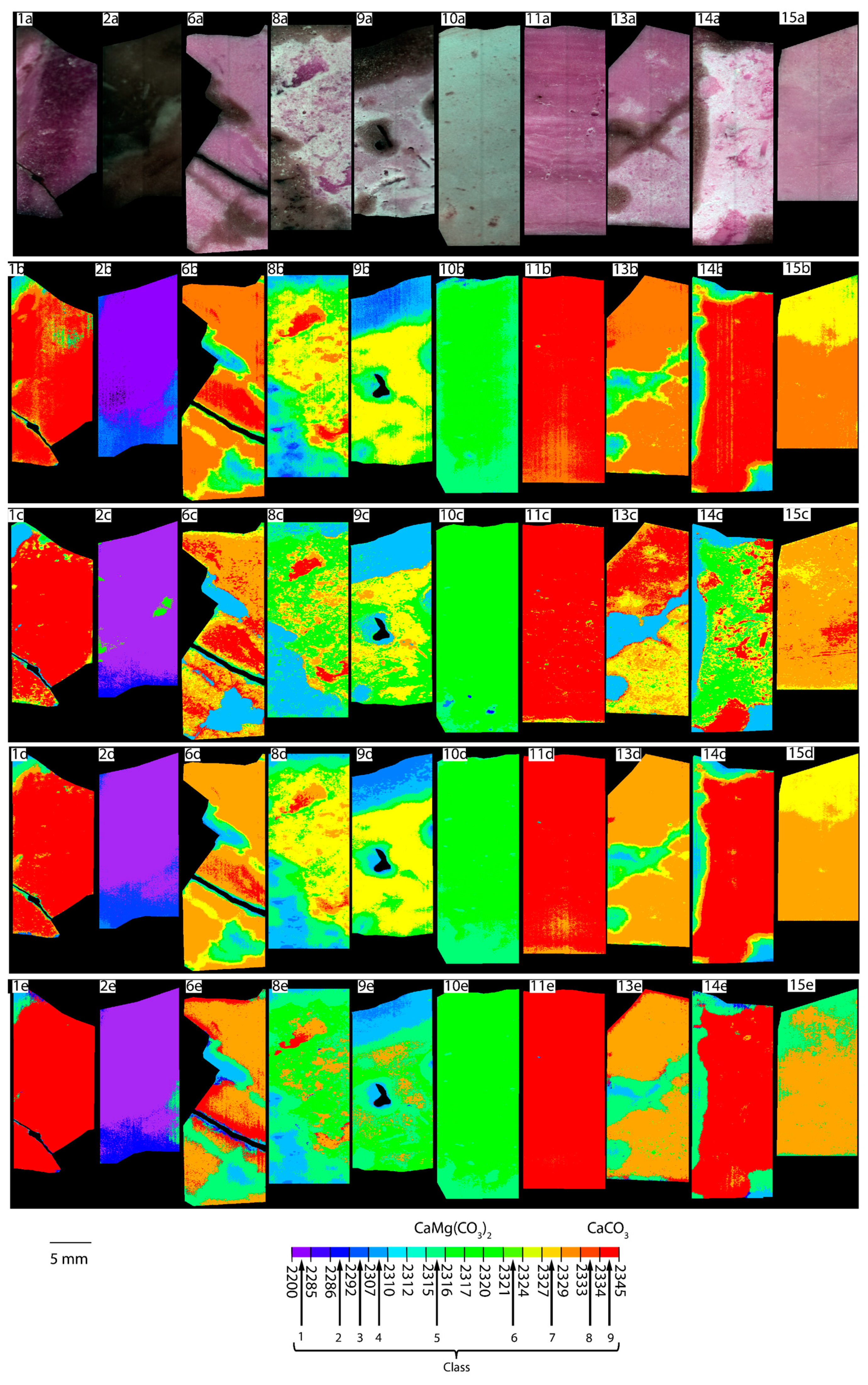
3.1. Edwards Formation, Central Texas, USA

Evaluation of mineral mixtures for absorption depth and minimum location between 2210 nm and 2400 nm has revealed relationships between mineral abundances and spectral characteristics (Figure 4). A higher abundance of calcite is most correlated with the absorption band center at longer wavelengths, and the highest abundance of chert is related to lower absorption depth in this spectral region.
Thresholds were set for abundances of calcite, dolomite, and chert were established from mineral mixtures that were prepared in the laboratory (Table 1); these were used to classify rock chips based on rock/mineral proportions. Differences in abundance range from 0.2% to 18% for calcite, 1% to 26% for dolomite, and 0 to 23% for chert. There are several explanations for the differences in abundance between point counts and HSI mapping. Point counts were conducted using high-resolution microscopy, where objects smaller than a micrometer could be resolved at the highest magnification. Additionally, spectral measurements were made on the other half of each rock slab, which could account for some of the variability in composition. The use of mineral mixtures for setting thresholds for mineral classification introduces errors in measurement and from sensor noise. In the scanned mineral mixtures, weak correlations between minimum wavelength position and abundance of calcite and silica, but no correlation with dolomite abundance were observed (Figure 5). Mineral maps produced from absorption band centers had mineral abundances that correlated with abundances obtained from point counting (Figure 6), with endmembers extracted for certain absorption band centers (Figure 7). High-resolution laboratory scanning of limestone, dolostone, and chert samples from the Edwards formation was used for detailed mineral abundance prediction using the position of the carbonate absorption minimum location (Figure 8).
The minimum wavelength image was used to generate a random sample of 300 pixels per class for training the SAM, SVM, and Neural Net classifiers. Classification accuracies were compared using confusion matrices [66], with the absorption band center image as reference. For the Edwards Limestone samples, SVM classified the carbonate samples with greater accuracy (84.4%) and kappa coefficient (0.82) than SAM and Neural Network (56.2%; 0.48 and 66.4%; 0.59, respectively). The aim was to distinguish materials that were not spectrally distinct with only minute differences in absorption locations, and similar overall spectral shapes. Because SVM is optimized to define functions based on training data situated near decision boundaries [67], it is likely the most accurate technique of the three that were attempted to separate spectrally similar classes. SVM has previously been used to classify clays and carbonates materials in hyperspectral imagery [68] and was applied to petrophysical logs to characterize carbonate reservoir facies [69]. SAM had the lowest overall accuracy, likely due to its reliance on curve shape for class separation.
Laboratory-based HSI can provide estimates of mineral abundance that are comparable to point counting (Figure 6), although both techniques suffer from certain shortcomings. HSI data are prone to sensor noise and require subsequent data processing to correct image artifacts and convert to reflectance for comparison to spectral library standards. Furthermore, the lack of distinguishing spectral features of some mineral groups in SWIR wavelengths makes the approach used in the present study unreliable for those minerals. This technique is suitable for distinguishing various carbonate, clay, hydroxide, sulfate, and other minerals, as well as hydrocarbons and other materials. Mapping the mineralogy of veins and microstructures can be useful for geologic studies [70,71] and can be achieved in a more extensive fashion using HSI than traditional techniques. Point counting introduces errors due to user interpretation, grid distance, and grain transition boundaries [72], and thin section preparation can be time consuming. However, this method has the advantage of high-resolution observation for studying diagenesis and other phenomena.

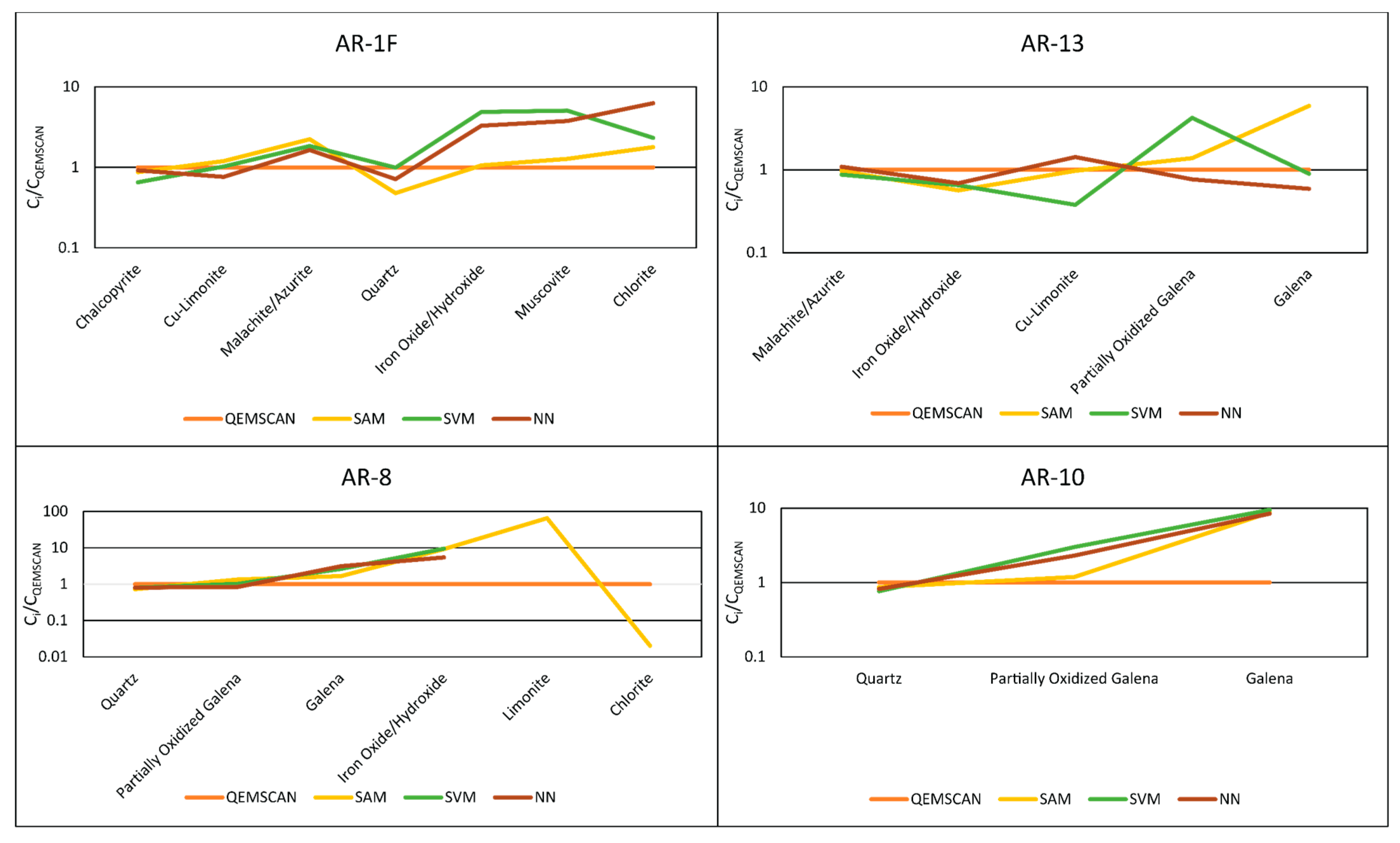
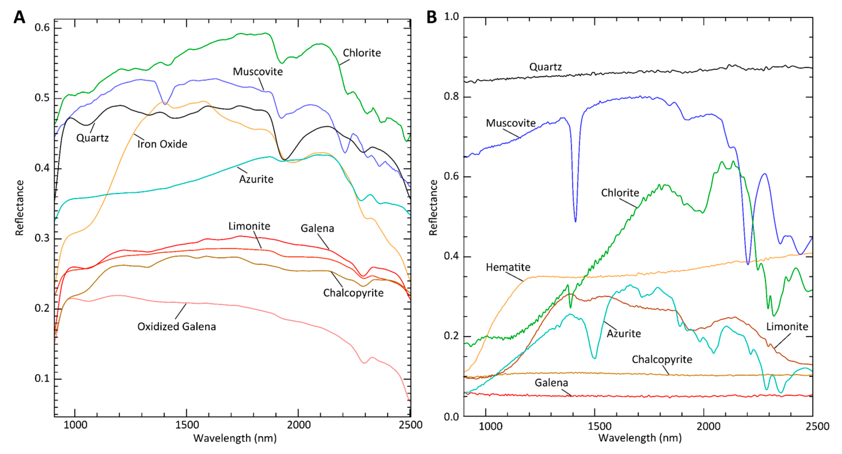
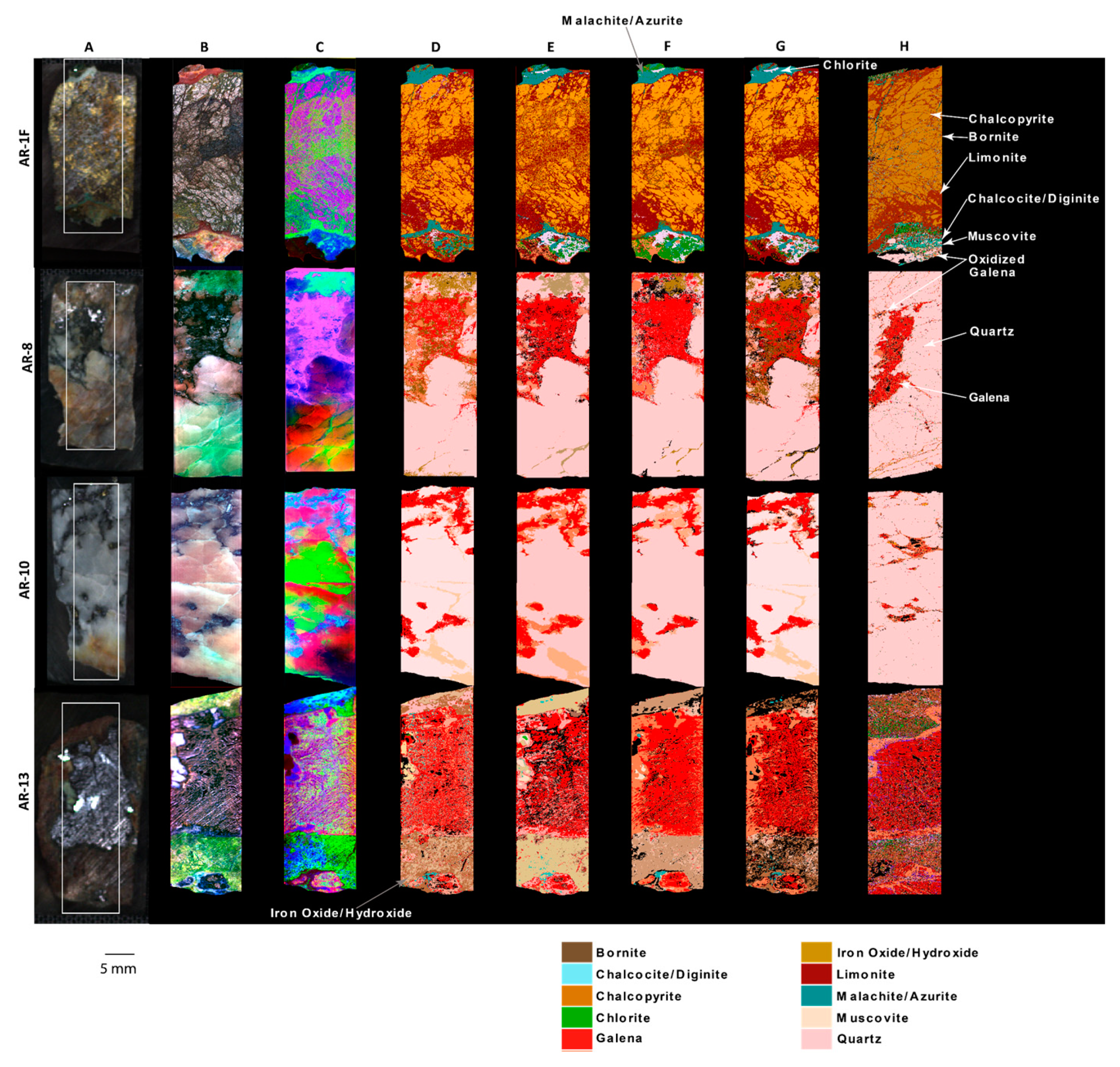
3.2. Sulfide-Rich Quartz Veins from Ladakh Batholith, Northern Pakistan

This work aims to test the feasibility of mapping sulfide minerals using imaging spectroscopy by validation using QEMSCAN mineral maps. Detection of sulfide minerals such as pyrite and chalcopyrite in the SWIR spectral region presents a challenge, because these opaque minerals have low overall reflectance and diminish spectral features of other minerals [48]. This work compared hyperspectral mineral classification to QEMSCAN data, also evaluating the suitability of commonly used classification techniques.
Mineral maps and abundances from each classification technique and QEMSCAN abundances that were derived from a subset image that was resampled to hyperspectral image resolution are presented as are differences in these abundances (Table 2, Figure 9). Spectra from the images (Figure 10A) and spectral libraries (Figure 10B) [36] are compared. Sample AR-1F showed the greatest similarity to QEMSCAN mineral abundances with SAM and Neural Net classification, although SVM results were least similar to abundances in the reference data (Table 2, Figure 9). SAM has been useful for classifying sulfide minerals [21,73], including underwater applications under artificial illumination [74,75].
Sample AR-13 shows a relatively accurate classification of galena, but significant differences in classification of oxidized galena. Although SAM outperforms SVM and Neural Net for classification of limonite, iron oxide is most accurately classified by Neural Net, and azurite by SVM. Samples AR-8 and AR-10 show substantial differences between QEMSCAN and classified abundances of quartz, galena, and limonite. Lack of consistency or similarity of classification results to QEMSAN data may be attributed to inaccuracy of the technique and endmember selection but is also likely a result of compositional offset resulting from sample preparation. Classification results that produced abundance that is closest to resampled QEMSCAN abundance were combined (Figure 11G) to produce mineral maps that have the closest resemblance to the reference images.
It is visible that samples AR-8 and AR-10 have a much higher proportion of galena and oxidized galena than the other half that was sent for QEMSCAN analysis. Furthermore, galena, limonite, and chalcopyrite have similar spectral curves in these samples (Figure 11A), making them a challenge to distinguish. These may be misclassified because only minute differences in spectral shape exist between these minerals.
Error distance was calculated (Table 3) using the following formula (Equation (1)):
ε | χ | j = 1 m i = 1 m | C j i C Q E M S C A N i | C Q E M S C A N i
where j = SAM, SVM, and NN is compared to QEMSCAN abundances, and i is the composition of each mineral.
Geochemical techniques and microscopy are commonly used for characterizing mineralogy, but reflectance spectroscopy may provide a less expensive alternative. Although imaging spectroscopy does not yet achieve the spatial resolution, reliability, and repeatability of techniques such as QEMSCAN, it can be used for sample logging at a higher speed. It is reported that at 10 µm resolution, 3 cm2 can be analyzed within approximately 3 h [76]. Within that time frame, about five times that area or more could be scanned and analyzed using HSI at approximately 30 µm resolution.

4. Conclusions

This work compared high-resolution laboratory imaging spectroscopy to mineral quantification using petrography and QEMSCAN for sample suites of two compositional endmembers. Spectral libraries from prepared mineral mixtures were used to set minimum wavelength thresholds for carbonate minerals and to train several classification algorithms. SAM, SVM, and Neural Network classifiers were compared, finding SVM yielded the highest accuracy for classifying carbonates. Classification of sulfide samples was compared to QEMSCAN mineral mapping, finding SAM showed the greatest similarity. It is possible that the SVM technique had better performance in classifying carbonates due to its ability to distinguish spectrally similar materials, whereas SAM had higher accuracy in classifying sulfides due to the differences in the overall shape of the mineral spectral reflectance curves. Additional work using different mineral phases and directly comparable validation data could provide more clarity on the advantages and drawbacks of commonly used classification techniques when applied to high resolution laboratory SWIR imaging.

Author Contributions

Conceptualization by D.K. and S.D.K., Writing—Original Draft Preparation by D.K.; remote sensing data processing by D.K.; writing—review and editing, D.K. and S.D.K.; supervision and funding acquisition S.D.K. All authors have read and agreed to the published version of the manuscript.

Funding

This research received no external funding. Sample sin Astore are of Pakistan were collected by project funded by the National Academy of Science.

Acknowledgments

Authors thank Laeiq Ahmad and M.T. Shah for sample collection in the Astore area. Charlotte Sylvan helped in sampling at Lake George Town.

Conflicts of Interest

The authors declare no conflict of interest.

References

  1. Dale, L.M.; Thewis, A.; Boudry, C.; Rotar, I.; Dardenne, P.; Baeten, V.; Pierna, J.A.F. Hyperspectral Imaging Applications in Agriculture and Agro-Food Product Quality and Safety Control: A Review. Appl. Spectrosc. Rev. 2013, 48, 142–159. [Google Scholar] [CrossRef]
  2. Ishida, T.; Kurihara, J.; Viray, F.A.; Namuco, S.B.; Paringit, E.C.; Perez, G.J.; Takahashi, Y.; Marciano, J.J. A novel approach for vegetation classification using UAV-based hyperspectral imaging. Comput. Electron. Agric. 2018, 144, 80–85. [Google Scholar] [CrossRef]
  3. Huang, H.; Liu, L.; Ngadi, M.O. Recent developments in hyperspectral imaging for assessment of food quality and safety. Sensors 2014, 14, 7248–7276. [Google Scholar] [CrossRef] [PubMed] [Green Version]
  4. Park, B.; Yoon, S.-C.; Windham, W.R.; Lawrence, K.C.; Kim, M.S.; Chao, K. Line-scan hyperspectral imaging for real-time in-line poultry fecal detection. Sens. Instrum. Food Qual. Saf. 2011, 5, 25–32. [Google Scholar] [CrossRef]
  5. Calin, M.A.; Parasca, S.V.; Savastru, D.; Manea, D. Hyperspectral Imaging in the Medical Field: Present and Future. Appl. Spectrosc. Rev. 2013, 49, 435–447. [Google Scholar] [CrossRef]
  6. Johnson, W.R.; Wilson, D.W.; Fink, W.; Humayun, M.; Bearman, G. Snapshot hyperspectral imaging in ophthalmology. J. Biomed. Opt. 2007, 12, 014036. [Google Scholar] [CrossRef] [Green Version]
  7. Payne, G.; Wallace, C.; Reedy, B.; Lennard, C.; Schuler, R.; Exline, D.; Roux, C. Visible and near-infrared chemical imaging methods for the analysis of selected forensic samples. Talanta 2005, 67, 334–344. [Google Scholar] [CrossRef]
  8. Edelman, G.; van Leeuwen, T.G.; Aalders, M.C. Hyperspectral imaging for the age estimation of blood stains at the crime scene. Forensic Sci. Int. 2012, 223, 72–77. [Google Scholar] [CrossRef]
  9. Leask, E.K.; Ehlmann, B.L. Identifying and quantifying mineral abundance through VSWIR microimaging spectroscopy: A comparison to XRD and SEM. In Proceedings of the 8th Workshop on Hyperspectral Image and Signal Processing: Evolution in Remote Sensing (WHISPERS), Los Angeles, CA, USA, 21–24 August 2016. [Google Scholar]
  10. Boesche, N.; Rogass, C.; Lubitz, C.; Brell, M.; Herrmann, S.; Mielke, C.; Tonn, S.; Appelt, O.; Altenberger, U.; Kaufmann, H. Hyperspectral REE (Rare Earth Element) Mapping of Outcrops—Applications for Neodymium Detection. Remote Sens. 2015, 7, 5160–5186. [Google Scholar] [CrossRef] [Green Version]
  11. Koerting, F.; Rogass, C.; Kaempf, H.; Lubitz, C.; Harms, U.; Schudack, M.; Kokaly, R.; Mielke, C.; Boesche, N.; Altenberger, U. Drill core mineral analysis by means of the hyperspectral imaging spectrometer HySpex, XRD and ASD in proximity of the Mýtina Maar, Czech Republic. ISPRS Int. Arch. Photogramm. Remote Sens. Spat. Inf. Sci. 2015, XL-1-W5, 417–424. [Google Scholar] [CrossRef] [Green Version]
  12. Rogass, C.; Koerting, F.M.; Mielke, C.; Brell, M.; Boesche, N.K.; Bade, M.; Hohmann, C. Translational Imaging Spectroscopy for Proximal Sensing. Sensors 2017, 17, 1857. [Google Scholar] [CrossRef] [Green Version]
  13. Krupnik, D.; Khan, S.D. Close-range, ground-based hyperspectral imaging for mining applications at various scales: Review and case studies. Earth Sci. Rev. 2019, 198, 102952. [Google Scholar] [CrossRef]
  14. Polak, A.; Kelman, T.; Murray, P.; Marshall, S.; Stothard, D.J.M.; Eastaugh, N.; Eastaugh, F. Hyperspectral imaging combined with data classification techniques as an aid for artwork authentication. J. Cult. Herit. 2017, 26, 1–11. [Google Scholar] [CrossRef]
  15. Ferreira, K.B.; Oliveira, A.G.G.; Gonçalves, A.S.; Gomes, J.A. Evaluation of Hyperspectral Imaging Visible/Near Infrared Spectroscopy as a forensic tool for automotive paint distinction. Forensic Chem. 2017, 5, 46–52. [Google Scholar] [CrossRef]
  16. Khan, M.J.; Khan, H.S.; Yousaf, A.; Khurshid, K.; Abbas, A. Modern Trends in Hyperspectral Image Analysis: A Review. IEEE Access 2018, 6, 14118–14129. [Google Scholar] [CrossRef]
  17. Adep, R.N.; shetty, A.; Ramesh, H. EXhype: A tool for mineral classification using hyperspectral data. ISPRS J. Photogramm. Remote Sens. 2017, 124, 106–118. [Google Scholar] [CrossRef]
  18. Schneider, S.; Melkumyan, A.; Murphy, R.J.; Nettleton, E. Gaussian processes with OAD covariance function for hyperspectral data classification. In Proceedings of the 2010 22nd IEEE International Conference on Tools with Artificial Intelligence, Arras, France, 27–29 October 2010; pp. 393–400. [Google Scholar]
  19. Pal, M.; Rasmussen, T.; Porwal, A. Optimized Lithological Mapping from Multispectral and Hyperspectral Remote Sensing Images Using Fused Multi-Classifiers. Remote Sens. 2020, 12, 177. [Google Scholar] [CrossRef] [Green Version]
  20. Maity, A. Supervised Classification of RADARSAT-2 Polarimetric Data for Different Land Features. arXiv 2016, arXiv:1608.00501. [Google Scholar]
  21. Bolin, B.J.; Moon, T.S. Sulfide detection in drill core from the Stillwater Complex using visible/near-infrared imaging spectroscopy. Geophysics 2003, 68, 1561–1568. [Google Scholar] [CrossRef]
  22. Scafutto, R.D.P.M.; Souza Filho, C.R.d.; Rivard, B. Characterization of mineral substrates impregnated with crude oils using proximal infrared hyperspectral imaging. Remote Sens. Environ. 2016, 179, 116–130. [Google Scholar] [CrossRef]
  23. Lancelot, E.; Bertrand, D.; Hanafi, M.; Jaillais, B. Near-infrared hyperspectral imaging for following imbibition of single wheat kernel sections. Vib. Spectrosc. 2017, 92, 46–53. [Google Scholar] [CrossRef]
  24. Mäkelä, M.; Volpe, M.; Volpe, R.; Fiori, L.; Dahl, O. Spatially resolved spectral determination of polysaccharides in hydrothermally carbonized biomass. Green Chem. 2018, 20, 1114–1120. [Google Scholar] [CrossRef] [Green Version]
  25. Dalm, M.; Buxton, M.W.N.; van Ruitenbeek, F.J.A. Discriminating ore and waste in a porphyry copper deposit using short-wavelength infrared (SWIR) hyperspectral imagery. Miner. Eng. 2017, 105, 10–18. [Google Scholar] [CrossRef]
  26. Buddenbaum, H.; Steffens, M. The Effects of Spectral Pretreatments on Chemometric Analyses of Soil Profiles Using Laboratory Imaging Spectroscopy. Appl. Environ. Soil Sci. 2012, 2012, 1–12. [Google Scholar] [CrossRef] [Green Version]
  27. Speta, M.; Rivard, B.; Feng, J.; Lipsett, M.; Gingras, M. Hyperspectral imaging for the determination of bitumen content in Athabasca oil sands core samples. AAPG Bull. 2015, 99, 1245–1259. [Google Scholar] [CrossRef]
  28. Demirmen, F. Counting error in petrographic point-count analysis: A theoretical and experimental study. J. Int. Assoc. Math. Geol. 1971, 3, 15–41. [Google Scholar] [CrossRef]
  29. Zhang, X.; Liu, B.; Wang, J.; Zhang, Z.; Shi, K.; Wu, S. Adobe photoshop quantification (PSQ) rather than point-counting: A rapid and precise method for quantifying rock textural data and porosities. Comput. Geosci. 2014, 69, 62–71. [Google Scholar] [CrossRef]
  30. Contreras Acosta, I.; Khodadadzadeh, M.; Tusa, L.; Ghamisi, P.; Gloaguen, R. A Machine Learning Framework for Drill-Core Mineral Mapping Using Hyperspectral and High-Resolution Mineralogical Data Fusion. IEEE J. Sel. Top. Appl. Earth Obs. Remote Sens. 2019, 1–14. [Google Scholar] [CrossRef]
  31. Laakso, K.; Middleton, M.; Heinig, T.; Bärs, R.; Lintinen, P. Assessing the ability to combine hyperspectral imaging (HSI) data with Mineral Liberation Analyzer (MLA) data to characterize phosphate rocks. Int. J. Appl. Earth Obs. Geoinf. 2018, 69, 1–12. [Google Scholar] [CrossRef]
  32. Zaini, N.; Van Der Meer, F.D.; Van Der Werff, H. Effect of Grain Size and Mineral Mixing on Carbonate Absorption Features in the SWIR and TIR Wavelength Regions. Remote. Sens. 2012, 4, 987–1003. [Google Scholar] [CrossRef] [Green Version]
  33. Krupnik, D.; Khan, S.; Okyay, U.; Hartzell, P.; Zhou, H.-W. Study of Upper Albian rudist buildups in the Edwards Formation using ground-based hyperspectral imaging and terrestrial laser scanning. Sediment. Geol. 2016, 345, 154–167. [Google Scholar] [CrossRef] [Green Version]
  34. Ahmad, L.; Khan, S.D.; Shah, M.T.; Jehan, N. Gold mineralization in Bubin area, Gilgit-Baltistan, Northern Areas, Pakistan. Arab. J. Geosci. 2018, 11, 18. [Google Scholar] [CrossRef]
  35. Khan, S.D.; Okyay, U.; Ahmad, L.; Shah, M.T. Characterization of Gold Mineralization in Northern Pakistan Using Imaging Spectroscopy. Photogramm. Eng. Remote. Sens. 2018, 84, 425–434. [Google Scholar] [CrossRef]
  36. Clark, R.N.; Swayze, G.A.; Wise, R.; Livo, E.; Hoefen, T.; Koklay, R.F.; Sutley, S.J. USGS Digital Spectral Library Splib06a; United States Geological Survey: Reston, VA, USA, 2007.
  37. Clark, R.N.; Gallagher, A.J.; Swayze, G.A. Material absorption band depth mapping of imaging spectrometer data using a complete band shape least-squares fit with library reference spectra. In Proceedings of the Second Airborne Visible/Infrared Imaging Spectrometer (AVIRIS); Jet Propulsion Laboratory, California Institute of Technology: Pasadena, CA, USA, 1990; pp. 176–186. [Google Scholar]
  38. Cloutis, E.A.; Hawthorne, F.C.; Mertzman, S.A.; Krenn, K.; Craig, M.A.; Marcino, D.; Methot, M.; Strong, J.; Mustard, J.F.; Blaney, D.L.; et al. Detection and discrimination of sulfate minerals using reflectance spectroscopy. Icarus 2006, 184, 121–157. [Google Scholar] [CrossRef]
  39. Mustard, J.F. Chemical analysis of actinolite from reflectance spectra. Am. Mineral. 1992, 77, 345–358. [Google Scholar]
  40. Cloutis, E.A.; Gaffey, M.J.; Moslow, T.F. Spectral reflectance properties of carbon-bearing materials. Icarus 1994, 107, 276–287. [Google Scholar] [CrossRef]
  41. Baissa, R.; Labbassi, K.; Launeau, P.; Gaudin, A.; Ouajhain, B. Using HySpex SWIR-320m hyperspectral data for the identification and mapping of minerals in hand specimens of carbonate rocks from the Ankloute Formation (Agadir Basin, Western Morocco). J. Afr. Earth Sci. 2011, 61, 1–9. [Google Scholar] [CrossRef]
  42. Clark, R.N. Spectroscopy of Rocks and Minerals, and Principles of Spectroscopy. In Manual of Remote Sensing; Rencz, A.N., Ed.; John Wiley and Sons Inc.: New York, NY, USA, 1999; pp. 3–58. [Google Scholar]
  43. Van der Meer, F. Spectral Reflectance of Carbonate Mineral Mixtures and Bidirectional Reflectance Theory: Quantitative Analysis techniques for Application in Remote Sensing. Remote Sens. Rev. 1995, 13, 67–94. [Google Scholar] [CrossRef]
  44. Crowley, J.K. Visible and near-infrared spectra of carbonate rocks: Reflectance variations related to petrographic texture and impurities. J. Geophys. Res. 1986, 91, 5001. [Google Scholar] [CrossRef]
  45. Zaini, N.; van der Meer, F.; van der Werff, H. Determination of Carbonate Rock Chemistry Using Laboratory-Based Hyperspectral Imagery. Remote Sens. 2014, 6, 4149–4172. [Google Scholar] [CrossRef] [Green Version]
  46. Hunt, G.R. Spectroscopic properties of rocks and minerals. In Handbook of Physical Properties of Rocks; CRC Press: Boca Raton, FL, USA, 1982; pp. 295–386. [Google Scholar]
  47. Gallie, E.A.; McArdle, S.; Rivard, B.; Francis, H. Estimating sulphide ore grade in broken rock using visible/infrared hyperspectral reflectance spectra. Int. J. Remote Sens. 2002, 23, 2229–2246. [Google Scholar] [CrossRef]
  48. Hunt, G.R. Visible and near-infrared spectra of minerals and rocks: IV. Sulphides and sulphates. Mod. Geol. 1971, 3, 1–14. [Google Scholar]
  49. Van der Werff, H. IDL DISPEC 3.6; ITC: Enschede, The Netherlands, 2007. [Google Scholar]
  50. Smith, G.M.; Milton, E.J. The use of the empirical line method to calibrate remotely sensed data to reflectance. Int. J. Remote Sens. 1999, 20, 2653–2662. [Google Scholar] [CrossRef]
  51. Harris Geospatial. Bad Data Mitigation Tools. Available online: https://www.harrisgeospatial.com/docs/THORBadDataTools.html (accessed on 9 May 2020).
  52. Bromba, M.U.A.; Ziegler, H. Application hints for Savitzky-Golay digital smoothing filters. Anal. Chem. 1981, 53, 1583–1586. [Google Scholar] [CrossRef]
  53. Savitzky, A.; Golay, M.J.E. Smoothing and Differentiation of Data by Simplified Least Squares Procedures. Anal. Chem. 1964, 36, 1627–1639. [Google Scholar] [CrossRef]
  54. Crowley, J.K.; Brickey, D.W.; Rowan, L.C. Airborne imaging spectrometer data of the Ruby Mountains, Montana: Mineral discrimination using relative absorption band-depth images. Remote Sens. Environ. 1989, 29, 121–134. [Google Scholar] [CrossRef]
  55. Sun, L.; Khan, S.; Godet, A. Integrated ground-based hyperspectral imaging and geochemical study of the Eagle Ford Group in West Texas. Sediment. Geol. 2018, 363, 34–47. [Google Scholar] [CrossRef]
  56. Van der Meer, F. Sequential indicator conditional simulation and indicator kriging applied to discrimination of dolomitization in GER 63-channel imaging spectrometer data. Nonrenewable Resour. 1994, 3, 146–164. [Google Scholar]
  57. Bakker, W.H. HypPy User Manual: Graphical User-Interface (GUI); ITC: Enschede, The Netherlands, 2012. [Google Scholar]
  58. Kruse, F.A.; Lefkoff, A.B.; Boardman, J.W.; Heidebrecht, K.B.; Shapiro, A.T.; Barloon, P.J.; Goetz, A.F.H. The spectral image processing system (SIPS)—Interactive visualization and analysis of imaging spectrometer data. Remote Sens. Environ. 1993, 44, 145–163. [Google Scholar] [CrossRef]
  59. Richards, J.A.; Jia, X. Remote Sensing Digital Image Analysis; Springer: Berlin/Heidelberg, Germany, 1999; Volume 3. [Google Scholar]
  60. Wu, T.-F.; Lin, C.-J.; Weng, R.C. Probability Estimates for Multi-class Classification by Pairwise Coupling. J. Mach. Learn. Res. 2004, 5, 975–1005. [Google Scholar]
  61. Vapnik, V. The Nature of Statistical Learning Theory; Springer Science & Business Media: New York, NY, USA, 2013. [Google Scholar]
  62. Monteiro, S.T.; Murphy, R.J. Calibrating probabilities for hyperspectral classification of rock types. In Proceedings of the 2010 IEEE International Geoscience and Remote Sensing Symposium (IGARSS), Honolulu, HI, USA, 25–30 July 2010; pp. 2800–2803. [Google Scholar]
  63. Murphy, R.J.; Monteiro, S.T.; Schneider, S. Evaluating Classification Techniques for Mapping Vertical Geology Using Field-Based Hyperspectral Sensors. IEEE Trans. Geosci. Remote Sens. 2012, 50, 3066–3080. [Google Scholar] [CrossRef]
  64. Chopard, A.; Marion, P.; Royer, J.-J.; Taza, R.; Bouzahzah, H.; Benzaazoua, M. Automated sulfides quantification by multispectral optical microscopy. Miner. Eng. 2019, 131, 38–50. [Google Scholar] [CrossRef]
  65. Harris Geospatial Solutions. Neural Net. Available online: https://www.harrisgeospatial.com/docs/NeuralNet.html (accessed on 25 October 2019).
  66. Lewis, H.G.; Brown, M. A generalized confusion matrix for assessing area estimates from remotely sensed data. Int. J. Remote Sens. 2010, 22, 3223–3235. [Google Scholar] [CrossRef]
  67. Melgani, F.; Bruzzone, L. Classification of hyperspectral remote sensing images with support vector machines. IEEE Trans. Geosci. Remote Sens. 2004, 42, 1778–1790. [Google Scholar] [CrossRef] [Green Version]
  68. Gasmi, A.; Zouari, H.; Masse, A.; Ducrot, D. Potential of the Support Vector Machine (SVMs) for clay and calcium carbonate content classification from hyperspectral remote sensing. Int. J. Innov. Appl. Stud. 2015, 13, 497–506. [Google Scholar]
  69. Sebtosheikh, M.A.; Motafakkerfard, R.; Riahi, M.A.; Moradi, S. Separating Well Log Data to Train Support Vector Machines for Lithology Prediction in a Heterogeneous Carbonate Reservoir. Iran. J. Oil Gas. Sci. Technol. 2015, 4, 1–14. [Google Scholar]
  70. Van Ruitenbeek, F.J.A.; van der Werff, H.M.A.; Bakker, W.H.; van der Meer, F.D.; Hein, K.A.A. Measuring rock microstructure in hyperspectral mineral maps. Remote Sens. Environ. 2019, 220, 94–109. [Google Scholar] [CrossRef]
  71. Tusa, L.; Andreani, L.; Khodadadzadeh, M.; Contreras, C.; Ivascanu, P.; Gloaguen, R.; Gutzmer, J. Mineral Mapping and Vein Detection in Hyperspectral Drill-Core Scans: Application to Porphyry-Type Mineralization. Minerals 2019, 9, 122. [Google Scholar] [CrossRef] [Green Version]
  72. Neilson, M.J.; Brockman, G.F. The error associated with point-counting. Am. Mineral. 1977, 62, 1238–1244. [Google Scholar]
  73. Rammlmair, D.; Meima, J. Quantitative mineralogy of chromite ore based on imaging Laser Induced Breakdown Spectroscopy and Spectral Angle Mapper Classification Algorithm. In Proceedings of the EGU General Assembly, Vienna, Austria, 4–8 May 2020. [Google Scholar]
  74. Dumke, I.; Nornes, S.M.; Purser, A.; Marcon, Y.; Ludvigsen, M.; Ellefmo, S.L.; Johnsen, G.; Søreide, F. First hyperspectral imaging survey of the deep seafloor: High-resolution mapping of manganese nodules. Remote Sens. Environ. 2018, 209, 19–30. [Google Scholar] [CrossRef]
  75. Sture, Ø.; Ludvigsen, M.; Aas, L.M.S. Autonomous underwater vehicles as a platform for underwater hyperspectral imaging. In Proceedings of the OCEANS 2017, Aberdeen, UK, 19–22 June 2017; pp. 1–8. [Google Scholar]
  76. Ayling, B.; Rose, P.; Petty, S.; Zemach, E.; Drakos, P. QEMSCAN (Quantitative evaluation of minerals by scanning electron microscopy): Capability and application to fracture characterization in geothermal systems. In Proceedings of the 37th Workshop on Geothermal Reservoir Engineering 2012, Stanford, CA, USA, 30 January–1 February 2012. [Google Scholar]
Figure 1. (A) Study location in Google Earth, modified from [33]. (B) Rock chip sample locations along the outcrop, the background is LiDAR-derived topography textured with a false-color composite of 2378, 2334, and 2146 nm in RGB, data from [33].
Minerals 10 00967 g001
Figure 2. Geologic map of the Astor area in Northern Pakistan. Bulk samples were collected from the Astore area. Modified from [35].
Minerals 10 00967 g002
Figure 3. Spectral absorption feature characteristics modified after [25].
Minerals 10 00967 g003
Figure 4. Absorption minimum maps of mixtures prepared in the laboratory (abundances shown in Table 1). Sample numbers refer to Table 1.
Minerals 10 00967 g004
Figure 5. Minimum wavelength locations and depths of prepared mixtures measured from hyperspectral imagery, compared to mineral proportions by weight. Error bars show standard deviation of measurements.
Minerals 10 00967 g005
Figure 6. (A) Comparison of mineral abundances from point count in comparison to pixels counted from HSI-derived mineral maps using absorption minimum location, and (B) graphs that compare the abundances of each mineral with HSI on the y-axis and point counting on the x-axis.
Minerals 10 00967 g006
Figure 7. Endmember spectral plots from each class mapped in Figure 8. Sample numbers refer to Table 1.
Minerals 10 00967 g007
Figure 8. Rock chips from the Lake Georgetown spillway: (115a) in 2102, 2334, and 2397 nm RGB false color composites and (115b) with minimum wavelength positions mapped. (115c) spectral angle mapper, (115d) support vector machine, and (115e) Neural Network classifications.
Minerals 10 00967 g008
Figure 9. Comparison of compositions obtained by different classification techniques. The ratio of the composition obtained by each technique to the abundance determined by QEMSCAN is shown—Ci/CQEMSCAN (i = SAM, SVM, NN) A log scale is used for the y-axis.
Minerals 10 00967 g009
Figure 10. Endmember spectral plots from each class that was mapped in Figure 11, (A) derived from hyperspectral data and (B) from the USGS spectral library [36].
Minerals 10 00967 g010
Figure 11. Sulfide samples (A) True color composite with the high-resolution scan area outlined in white. (B) SWIR false color composite AR1-F: 2102, 1359, 953 nm; AR-8: 934, 1819, 2447 nm; AR-10: 934, 1819, 2447 nm; and AR-13: 2453, 1794, 966 nm. (C) MNF color composites AR1-F: 1, 3, 2 AR-8 and AR-10: 3, 2, 1; and AR-13: 1, 2, 4. (D) SAM, (E) SVM, and (F) Neural Net classifications. (G) A combination of classes that most closely match QEMSCAN abundances, as shown by outlined cells of Table 2. (H) QEMSCAN image that has been subset to approximately the same extent as the hyperspectral imagery. Legend colors apply to images D–H. The scale bar applies to B–H.
Minerals 10 00967 g011
Table 1. Mineral abundances (by mass) and mean absorption minimum locations measured from hyperspectral imaging (HSI).
Sample Number% Calcite% Dolomite% ChertMean Min Wavelength (nm)Mean Depth (%)
110000233721.14
201000230910.24
30010022844.95
40257522865.95
50505022896.33
60752522997.63
725750231311.25
850500232112.99
975250233215.09
102507522865.69
115005023353.07
122507522861.91
1315157022872.13
1415355023113.43
1525255023172.98
1635155023273
1733333323234.26
1825502523195.22
1950252523285.14
2015701523165.98
2170151523348.71
Table 2. Mineral abundances from selected sulfide samples. The number below each classified percentage in parentheses indicates the difference between QEMSCAN and classification abundance. Classes with abundances that are closest to QEMSCAN proportions are outlined.
Mineral/GroupQEMSCANSAMSVMNeural NetMineral/GroupQEMSCANSAMSVMNeural Net
%%%%%%%%
AR-1FChalcopyrite49.6943.29
(−6.4)
32.5
(−17.2)
45.6
(−4.1)
AR-13Galena41.6840
(−1.7)
36.3
(−5.4)
45.3
(3.6)
Cu-Limonite34.5841.4
(6.8)
35.3
(0.8)
26.4
(−8.2)
Partially Oxidized Galena31.517.65
(−13.8)
20.4
(−11.2)
21.5
(−10)
Malachite/Azurite3.197.14
(3.95)
5.86
(2.7)
5.2
(2.03)
Limonite17.917.24
(−0.6)
6.7
(−11.1)
25.4
(7.52)
Quartz4.42.11
(−2.3)
4.4
(0)
3.2
(−1.3)
Iron Oxide/Hydroxide8.211.23
(3.06)
34.6
(26.4)
6.3
(−1.9)
Iron Oxide/Hydroxide3.53.7
(0.19)
16.9
(13.4)
11.4
(8)
Malachite/Azurite0.84.63
(3.84)
0.70
(−0.09)
0.5
(−0.3)
Bornite2Muscovite9.191.261.1
Chalcocite/Diginite1.1Chlorite0.10.10
Muscovite0.60.7
(0.2)
2.8
(2.3)
2.1
(1.6)
Chlorite11.72
(0.8)
2.3
(1.3)
6.1
(5.1)
Mineral/GroupQEMSCANSAMSVMNeural NetMineral/GroupQEMSCANSAMSVMNeural Net
%%%%%%%%
AR-8Quartz84.160.6
(−23.5)
66.7
(−17.4)
66.5
(−17.6)
AR-10Quartz93.580.7
(−12.8)
71.6
(−21.9)
76.3
(−17.2)
Oxidized Galena6.58.7
(2.2)
6.6
(0.1)
5.4
(−1.1)
Partially Oxidized Galena4.45.2
(0.8)
13.2
(8.8)
10.2
(5.8)
Galena813.2
(5.2)
21
(13)
24.8
(16.8)
Galena1.614.1
(12.5)
15.3
(13.7)
13.6
(12)
Iron Oxide/Hydroxide0.65.6
(4.97)
5.7
(5.1)
3.3
(2.7)
Chalcopyrite0.3
Limonite0.211.9
(11.7)
Chlorite0.2
Chlorite0.50
(0)
Table 3. Error distance for each sample.
Sample NumberSAMSVMNN
AR-1F0.461.501.65
AR-131.150.890.30
AR-82.352.551.71
AR-102.693.582.97
Publisher’s Note: MDPI stays neutral with regard to jurisdictional claims in published maps and institutional affiliations.

