Regional Geochemical Anomaly Identification Based on Multiple-Point Geostatistical Simulation and Local Singularity Analysis—A Case Study in Mila Mountain Region, Southern Tibet

Abstract

The smoothing effect of data interpolation could cause useful information loss in geochemical mapping, and the uncertainty assessment of geochemical anomaly could help to extract reasonable anomalies. In this paper, multiple-point geostatistical simulation and local singularity analysis (LSA) are proposed to identify regional geochemical anomalies and potential mineral resources areas. Taking Cu geochemical data in the Mila Mountain Region, southern Tibet, as an example, several conclusions were obtained: (1) geochemical mapping based on the direct sampling (DS) algorithm of multiple-point geostatistics can avoid the smoothing effect through geochemical pattern simulation; (2) 200 realizations generated by the direct sampling simulation reflect the uncertainty of an unsampled value, and the geochemical anomaly of each realization can be extracted by local singularity analysis, which shows geochemical anomaly uncertainty; (3) the singularity-quantile (S-Q) analysis method was used to determine the separation thresholds of E-type α, and uncertainty analysis was carried out on the copper anomaly to obtain the anomaly probability map, which should be more reasonable than the interpolation-based geochemical map for geochemical anomaly identification. According to the anomaly probability and favorable geological conditions in the study area, several potential mineral resource targets were preliminarily delineated to provide direction for subsequent mineral exploration.

1. Introduction

The weak anomaly extraction of geological and geochemical information has played an important role in discovering potential mineral deposits [1]. In regional geochemical data processing, the complex geological and geographical background may result in difficulties associated with geochemical anomaly extraction, where high element content values may not be associated with orebody, but some low content values are. Therefore, reasonable geochemical anomaly identification is one of the most important challenges of geochemical exploration [2].

The rasterization of regional geochemical data is a common process in geochemical data processing; the kriging method [3,4,5] and inverse distance weighting method (IDW) [6] are common rasterization methods. A key problem is that it is difficult for a simple mathematical function or a deterministic model to accurately describe the spatial variability of an element to infer the value at the unsampled location from limited or sparse geochemical exploration data [5,7,8,9,10,11,12], which will result in uncertainty in the spatial prediction. Increasing the sampling density can certainly improve the prediction accuracy [13], but a higher cost follows. Therefore, more attention should be paid to uncertainty in geochemical exploration that influences the results [14]. The geostatistical simulation method could overcome the smoothing effect caused by interpolation through spatial uncertainty modeling of an unsampled location. The geostatistical simulation method can generate equal probability realizations of target attribute values and assign values to the original sampling position. The simulation result can reflect the spatial variation of the target attribute more realistically. Recently, geostatistical simulation methods have been widely used in the quantitative uncertainty of the geological field [14,15,16,17,18,19].

The traditional geostatistical simulation method is based on the variogram and considers the correlation between two points in space only. As for complex geological backgrounds or elements’ spatial distribution patterns, more than two statistical points should be described. The multiple-point geostatistical simulation is a target-based simulation method, which focuses on multiple-point patterns in space and absorbs the advantages of traditional two-point geostatistics to better characterize the spatial variability and delineate the uncertainty of variables [20,21,22,23,24]. Relevant simulation algorithms include pixel-based simulations, such as the extended normal equations simulation (ENESIM) algorithm [20], the single normal equation simulation (SNESIM) algorithm [25], and direct sampling (DS) algorithm [26,27]; pattern-based simulations, such as the simulation of patterns (SIMPAT) algorithm [28]; the filter-based pattern simulation (FILTERSIM) algorithm [29], and the cross-correlation-based simulation (CCSIM) algorithm [30]. These methods have been effectively applied in reservoir simulation, hydrogeological modeling, porous media reconstruction, and other geoscience fields [31,32,33], but there are few applications related to geochemical exploration [17,34,35]. The main reason for this is that an appropriate training image (TI) is difficult to obtain through the complex geochemical element spatial distribution. Although the data themselves can be used as the training image, sometimes the corresponding matching patterns are also difficult to obtain.

In this paper, a hybrid method combining the direct sampling (DS) algorithm of multiple-point geostatistical simulation and local singularity analysis (LSA) is proposed to estimate Cu anomalies associated with copper mineralization based on stream sediment geochemical data in the so-called ”Mila Mountain Integrated Exploration Region” in Tibet, China.

2. Methodology

2.1. Direct Sampling Algorithm (DS)

Instead of using a variogram to describe spatial heterogeneous geometric features, multiple-point geostatistics aims to use hard data (drill hole data, etc.) as conditional data to extract spatial patterns from training images (TI) [32]. Therefore, the simulation results effectively reflect the conditional data, and can better reproduce the structure of the simulated target.

The direct sampling algorithm is a pixel-based multiple-point geostatistical algorithm, which is used to simulate random function $Z(x)$ [26,32].

Usually, the conditional data are assigned to the nearest grid node in the singular grid (SG), and the simulation is performed by accessing the remaining nodes in SG through the defined random path until all the grids are traversed [26].

In detail, this involves selecting $n$ closest grid nodes $\left\{x_1,x_2,\dots ,x_n\right\}$ to the successive location of $x$, computing its lag vectors $L=\left\{h_1,h_2,\dots ,h_n\right\}$, and defining the data event $d_n(x,L)=\left\{Z(x+h_1),Z(x+h_2),\dots ,Z(x+h_n)\right\}$. Meanwhile, the TI is randomly scanned to obtain the data event, $d_n(y,L)=\left\{Z(y+h_1),Z(y+h_2),\dots ,Z(y+h_n)\right\}$, for each location of $y$. When the distance between $d_n(x,L)$ and $d_n(y,L)$ is smaller than a predefined threshold $t$, the $Z(y)$ is taken as the best-match value assigned to $Z(x)$. Otherwise, a maximal scanning fraction $f$ is set to control the simulation implementation by adopting the $Z(y)$, which has the lowest distance between $d_n(x,L)$ and $d_n(y,L)$ as the matched value of $Z(x)$. This is repeated until all the nodes in the SG are simulated.

For continuous variables, the Euclidean-weighted distance between multiple-point patterns can be used to represent the pattern distance (Equations (1)–(3)), i.e.,

$$d\left\{d_n\right.\left(x,L\right),\left.d_n\left(y,L\right)\right\}=\sqrt{{{\displaystyle \sum _{i=1}^n{w}_i\left[\frac{Z\left(x_i\right)-Z\left(y_i\right)}{d_{\max }}\right]}}^2}\in \left[0,1\right]$$

(1)

where

$$d_{\max }=\underset{y\in TI}{\max }Z(y)-\underset{y\in TI}{\min }Z(y)$$

(2)

$$w_i=\frac{h_i^{-2}}{{\displaystyle {\sum }_{j=1}^n{h}_j^{-2}}}$$

(3)

In the original DS method [26], if it is not possible to find the matching pattern when the maximal scanning fraction $f$ is reached, the node $y$ with the lowest distance is accepted, and its value $Z(y)$ is assigned to $Z(x)$.

Table 1. The direct sampling algorithm flow.

Inputs:
	m variables Z1, Z2,…, Zm to simulate
	Simulation grid, SG
	Training image, TI
	Set of conditioning data points
	Maximum number of neighbors n, distance threshold t, maximum fraction of TI scanned f
Algorithm steps
1	Migrate conditioning points to the corresponding grid nodes.
2	Define a simulation path.
3	Until all SG nodes have been visited,
4	Define the node x to be simulated.
5	Find Nx, made of the n closest neighbors of x.
6	Define the random path L of scanning TI.
7	For each node y on L,
8	Compute the distance d(Nx,Ny).
9	If d(Nx,Ny) < t
10	Z(x) = Z(y)
11	break
12	end if
13	if scanned > f
14	Z(x) = Z(y*), where y satisfies d(Nx,Ny*) is the smallest
15	break
16	end if
17	end for
18	end for
Output: Simulation grid, SG.

shows the flow of the direct sampling algorithm.

As the spatial distribution of geochemical elements has a complex variation of characteristics, in the initial stage of random simulation, the distribution of conditional data is sparse, which makes the neighborhood of data events larger. As a result, it may be impossible to find a pattern matching the current simulated position data events in the entire training image. If the lowest distance is accepted and its value is assigned to the center node, the inconsistency will be further spread as the simulation continues. Therefore, this study attempted to add the index value of the current simulation location to the end of the simulation path and freeze it when this unmatched pattern is encountered. As shown in Figure 1, after all the nodes are simulated, the simulation points that cannot match the model in the first round of the simulation are thawed, and these nodes are then simulated in order. If there is still a node that cannot find a matching pattern, the node with the lowest distance is accepted, and its value is assigned to the center node.

2.2. Local Singularity Analysis (LSA)

Singularity is a characteristic of abnormal energy release or material accumulation in a narrow space/time interval [36], and the metallogenic process is also a kind of singular geological process. From the perspective of multiple fractals, the local singularity analysis can quantitatively characterize the local enrichment and depletion of geochemical elements.

Singularity can be characterized by the power–law relationship between the element content $\rho (\epsilon )$ in the small neighborhood and its measurement scale $\epsilon$. The formula is as follows (Equations (4) and (5)):

$$\rho (\epsilon )\propto {\epsilon }^{\alpha -2}$$

(4)

or

$$\rho (\epsilon )\propto {\epsilon }^{-\Delta \alpha }$$

(5)

with

$$\Delta \alpha =2-\alpha$$

(6)

where $\propto$ represents proportionality, and $\alpha$ is the singularity index. In geochemical exploration, the singularity index $\alpha$ can be used to measure the local variation of enrichment or depletion and to identify the spatial distribution pattern of elements [36,37]: $\alpha \approx 2(\Delta \alpha \approx 0)$ represents a non-singular location; $\alpha <2(\Delta \alpha >0)$ indicates element content enrichment; and $\alpha >2(\Delta \alpha <0)$ denotes element content depletion (Equation (6)).

In general, after obtaining the local singularity analysis results, it is necessary to determine an appropriate separation threshold, ${\alpha }_0$, for any location $x$; $\alpha (x)\le {\alpha }_0$ represents a singular location, and $\alpha (x)>{\alpha }_0$ represents the background value. In this paper, the singular quantile-quantile (S-Q) method based on singularity analysis and quantile-quantile plot analysis was used to separate multiple geochemical populations in frequency domain [14,38]. The basic aim is to determine the normal reference line and residual fitting curve by setting the confidence interval of the singular index (e.g., 99%) and selecting the appropriate percentile interval (e.g., 15th and 85th). Then, the total singular index is used to fit the polynomial curve, and the two intersection points or thresholds can be calculated from three curves; these are located above or below the normal reference line, respectively. As a result, the hybrid geochemical distribution pattern of the singular index can be divided into three populations in the frequency domain, corresponding to the element enrichment, non-singular, and depletion, respectively. Finally, the singular indices of frequency distribution are transformed into a spatial domain for geochemical mapping.

2.3. Anomaly Probability Fusion Based on Uncertainty Analysis

The uncertainty of the target attribute at a particular location can be represented by a series of probability values [13,14,15]. The local uncertainty at position $x$ can be expressed as a probability that the value $\alpha (x)$ at position $x$ is smaller or bigger than the given threshold. In this study, the local singularity analysis of geochemical anomalies of Cu element was taken as the research object, and the uncertainty of Cu anomalies was evaluated. Assuming the lower separation threshold is ${\alpha }_0$, the anomaly probability of the current position can be defined as the proportion of the singular index that is not greater than the threshold (Equations (7) and (8)), i.e.,

$$\mathrm{Pr}o{b}_{DS}\left[\alpha (x_i)\le {\alpha }_0\right]=\frac{{\displaystyle {\sum }_{j=1}^{L}I\left[\alpha (x_i)\le {\alpha }_0\right]}}{L}\hspace{1em}\hspace{1em}\hspace{1em}\hspace{1em}i=1,2,\cdots ,N$$

(7)

$$I\left[\alpha (x_i)\le {\alpha }_0\right]=\left\{\begin{array}{ll}1,\hspace{1em}\hspace{1em}\hspace{1em}& \mathrm{if}\alpha (x_i)\le {\alpha }_0\\ 0,\hspace{1em}\hspace{1em}\hspace{1em}& \mathrm{otherwise}\end{array}\right.$$

(8)

The integer L is the total number of DS algorithm realizations, and N is the number of grid nodes of the whole study area.

The reliability of geochemical anomaly can be described by spatial uncertainty, which can be defined by a joint probability of L realizations (Equation (9)):

$$\mathrm{Pr}o{b}_{DS}\left[\alpha (x_1)<{\alpha }_0,\alpha (x_2)<{\alpha }_0,\cdots ,\alpha (x_N)<{\alpha }_0\right]=\frac{n(x_1,x_2,\cdots x_N)}{L}\hspace{1em}i=1,2,\cdots ,N$$

(9)

where ${\alpha }_0$ is the separation threshold of the singular index, usually less than 2; the integer $L$ is the total number of DS algorithm realizations; $n\left\{x_1,x_2,\dots ,x_N\right\}$ is the number of $\alpha (x_i)<{\alpha }_0$ at location $x_i$ in the $L$ realizations.

Thereafter, an “anomaly probability map” can be generated to identify more reasonable geochemical anomalies.

3. Study Area and Data

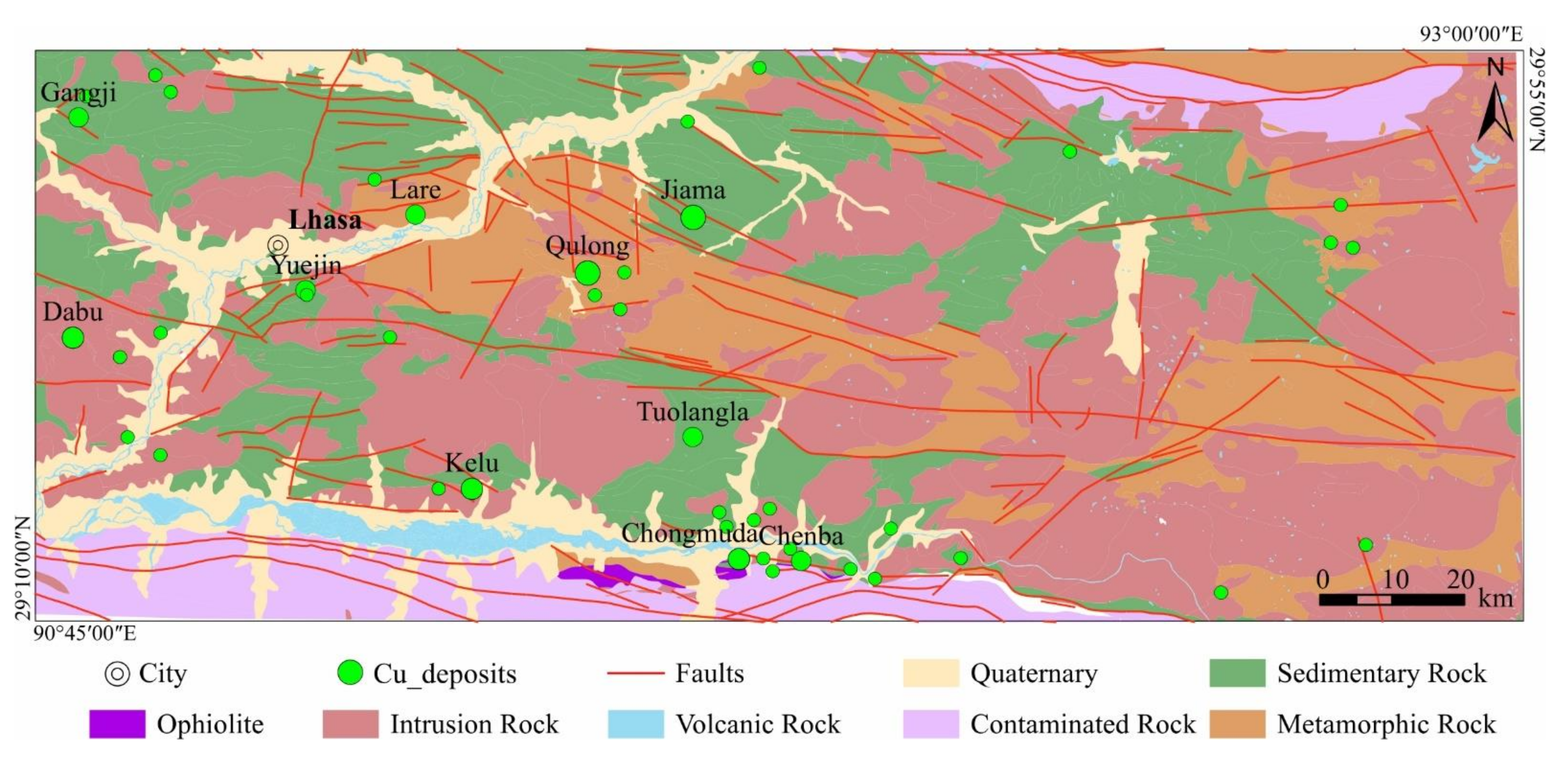
3.1. Geological Setting

The study area, the so-called ”Mila Mountain Integrated Exploration Region”, is located in the eastern Gangdese metallogenic belt in Tibet, southwest China (29°10′ N–29°55′ N; 90°45′ E–93°00′ E), with an area of about 12,290 km², which is one of the most famous copper mineralization areas in Tibet [39,40,41,42] (Figure 2). The subduction of the Neo-Tethyan Oceanic crust beneath the Asian plate from the Jurassic to the Cretaceous period and the subsequent collision of Indian–Asian plates in the Paleocene period and post-collisional magmatism in the Miocene period formed the specifically geological background and metallogenic conditions [43,44]. Mineralization is associated with the post-collisional small-volume intrusions, which intruded both pre- and syn-collisional granitic batholiths and the earlier stratigraphic volcano-sedimentary sequences [44,45,46,47,48]. Sedimentary rocks include clay stone, sandstone, shale, lithic sandstone, mudstone, and limestone from the Paleozoic to Cenozoic periods, and most of the outcrop sedimentary rocks are from the Cenozoic period. There have been intense intrusion activities in the past geological periods, especially in Mesozoic and Cenozoic. Intrusions that crop out at the surface in this area are mainly intermediate-acid intrusive rocks, and are controlled by the orientations of structures. The main faults have E–W, N–E, and N–S orientations. The fault systems control the mineralization and distribution of mineral deposits in the study area. The E–W-oriented faults control the distribution of copper deposits, and the faults with N–E and N–S orientations provide favorable conditions for Cu, Mo, Au, Pb, Zn, and other metal deposits [49] (Figure 2).

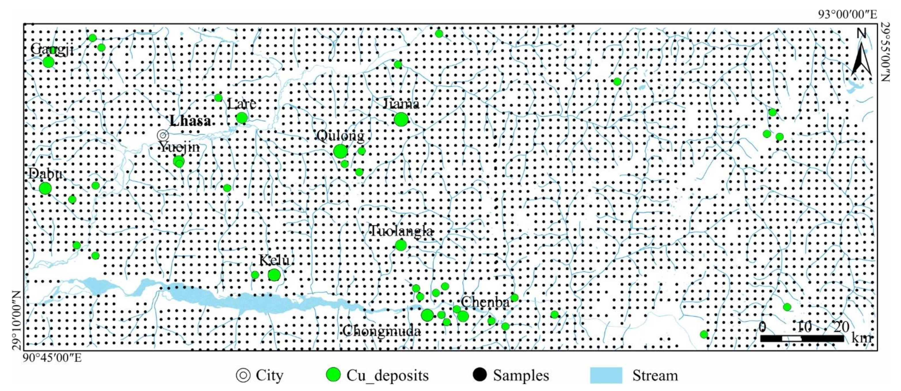
3.2. Geochemical Data

The geochemical dataset in this study is part of the “Regional Geochemistry National Reconnaissance (RGNR) Project”, which was initiated in 1979 and has covered more than 7 million km² of Chinese territory with stream sediment sampling and multi-element analysis of 39 elements (including Bi, Cu, P, La, Li, Ag, Sn, Au, Mo, Th, U, W, Sb, Hg, Mn, Cr, Sr, Nb, Pb, Ni, Ti, Y, Cd, Co, Ba, Be, V, Zn, B, As, Zr, F, Fe₂O₃, K₂O, CaO, MgO, Na₂O, Al₂O₃, and SiO₂) [50]. The sample density is 1 sample per 4 km², and a total of 4141 samples were collected in this research area (Figure 3). The 39 elements were analyzed by various methods (mainly including ICP-MS, XRF, and ICP-AES). The specific test methods, detection limits, quality control, and other information corresponding to each element can be found in the relevant literature [50,51].

4. Results and Discussions

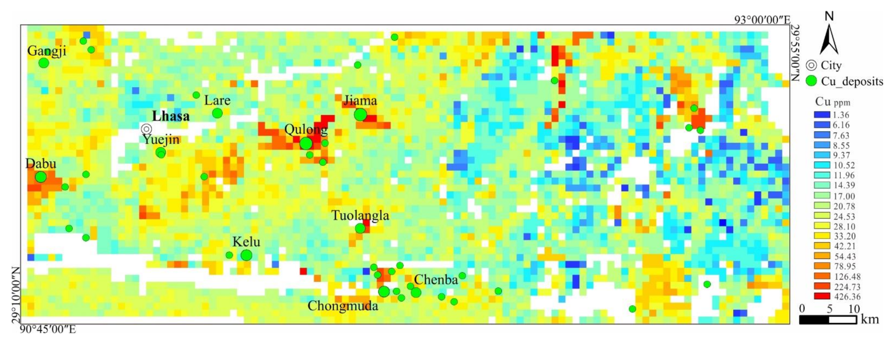
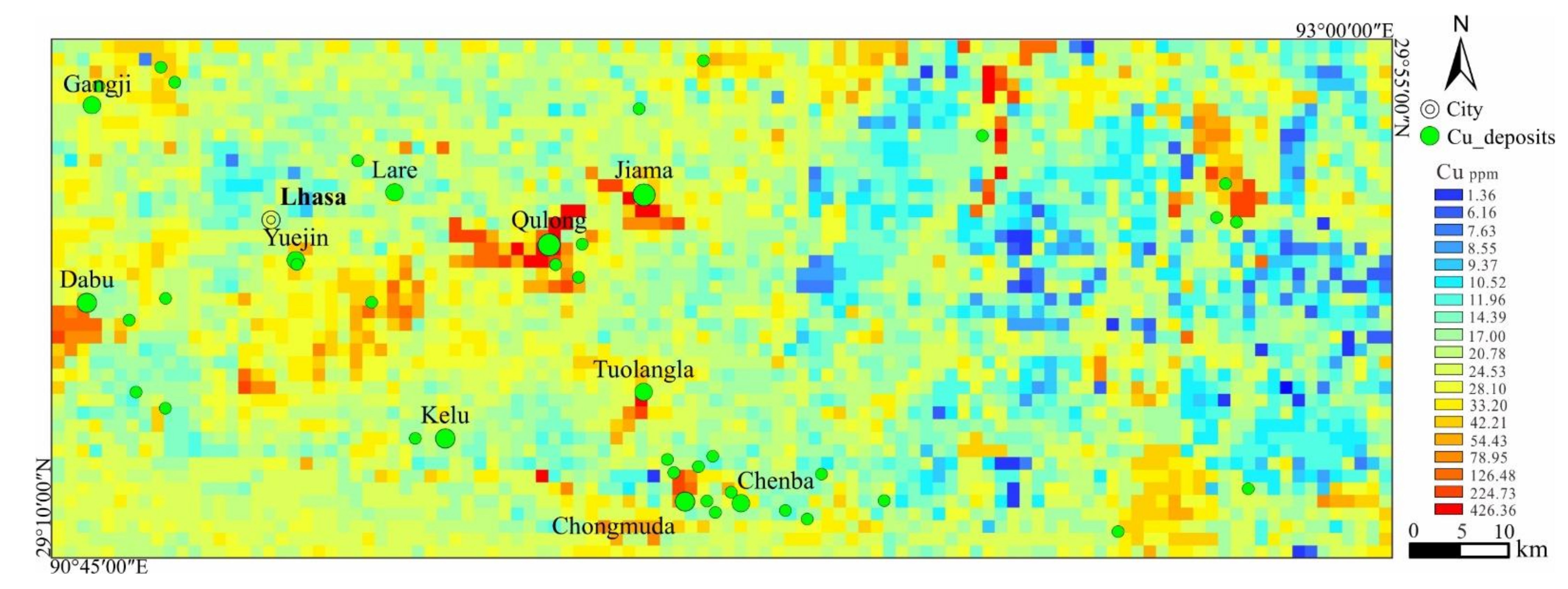
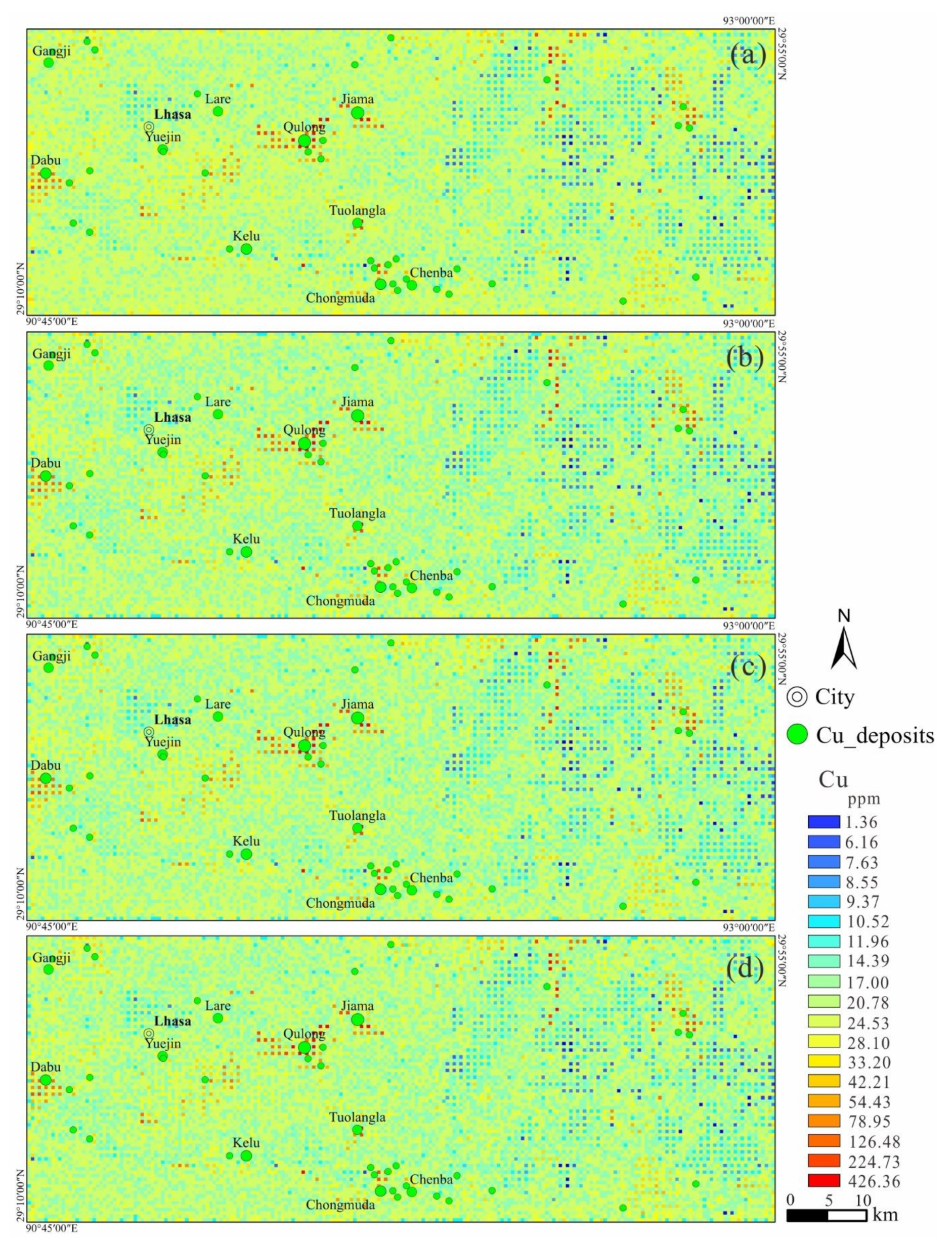
4.1. Direct Sampling Algorithm Simulation of Copper Element

Copper deposits are the most important potential mineral resource in this study area, and several significant copper deposits have been discovered, such as Qulong and Jiama. Therefore, the Cu element data were selected to verify the feasibility of multiple-point geostatistical simulation by evaluating the uncertainty of Cu anomalies and identifying the mineral resource prospective targets.

As mentioned above (Section 3.2), the geochemical data in the study area are from regular sampling (2 km × 2 km), and are sufficient to offer abundant multiple-point patterns. Therefore, less information would be lost when transferring such geochemical data into raster data.

The direct sampling algorithm was used to simulate the distribution of Cu. First, the original sample data of the Cu element were converted into raster data. The study area was divided into 108 × 41 grids with a grid size of 2 km × 2 km, according to the actual sampling interval, in order to minimize information loss (Figure 4). These raster data can not only be regarded as the grid that needs to be simulated, but can also be considered as the “training image” from which the multiple-point patterns required for the simulation are derived. The DS simulation of the raster data using the parameters set in

Table 2. DS parameters for the case study.

Parameter	Notation	Value
Number of realizations	L	200
Number of points in the data event	n	20
Max fraction of input data to scan	f	0.8
Distance threshold	t	0.02
Search radii	r	15
Path type		Fully random path

was performed, and the result is shown in Figure 5.

Subsequently, in order to obtain more detailed information, the study area was divided into 216 × 82 grids with a grid size of 1 km × 1 km, and then the original data were converted into raster data using this grid size (Figure 6), with Figure 5 as the training image and the raster data as conditional data. The Direct Sampling algorithm was used once again to simulate the value within the null value grid, generating 200 equal probability realizations [26,52].

Four out of 200 realizations generated by the Direct Sampling algorithm simulation were arbitrarily selected (Figure 7). It was found that the smoothing effect did not appear. As the original data and their statistical features were honored, the simulated realizations reflected the element concentration and even its spatial distribution patterns. The small discrepancies among these realizations are called ergodic fluctuations [13,14], and are to be expected, because the paths of each realization are different, and the values of the unsampled location are related to all the values in the vicinity; any position in the neighborhood where the value is uncertain may propagate its uncertainty, resulting in uncertainty of the realization.

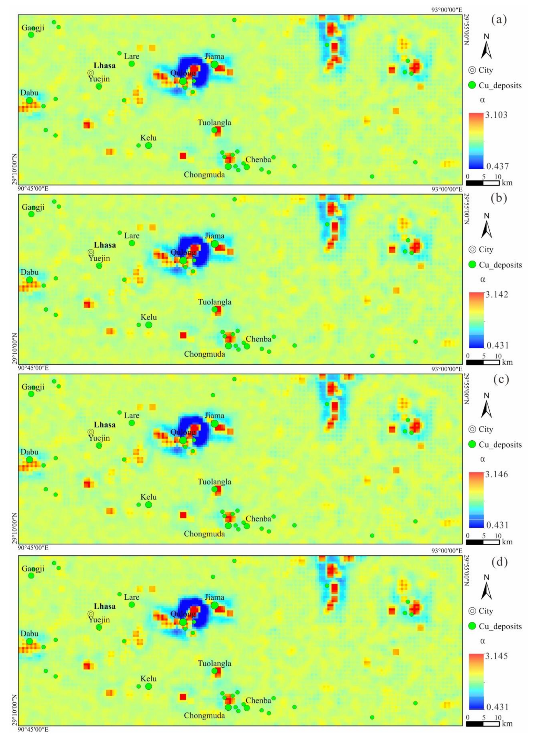
4.2. Stochastic Simulation-Based LSA

Local singularity analysis was used to process realizations from the DS algorithm. Square scanning windows with 3 × 3 km², 5 × 5 km², 7 × 7 km²…, 15 × 15 km² were adopted for this LSA (Figure 8).

All results of corresponding LSA associated with realizations can represent the uncertainty of local singularity, which is propagated from unsampled locations [53].

The E-type α method measures the mean value or trend of the singularity (Figure 9a). It can be seen that the E-type α map can better show the continuity of spatial distribution patterns. The E-type α variance can express the variety of the uncertainty where the maximum predicted variance means the maximum uncertainty, and vice versa (Figure 9b). The locations near the edge have a higher uncertainty, which may be caused by the limited values involved in the LSA estimation [14].

When comparing the results among simulation-based LSA (Figure 9a), kriging interpolation (Figure 10a), and kriging interpolation-based LSA (Figure 10b), a similar distribution of Cu is shown in macroscopy, but the smooth effect is clear in Figure 10. Comparatively speaking, as the original data were honored and the mean singularity was represented, the simulation-based LSA has a more powerful ability to reflect geochemical distribution patterns.

Delineating anomaly areas is one of the most important steps in geochemical mapping. Reasonable thresholds of certain elements are the key requirement. In this paper, the singularity-quantile (S-Q) analysis method was used to determine the geochemical anomaly thresholds: (1) the 99% confidence interval of E-type Cu singularity index was selected; (2) the normal reference line and residual fitting curve were determined through the 15th and 85th percentiles [41]. E-type singularity index values 1.943 and 2.059 were determined as the thresholds, which divided the spatial distribution patterns into three parts (Figure 11a). These two values can represent enrichment (α < 1.943) and depletion (α > 2.059), respectively (Figure 11b).

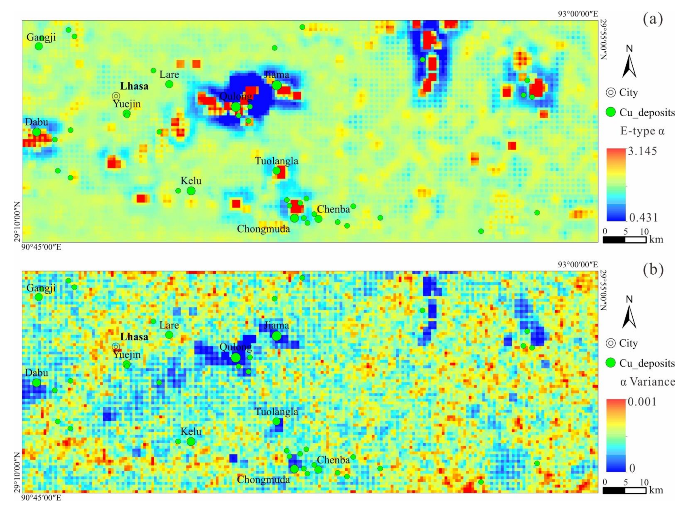
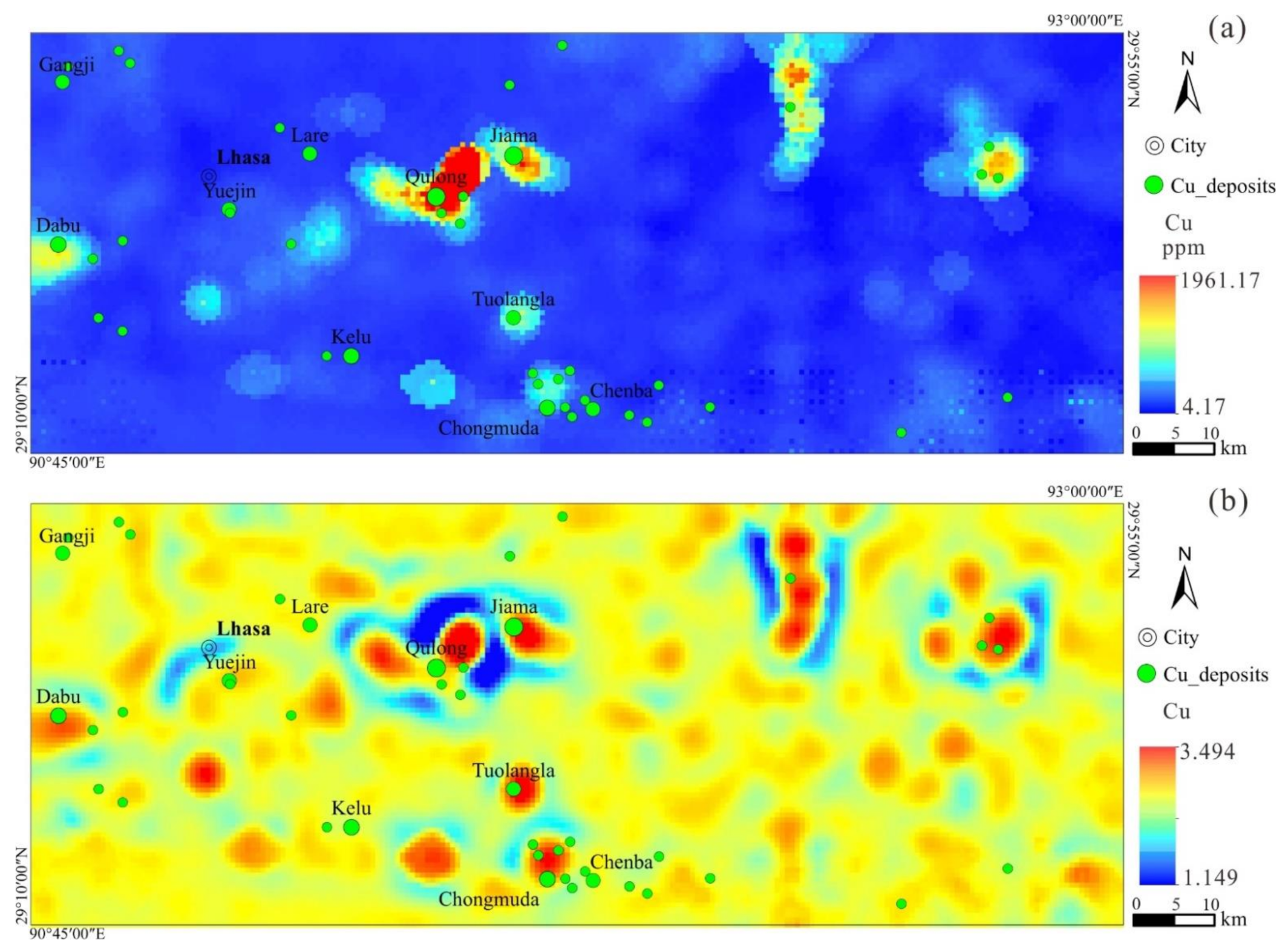
4.3. Uncertainty Assessment of Geochemical Anomaly

Uncertainty of the target attribute can be expressed as a probability map determined by a certain threshold [13,54]. Based on the singularity index map and the thresholds (α < 1.943) obtained in Section 4.2, the anomaly probability of Cu element can be calculated by the equation in Section 2.3. The anomaly probability map shows a close relationship between the high anomaly probability areas and known copper deposits (Figure 12). In fact, the high anomaly probability area always occurs on the edge of intermediate-acid intrusions or on the side of faults, which are the favorable metallogenic areas in this study region. Furthermore, combining the geological background and the favorable metallogenic conditions in the study area, such as intermediate-acid intrusions, intersection of faults, and favorable sedimentary rocks, several preliminary mineral prospective targets are proposed in Figure 13.

5. Conclusions

(1) In this paper, the direct sampling algorithm and local singularity analysis were used to delineate geochemical distribution patterns and evaluate the uncertainty of geochemical anomalies. Compared with deterministic methods (such as kriging), the methods effectively solve the problem of the smoothing effect and uncertainty of unsampled values.

(2) The anomaly uncertainty estimate of copper based on stream sediments data in the Mila Mountain Integrated Exploration Region of Tibet, China, is taken as an example to verify the feasibility of the methods. The multiple-point geostatistical simulation produced 200 equal-probability realizations, subsequently generated relative LSA maps, and then two separation thresholds of E-type α-value were calculated by the S-Q method, where α < 1.943 was obtained from the anomaly probability mapping. It can be seen from the probability map that the high anomaly probability areas are usually distributed near/on the fault or intrusions, and have a close correlation with the known deposits. According to the anomaly probability and geological conditions, some targets of interest have been preliminarily delineated, which should be focused on in subsequent mineral exploration.

References

1. Cheng, Q. Singularity theory and methods for mapping geochemical anomalies caused by buried sources and for predicting undiscovered mineral deposits in covered areas. J. Geochem. Explor. 2012, 122, 55–70. [Google Scholar] [CrossRef]
2. Xiong, Y.; Zuo, R.; Wang, K.; Wang, J. Identification of geochemical anomalies via local RX anomaly detector. J. Geochem. Explor. 2018, 189, 64–71. [Google Scholar] [CrossRef]
3. Matheron, G. Traité de Géostatistique Appliquée; Éditions Technip: Paris, France, 1962. [Google Scholar]
4. Huijbregts, C.J. Mining Geostatistics; Academic Press: Cambridge, MA, USA, 1978. [Google Scholar]
5. Bilonick, R.A. An introduction to applied geostatistics. Technometrics 1989, 33, 483–485. [Google Scholar] [CrossRef]
6. Shepard, D. A two-dimensional interpolation function for irregularly-spaced data. In Proceedings of the 1968 ACM National Conference, New York, NY, USA, 27–29 August 1968. [Google Scholar]
7. Tilke, C. Statistics for Spatial Data; John Wiley & Sons Inc.: Hoboken, NJ, USA, 1993. [Google Scholar]
8. Handcock, M.S.; Nychka, M.D. Kriging and splines: An empirical comparison of their predictive performance in some applications: Comment. J. Am. Stat. Assoc. 1994, 89, 401–403. [Google Scholar] [CrossRef]
9. Collins, F.C. A Comparison of Spatial Interpolation Techniques in Temperature Estimation; Virginia Polytechnic Institute and State University: Blacksburg, VA, USA, 1995. [Google Scholar]
10. Hartkamp, A.D.; De Beurs, K.; Stein, A.; White, J.W. Interpolation Techniques for Climate Variables Interpolation; International Maize and Wheat Improvement Center (CIMMYT): Mexico City, Mexico, 1999. [Google Scholar]
11. Stahl, K.; Moore, R.D.; Floyer, J.A.; Asplin, M.G.; Mckendry, I.G. Comparison of approaches for spatial interpolation of daily air temperature in a large region with complex topography and highly variable station density. Agric. For. Meteorol. 2006, 139, 224–236. [Google Scholar] [CrossRef]
12. Zuo, R. Exploring the effects of cell size in geochemical mapping. J. Geochem. Explor. 2012, 112, 357–367. [Google Scholar] [CrossRef]
13. Goovaerts, P. Geostatistical modelling of uncertainty in soil science. Geoderma 2001, 103, 3–26. [Google Scholar] [CrossRef]
14. Yue, L.; Qiuming, C.; Carranza, E.J.M.; Zhou, K. Assessment of geochemical anomaly uncertainty through geostatistical simulation and singularity analysis. Nat. Resour. Res. 2018, 28, 199–212. [Google Scholar]
15. Mery, N.; Emery, X.; Cáceres, A.; Ribeiro, D.; Cunha, E. Geostatistical modeling of the geological uncertainty in an iron ore deposit. Ore Geol. Rev. 2017, 88, 336–351. [Google Scholar] [CrossRef]
16. Qu, J.; Deutsch, C.V. Geostatistical simulation with a trend using gaussian mixture models. Nat. Resour. Res. 2017, 27, 347–363. [Google Scholar] [CrossRef]
17. Paithankar, A.; Chatterjee, S. Grade and tonnage uncertainty analysis of an African copper deposit using multiple-point geostatistics and sequential gaussian simulation. Nat. Resour. Res. 2017, 27, 419–436. [Google Scholar] [CrossRef]
18. Hosseini, S.A.; Asghari, O. Multivariate geostatistical simulation on block-support in the presence of complex multivariate relationships: Iron ore deposit case study. Nat. Resour. Res. 2018, 28, 125–144. [Google Scholar] [CrossRef]
19. Rahimi, H.; Asghari, O.; Hajizadeh, F. Selection of optimal thresholds for estimation and simulation based on indicator values of highly skewed distributions of ore data. Nat. Resour. Res. 2018, 27, 437–453. [Google Scholar] [CrossRef]
20. Guardiano, F.B.; Srivastava, R.M. Multivariate geostatistics: Beyond bivariate moments. In Geostatistics Troia ’92; Kluwer: Dordrecht, The Netherlands, 1993; Volume 1, pp. 133–144. [Google Scholar]
21. Bezrukov, A.; Davletova, A.R. Methods of multiplepoint statistics in geological simulation practice: Prospects for application. In Proceedings of the SPE Russian Oil and Gas Conference and Exhibition, Moscow, Russia, 26–28 October 2010. (In Russian). [Google Scholar]
22. Parra, Á.; Ortiz, J.M. Adapting a texture synthesis algorithm for conditional multiple point geostatistical simulation. Stoch. Environ. Res. Risk Assess. 2011, 25, 1101–1111. [Google Scholar] [CrossRef]
23. Mahmud, K.; Mariethoz, G.; Caers, J.; Tahmasebi, P.; Baker, A. Simulation of Earth textures by conditional image quilting. Water Resour. Res. 2014, 50, 3088–3107. [Google Scholar] [CrossRef] [Green Version]
24. Abdollahifard, M.J. Fast multiple-point simulation using a data-driven path and an efficient gradient-based search. Comput. Geosci. 2016, 86, 64–74. [Google Scholar] [CrossRef]
25. Strebelle, S. Conditional simulation of complex geological structures using multiple-point statistics. Math. Geol. 2002, 34, 1–21. [Google Scholar] [CrossRef]
26. Mariethoz, G.; Renard, P.; Straubhaar, J. The direct sampling method to perform multiple-point geostatistical simulations. Water Resour. Res. 2010, 46, W11536. [Google Scholar] [CrossRef] [Green Version]
27. Chen, Q.; Mariethoz, G.; Liu, G.; Comunian, A.; Ma, X. Locality-based 3-D multiple-point statistics reconstruction using 2-D geological cross sections. Hydrol. Earth Syst. Sci. 2018, 22, 6547–6566. [Google Scholar] [CrossRef] [Green Version]
28. Arpat, G.B.; Caers, J. Conditional simulation with patterns. Math. Geol. 2007, 39, 177–203. [Google Scholar] [CrossRef]
29. Zhang, T.; Switzer, P.; Journel, A. Filter-Based classification of training image patterns for spatial simulation. Math. Geol. 2006, 38, 63–80. [Google Scholar] [CrossRef]
30. Tahmasebi, P.; Hezarkhani, A.; Sahimi, M. Multiple-Point geostatistical modeling based on the cross-correlation functions. Comput. Geosci. 2012, 16, 779–797. [Google Scholar] [CrossRef]
31. Bohling, G.C. Petroleum Geostatistics; Jef Caers Society of Petroleum Engineers: Richardson, TX, USA, 2005; p. 96. ISBN 978-1-55563-106-2. [Google Scholar]
32. Mariethoz, G.; Caers, J. Multiple-Point Geostatistics: Stochastic Modeling with Training Images; Wiley-Blackwell: Hoboken, NJ, USA, 2014. [Google Scholar]
33. Yang, L.; Hou, W.; Cui, C.; Cui, J. GOSIM: A multi-scale iterative multiple-point statistics algorithm with global optimization. Comput. Geosci. 2016, 89, 57–70. [Google Scholar] [CrossRef]
34. Sadeghi, B.; Madani, N.; Carranza, E.J.M. Combination of geostatistical simulation and fractal modeling for mineral resource classification. J. Geochem. Explor. 2015, 149, 59–73. [Google Scholar] [CrossRef]
35. Dagasan, Y.; Renard, P.; Straubhaar, J.; Erten, O.; Topal, E. Automatic parameter tuning of multiple-point statistical simulations for lateritic bauxite deposits. Minerals 2018, 8, 220. [Google Scholar] [CrossRef] [Green Version]
36. Cheng, Q. Mapping singularities with stream sediment geochemical data for prediction of undiscovered mineral deposits in Gejiu, Yunnan Province, China. Ore Geol. Rev. 2007, 32, 314–324. [Google Scholar] [CrossRef]
37. Cheng, Q.; Agterberg, F.P. Singularity analysis of ore-mineral and toxic trace elements in stream sediments. Comput. Geosci. 2009, 35, 234–244. [Google Scholar] [CrossRef]
38. Liu, Y.; Zhou, K.; Cheng, Q. A new method for geochemical anomaly separation based on the distribution patterns of singularity indices. Comput. Geosci. 2017, 105, 139–147. [Google Scholar] [CrossRef]
39. Lin, B.; Chen, Y.; Tang, J.; Wang, Q.; Song, Y.; Yang, C.; Wang, W.; He, W.; Zhang, L. 40Ar/39Ar and Rb-Sr ages of the tiegelongnan porphyry Cu-(Au) deposit in the Bangong Co-Nujiang metallogenic belt of Tibet, China: Implication for generation of super-large deposit. Acta Geol. Sin. (Engl. Ed.) 2017, 91, 602–616. [Google Scholar] [CrossRef]
40. Lin, B.; Tang, J.X.; Chen, Y.C.; Song, Y.; Hall, G.; Wang, Q.; Yang, C.; Fang, X.; Duan, J.-L.; Yang, H.-H.; et al. Geochronology and genesis of the tiegelongnan porphyry Cu(Au) deposit in Tibet: Evidence from U–Pb, Re–Os dating and Hf, S, and H–O isotopes. Resour. Geol. 2017, 67, 1–21. [Google Scholar] [CrossRef] [Green Version]
41. Song, Y.; Yang, C.; Wei, S.; Yang, H.; Fang, X.; Lu, H. Tectonic control, reconstruction and preservation of the Tiegelongnan porphyry and epithermal overprinting Cu (Au) deposit, central Tibet, China. Minerals 2018, 8, 398. [Google Scholar] [CrossRef] [Green Version]
42. Lin, B.; Tang, J.; Chen, Y.; Baker, M.; Song, Y.; Yang, H.; Wang, Q.; He, W.; Liu, Z. Geology and geochronology of Naruo large porphyry-breccia Cu deposit in the Duolong district, Tibet. Gondwana Res. 2018, 66, 168–182. [Google Scholar] [CrossRef]
43. Hou, Z.; Yang, Z.; Qu, X.; Meng, X.; Li, Z.; Beaudoin, G.; Rui, Z.; Gao, Y.; Zaw, K. The miocene gangdese porphyry copper belt generated during post-collisional extension in the Tibetan Orogen. Ore Geol. Rev. 2009, 36, 25–51. [Google Scholar] [CrossRef]
44. Turner, S.; Hawkesworth, C.; Liu, J.; Rogers, N.; Kelley, S.; van Calsteren, P. Timing of Tibetan uplift constrained by analysis of volcanic rocks. Nature 1993, 364, 50. [Google Scholar] [CrossRef]
45. Miller, C.H.; Schuster, R.; Klötzli, U.; Frank, W.; Purtscheller, F. Post-Collisional potassic and ultrapotassic magmatism in SW Tibet: Geochemical and Sr–Nd–Pb–O isotopic constraints for mantle source characteristics and petrogenesis. J. Petrol. 1999, 40, 1399–1424. [Google Scholar] [CrossRef]
46. Chung, S.-L.; Liu, D.; Ji, J.; Chu, M.-F.; Lee, H.-Y.; Wen, D.-Y.; Lo, C.-H.; Lee, T.-Y.; Qian, Q.; Zhang, Q. Adakites from continental collision zones: Melting of thickened lower crust beneath southern Tibet. Geology 2003, 31, 1021–1024. [Google Scholar] [CrossRef] [Green Version]
47. Pan, G.-T. Spatial temporal framework of the Gangdese Orogenic Belt and its evolution. Acta Petrol. Sin. 2006, 22, 521–533. [Google Scholar]
48. Xiao, K.; Li, N.; Porwal, A.; Holden, E.-Y.; Bagas, L.; Lu, Y. GIS-Based 3D prospectivity mapping: A case study of Jiama copper-polymetallic deposit in Tibet, China. Ore Geol. Rev. 2015, 71, 611–632. [Google Scholar] [CrossRef]
49. Zuo, R.; Cheng, Q.; Agterberg, F.P.; Xia, Q. Application of singularity mapping technique to identify local anomalies using stream sediment geochemical data, a case study from Gangdese, Tibet, western China. J. Geochem. Explor. 2009, 101, 225–235. [Google Scholar] [CrossRef]
50. Xie, X. Analytical requirements in international geochemical mapping. In Analyst; London Society of Public Analysts, Royal Society of Chemistry: London, UK, 1995. [Google Scholar]
51. Wang, X. Exploration geochemistry: Past achievements and future challenges. Earth Sci. Front. 2003, 10, 239–248. [Google Scholar]
52. Wang, J.; Zuo, R. Identification of geochemical anomalies through combined sequential Gaussian simulation and grid-based local singularity analysis. Comput. Geosci. 2018, 118, 52–64. [Google Scholar] [CrossRef]
53. Wang, J.; Zuo, R. Recognizing geochemical anomalies via stochastic simulation-based local singularity analysis. J. Geochem. Explor. 2019, 198, 29–40. [Google Scholar] [CrossRef]
54. Goovaerts, P. Geostatistics for natural resources evaluation (Applied geostatistics). In Geostatistics for Natural Resources Evaluation; Oxford University Press: Oxford, UK, 1997. [Google Scholar]
Figure 1. Simulation path of the dynamic organization.
Minerals 11 01037 g001
Figure 2. Simplified geological map of the study area.
Minerals 11 01037 g002
Figure 3. Geochemical sample locations.
Minerals 11 01037 g003
Figure 4. Raster map of Cu: the study area is divided into 108 × 41 grids with a grid size of 2 km × 2 km.
Minerals 11 01037 g004
Figure 5. The realization of Cu: the study area is divided into 108 × 41 grids with a grid size of 2 km × 2 km.
Minerals 11 01037 g005
Figure 6. Raster map of Cu: the study area is divided into 216 × 82 grids with a grid size of 1 km × 1 km.
Minerals 11 01037 g006
Figure 7. A random sample of 4 out of 200 realizations generated by direct simulation: (a) realization #15, (b) realization #58, (c) realization #130, and (d) realization #186.
Minerals 11 01037 g007
Figure 8. Corresponding local singularity analysis results of the four realizations: (a) LSA #15, (b) LSA #58, (c) LSA #130, and (d) LSA #186.
Minerals 11 01037 g008
Figure 9. (a) The E-type α map and (b) the α variance map.
Minerals 11 01037 g009
Figure 10. (a) The distribution of Cu by ordinary kriging and (b) the kriging interpolation-based LSA.
Minerals 11 01037 g010
Figure 11. E-type α map by means of S-Q method in (a) frequency domain and (b) spatial domain.
Minerals 11 01037 g011
Figure 12. Probability maps of geochemical anomaly with α < 1.943.
Minerals 11 01037 g012
Figure 13. Prospective targets of mineral resources.
Minerals 11 01037 g013