Reactive Transport Modelling of the Long-Term Interaction between Carbon Steel and MX-80 Bentonite at 25 °C

Abstract

The geological disposal in deep bedrock repositories is the preferred option for the management of high-level radioactive waste (HLW). In some of these concepts, carbon steel is considered as a potential canister material and bentonites are planned as backfill material to protect metallic waste containers. Therefore, a 1D radial reactive transport model has been developed in order to better understand the processes occurring during the long-term iron-bentonite interaction. The numerical model accounts for diffusion, aqueous complexation reactions, mineral dissolution/precipitation and cation exchange at a constant temperature of 25$°\mathrm{C}$ under anoxic conditions. Our results suggest that Fe is sorbed at the montmorillonite surface via cation exchange in the short-term, and it is consumed by formation of the secondary phases in the long-term. The numerical model predicts precipitation of nontronite, magnetite and greenalite as corrosion products. Calcite precipitates due to cation exchange in the short-term and due to montmorillonite dissolution in the long-term. Results further reveal a significant increase in pH in the long-term, while dissolution/precipitation reactions result in limited variations of the porosity. A sensitivity analysis has also been performed to test the effect of selected parameters, such as corrosion rate, diffusion coefficient and composition of the bentonite porewater, on the corrosion processes. Overall, outcomes suggest that the predicted main corrosion products in the long-term are Fe-silicate minerals, such phases thus should deserve further attention as a chemical barrier in the diffusion of radionuclides to the repository far field.

1. Introduction

Burial in a stable deep geological formation is the generally accepted strategy for the safe management of high-level radioactive waste. In some repository concepts, the waste is foreseen to be emplaced in metallic canisters (e.g., made of carbon steel), which would be surrounded by bentonite as buffer material (engineered barrier system or EBS). During the geochemical evolution of such a repository system, groundwater is expected to move through the barriers and contact the metallic canisters, which will start corroding. In case of canister failure and subsequent waste matrix alteration, bentonite, consisting mainly of montmorillonite, would be able to retain the released radionuclides. However, during container corrosion, long-term geochemical processes at the corroding container/bentonite interface will proceed and have an impact on the properties of the geotechnical barrier. Such information may be of relevance for the Safety Case of the repository. To gain insights into container corrosion and bentonite alteration, several experiments and numerical models studying the iron-bentonite interactions have been reported in literature (see, e.g., in [1,2,3,4,5]).

In laboratory experiments at 90$°\mathrm{C}$ studying the interaction between iron and argillite [6,7], or iron and bentonite [8], the formation of a layer of secondary phases, made of magnetite, siderite and Fe-silicates such as nontronite and cronstedtite, was found at the reacting interface. More recently, Kaufhold et al. [9] reported that the presence of highly reactive silica results in the predominant formation of Fe-silicates as corrosion products rather than magnetite. These findings suggest that the nature of formed corrosion products depends on the composition of the infiltrating porewater and thus on the mineralogical composition of the bentonite and argillite but also on the coupling of reaction kinetics and transport. Some of these reactions take a long time and cannot be reproduced over laboratory time scales [10]. Due to the strong coupling of kinetically controlled dissolution/precipitation/transport processes, reactive transport models play an important role for studying the long-term iron-bentonite interaction. Some of the reactive transport calculations considered magnetite and siderite as principal corrosion products [11,12], and most of them also considered the formation of Fe-silicates such as berthierine, greenalite or cronstedtite [10,13,14,15,16,17,18,19]. The predicted results suggested that not only magnetite but also Fe-silicates can form during the long-term iron-bentonite interaction. Hence, the conceptual model considered has an effect on the predicted results. For instance, some reported reactive transport models considered a gap between the canister and the bentonite (see, e.g., in [15,18]), but this approach enhances the alteration of both canister and bentonite because the reactive surface area is much larger than the one considering that canister and bentonite are in contact without any gap in between. In the real system, any gap would be closed due to bentonite swelling upon hydration. Thus, the reactive surface area of the bentonite minerals is only related to the porosity of the bentonite. Other authors considered the canister as porous material (see, e.g., in [13,19]) allowing dissolution of the canister and precipitation of corrosion products within the canister pores. However, in the real system, the canister can only react at the interface with bentonite due to the presence of porewater. The temperature of the system is under discussion in the literature, some reported reactive transport models of EBS in clays considered a fully water-saturated isothermal system with a temperature of 50$°\mathrm{C}$ [13], 70$°\mathrm{C}$ [18] or 100$°\mathrm{C}$ [17,20] conditioning the nature of the secondary phases that can form during the long-term interaction. However, according to Finsterle et al. [21], the heat pulse could last between a few decades to a few hundred years, then the ambient temperature prior to waste emplacement will prevail in the long-term anaerobic conditions. Then, a temperature around 25$°\mathrm{C}$ would be expected from the depth taking into account the geothermal gradient. Indeed, isothermal reactive transport models at 25$°\mathrm{C}$ have been reported [19], however, for an EBS in granite.

The objective of this study is, therefore, to better understand the processes that will occur in the long-term iron-bentonite (i.e., MX-80) interaction and the nature of the secondary phases for an EBS in clay rock by means of reactive transport models. The conceptual model assumes that bentonite is fully water-saturated and that heat pulse is already dissipated, therefore, anaerobic conditions at a constant temperature of 25$°\mathrm{C}$ are considered. Reported corrosion products that were found experimentally [6,8,22,23] are considered as potential secondary phases. Due to the lack of long-term experimental data, our results are compared with other published numerical studies on iron–clay/bentonite interaction [13,18,19]. The conceptual model and the results of the reference model are presented in Section 2 and Section 3 respectively. In addition, a sensitivity analysis, Section 4, has been performed in order to study the effect of selected parameters, such as corrosion rate, diffusion coefficient, reactive surface area and the porewater composition, on the corrosion products.

2. Reactive Transport Model

2.1. Processes and Governing Equations

The simulations were carried out using Retraso-CodeBright [24]. This software package couples CodeBright [25], a finite element computer code that can handle multiphase flow and heat transfer to a module for reactive transport, which includes aqueous complexation reactions, precipitation/dissolution of minerals and adsorption. For more details about the code we refer to Olivella et al. [25] and Saaltink et al. [24]. Only an outline of the main processes taken into account in the present work is given here.

The conceptual model considers that the system is fully water-saturated, then the mass balance of reactive transport can be written as

$${\mathbf{U}}_{\mathbf{a}}\frac{\delta \varphi {\rho }_{\mathrm{l}}{\mathbf{c}}_{\mathbf{a}}}{\delta t}+{\mathbf{U}}_{\mathbf{d}}\frac{\delta \varphi {\rho }_{\mathrm{l}}{\mathbf{c}}_{\mathbf{d}}}{\delta t}+{\mathbf{U}}_{\mathbf{m}}\frac{\delta (1-\varphi ){\rho }_{\mathrm{s}}{\mathbf{c}}_{\mathbf{m}}}{\delta t}={\mathbf{U}}_{\mathbf{a}}i\left({\mathbf{c}}_{\mathbf{a}}\right)+\mathbf{U}{\mathbf{S}}_{\mathbf{k}}^{\mathbf{t}}{\mathbf{r}}_{\mathbf{m}}\left({\mathbf{c}}_{\mathbf{a}}\right)$$

(1)

where $\varphi$ is the porosity, ${\rho }_{\mathrm{l}}$ and ${\rho }_{\mathrm{s}}$ are the liquid and solid densities, respectively (kg ${\mathrm{m}}^{-3}$). Vectors ${\mathbf{c}}_{\mathbf{a}}$, ${\mathbf{c}}_{\mathbf{d}}$ and ${\mathbf{c}}_{\mathbf{m}}$ (mol ${\mathrm{kg}}^{-1}$) are the concentrations of aqueous species, adsorbed species and minerals respectively. Matrix ${\mathbf{S}}_{\mathbf{k}}^{\mathbf{t}}$ and vector ${\mathbf{r}}_{\mathbf{m}}$ contain the stoichiometric coefficients and the rates of the kinetic reactions, which can be considered as functions of all aqueous concentrations. Matrices ${\mathbf{U}}_{\mathbf{a}}$, ${\mathbf{U}}_{\mathbf{d}}$ and ${\mathbf{U}}_{\mathbf{m}}$ are called the component matrices for aqueous, adsorbed and mineral species and relate the concentrations of the species with the total concentrations of the components. The matrix $\mathbf{U}$ is the component matrix for all species. These matrices can be computed from the stoichiometric coefficient of the chemical reactions. i is the diffusion term, and according to Fick’s law [25] can be written as

$$i\left({\mathbf{c}}_{\mathbf{a}}\right)=\nabla ·\left({\mathbf{D}}_{\mathbf{p}}\varphi {\rho }_{\mathrm{l}}\nabla \left({\mathbf{c}}_{\mathbf{a}}\right)\right)$$

(2)

where ${\mathbf{D}}_{\mathbf{p}}$ is the molecular diffusion coefficient in porous media (${\mathrm{m}}^2$ ${\mathrm{s}}^{-1}$):

$$D_p=\tau 1.1\times {10}^{-4}exp\left(\frac{-24530}{R(273.15+T)}\right)$$

(3)

$$D_e=\varphi D_p$$

(4)

where $\tau$ is the tortuosity factor, R = 8.31 J ${\mathrm{mol}}^{-1}$ ${\mathrm{K}}^{-1}$, T is the temperature (°C) and $D_e$ is the effective diffusion coefficient (${\mathrm{m}}^2$ ${\mathrm{s}}^{-1}$).

2.2. Conceptual Model

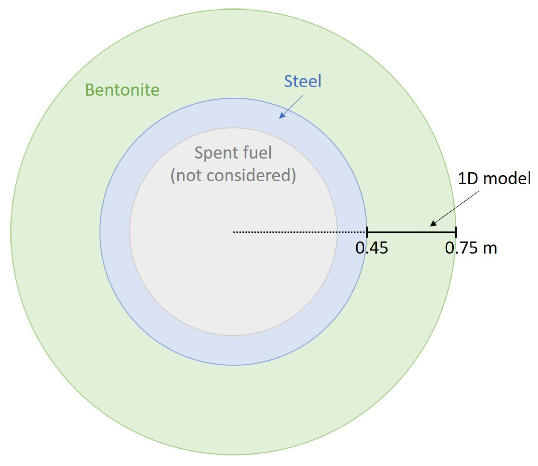
Our conceptual model considers a cylindrical carbon steel canister surrounded by bentonite (Figure 1). It takes into account the reactions that could occur during the interaction between steel, bentonite and the porewater. We assume anaerobic conditions, when the bentonite is fully water-saturated, and therefore interaction between canister, bentonite and porewater can occur. This also implies that the thermal pulse has dissipated [19,26], thus a temperature of 25$°\mathrm{C}$ is considered. No gas phase has been considered in the numerical model due to a water-saturated system, and the negligible presence of some type of dissolved gases such as hydrogen or ${\mathrm{CO}}_2$. These assumptions are similar to that reported in literature by other authors (see, e.g., in [19]) implying that the model does not consider the potential impact of ${\mathrm{H}}_2$ evolution on the integrity of the bentonite barrier. However, in the real system aerobic conditions will prevail first and temperature will decrease with time, and during the hydration process the bentonite will be altered. According to Bossart et al. [26], consumption of oxygen in bentonite pores will be consumed within decades. During this phase, a mixture of crystalline and amorphous Fe(II) and Fe(III) corrosion products will be generated [22]. Thermal equilibration usually is assumed to take decades up to some hundreds of years [26]. Recent simulations [27], however, result in much longer thermal equilibration times. This will have a certain influence on corrosion and alteration kinetics. However, the temperature dependence of iron corrosion rates appears to be moderate (see, e.g., in [28]). Full bentonite saturation is established after some decades [26,27,29]. As long as the packing density of the bentonite does not reach threshold values of 1250–1450 kg ${\mathrm{m}}^{-3}$ [30] significant microbial impact cannot be excluded. In experimental studies complex corrosion product mixtures are found, predominantly magnetite [30] but also sulphide minerals such a pyrite [31]. However, the anoxic steel corrosion phase under saturated bentonite conditions and at relatively low temperature appears to dominate thereafter for thousands of years. The main fraction of secondary iron corrosion phases will, thus, form under those conditions investigated in the present study and finally will represent the corrosion phase layer which will interact with radionuclides released from waste forms first upon loss of container integrity.

The geometry of the 1D axisymmetric model reflects the canister–bentonite interface and 0.3 m of bentonite (Figure 1). The canister is considered only as a node in the boundary. The bentonite is discretised into 45 unidimensional finite elements with sizes ranging from 0.5 cm near to the interface to 1 cm near to the boundary. The total iron–bentonite interaction time is 10,000 years. The model considers only diffusion as transport mechanism (Equation (2)). We assume a pore diffusion coefficient of 1 $\times {10}^{-10}$ ${\mathrm{m}}^2$ ${\mathrm{s}}^{-1}$ (Equation (3)) [19]. The porosity of bentonite is 0.4 [18,19], yielding an effective diffusion coefficient of 4 $\times {10}^{-11}$ ${\mathrm{m}}^2$ ${\mathrm{s}}^{-1}$ (Equation (4)).

Table 1. Comparison of the main differences in conceptual models between the present study and other reported models in the literature.

	Present Study	Bildstein et al. [13]	Wilson et al. [18]	Samper et al. [19]
Geometry	Canister as boundary	Porous canister	Canister as boundary and porous canister	Porous canister
Temperature	25$°\mathrm{C}$	50$°\mathrm{C}$	70$°\mathrm{C}$	25$°\mathrm{C}$
Bentonite	MX-80	MX-80	MX-80	FEBEX
Secondaryphases	Magnetite, nontronite greenalite, siderite cronstedtite	Magnetite, siderite, chamosite, saponite cronstedtite	Magnetite, siderite amesite, berthierine chlorite, greenalite, lizardite, analcime, cronstedtite, saponite	Magnetite, siderite analcime, cronstedtite
Corrosion rate	2 $\mathsf{\mu }$m ${\mathrm{y}}^{-1}$	4.3 $\mathsf{\mu }$m ${\mathrm{y}}^{-1}$	1 $\mathsf{\mu }$m ${\mathrm{y}}^{-1}$	2 $\mathsf{\mu }$m ${\mathrm{y}}^{-1}$
Interaction time	10,000 y	16,250 y	10,000 y	1 $\times {10}^6$ y

summarises our conceptual model, which is also compared with other reported numerical models.

2.3. Geochemical System

The geochemical model accounts for steel corrosion, aqueous complexation reactions, mineral dissolution/precipitation and cation exchange reactions.

2.3.1. Solid Composition

The mineral composition of MX-80 bentonite and the volumetric fractions of each mineral were based on that given by Karnland [32], which is comparable to the characterisation made by Kiviranta et al. [33]. The primary phases considered are montmorillonite, quartz, muscovite, albite, illite, pyrite and calcite. The volumetric fractions of each phase are listed in

Table 2. Bentonite mineralogical composition considered in the numerical model. The volumetric fractions are also listed for each phase.

Mineral	Volumetric Fraction (${\mathbf{m}}^3$${\mathbf{m}}^{-3}$)
Montmorillonite	5.01 $\times {10}^{-1}$
Quartz	4.70 $\times {10}^{-2}$
Albite	2.10 $\times {10}^{-2}$
Muscovite	2.10 $\times {10}^{-2}$
Illite	5.00 $\times {10}^{-3}$
Pyrite	4.00 $\times {10}^{-3}$
Calcite	1.00 $\times {10}^{-3}$

. We assume that carbon steel is composed only of iron, Fe(s), which is the main phase of carbon steel. The potential corrosion products considered in the numerical model have been selected according to published experiments [6,7,8,23] and from the Iron Corrosion in Bentonite (IC-A) experiment in the Mont-Terri rock laboratory (Switzerland) [22,31,34], which are magnetite, greenalite, cronstedtite, siderite, nontronite-Na and nontronite-Mg. Other modelling works reported in literature (see, e.g., in [18,19]) considered zeolites as secondary phases such as analcime; however, we did not consider them because they were not reported by Morelová et al. [31].

2.3.2. Solution Composition

Table 3. MX-80 bentonite initial porewater composition used in the numerical model. Imposed constraints to calculate some of these values (equilibrium with solids and charge balance) are also indicated.

Component	Water Composition (mol ${\mathbf{L}}^{-1}$)
${\mathrm{Al}\left(\mathrm{OH}\right)}_4^{-}$	2.00 $\times {10}^{-7}$
${\mathrm{Ca}}^{2+}$	8.60 $\times {10}^{-3}$
${\mathrm{Cl}}^{-}$	3.54 $\times {10}^{-2}$ charge balance
${\mathrm{Fe}}^{+2}$	7.19 $\times {10}^{-8}$
${\mathrm{HCO}}_3^{-}$	1.31 $\times {10}^{-3}$ calcite
${\mathrm{K}}^{+}$	2.50 $\times {10}^{-3}$
${\mathrm{Mg}}^{2+}$	6.50 $\times {10}^{-3}$
${\mathrm{Na}}^{+}$	7.30 $\times {10}^{-3}$
${\mathrm{SiO}}_2$(aq)	1.00 $\times {10}^{-4}$
${\mathrm{SO}}_4^{2-}$	1.70 $\times {10}^{-3}$
${\mathrm{O}}_2$(aq)	1.00 $\times {10}^{-15}$
pH	7.30

shows the chemical composition of the MX-80 bentonite initial porewater used in the numerical model. In the real system, the bentonite will be hydrated by the clay groundwater reacted with the concrete liner. Therefore, the composition of the MX-80 bentonite porewater will depend not only on the reactions with the primary phases of the materials, but also on the secondary phases formed during these reactions. In order to simplify the problem, the majority of authors in literature calculate the porewater as a result of the equilibrium of bentonite with a groundwater (see, e.g., in [35]). Other authors calculate the initial water composition of the bentonite using mineral constraints (see, e.g., in [13]). In this work, a clay groundwater that was not oversaturated with the minerals used in the model has been selected. The initial porewater calculated, first using PhreeqC, corresponds to the composition of the porewater used by Martin et al. [8,36] equilibrated with montmorillonite, because it is the main phase of the bentonite. Ca, Na, K, Fe, Mg, Al and Si are thus at equilibrium with the montmorillonite used in the numerical model (

Table 4. Equilibrium constants (log ${\mathrm{K}}_{eq}$ at 25$°\mathrm{C}$) of the minerals taken into account in the numerical model. Reactions are written as the dissolution of 1 mol of mineral in terms of the primary species ${\mathrm{Ca}}^{2+}$, ${\mathrm{Fe}}^{2+}$, ${\mathrm{SiO}}_2$(aq), ${\mathrm{Al}\left(\mathrm{OH}\right)}_4^{-}$, ${\mathrm{H}}^{+}$, ${\mathrm{SO}}_4^{2-}$, ${\mathrm{HCO}}_3^{-}$, ${\mathrm{K}}^{+}$, ${\mathrm{Na}}^{+}$, ${\mathrm{Mg}}^{2+}$, ${\mathrm{Cl}}^{-}$ and ${\mathrm{O}}_2$(aq).

Mineral	Formula/Reaction	log ${\mathbf{K}}_{\mathit{e}\mathit{q}}$
Iron	Fe(s) + 2${\mathrm{H}}^{+}$ + 0.5${\mathrm{O}}_2$(aq) = ${\mathrm{Fe}}^{2+}$ + ${\mathrm{H}}_2$O	59.01
Montmorillonite	${\mathrm{Ca}}_{0.02}$${\mathrm{Na}}_{0.15}$${\mathrm{K}}_{0.2}$${\mathrm{Fe}}_{0.45}$${\mathrm{Mg}}_{0.9}$${\mathrm{Al}}_{1.25}$${\mathrm{Si}}_{3.75}$${\mathrm{O}}_{10}$${\left(\mathrm{OH}\right)}_2$	−18.02
Quartz	${\mathrm{SiO}}_2$	−4.00
Albite	${\mathrm{NaAlSi}}_3$${\mathrm{O}}_8$	−19.39
Muscovite	${\mathrm{KAl}}_3$${\mathrm{Si}}_3$${\mathrm{O}}_{10}$${\left(\mathrm{OH}\right)}_2$	−52.86
Illite	${\mathrm{K}}_{0.6}$${\mathrm{Mg}}_{0.25}$${\mathrm{Al}}_{2.3}$${\mathrm{Si}}_{3.5}$${\mathrm{O}}_{10}$${\left(\mathrm{OH}\right)}_2$	−41.92
Pyrite	${\mathrm{FeS}}_2$	217.34
Calcite	${\mathrm{CaCO}}_3$	1.85
Magnetite	${\mathrm{Fe}}_3$${\mathrm{O}}_4$	−6.51
Greenalite	${\mathrm{Fe}}_3$${\mathrm{Si}}_2$${\mathrm{O}}_5$${\left(\mathrm{OH}\right)}_4$	22.65
Cronstedtite	${\mathrm{Fe}}_4$${\mathrm{SiO}}_5$${\left(\mathrm{OH}\right)}_4$	−0.73
Nontronite-Na	${\mathrm{Na}}_{0.33}$${\mathrm{Fe}}_2$${\mathrm{Al}}_{0.33}$${\mathrm{Si}}_{3.67}$${\mathrm{H}}_2$${\mathrm{O}}_{12}$	−35.82
Nontronite-Mg	${\mathrm{Mg}}_{0.165}$${\mathrm{Fe}}_2$${\mathrm{Al}}_{0.33}$${\mathrm{Si}}_{3.67}$${\mathrm{H}}_2$${\mathrm{O}}_{12}$	−35.92
Siderite	${\mathrm{FeCO}}_3$	−0.19

), and ${\mathrm{SO}}_4$ corresponds to the value used by Martin et al. [8]. Then, the obtained values from the PhreeqC calculation have been fixed in Retraso-CodeBright as well as the pH, where Cl has been used for the charge balance and ${\mathrm{HCO}}_3^{-}$ is at equilibrium with calcite. The resulting porewater composition is a simplification, therefore a sensitivity analysis studying the effect of the variation of the initial porewater has been done (Section 4.3). The primary and secondary species taken into account in the numerical model have been selected according to the speciation made using PhreeqC with the clay porewater [8,36] equilibrated with montmorillonite at 25$°\mathrm{C}$, which pH is 7.30. The resulting primary and secondary species have been compared with those reported by Samper et al. [19]. The redox is described by the redox pairs ${\mathrm{O}}_2$(aq)/${\mathrm{H}}_2$O and ${\mathrm{Fe}}^{3+}$/${\mathrm{Fe}}^{2+}$.

2.3.3. Thermodynamic Data

The used thermodynamic data at 25$°\mathrm{C}$ for all mineral and aqueous complexation reactions are given in Table 4 and

Table 5. Secondary species with their equilibrium constants (log ${\mathrm{K}}_{eq}$ at 25$°\mathrm{C}$) taken into account in the numerical model. Reactions are written as the dissolution of 1 mol of mineral in terms of the primary species ${\mathrm{Ca}}^{2+}$, ${\mathrm{Fe}}^{2+}$, ${\mathrm{SiO}}_2$(aq), Al${(OH)}_4^{-}$, ${\mathrm{H}}^{+}$, ${\mathrm{SO}}_4^{2-}$, ${\mathrm{HCO}}_3^{-}$, ${\mathrm{K}}^{+}$, ${\mathrm{Na}}^{+}$, ${\mathrm{Mg}}^{2+}$, ${\mathrm{Cl}}^{-}$ and ${\mathrm{O}}_2$(aq).

Formula	log ${\mathbf{K}}_{\mathit{e}\mathit{q}}$	Formula	log ${\mathbf{K}}_{\mathit{e}\mathit{q}}$
Al${(OH)}_3$(aq)	−5.99	Fe${(OH)}_4^{-}$	13.12
Al${(OH)}_2^{+}$	−11.55	Fe${(OH)}_2^{+}$	−2.59
Al${OH}^{2+}$	−17.18	Fe(${\mathrm{SO}}_4$${)}_2^{-}$	−11.73
${\mathrm{Al}}^{3+}$	−22.14	${\mathrm{FeSO}}_4$(aq)	−2.19
${\mathrm{CaCO}}_3$(aq)	7.01	${\mathrm{Fe}}_2$${(OH)}_2^{4+}$	−14.02
${\mathrm{CaSO}}_4$(aq)	−2.10	${\mathrm{HSO}}_4^{-}$	−1.98
${\mathrm{CaOH}}^{+}$	12.85	${\mathrm{HS}}^{-}$	138.27
${\mathrm{CaCl}}^{+}$	0.70	${\mathrm{OH}}^{-}$	13.99
${\mathrm{CaHCO}}_3^{+}$	−1.04	${\mathrm{MgCO}}_3$(aq)	7.35
${\mathrm{CaCl}}_2$(aq)	0.65	${\mathrm{MgHCO}}_3^{+}$	−1.03
${\mathrm{CaH}}_3$${\mathrm{SiO}}_4^{+}$	8.79	${\mathrm{MgSO}}_4$(aq)	−2.38
${\mathrm{CO}}_3^{2-}$	10.32	${\mathrm{MgOH}}^{+}$	11.78
${\mathrm{CO}}_2$(aq)	−6.34	${\mathrm{MgCl}}^{+}$	0.14
${\mathrm{Fe}}^{3+}$	−8.48	${\mathrm{MgH}}_3$${\mathrm{SiO}}_4^{+}$	8.54
${\mathrm{FeHCO}}^{+3}$	−2.04	NaOH(aq)	14.79
${\mathrm{FeCO}}_3$(aq)	5.53	${\mathrm{NaCO}}_3^{-}$	9.82
${\mathrm{FeCl}}^{+}$	−0.16	${\mathrm{NaHCO}}_3$(aq)	−0.15
${\mathrm{FeCl}}^{2+}$	−7.67	NaCl(aq)	0.78
${\mathrm{FeCl}}_2$(aq)	2.46	${\mathrm{NaSO}}_4^{-}$	−0.81
${\mathrm{FeOH}}^{+}$	9.63	KCl(aq)	1.50
${\mathrm{FeOH}}^{2+}$	−6.29	KOH(aq)	14.46
Fe${\left(\mathrm{OH}\right)}_2$(aq)	20.59	${\mathrm{KSO}}_4^{-}$	−0.87
Fe${\left(\mathrm{OH}\right)}_3$(aq)	3.64

, respectively (also in Tables S1–S3 from the Supplementary Material). The equilibrium constants (log K) are taken from the Geochemist’s Workbench database thermo.com.V8.R6.full (generated by GEMBOCHS.V2-Jewel.src.R6 [37]).

2.3.4. Cation Exchange

The MX-80 bentonite cation exchange reactions and log K at 25$°\mathrm{C}$ taken into account in the numerical model are listed in

Table 6. MX-80 bentonite cation exchange reactions and log K at 25$°\mathrm{C}$ [38].

Exchange Reaction	log K
2NaX + ${\mathrm{Ca}}^{2+}$ = 2${\mathrm{Na}}^{+}$ + ${\mathrm{CaX}}_2$	0.80
2NaX + ${\mathrm{Fe}}^{2+}$ = 2${\mathrm{Na}}^{+}$ + ${\mathrm{FeX}}_2$	0.50
2NaX + ${\mathrm{Mg}}^{2+}$ = 2${\mathrm{Na}}^{+}$ + ${\mathrm{MgX}}_2$	0.60
NaX + ${\mathrm{K}}^{+}$ = ${\mathrm{Na}}^{+}$ + KX	0.70

(also in Table S4 from the Supplementary Material). The Gaines–Thomas convention is used for cation exchange reactions based on Appelo and Postma [38]. A cation exchange capacity (CEC) of 750 meq ${\mathrm{kg}}^{-1}$ is used for the bentonite [32].

2.3.5. Kinetic Data

A kinetic approach is used for the dissolution-precipitation of mineral phases (Equation (5)). The form of the rate law is from [39]

$$R_{\mathrm{m}}={\sigma }_{\mathrm{m}}{k}_{\mathrm{m}}{\left({\Omega }_{\mathrm{m}}-1\right)}^{\eta }$$

(5)

where $R_{\mathrm{m}}$ is the mineral dissolution–precipitation rate (mol ${\mathrm{m}}^{-3}$ ${\mathrm{s}}^{-1}$), ${\sigma }_{\mathrm{m}}$ is the surface area (${\mathrm{m}}^2$${\mathrm{m}}^{-3}$), $k_{\mathrm{m}}$ is the kinetic rate constant (mol ${\mathrm{m}}^{-2}$ ${\mathrm{s}}^{-1}$), ${\Omega }_{\mathrm{m}}$ is $\frac{IAP}{K}$ where $IAP$ is the ion activity product and K is the equilibrium constant (ion activity product at equilibrium), and $\eta$ is an empirical parameter of the kinetic law, which is 1 for all the minerals except the iron in which is 0 in order to get a constant iron corrosion rate.

The reactive surface areas and kinetic constants used for the primary minerals considered in the bentonite and corrosion products, based on those used by Bildstein et al. [13], are given in

Table 7. Reactive surface areas and kinetic constants (at 25$°\mathrm{C}$) of the primary minerals considered in the bentonite and the possible corrosion products. (a) Cama et al. [40] (b) Bildstein et al. [13] (c) Dove [41] (d) Knauss and Wolery [42] (e) Kamei and Ohmoto [43] (f) Plummer et al. [44] (g) Wilson et al. [18].

Mineral	${\mathit{\sigma }}_{\mathit{m}}$ (${\mathbf{m}}^2$/${\mathbf{m}}^3$)	${\mathbf{k}}_{\mathit{m}}$ (mol/${\mathbf{m}}^2$s)	References (${\mathbf{k}}_{\mathit{m}}$)
Montmorillonite	1 $\times {10}^3$	1.58 $\times {10}^{-13}$	(a,b)
Quartz	0.01	1.00 $\times {10}^{-14}$	(c,b)
Albite	0.01	1.00 $\times {10}^{-13}$	(d,b)
Muscovite	0.01	1.58 $\times {10}^{-13}$	Montmorillonite analogue
Illite	0.01	1.58 $\times {10}^{-13}$	Montmorillonite analogue
Pyrite	0.01	5.01 $\times {10}^{-6}$	(e,b)
Calcite	0.01	6.31 $\times {10}^{-7}$	(f,b)
Magnetite	1 $\times {10}^3$	4.47 $\times {10}^{-11}$	(g)
Greenalite	1 $\times {10}^3$	4.90 $\times {10}^{-11}$	(g)
Cronstedtite	1 $\times {10}^3$	1.58 $\times {10}^{-13}$	(b)
Nontronite-Na	1 $\times {10}^3$	1.58 $\times {10}^{-13}$	Montmorillonite analogue
Nontronite-Mg	1 $\times {10}^3$	1.58 $\times {10}^{-13}$	Montmorillonite analogue
Siderite	1 $\times {10}^3$	1.00 $\times {10}^{-9}$	(b)

. For the secondary phases, large values of the surface areas are used, leading to precipitation at equilibrium.

After the closure of the repository the available oxygen will be consumed, then, in the long-term, anaerobic conditions will prevail. Thus, iron will corrode according to

$$Fe\left(s\right)+2H_{2}O=F{e}^{2+}+2O{H}^{-}+H_2\left(g\right)$$

(6)

The following reaction is obtained by rewriting reaction (6) in terms of the primary species used in the numerical model:

$$Fe\left(s\right)+2H^{+}+0.5O_2\left(aq\right)=F{e}^{2+}+H_{2}O$$

(7)

Following Samper et al. [19] the iron corrosion rate ($r_c$) is calculated as

$$r_{\mathrm{c}}=\frac{k_{\mathrm{c}}{M}_{\mathrm{w}}}{\rho }$$

(8)

where $k_c$ is the kinetic constant corrosion rate (mol ${\mathrm{m}}^{-2}$${\mathrm{s}}^{-1}$), $M_{\mathrm{w}}$ is the molecular weight (55.85 g ${\mathrm{mol}}^{-1}$) and $\rho$ is the density of carbon steel (7860 kg ${\mathrm{m}}^{-3}$).

A constant corrosion rate of 2 $\mathsf{\mu }$m ${\mathrm{y}}^{-1}$ [22], which gives $k_c$ = 8.93 $\times {10}^{-9}$ mol ${\mathrm{m}}^{-2}$${\mathrm{s}}^{-1}$, is used in the reference model.

3. Results of the Reference Model

3.1. Solution Composition

Figure 2 shows the calculated concentration of dissolved aqueous species and adsorbed species against distance. During the first 100 years, the Fe concentration in the porewater increases due to iron dissolution. However, Fe is partly adsorbed by the montmorillonite and partly consumed by the secondary phases (e.g., nontronite). At 1000 years, it decreases considerably in the porewater (below 1.6 $\times {10}^{-9}$ mol ${\mathrm{L}}^{-1}$) because it is mainly consumed by the formation of secondary phases (e.g., magnetite, nontronite and greenalite) rather than being adsorbed, and also because of the high pH. The Si concentration increases in the first 5 years due to dissolution of bentonite minerals, after that, it decreases because of the relatively rapid precipitation rate for Fe-silicates and the slow dissolution rate of montmorillonite. The Ca concentration decreases in the first 1000 years due to calcite precipitation, afterwards it increases due to dissolution of montmorillonite. The ${\mathrm{HCO}}_3$ concentration decreases with time due to calcite precipitation. The pH of the porewater increases progressively from 7.5 to 10.9 because of the dissolution of iron (Equation (7)) and some bentonite minerals, such as montmorillonite, albite and illite consume protons (Table 4). This increase in pH has also been reported by Bildstein et al. [13].

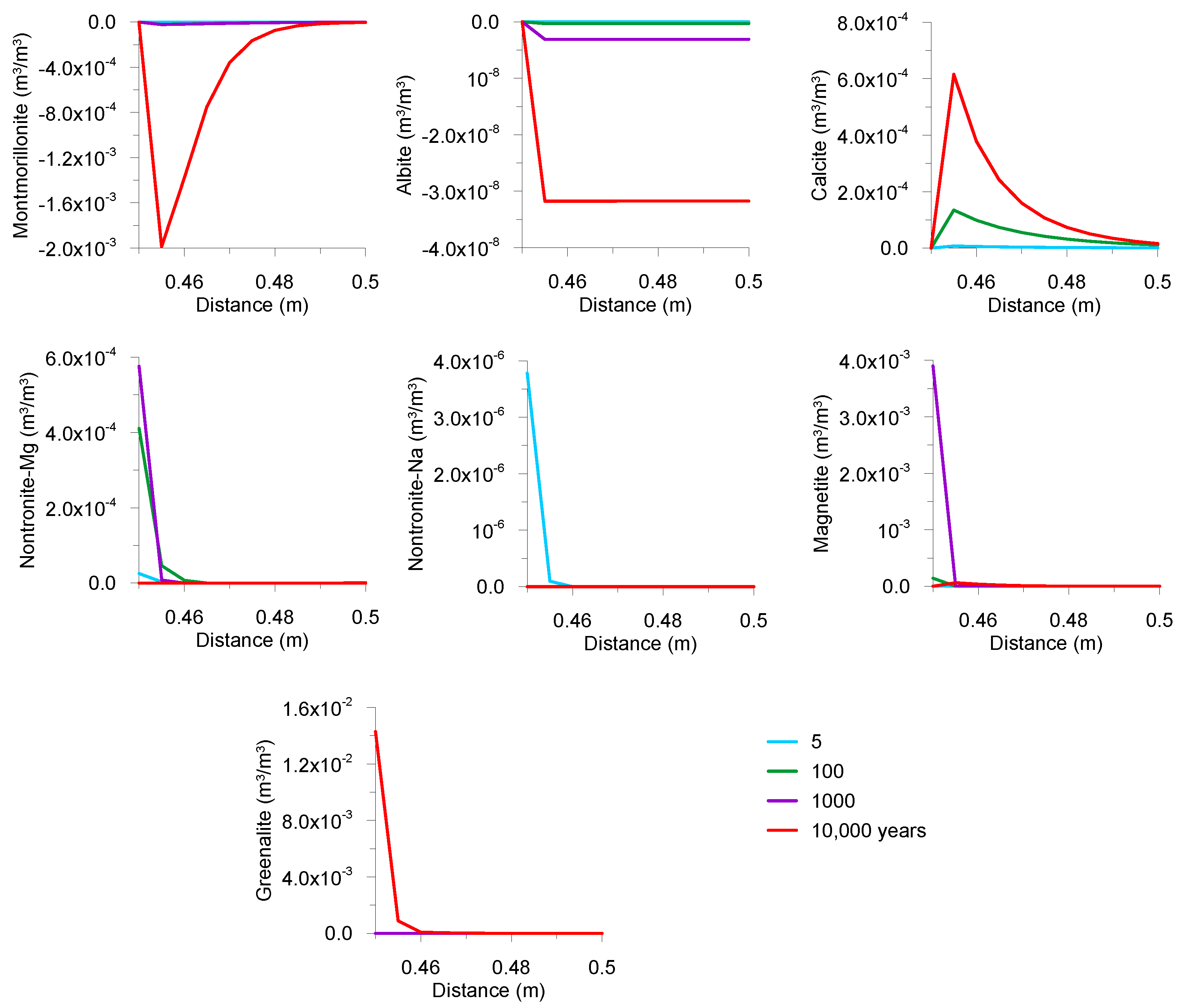
3.2. Mineral Composition of the Bentonite

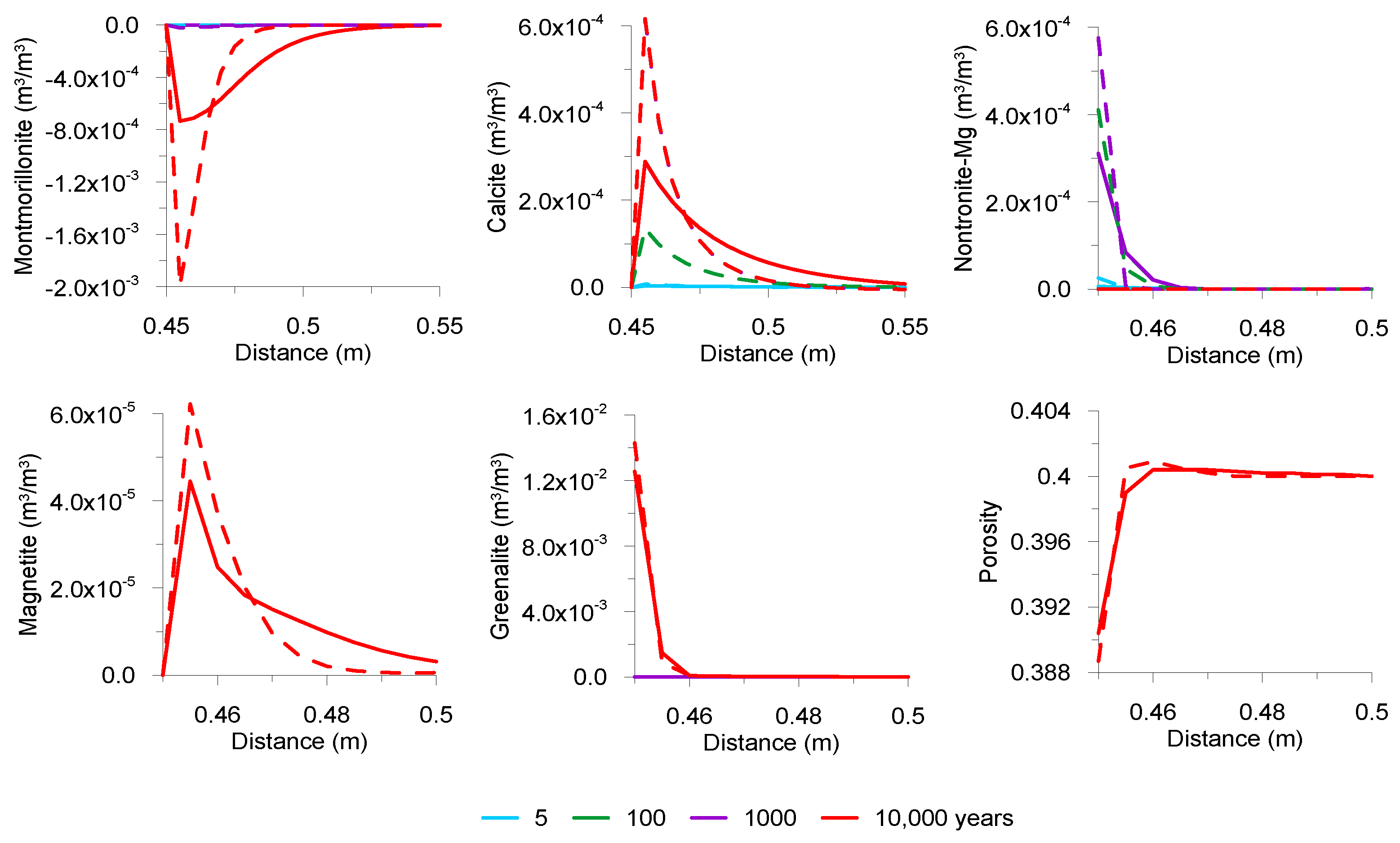
Figure 3 displays the calculated variation of the volumetric fraction of the minerals against distance. Bentonite minerals dissolve because the dissolution of iron provokes an increase in pH that makes silicates unstable. Montmorillonite dissolution releases Ca yielding calcite precipitation, however, specially in the first 100 years, Ca in the montmorillonite interlayer can also be exchanged by Fe and thereby likewise induce calcite precipitation (7.5 $\times {10}^{-6}$ ${\mathrm{m}}^3$${\mathrm{m}}^{-3}$). The volumetric fraction of calcite remains constant from 1000 to 10,000 years indicating no precipitation/dissolution. Dissolution of the primary phases of the bentonite are more important after 10,000 years when the pH is higher. Results from the numerical model show precipitation of nontronite, magnetite and greenalite as secondary phases. At 5 years, specially nontronite-Mg but also nontronite-Na precipitate because there is available Fe and Si in the porewater due to iron and bentonite dissolution, respectively. Magnetite starts precipitating at 100 years, when enough Fe is available. At 1000 years, pH is increasing that provokes the dissolution of nontronite-Na and nontronite-Mg, which release Si and Fe. At the same time, the bentonite minerals and the canister are still dissolving. These conditions lead to greenalite formation. Greenalite is more stable than magnetite under these conditions, therefore, magnetite dissolves. At 10,000 years, greenalite is the main corrosion product. Corrosion products (nontronite, magnetite and greenalite) precipitate quite close to the iron-bentonite interface, and calcite also precipitates along the first 5 cm right after the interface. The reference model predicts neither precipitation of cronstedtite nor that of siderite.

Precipitation of magnetite, calcite and greenalite has been recently found in the Iron Corrosion in Bentonite (IC-A) experiment in the Mont-Terri rock laboratory (Switzerland) [31], which supports our model results. Experiments performed by Schlegel et al. [6,7] and Martin et al. [8] reported the presence of magnetite, cronstedtite and siderite, but our reference model does not predict the formation of siderite or cronstedtite. These reported experiments were performed at 90$°\mathrm{C}$ with Callovo-Oxfordian argilite, which contains about 30 wt% calcite. Thus, the temperature, bentonite and porewater compositions could have a significant impact on the nature of formed corrosion products.

Other modelling works reported in literature, such as Bildstein et al. [13] and Samper et al. [19], predicted the precipitation of cronstedtite and siderite. However, they did not consider greenalite as corrosion product in their numerical models. Therefore, the potential secondary phases selected in the numerical model have an impact on the predicted results. On the other hand, the porewater composition considered had higher ${\mathrm{HCO}}_3^{-}$ concentration in solution allowing siderite precipitation, and the differences in the bentonite composition and temperature of the system could have an effect as well. Although small differences, in general, our results are consistent with other reported models in the literature [13,18,19], where a carbonate phase (calcite or siderite) and Fe-silicate phases (greenalite, nontronite or cronstedtite) will precipitate as corrosion products together with magnetite. The other reported numerical models [13,18,19] consider the canister as porous media, then magnetite prevails as corrosion product precipitating in the canister. However, when iron is considered as boundary [18], Fe-silicates are dominating, which is in agreement with our findings, indicating that bentonite is mainly altered to Fe-silicates rather than to magnetite.

Simulation results are always influenced by certain assumptions and simplifications in the conceptual model. For instance, pyrite forming due to the presence of sulphate-reducing bacteria has been observed in experiments [45]. However, our conceptual model does not consider biological processes, therefore pyrite formation cannot be reproduced. The relevance of microbially induced iron corrosion may, however, be relevant only temporarily as long as the bentonite packing density is not high enough to suppress microbial activity significantly [30,46].

3.3. Porosity

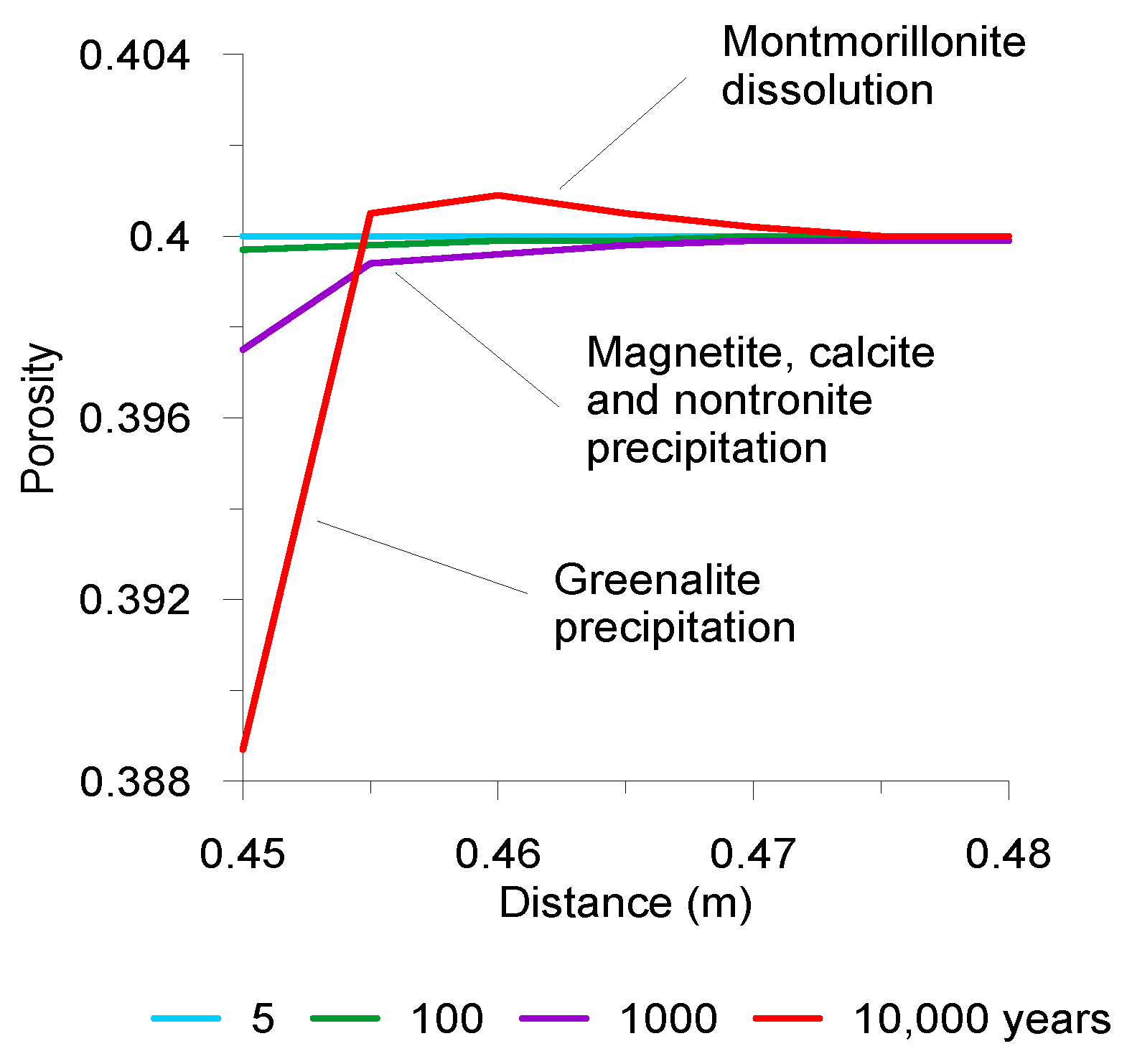
Figure 4 shows the porosity variation at 5 and 10,000 years. The numerical model calculates the total mineral volumetric fraction in each node ($Vf$), ranging from 0 to 1, and the porosity is calculated with the following relationship:

$$\varphi =1-Vf$$

(9)

In general, the model does not predict important changes in porosity, being unnoticeable at 5 years. At 1000 years, the porosity decreases due to the precipitation of magnetite, calcite and nontronite, but especially magnetite forming in larger amounts. At the end of the calculations, at 10,000 years, there is a decrease in porosity right after the interface due to precipitation of greenalite. Although there is also dissolution of bentonite near the interface, precipitation is higher than dissolution thus porosity decreases. Slightly further away from the interface, there is an increase of porosity mainly due to montmorillonite dissolution. Numerical models reported in literature, such as that by Bildstein et al. [13] and Samper et al. [19] predicted pore clogging due to the formation of magnetite followed by an increase of porosity due to dissolution of bentonite. They considered the canister as porous material, thus magnetite, which has larger molar volume (44.52 ${\mathrm{cm}}^3$${\mathrm{mol}}^{-1}$) than iron (7.09 ${\mathrm{cm}}^3$${\mathrm{mol}}^{-1}$), could precipitate clogging the pores. However, our conceptual model considers the canister as boundary, hence, the secondary phases precipitate in the porosity of the bentonite. Dissolution of montmorillonite and precipitation of greenalite take place at the same time, both with similar pore volumes, 133.96 ${\mathrm{cm}}^3$${\mathrm{mol}}^{-1}$ and 115 ${\mathrm{cm}}^3$${\mathrm{mol}}^{-1}$, respectively, therefore, not much changes on porosity are predicted.

4. Sensitivity Analysis

4.1. Corrosion Rate of the Canister

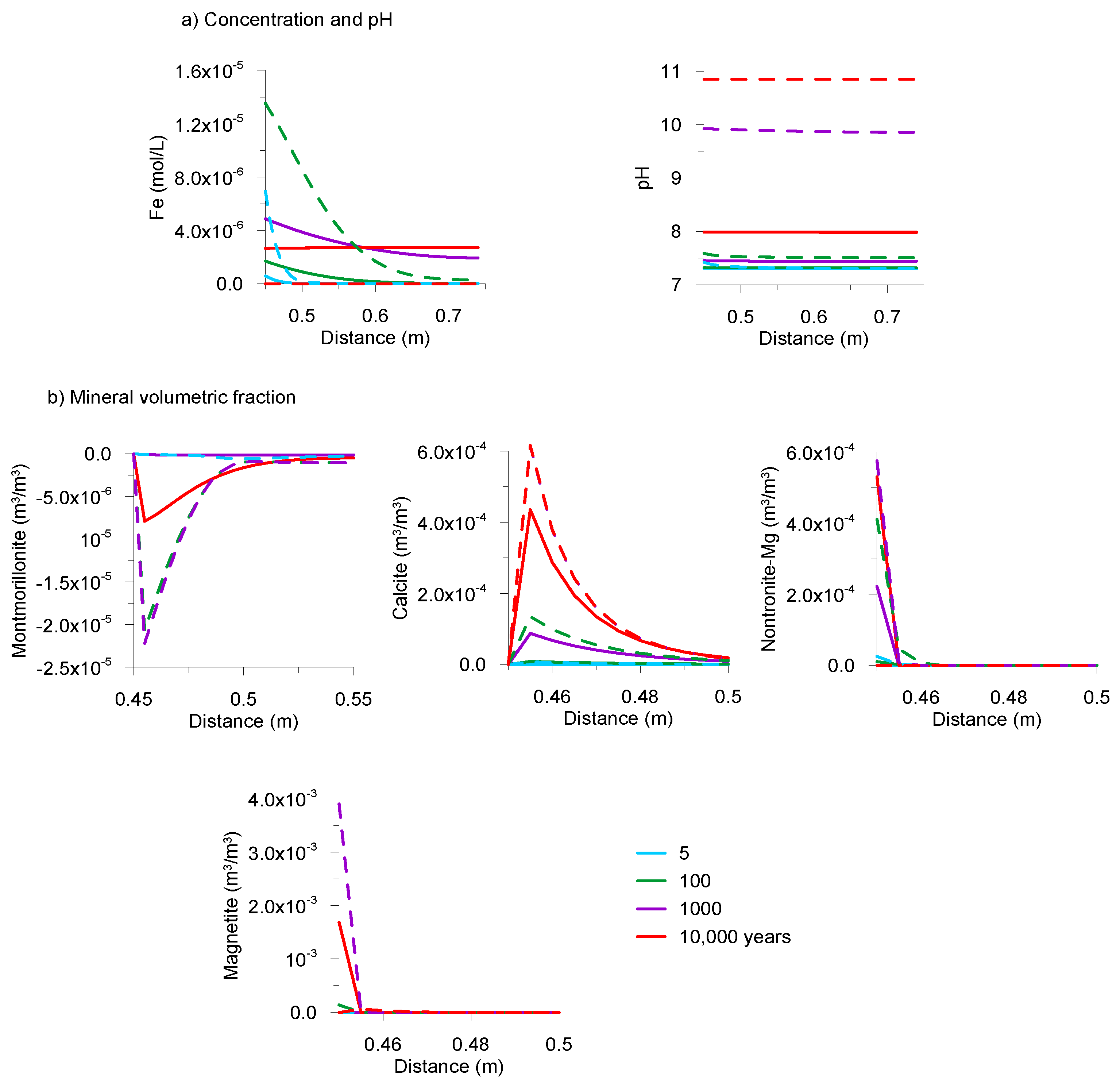
In the real system, it is expected to have larger corrosion rates at the beginning that will decrease with time [22]. The formation of corrosion products at the surface of the canister will result in the formation of a protective layer, which would likely decrease the corrosion rate. Therefore, larger and lower corrosion rates with respect to the reference model have been considered in order to study the effect of the corrosion rate on the formation of secondary phases. In the reference model we assume a constant rate of 2 $\mathsf{\mu }$m ${\mathrm{y}}^{-1}$, which is replaced with a rate of either 10 or 0.1 $\mathsf{\mu }$m ${\mathrm{y}}^{-1}$. Our numerical results are comparable with those reported by Samper et al. [19].

Figure 5 shows the model results considering a constant corrosion rate of 10 $\mathsf{\mu }$m ${\mathrm{y}}^{-1}$. The higher corrosion rate yields a rapid increase in pH, which is then almost constant at 1000 years. This can be explained by the higher dissolution of iron and montmorillonite, consuming protons. In comparison with the reference model, in this model, at 5 years, the Fe concentration in the porewater is higher, yielding a rapid precipitation of secondary phases, and then it decreases with time because of increasing pH, which is linked to secondary phases formation. At 100 years, calcite, nontronite-Mg and magnetite are the main secondary phases, in volumetric fractions larger than in the reference model. The precipitation of greenalite starts earlier and is the principal consumer of Si at 1000 years, and therefore nontronite does not continue forming. At 10,000 years, considerable amount of greenalite forms.

Figure 6 displays the model results considering a constant corrosion rate of 0.1 $\mathsf{\mu }$m ${\mathrm{y}}^{-1}$. In the first 1000 years, the Fe concentration in the porewater increases with time. During this time, Fe(II) species mainly diffuses through the bentonite and adsorbs via cation exchange. However, at 1000 years, it decreases due to precipitation of corrosion products. The pH is barely increasing with time reaching a maximum value of 8. Therefore, bentonite does not dissolve much. Calcite precipitates more noticeably at 1000 years due to Fe(II)/Ca(II) cation exchange within the montmorillonite interlayer, and at 10,000 years, calcite precipitates due to the Ca coming from the montmorillonite dissolution. Nontronite precipitates due to the available Fe and Si in the porewater, however, at 10,000 years, Fe is mainly consumed by magnetite precipitation. The numerical model does not predict precipitation of other corrosion products such as greenalite, because there is not enough Fe and Si in the system to let greenalite precipitate due to the low dissolution of bentonite and low corrosion rate. In this model, the predicted alteration thickness is larger because diffusion dominates rather than mineral dissolution–precipitation processes. The cation exchange is relevant for the first 1000 years when there is not much precipitation of magnetite.

4.2. Diffusion Coefficient

Other authors working on similar systems used a larger pore diffusion coefficient for the bentonite [18]. In order to study the impact of the diffusion coefficient on the formation of corrosion products, we assumed a pore diffusion coefficient being six times higher (6 $\times {10}^{-10}$ ${\mathrm{m}}^2$ ${\mathrm{s}}^{-1}$), which is the same as used by Wilson et al. [18]. This model considers the same corrosion rate as in the reference model (2 $\mathsf{\mu }$m ${\mathrm{y}}^{-1}$). Model results are shown in Figure 7. In comparison with the reference model, a higher diffusion coefficient gives a larger thickness of the altered bentonite, which has also been reported by Samper et al. [19]. Ca released from bentonite dissolution is transported away and therefore gives a larger thickness of calcite precipitation. The Si supply from bentonite also gives a larger precipitation area for nontronite and greenalite. The thickness of the porosity alteration is larger, however, there is less variation in porosity because there is higher diffusion of dissolved species away from the corroding iron.

4.3. Porewater

There is disagreement in literature about how to determine the initial composition of the porewater of the bentonite, because it is not easy to obtain a reliable composition. Thus, we study the effect of the porewater composition on the nature of formed corrosion products. The composition considered (

Table 8. Initial porewater composition used in the sensitivity analysis.

Component	Water Composition (mol ${\mathbf{L}}^{-1}$)
Al${\left(\mathrm{OH}\right)}_4^{-}$	1.00 $\times {10}^{-8}$
${\mathrm{Ca}}^{2+}$	1.52 $\times {10}^{-4}$
${\mathrm{Cl}}^{-}$	3.95 $\times {10}^{-4}$
${\mathrm{Fe}}^{+2}$	1.79 $\times {10}^{-8}$
${\mathrm{HCO}}_3^{-}$	5.05 $\times {10}^{-3}$
${\mathrm{K}}^{+}$	5.37 $\times {10}^{-5}$
${\mathrm{Mg}}^{2+}$	1.60 $\times {10}^{-4}$
${\mathrm{Na}}^{+}$	4.35 $\times {10}^{-3}$
${\mathrm{SiO}}_2$(aq)	3.76 $\times {10}^{-4}$
${\mathrm{SO}}_4^{2-}$	1.56 $\times {10}^{-5}$
${\mathrm{O}}_2$(aq)	1.00 $\times {10}^{-15}$
pH	7.83

) corresponds to a granitic porewater reported by Samper et al. [19]. This porewater composition has been selected because it contains the concentration of all primary species used in our model and higher Si content. In this case, the porewater is not at equilibrium with the montmorillonite. The interaction of low mineralized groundwater with bentonite is investigated in scenarios simulating the intrusion of glacial melt water into emplacement caverns of a repository in crystalline rock (see, e.g., Bouby et al. [47]).

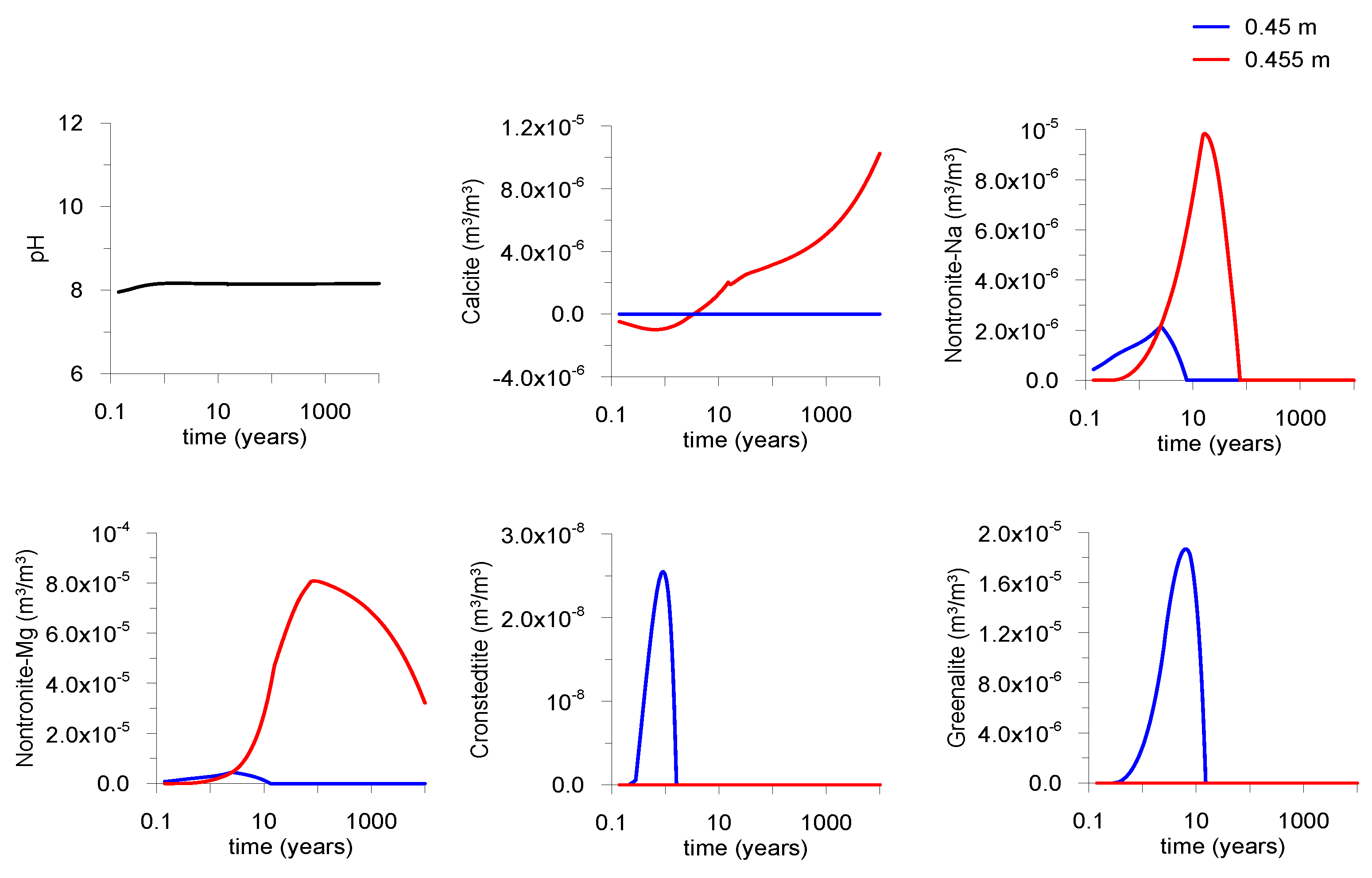
Figure 8 shows the results calculated for the numerical model. The pH remains constant around a value of 8. In this system, the Fe-silicates are the main corrosion products and no precipitation of magnetite is predicted. Calcite precipitates during the 10,000 years due to Ca/Fe(II) exchange. Nontronite-Na, cronstedtite and greenalite precipitate during the first 10 years. However, afterwards they dissolve and the Fe and Si are consumed by precipitation of nontronite-Mg, which remains until the end of the run (10,000 years). Thus, our model results suggest that the porewater composition can affect the nature of corrosion products, being Fe-silicates as main corrosion products. Our numerical model results differ from that from Samper et al. [19] because of different assumptions in the conceptual model, such as the selected secondary phases, considering the canister as porous material and a boundary flow.

4.4. Reactive Surface Area

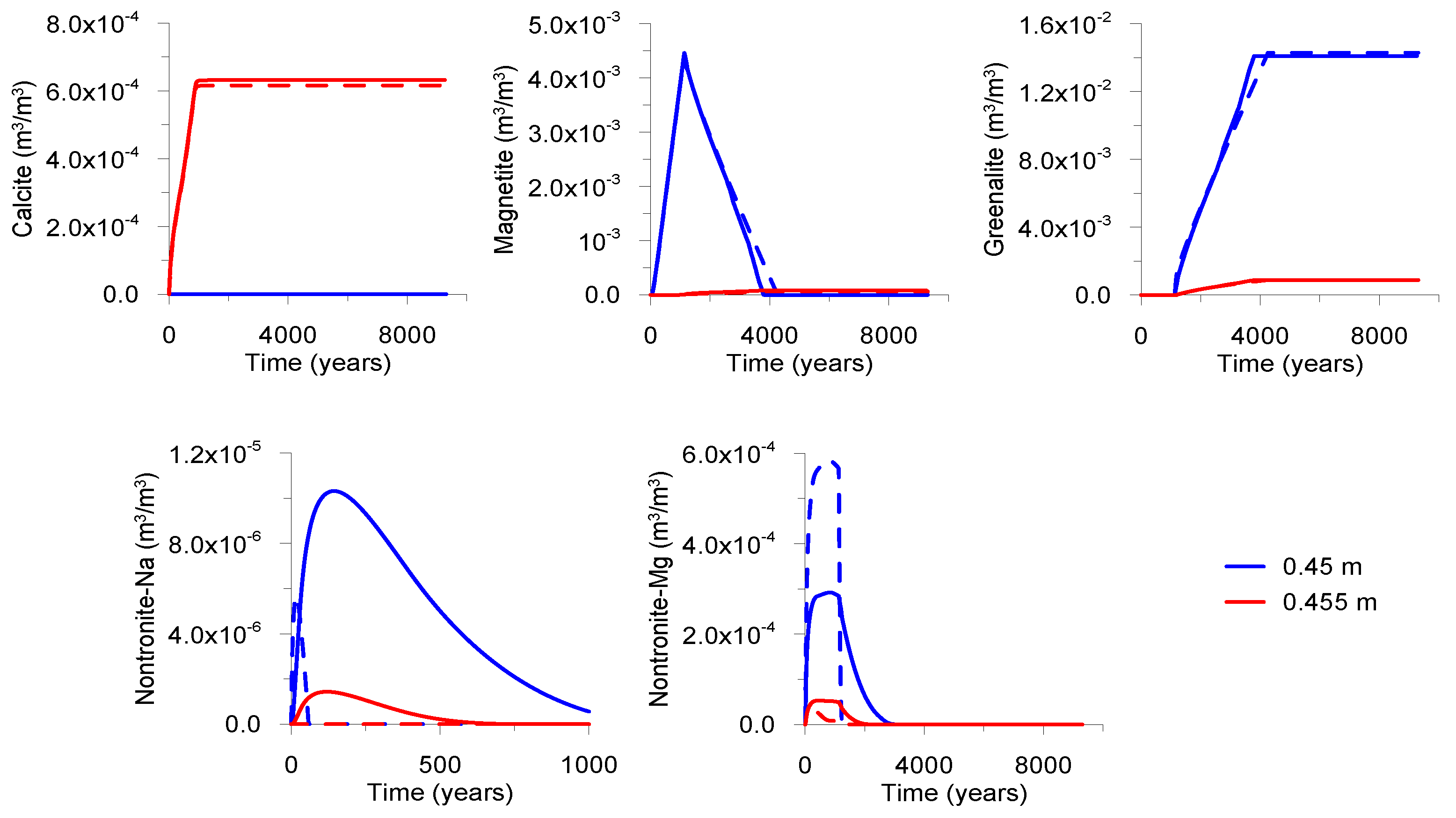
In the reference model, large reactive surface areas ($\sigma$ = 1000 ${\mathrm{m}}^2$/${\mathrm{m}}^3$) have been used for the secondary phases in order to let them precipitate at equilibrium. However, a sensitivity analysis on the surface area has been done, using a much lower value ($\sigma$ = 0.1 ${\mathrm{m}}^2$/${\mathrm{m}}^3$). Figure 9 shows the calculated evolution of volumetric fraction of the secondary phases. Calcite, magnetite, nontronite-Mg and nontronite-Na precipitate within the first 1000 years. However, afterwards, magnetite and nontronites dissolve, while the volumetric fraction of calcite remains constant. Magnetite dissolves slowly within 3000 years, after that no magnetite remains in the first node (interface), and only 6 $\times {10}^{-5}$ ${\mathrm{m}}^3$${\mathrm{m}}^{-3}$ remains in the following nodes (see Figure 3). Nontronites dissolve rapidly, not only the first node, but also in the following nodes. At the same time, greenalite starts precipitating consuming the Fe and Si of the system. In general, a lower reactive surface area does not give important changes compared to the reference model for calcite, magnetite and greenalite, because although the low kinetics they reach the equilibrium. However, the lower surface area provokes a delay on time on nontronite precipitation, because more time is needed to reach the equilibrium.

4.5. Longer Interaction Time

The reference model considers an iron-bentonite interaction of 10,000 years because it is the time expected that the canister should resist failure [48]. However, due to the slow kinetics of the primary minerals dissolution, longer interaction times can cause more dissolution of them, and therefore, more precipitation of secondary phases. Thus, the effect of a 100,000 years interaction is also studied, taking into account the same corrosion rate as in the reference model (2 $\mathsf{\mu }$m ${\mathrm{y}}^{-1}$). Figure 10 displays the calculated volumetric fractions only for the minerals that present some variations with respect to the reference model (albite, magnetite and cronstedtite). From the period of time between 10,000 and 100,000 years, the volumetric fraction of montmorillonite remains constant, therefore the volumetric fraction of calcite is also constant. However, the dissolution of albite and quartz increase with time. This Si supply could inhibit montmorillonite dissolution [49,50], and is consumed by precipitation of cronstedtite (1.8 $\times {10}^{-5}$ ${\mathrm{m}}^3$ ${\mathrm{m}}^{-3}$), which precipitates not only near to the interface, but extends into the bentonite. Magnetite slightly dissolves, at 10,000 years the predicted volumetric fraction is 6 $\times {10}^{-5}$ ${\mathrm{m}}^3$ ${\mathrm{m}}^{-3}$ and at 100,000 years is 5 $\times {10}^{-5}$ ${\mathrm{m}}^3$ ${\mathrm{m}}^{-3}$. Even for longer interaction times and with the formation of cronstedtite, the main corrosion product of the system at the end of the run (100,000 years) is greenalite, being the same as that in the reference model.

5. Conclusions

A 1D radial reactive transport model has been developed in order to better understand the processes occurring in the long-term iron–bentonite interaction. Results suggest that Fe partly diffuses and is partly adsorbed to montmorillonite by cation exchange, in the short-term. In the long-term, Fe is mainly consumed by corrosion products formation. Calcite precipitates due to the release of Ca into the porewater, in the short-term because of cation exchange, and in the long-term because of montmorillonite dissolution. The reference model predicts precipitation of nontronite, magnetite and greenalite as corrosion products. In the short-term, nontronite and magnetite form consuming the Fe and Si of the system, however, in the long-term, greenalite is predicted as main corrosion product forming upon alteration of the bentonite. Due to the slow kinetics of the minerals, not much mineral dissolution/precipitation is predicted, and therefore, the variation of porosity is not relevant. However, porosity slightly decreases near the interface due to precipitation of mainly greenalite, and increases thereafter because of montmorillonite dissolution.

Results of the sensitivity analysis show that a larger corrosion rate would provoke a rapid precipitation of greenalite due to the rapid Si supply from the dissolution of bentonite. On the contrary, when a lower corrosion rate is considered, the model predicts slower dissolution of bentonite, hence, only nontronite and magnetite precipitate. When a larger diffusion coefficient is considered, the transport of dissolved Fe(II) species dominates with less mineral dissolution/precipitation occurring. The porewater composition can affect the nature of corrosion products formed, Fe-silicates being more relevant than magnetite. A lower reactive surface area for the secondary phases does not seem to have an important impact. Longer iron–bentonite interaction time allows higher dissolution of bentonite, thus cronstedtite forms coexisting with calcite, magnetite and greenalite.

Overall, outcomes suggest that the predicted main corrosion products on the long-term are Fe-silicates minerals. Such phases thus should deserve further attention as chemical barrier in the diffusion of radionuclides to the repository far field. Our results can differ from other reactive transport calculations reported in the literature because of the assumptions considered in the conceptual model, such as the selected secondary phases, considering the canister as porous material or the temperature of the system.

References

- Savage, D. Prospects for Coupled Modelling; Technical Report, STUK-TR 13; Radiation and Nuclear Safety Authority: Helsinki, Finland, 2012. [Google Scholar]
- Bildstein, O.; Claret, F. Chapter 5—Stability of Clay Barriers Under Chemical Perturbations. In Natural and Engineered Clay Barriers; Developments in Clay Science; Tournassat, C., Steefel, C.I., Bourg, I.C., Bergaya, F., Eds.; Elsevier: Amsterdam, The Netherlands, 2015; Volume 6, pp. 155–188. [Google Scholar] [CrossRef]
- Claret, F.; Marty, N.; Tournassat, C. Modeling the Long-Term Stability of Multibarrier Systems for Nuclear Waste Disposal in Geological Clay Formations. In Reactive Transport Modeling; Xiao, Y., Whitaker, F., Xu, T., Steefel, C., Eds.; John Wiley & Sons, Ltd.: Chichester, UK, 2018; pp. 395–436. [Google Scholar]
- Bildstein, O.; Claret, F.; Frugier, P. RTM for Waste Repositories. Rev. Mineral. Geochem. 2019, 85, 419–457. [Google Scholar] [CrossRef] [Green Version]
- Deissmann, G.; Mouheb, N.A.; Martin, C.; Turrero, M.; Torres, E.; Kursten, B.; Weetjens, E.; Jacques, D.; Cuevas, J.; Samper, J.; et al. Experiments and Numerical Model Studies on Interfaces; Final version as of 11.05.2021 of Deliverable D2.5 of the HORIZON 2020 Project EURAD. EC Grant Agreement no: 847593. 2021. [Google Scholar]
- Schlegel, M.L.; Bataillon, C.; Benhamida, K.; Blanc, C.; Menut, D.; Lacour, J.L. Metal corrosion and argillite transformation at the water-saturated, high-temperature iron-clay interface: A microscopic-scale study. Appl. Geochem. 2008, 23, 2619–2633. [Google Scholar] [CrossRef]
- Schlegel, M.L.; Bataillon, C.; Brucker, F.; Blanc, C.; Prêt, D.; Foy, E.; Chorro, M. Corrosion of metal iron in contact with anoxic clay at 90 °C: Characterization of the corrosion products after two years of interaction. Appl. Geochem. 2014, 51, 1–4. [Google Scholar] [CrossRef]
- Martin, F.; Bataillon, C.; Schlegel, M. Corrosion of iron and low alloyed steel within a water saturated brick of clay under anaerobic deep geological disposal conditions: An integrated experiment. J. Nucl. Mater. 2008, 379, 80–90. [Google Scholar] [CrossRef]
- Kaufhold, S.; Schippers, A.; Marx, A.; Dohrmann, R. SEM study of the early stages of Fe-bentonite corrosion—The role of naturally present reactive silica. Corros. Sci. 2020, 171, 108716. [Google Scholar] [CrossRef]
- Savage, D.; Watson, C.; Benbow, S.; Wilson, J. Modelling iron-bentonite interactions. Appl. Clay Sci. 2010, 47, 91–98. [Google Scholar] [CrossRef]
- Samper, J.; Lu, C.; Montenegro, L. Reactive transport model of interactions of corrosion products and bentonite. Phys. Chem. Earth Parts A/B/C 2008, 33, S306–S316. [Google Scholar] [CrossRef]
- Lu, C.; Samper, J.; Fritz, B.; Clement, A.; Montenegro, L. Interactions of corrosion products and bentonite: An extended multicomponent reactive transport model. Phys. Chem. Earth Parts A/B/C 2011, 36, 1661–1668. [Google Scholar] [CrossRef]
- Bildstein, O.; Trotignon, L.; Perronnet, M.; Jullien, M. Modelling iron-clay interactions in deep geological disposal conditions. Phys. Chem. Earth Parts A/B/C 2006, 31, 618–625. [Google Scholar] [CrossRef]
- Wersin, P.; Birgersson, M.; Olsson, O.; Karnland, O.; Snellman, M. Impact of Corrosion-Derived Iron on the Bentonite Buffer within the KBS-3H Disposal Concept The Olkiluoto Site as Case Study; Technical Report SKB-TR-08-34; Swedish Nuclear Fuel and Waste Management Co.: Stockholm, Sweden, 2008. [Google Scholar]
- Marty, N.C.; Fritz, B.; Clément, A.; Michau, N. Modelling the long term alteration of the engineered bentonite barrier in an underground radioactive waste repository. Appl. Clay Sci. 2010, 47, 82–90. [Google Scholar] [CrossRef]
- Wersin, P.; Birgersson, M. Reactive transport modelling of iron-bentonite interaction within the KBS-3H disposal concept—The Olkiluoto site as case study. Geol. Soc. Spec. Publ. 2014, 400, 237–250. [Google Scholar] [CrossRef]
- Ngo, V.V.; Delalande, M.; Clément, A.; Michau, N.; Fritz, B. Coupled transport-reaction modeling of the long-term interaction between iron, bentonite and Callovo-Oxfordian claystone in radioactive waste confinement systems. Appl. Clay Sci. 2014, 101, 430–443. [Google Scholar] [CrossRef]
- Wilson, J.C.; Benbow, S.; Sasamoto, H.; Savage, D.; Watson, C. Thermodynamic and fully-coupled reactive transport models of a steel-bentonite interface. Appl. Geochem. 2015, 61, 10–28. [Google Scholar] [CrossRef]
- Samper, J.; Naves, A.; Montenegro, L.; Mon, A. Reactive transport modelling of the long-term interactions of corrosion products and compacted bentonite in a HLW repository in granite: Uncertainties and relevance for performance assessment. Appl. Geochem. 2016, 67, 42–51. [Google Scholar] [CrossRef]
- Montes-H, G.; Marty, N.; Fritz, B.; Clement, A.; Michau, N. Modelling of long-term diffusion–reaction in a bentonite barrier for radioactive waste confinement. Appl. Clay Sci. 2005, 30, 181–198. [Google Scholar] [CrossRef]
- Finsterle, S.; Muller, R.A.; Baltzer, R.; Payer, J.; Rector, J.W. Thermal Evolution near Heat-Generating Nuclear Waste Canisters Disposed in Horizontal Drillholes. Energies 2019, 12, 596. [Google Scholar] [CrossRef] [Green Version]
- Necib, S.; Diomidis, N.; Keech, P.; Nakayama, M. Corrosion of Carbon Steel in Clay Environments Relevant to Radioactive Waste Geological Disposals, Mont Terri Rock Laboratory (Switzerland); Springer International Publishing: Cham, Switzerland, 2018; pp. 331–344. [Google Scholar] [CrossRef]
- Carrière, C.; Dillmann, P.; Foy, E.; Neff, D.; Dynes, J.; Linard, Y.; Michau, N.; Martin, C. Use of nanoprobes to identify iron-silicates in a glass/iron/argillite system in deep geological disposal. Corros. Sci. 2019, 158, 108104. [Google Scholar] [CrossRef] [Green Version]
- Saaltink, M.W.; Batlle, F.; Ayora, C.; Carrera, J.; Olivella, S. RETRASO, a code for modeling reactive transport in saturated and unsaturated porous media. Geol. Acta 2004, 2, 235–251. [Google Scholar]
- Olivella, S.; Gens, A.; Carrera, J.; Alonso, E.E. Numerical formulation for a simulator (CODE_BRIGHT) for the coupled analysis of saline media. Eng. Comput. 1996, 13, 87–112. [Google Scholar] [CrossRef] [Green Version]
- Bossart, P.; Bernier, F.; Birkholzer, J.; Bruggeman, C.; Connolly, P.; Dewonck, S.; Fukaya, M.; Herfort, M.; Jensen, M.; Matray, J.; et al. Mont Terri Rock Laboratory, 20 Years of Research: Introduction, Site Characteristics and Overview of Experiments; Birkhäuser: Cham, Swizerland, 2018; Volume 5. [Google Scholar] [CrossRef]
- Zheng, L.; Rutqvist, J.; Birkholzer, J.T.; Liu, H.H. On the impact of temperatures up to 200 °C in clay repositories with bentonite engineer barrier systems: A study with coupled thermal, hydrological, chemical, and mechanical modeling. Eng. Geol. 2015, 197, 278–295. [Google Scholar] [CrossRef] [Green Version]
- King, F. Corrosion of Carbon Steel under Anaerobic Conditions in a Repository for SF and HLW in Opalinus Clay; Technical Report NAGRA-NTB–08-12; National Cooperative for the Disposal of Radioactive Waste: Wettingen, Switzerland, 2008. [Google Scholar]
- Zheng, L.; Rutqvist, J.; Xu, H.; Birkholzer, J.T. Coupled THMC models for bentonite in an argillite repository for nuclear waste: Illitization and its effect on swelling stress under high temperature. Eng. Geol. 2017, 230, 118–129. [Google Scholar] [CrossRef] [Green Version]
- Smart, N.R.; Reddy, B.; Rance, A.P.; Nixon, D.J.; Frutschi, M.; Bernier-Latmani, R.; Diomidis, N. The anaerobic corrosion of carbon steel in compacted bentonite exposed to natural Opalinus Clay porewater containing native microbial populations. Corros. Eng. Sci. Technol. 2017, 52, 101–112. [Google Scholar] [CrossRef] [Green Version]
- Morelová, N.; Schild, D.; Heberling, F.; Finck, N.; Dardenne, K.; Metz, V.; Geckeis, H. Anaerobic Corrosion of Carbon Steel in Compacted Bentonite Exposed to Natural Opalinus Clay Porewater: Bentonite Alteration Study. Goldschmidt Virtual, 4–9 July 2021. [Google Scholar]
- Karnland, O. Chemical and Mineralogical Characterization of the Bentonite Buffer for the Acceptance Control Procedure in a KBS-3 Repository; Technical Report SKB-TR-10-60; Department of Energy, Office of Scientific and Technical Information: Oak Ridge, TN, USA, 2010. [Google Scholar]
- Kiviranta, L.; Kumpulainen, S.; Pintado, X.; Karttuten, P.; Schatz, T. Characterization of Bentonite and Clay Materials 2012–2015; Working Report 2016-05; POSIVA OY: Eurajoki, Finland, 2018. [Google Scholar]
- Reddy, B.; Padovani, C.; Smart, N.R.; Rance, A.P.; Cook, A.; Milodowski, A.; Field, L.; Kemp, S.; Diomidis, N. Further results on the in situ anaerobic corrosion of carbon steel and copper in compacted bentonite exposed to natural Opalinus Clay porewater containing native microbial populations. Mater. Corros. 2021, 72, 268–281. [Google Scholar] [CrossRef]
- Curti, E. Modelling Bentonite Pore Waters for the Swiss High-Level Radioactive Waste Repository; Technical Report, PSI Report No. 93-05; PSI: Villigen, Switzerland, 1993. [Google Scholar]
- Melkior, T.; Mourzagh, D.; Yahiaoui, S.; Thoby, D.; Alberto, J.; Brouard, C.; Michau, N. Diffusion of an alkaline fluid through clayey barriers and its effect on the diffusion properties of some chemical species. Appl. Clay Sci. 2004, 26, 99–107. [Google Scholar] [CrossRef]
- Johnson, J.; Lundeen, S. GEMBOCHS Thermodynamic Datafiles for Use with the EQ3/6 Software Package; Technical Report, Yucca Mountain Laboratory, Milestone Report M0L72; Lawrence Livermore National Laboratory: Livermore, CA, USA, 1994. [Google Scholar]
- Appelo, C.; Postma, D. Geochemistry, Groundwater and Pollution; A.A. Balkema: Rotterdam, The Netherland, 2005. [Google Scholar]
- Lasaga, A.C. Chemical kinetics of water-rock interactions. J. Geophys. Res. Solid Earth 1984, 89, 4009–4025. [Google Scholar] [CrossRef]
- Cama, J.; Ganor, J.; Ayora, C.; Lasaga, C. Smectite dissolution kinetics at 80 °C and pH 8.8. Geochim. Cosmochim. Acta 2000, 64, 2701–2717. [Google Scholar] [CrossRef]
- Dove, P.M. The dissolution kinetics of quartz in aqueous mixed cation solutions. Geochim. Cosmochim. Acta 1999, 63, 3715–3727. [Google Scholar] [CrossRef]
- Knauss, K.G.; Wolery, T.J. Dependence of albite dissolution kinetics on ph and time at 25 °C and 70 °C. Geochim. Cosmochim. Acta 1986, 50, 2481–2497. [Google Scholar] [CrossRef]
- Kamei, G.; Ohmoto, H. The kinetics of reactions between pyrite and O2-bearing water revealed from in situ monitoring of DO, Oh and pH in a closed system. Geochim. Cosmochim. Acta 2000, 64, 2585–2601. [Google Scholar] [CrossRef]
- Plummer, L.; Parkhurst, D.; Wigley, T. Critical review of the kinetics of calcite dissolution and precipitation. In Chemical Modeling of Aqueous Systems; ACS Symposium Series: Washington, DC, USA, 1979. [Google Scholar] [CrossRef]
- Necib, S.; Schlegel, M.L.; Bataillon, C.; Daumas, S.; Diomidis, N.; Keech, P.; Crusset, D. Long-term corrosion behaviour of carbon steel andstainless steel in Opalinus clay: Influence of stepwise temperature increase. Corros. Eng. Sci. Technol. 2019, 54, 516–528. [Google Scholar] [CrossRef]
- King, F.; Padovani, C. Review of the corrosion performance of selected canister materials for disposal of UK HLW and/or spent fuel. Corros. Eng. Sci. Technol. 2011, 46, 82–90. [Google Scholar] [CrossRef]
- Bouby, M.; Kraft, S.; Kuschel, S.; Geyer, F.; Moisei-Rabung, S.; Schäfer, T.; Geckeis, H. Erosion dynamics of compacted raw or homoionic MX80 bentonite in a low ionic strength synthetic water under quasi-stagnant flow conditions. Appl. Clay Sci. 2020, 198, 105797. [Google Scholar] [CrossRef]
- National Cooperative for the Disposal of Radioactive Waste (NAGRA). W.S. Project Opalinus Clay—Safety Report—Demonstration of Disposal Feasibility for Spent Fuel, Vitrified High-Level Waste and Long-Lived Intermediate-Level Waste (Entsorgungsnachweis); Technical Report NTB-02-05; Nagra: Wettingen, Switzerland, 2002. [Google Scholar]
- Arthur, R.; Savage, D. Long-Term Stability of Clay Minerals in the Buffer and Backfill; Technical Report, STUK Report STUK-TR22; Finnish Radiation and Nuclear Safety Authority (STUK): Helsinki, Finland, 2016. [Google Scholar]
- Savage, D.; Cloet, V. A Review of Cement-Clay Modelling; Working Report NAB-18-24; Nagra: Wettingen, Switzerland, 2018. [Google Scholar]
Figure 1.
Geometry and materials of the 1D radial model. The axisymmetric model only considers the canister-bentonite interface, at x = 0.45 m, and a thickness of 0.3 m of bentonite, from x = 0.45 to x = 0.75 m.
Figure 2.
Concentration of dissolved species in the porewater and of adsorbed species against distance for the reference model ( = 2 m ). The interface between steel and bentonite is at 0.45 m. Results after 5, 100, 1000 and 10,000 years of interaction are compared.
Figure 3.
Volumetric fraction of minerals versus distance for the reference model ( = 2 m ). For the primary phases (montmorillonite, albite and calcite) the variation of the volumetric fraction is plotted. Positive values mean precipitation and negative values mean dissolution. The interface between steel and bentonite is at 0.45 m. Results at 5, 100, 1000 and 10,000 years of interaction are compared.
Figure 4.
Porosity against length for the reference model ( = 2 m ). The interface between steel and bentonite is at 0.45 m. Results at 5, 100, 1000, and 10,000 years of interaction are compared.
Figure 5.
Results for the numerical model with a corrosion rate of 10 m (continuous lines) are compared with those from the reference model (r = 2 m , dashed lines). The interface between steel and bentonite is at 0.45 m. Results at 5, 100, 1000 and 10,000 years of interaction are given. (a) Fe concentration and pH against distance and (b) volumetric fraction of minerals versus distance. For the primary phases (montmorillonite and calcite) the variation of the volumetric fraction is plotted. Positive values mean precipitation and negative values mean dissolution.
Figure 6.
Results of the numerical model with a corrosion rate of 0.1 m (continuous lines) are compared with those from the reference model (r = 2 m , dashed lines). The interface between steel and bentonite is at 0.45 m. Results at 5, 100, 1000 and 10,000 years of interaction are compared. (a) Fe concentration and pH against distance. (b) Volumetric fraction of minerals versus distance. For the primary phases (montmorillonite and calcite) a variation of the volumetric fraction is plotted. Positive values mean precipitation and negative values mean dissolution. The reference model results for montmorillonite at 10,000 are not plotted (see Figure 3 for that detail).
Figure 7.
Results of the numerical model with a diffusion coefficient of 6 ( = 2 m ) (continuous line) are compared with those from the reference model (dashed line). Volumetric fraction of minerals and porosity versus distance. For the primary phases (montmorillonite and calcite) the variation of the volumetric fraction is plotted. Positive values mean precipitation and negative values mean dissolution. The interface between steel and bentonite is at 0.45 m. Results at 5, 100, 1000 and 10,000 years of interaction are compared. For magnetite and porosity only results at 10,000 years are plotted.
Figure 8.
Evolution of pH and volumetric fraction of secondary phases at two distances from the steel/bentonite interface considering a granitic porewater ( = 2 m ).
Figure 9.
Evolution of the volumetric fraction of the secondary phases of the model with a low reactive surface area ( = 0.1 /, continuous lines) compared with the reference model ( = 1000 /, dashed lines). Results of the node at the interface (0.45 m) and the node right after the interface (0.455 m) are plotted.
Figure 10.
Volumetric fraction of minerals of the model with 100,000 years interaction ( = 2 m ). For albite the variation of the volumetric fraction is plotted. Positive values mean precipitation and negative values mean dissolution. The interface between steel and bentonite is at 0.45 m. Results at 10,000 and 100,000 years of interaction are compared.