Infiltration Depth of Mineral Particles in Gravel-Bed Rivers

Abstract

This article discusses the results of an experimental study of a spill of mineral particles in gravel-bed rivers due to mining accidents. The purpose of this research is to characterize the dynamics of the fine mining particles spilled on a bed of immobilized gravel as a hyper-concentrated mixture and to experimentally characterize the infiltration phenomenon. We analyzed the type of infiltration considering the dimensionless coarse to fine particle size relationship, the dimensionless weight of the fine particles, the relative density of the particles, and the relationship between the subsurface and surface velocities, in addition to the densimetric Froude and Reynolds numbers of the fine particles. We found that the dimensionless infiltration depth is not associated with hydraulic parameters or the weight of the fine sediment spilled; however, fine sediment deposition decreases with depth, and infiltration depth may increase if subsurface flow decreases over time. Finally, a relationship of the dimensionless maximum infiltration depth with the relative density of the mining particles, the ratio of the bed sediment and the mining particles sizes, and the ratio between the subsurface and surface velocities is established.

1. Introduction

Heavy metals in riverbeds can come from acid rock drainage formation, mining, industry, or mining accidents. As a result of current and historical metal mining, rivers and floodplains in many parts of the world have become contaminated by the metal-rich waste in concentrations that may pose a hazard to human and animal livelihoods [1,2,3]. Human health and environmental impacts commonly arise due to the long residence time of heavy metals in river sediments and alluvial soils and their bioaccumulatory nature in plants and animals [2].

Coulthard et al. [1] modeled heavy metal contamination in river systems in the United Kingdom. Simulations considered sediment transport dynamics to analyze contaminant transport due to sediment movement. An increase in flow rate may reduce contamination because it could generate bedload transport, and further dilution may occur. Jaskuła et al. [4] analyzed the spatial variability of riverbed pollution by heavy metals, such as Cr, Ni, Cu, Zn, Cd, and Pb, in sediments of the Warta riverbed in Poland. They found that the highest contributors to pollution were urbanized areas and industrial activities. They also reported the temporal variability of heavy metals and that the ecological risk is proportional to the presence of heavy metals in the riverbed.

Several mining accidents have occurred worldwide. Benito et al. [5] studied the Aznalcollar mine spill in 1998. The accident caused the spilling of some 4.5 × 10${}^3$ Mm${}^3$ of acid water and pyrite ore, generating a waste sludge with a high concentration of heavy metals in the floodplains of the Agrio and Guadiamar rivers, Spain, affecting the Sierra Morena ecosystem. In 2014 the tailings dam failure at the Mount Polley Mine accidentally spilled 25 Mm${}^3$ into the Quesnel River watershed, and the material was deposited within the riparian zone. However, metal concentrations were lower than in other mining accidents [6]. The collapse of the Fundão tailings dam, Brazil, in 2015, spilled more than 43 Mm${}^3$ of iron ore tailings, polluting a length of approximately 668 km from the Doce River to the Atlantic Ocean. Part of the tailings affected the nature reserve in the Doce River [7]. In Chile have occurred several mining accidents of pipe failure that have ended with copper concentrate or tailings into gravel rivers. Cenma [8] reported sedimentary chemical analysis of the Aconcagua river, finding a negative effect associated with the presence of heavy metals along the river due to mining activity. The most critical situation occur during the fall. Soublette and Heyer [9] confirmed sediments with the presence of contaminants, both gold and copper ore tailings on the Illapel river, Chile. These contaminants generated poor quality surface water, but there was no evidence of groundwater contamination.

The hyporheic zone allows exchange between the groundwater system and surface water in rivers and floodplains. This exchange takes place through sediment porosity and is characterized by the circulation of surface water into the alluvium and back to the riverbed [10]. In highly permeable gravel beds, interstitial flow velocities can transport fine particles into the hyporheic zone, filling interstitial spaces [11,12], so gravel porosity is a reservoir for interstitial deposition of fine sediment [13]. Fine particles in gravel beds generate large changes in hyporheic exchanges. They have a high environmental impact as they have poor macroinvertebrate survival, poor nutrient cycling, low oxygenation of fish eggs, and anaerobic changes [12,14,15,16,17]. Pollution in the hyporheic zone could also be clogged due to natural sediment, fluvial transport of particulate organic carbon (POC), bacterial mass growth (bioclogging), formation of gas bubbles in stream beds, precipitation of heavy metals or metal contaminants [1,17,18]. However, when the fine particles come from mining, their effect is much worse because of its prolonged residence time, and it has human health and environmental impacts [1,2].

Sediment particles can be transported in suspension, bedload, or infiltration. Particles, such as gravel, or sand, can be transported as bedload. In contrast, particles such as fine sand, silt, or clay can be transported in suspension. However, when fine particles fall onto the bed, the infiltration phenomenon takes place. The presence of fine sediment infiltrated in gravel beds could change the roughness, velocity field, and shear stress [19,20,21]. Fine sand infiltration deposits in gravel beds could change their behavior as a gravel bed to behave as a sand bed [19]. Refs. [16,22,23,24,25] reported a decrease in fine material infiltration with depth in the substrate. That behavior considered both natural sediment and copper concentrate in the case of mining accidents.

Several experimental investigations have studied the infiltration textcolorblueof fine materials phenomenon in gravel beds due to the pollution into the hyporheic zone with natural sediment [9,13,14,15,23,26]. Additionally, Gibson et al. [27] considered glass particles, and Bustamante-Penagos and Niño [25] used copper concentrate as fine sediment. In those investigations, the unimpeded static percolation and bridging have been reported as infiltration types, so the accumulation of fine sediment does not have to occur by filling the pores of gravel-bed from the bottom up. According to Gibson et al. [27], unimpeded static percolation is when fine sediment can move freely at depth because it is smaller than the pore of the substrate. Conversely, bridging is when the fine sediment is larger than the pores in the substrate.

Infiltration of fine sediment into the substrate could move as a wavefront when the substrate is gravel, and the fine sediment is fine sand, according to [21], while Bustamante-Penagos and Niño [25] reported that the movement of copper concentrate into the substrate has a dominant vertical movement like fingers. Besides, investigations have shown that there is no evidence of a relationship between the hydraulic flow parameters and the infiltration depth of fine materials, i.e., the infiltration depth is independent of flow parameters of the surface flow. Thresholds to characterize the infiltration type, therefore, are geometric relationships of the particle sizes. The effect of subsurface flow on infiltration of fine materials has been studied by Huston and Fox [28], but that study did not focus on infiltration depth.

The purpose of this study is to analyze, experimentally, the transport dynamics of fine mineral material in mining accidents in gravel beds. We have analyzed the infiltration of copper concentrate in a gravel bed in a flume study to evaluate the fate of a potential spill in a Chilean river [25]. So, among the novel aspects in our present research are the effects of the relative density of the fine particles, the weight of the fine particles spill (copper concentrate and pumicite as a substitute of the clay part of tailings), and the surface and subsurface flow on the infiltration of fine materials phenomenon. Then, this research is the basis for a dimensionless analysis of the infiltration of fine material into substrate of natural gravel-rivers. The experimental study considered two facilities. This article presents a description of the dynamics of hyper-concentrated fine particle-water mixing in alluvial gravel channels. In addition, the infiltration of fine materials phenomenon is characterized by considering the size relationships of the sediments, the relative density of the mineral particles, and the effect of surface and subsurface flow.

2. Dimensional Analysis

The purpose of this research is to identify the dynamics of mineral particles as they spill in gravel-bed alluvial channels due to mining accidents. The mineral particles are added to the flow through the free surface in the width mid-central point, with a concentration of particles in water. The spill has a given weight of mineral particles.

Bustamante-Penagos and Niño [25] presented a dimensional analysis on the infiltration depth of copper concentrate particles into gravel beds through Buckingham Theorem. However, in that article, neither the weight of the mineral particles, $W_{spill}$, the density of them, ${\rho }_c$ (as they just considered copper concentrate), nor the subsurface velocity, $U_{sub}$ (because it was not intended to vary it), were not considered because these were constant in all experiments. In this article, $W_{spill}$ was added in the dimensional analysis, as well as ${\rho }_c$ and $U_s$. Hence, the infiltration depth of fine sediment into gravel beds depends on the variables presented in Equation (1).

First, the geometric variables are presented, $D_{ic}$, $D_{js}$ are the diameters of fine sediment and coarse grains, respectively, where i (or j) denote the percentage finer, and c and s denote fine particles or sand, respectively. The geometric standard deviations of the mineral particles and sediment are ${\sigma }_{gs}$, ${\sigma }_{gc}=\sqrt{D_{84c}/D_{16c}}$, the porosity is $\varphi$, and B and H are the width and depth of the flow, respectively. Second, the dynamic variables are shown, $\rho$, ${\rho }_c$, ${\rho }_s$ are the densities of water, fine sediment, and coarse particles, respectively, the dynamic viscosity of water is $\mu$, and the net weight of fine sediment that is spilled into the flume is $W_{spill}$. Third, the kinematic variables are presented, $U_{sur}$ and $U_{sub}$ are the surface and subsurface mean velocities, respectively, and g is the gravitational acceleration.

$$\begin{array}{cc}\hfill H_{perc}=& f(\underset{1}{\underbrace{D_{ic},D_{js},{\sigma }_{gs},{\sigma }_{gc},\varphi ,B,H}},\underset{2}{\underbrace{\rho ,{\rho }_c,{\rho }_s,\mu ,W_{spill},}}\hfill \\ \hfill & \underset{3}{\underbrace{U_{sur},U_{sub},g}})\hfill \end{array}$$

(1)

Thus, the dimensionless parameters key in the infiltration depth of fine materials into gravel beds are presented in Equation (2). First, there is the geometric relationship between diameters of fine particles and coarse sediment and the geometric standard deviation of the mineral particles. Second, there is the relationship between the average velocity of surface and subsurface flow and the dimensionless weight of fine particles feeding the system, $W_{spill}^{\ast }=W_{spill}/({\rho }_s{U}_{sur}^{2}BH$). Third, there are the hydraulic parameters such as particle Reynolds number, $R{e}_s$ = $U_{sur}{D}_{is}\rho /\mu$, the dimensionless submerged density of fine mineral particles and sediment, $R_c=({\rho }_c-\rho )/\rho$ and $R_s=({\rho }_s-\rho )/\rho$, respectively, and densimetric Froude number squared, $F{r}_d^2=U_{sur}^2/\left(R_s{D}_{50s}g\right)$. Some parameters were discarded because they were in the same order of magnitude in all experiments. The standard deviation of the sand, ${\sigma }_{gs}$, was between 1.03 and 1.57, i.e., the grain size distribution of sands was similar. The substrate porosity, $\varphi$, and relationships between B, H, and $D_{js}$ were discarded because the experimental conditions did not allow to have great changes in these parameters. In the same way, the dimensionless submerged weight of the sand, $R_s$, was discarded because the substrate density was the same in all experiments.

$$\begin{array}{cc}\hfill \frac{H_{perc}}{D_{ic}}=& f\left(\underset{1}{\underbrace{\frac{D_{js}}{D_{ic}},{\sigma }_{gc},}},\underset{2}{\underbrace{\frac{U_{sub}}{U_{sur}},W_{spill}^{\ast }}},\underset{3}{\underbrace{R_c,R{e}_s,F{r}_d^2}}\right)\hfill \end{array}$$

(2)

However, refs. [14,25,27,28] reported that the infiltration depth of fine materials does not depend on the hydraulic parameters, so the infiltration depth is analyzed here considering the relationship between diameters of mineral particles, the grain standard deviations of the mineral particles, the subsurface and surface flows, and the dimensionless weight of fine particles feeding the system. We will show the infiltration depth of fine materials does not depend on the hydraulic parameters.

3. Materials and Methods

3.1. Facilities

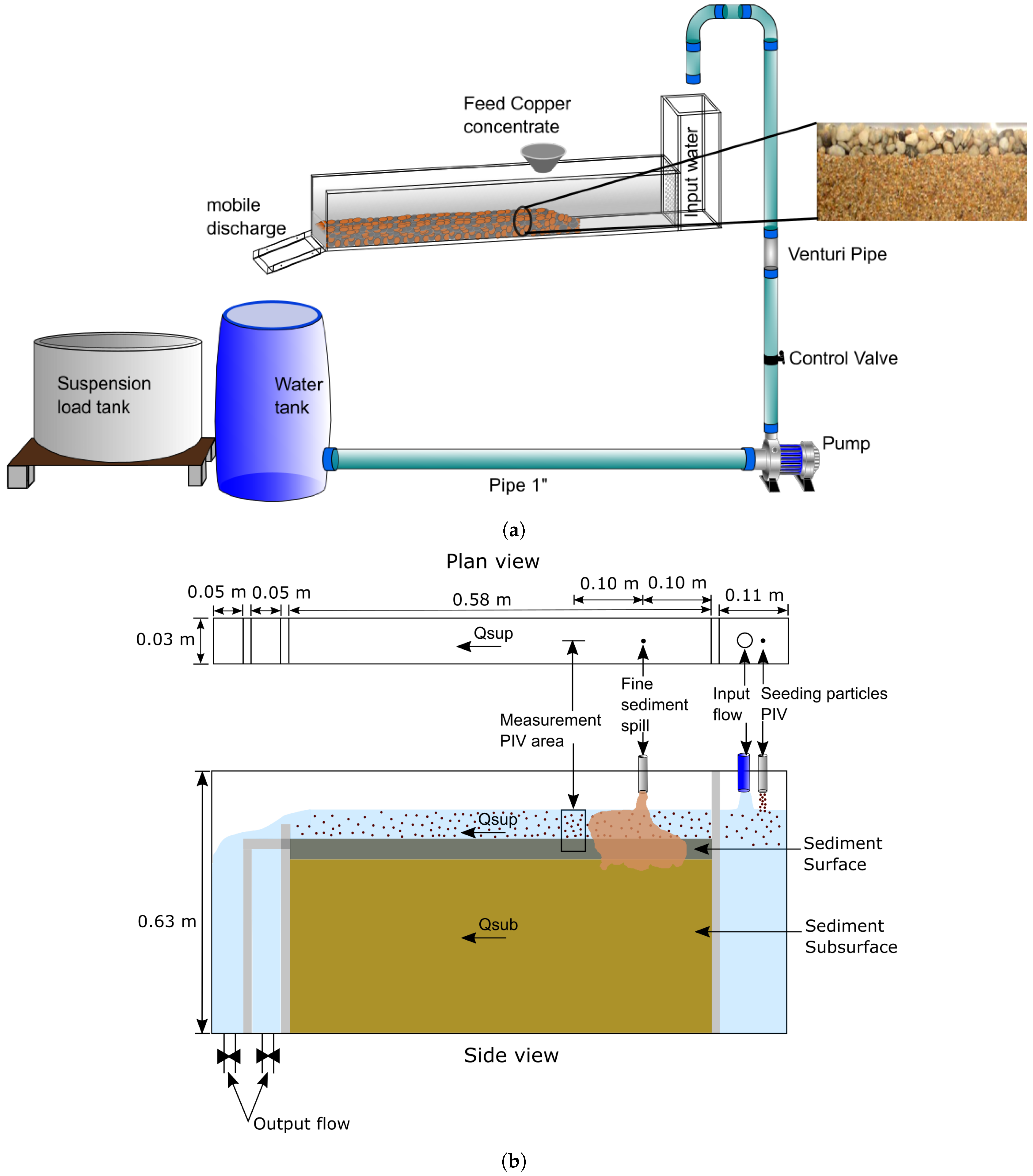
In this article, 10 experiments were carried out in a flume with 0.05 m of sediment substrate, named F1, and 24 experiments were carried out in a flume with 0.39 m of sediment substrate, named F2. The experiments in F1 were conducted in the experimental setup used by [25]. This setup consisted of an open channel 0.11 m wide, 3.0 m long, 0.15 m deep, and bed slope that varied between 0.007 and 0.047. The fine material was fed as punctual discharge through an acrylic cone, 2.83 cm in diameter. This system pours a flow rate of 0.23 l/s of copper concentrate for 7 s, and the net weight of fine sediment was $W_{spill}$ = 2.8 kg (Figure 1a).

The experiments in F2 were conducted in the experimental setup used by [29]. This setup consisted of an open channel, 0.03 m wide, 0.58 m long, and 0.63 m deep. The structure is divided into three sections. Upstream are the surface and subsurface input flows. At the center of the facility are the open channel, the bed, and the point where the fine material mixture is spilled. In the downstream area are the surface and subsurface output discharges. The fine material was fed through an acrylic cone in the free surface, of 1.0 cm of diameter, during 6 s. The net weight of fine material was between 0.070–0.284 kg for the experiments (Figure 1b). The flows in the experiments in both facilities are with fully developed turbulence. They have a relative depth, $H/D_g$, lower than 10, as observed in

Table 1. Sediment, mineral particles, and hydraulic parameters of flume, F1, and sediment column experiments, F2.

Exp	${\mathit{D}}_{50\mathit{s}}$	${\mathit{D}}_{50\mathit{c}}$	${\mathit{\sigma }}_{\mathit{gs}}$	${\mathit{\sigma }}_{\mathit{gc}}$	${\mathit{R}}_{\mathit{c}}$	${\mathit{Q}}_{\mathit{sur}}$	${\mathit{Q}}_{\mathit{sub}}$	H	$\mathit{H}/{\mathit{D}}_{\mathit{g}}$	A	${\mathit{U}}_{\mathit{sur}}$	${\mathit{U}}_{\mathit{sub}}$	${\mathit{R}}_{\mathit{h}}$	S	${\mathit{u}}_{\ast \mathit{th}}$	${{\mathit{Fr}}_{\mathit{d}}}^2$	${\mathit{Re}}_{\mathit{g}}$
#	m	m	-	-	-	l/s	l/s	m	-	m2	m/s	m/s	m	-	m/s	-	-
1-F1	0.0010	0.000040	1.34	2.22	3.2	0.61	0.000	0.030	2.0	0.003	0.185	0.000	0.019	0.047	0.890	0.11	1848
2-F1	0.0010	0.000040	1.34	2.22	3.2	0.61	0.000	0.030	2.0	0.003	0.185	0.000	0.019	0.047	0.900	0.11	1848
3-F1	0.0010	0.000040	1.34	2.22	3.2	0.61	0.000	0.030	2.0	0.003	0.185	0.000	0.019	0.047	0.890	0.11	1848
4-F1	0.0000	0.001360	1.23	2.25	3.2	1.95	0.000	0.030	2.0	0.003	0.591	0.000	0.019	0.047	0.089	1.11	5909
5-F1	0.0000	0.002120	1.44	2.13	3.2	1.95	0.000	0.043	2.9	0.005	0.412	0.000	0.024	0.047	0.103	0.54	4123
6-F1	0.0001	0.000940	1.26	1.85	3.2	1.82	0.000	0.057	3.8	0.006	0.290	0.000	0.028	0.003	0.043	0.27	2903
7-F1	0.0000	0.001360	1.23	2.52	3.2	1.82	0.18	0.057	3.8	0.006	0.290	0.055	0.028	0.003	0.043	0.27	2903
8-F1	0.0001	0.000940	1.26	2.01	3.2	2.45	0.24	0.067	4.5	0.007	0.332	0.073	0.030	0.003	0.044	0.35	3324
9-F1	0.0001	0.000940	1.26	2.87	3.2	2.30	0.23	0.063	4.2	0.007	0.332	0.070	0.029	0.003	0.044	0.35	3319
10-F1	0.0001	0.001360	1.23	2.12	3.2	2.50	0.25	0.053	3.5	0.006	0.429	0.076	0.027	0.036	0.064	0.59	4288
1-F2	0.0000	0.001290	1.38	3.04	3.2	0.00	0.00	0.019	1.3	0.001	0.000	0.000	0.008	0.000	0.000	0.00	0
2-F2	0.0001	0.001970	1.22	2.22	3.2	0.06	0.004	0.010	0.7	0.000	0.203	0.000	0.006	0.029	0.041	0.13	2033
3-F2	0.0001	0.001910	1.25	2.67	3.2	0.03	0.013	0.028	1.9	0.001	0.036	0.001	0.010	0.002	0.013	0.00	357
4-F2	0.0000	0.001870	1.24	2.20	3.2	0.07	0.006	0.033	2.2	0.001	0.067	0.001	0.010	0.004	0.019	0.01	667
5-F2	0.0000	0.001910	1.23	2.46	3.2	0.05	0.006	0.033	2.2	0.001	0.054	0.001	0.010	0.007	0.027	0.01	535
6-F2	0.0000	0.004430	1.25	2.35	3.2	0.10	0.004	0.026	1.7	0.001	0.132	0.000	0.010	0.005	0.022	0.06	1321
7-F2	0.0001	0.001970	1.22	2.31	3.2	0.06	0.046	0.031	2.1	0.001	0.061	0.004	0.010	0.007	0.027	0.01	613
8-F2	0.0001	0.001980	1.22	1.97	3.2	0.11	0.026	0.026	1.7	0.001	0.138	0.002	0.010	0.015	0.038	0.06	1385
9-F2	0.0000	0.001230	1.38	2.31	3.2	0.08	0.034	0.067	4.5	0.002	0.039	0.003	0.012	0.007	0.029	0.00	388
10-F2	0.0046	0.000044	1.46	1.79	3.2	0.11	0.035	0.057	3.8	0.002	0.064	0.003	0.012	0.017	0.045	0.00	388
11-F2	0.0000	0.004490	1.45	2.41	3.2	0.02	0.04	0.031	2.1	0.001	0.022	0.003	0.010	0.002	0.013	0.00	215
12-F2	0.0000	0.001760	1.03	2.57	3.2	0.13	0.053	0.056	3.7	0.002	0.077	0.005	0.012	0.003	0.020	0.02	774
13-F2	0.0001	0.001910	1.23	2.86	3.2	0.15	0.038	0.056	3.7	0.002	0.089	0.003	0.012	0.005	0.025	0.03	893
14-F2	0.0002	0.005700	1.49	1.63	3.2	0.16	0.033	0.049	3.3	0.001	0.109	0.003	0.011	0.002	0.014	0.04	1088
15-F2	0.0002	0.004640	1.46	1.51	0.7	0.08	0.004	0.050	3.3	0.002	0.051	0.000	0.012	0.004	0.020	0.04	507
16-F2	0.0001	0.005150	1.51	1.74	0.7	0.15	0.003	0.061	4.1	0.002	0.081	0.000	0.012	0.005	0.025	0.10	814
17-F2	0.0001	0.004840	1.47	1.73	0.7	0.06	0.043	0.048	3.2	0.001	0.042	0.004	0.011	0.002	0.014	0.03	424
18-F2	0.0001	0.002940	1.33	2.09	0.7	0.09	0.039	0.059	3.9	0.002	0.052	0.003	0.012	0.010	0.035	0.04	520
19-F2	0.0002	0.002830	1.55	1.76	0.5	0.12	0.036	0.058	3.9	0.002	0.069	0.003	0.012	0.010	0.035	0.10	690
20-F2	0.0002	0.002420	1.38	1.79	0.7	0.20	0.055	0.071	4.7	0.002	0.094	0.005	0.012	0.022	0.052	0.13	939
21-F2	0.0001	0.001950	1.24	1.98	0.7	0.11	0.005	0.070	4.7	0.002	0.052	0.000	0.012	0.014	0.041	0.04	524
22-F2	-	0.002800	1.20	-	0.7	0.14	0.033	0.055	3.7	0.002	0.085	0.003	0.012	0.022	0.051	0.10	848
23-F2	-	0.002720	1.28	-	0.7	0.15	0.038	0.066	4.4	0.002	0.076	0.003	0.012	0.023	0.052	0.08	758
24-F2	-	0.002590	1.37	-	0.7	0.09	0.08	0.067	4.5	0.002	0.044	0.001	0.012	0.017	0.045	0.03	438

, i.e., they are macroroughness flows, such as mountain rivers.

3.2. Materials and Instrumentation

An immobile bed of two layers of sediments, gravel and sands, was considered here, as did Bustamante-Penagos and Niño [25,29]. The gravel layer represents the active layer in gravel-bed rivers [13] and also prevents the transport of sand. Furthermore, the flow rate is low because the objective of this research is to analyze the phenomenon of static infiltration of fine material. That is, there is no bedload of the bed material. In both experiments, the sediment setup for an immobile bed was considered, with two layers of sediment. Gravel as the first layer, because the mineral particles can move freely through the interstitial spaces of the gravel (i.e., through an internal particle suspension, so there would always be unimpeded static percolation), and to analyze the bridging infiltration, a sublayer of sand was considered. The thickness of the gravel layer represents the active layer in natural rivers [30].

The surface layer was gravel, with 20 mm thickness, and has a mean diameter of $D_g=10$ mm, both in the F1 and F2 flumes. In the F1 flume, the subsurface layer was of sand or fine gravel. It has 30 mm thickness and has a mean diameter, $D_s$, variable between 0.2 and 3.35 mm in different experiments. In the F2 flume, the subsurface layer was sand or fine gravel. It has 390 mm thickness and mean diameters between 0.7 and 5.7 mm, for different runs (Figure 2). The density of both materials, gravel, and sand, was 2.65 g/cm³ and the porosity of the substrate is 0.4 ± 0.02 in the experiments.

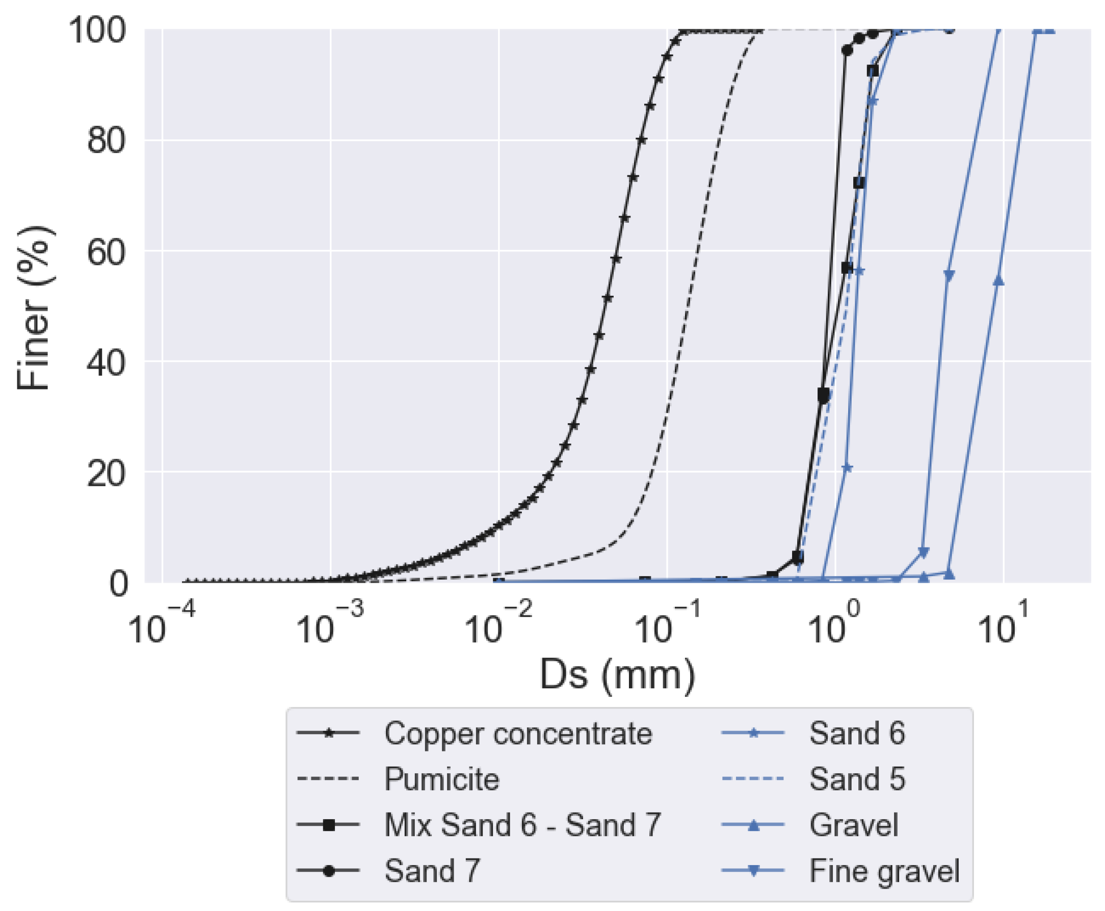
The fine sediments are copper concentrate, pumicite, and copper tailings. Only one experiment was made with actual copper tailings, but the pumicite recreates the clay-silt-sand content of tailings. The copper concentrate has a median diameter ($D_{50}$) of $D_c$ = 0.05 mm, a density of 4.2 g/cm${}^3$ and it is poured with a concentration of 56% by volume in water; the pumicite has a median diameter ($D_{50}$) of $D_c$ = 0.12 mm, a density of 1.7 g/cm${}^3$ and it is poured with a concentration of 77% by volume in water. Copper tailings have a median diameter $\left(D_{50}\right)$ of $D_c$ = 0.34 mm, a density of 1.5 g/cm${}^3$ and it is poured with a concentration of 56% by volume in water. Figure 2 reports the grain size distribution curves of gravel, fine gravel, three classes of sand (5, 6, or 7), copper concentrate, and pumicite. For each material, a different volumetric concentration was considered to avoid encapsulation, i.e., that it would only wet the particles.

The instrumentation used were a Venturi pipe for flow measurement, a Nikon D3200 camera for image analysis of fine sediment transport. The grain size distribution analysis of the fine particles is carried out in the Sedimentology Laboratory of the Universidad de Chile with Malvern Mastersizer 2000 equipment.

The experiments considered in this study are 34, 10 in F1, 24 in F2. Table 1 summarizes the mean diameters, $D_{50c}$, $D_{50s}$, and grain standard deviations, ${\sigma }_{gs}$, ${\sigma }_{gc}$, of the fine sediment and sands, hydraulic flow parameters; $Q_{sur}$, $Q_{sub}$, $U_{sur}$, $U_{sub}$, surface and subsurface flows and section mean velocities and H flow depth, A, wetted area; $R_h$, hydraulic radius, S, slope of the channel, $u_{th\ast }=\sqrt{gS{R}_h}$, theoretical bulk shear velocity, $R_c$, dimensionless submerged density of fine sediment, $F{r}_d^2$ = $U_{sur}^2/\sqrt{R_{s}g{D}_{50s}}$, densimetric Froude number squared of the bed particle and $R{e}_s=U_{sur}{D}_{50s}/\nu$, $R{e}_g=U_{sur}{D}_{50g}/\nu$, bed particle Reynolds number and gavel Reynolds number, respectively, with $\nu$ the kinematic viscosity.

On the other hand, each experimental data has an error associated with instrumental precision. The flow rate in F1 was measured through mass measurement with an accuracy scale of 0.1 kg and an accuracy of the Venturi pipe of 0.2 l/s, while the flow rate in F2 was measured through volumetric measurement with a 500 mL test tube and the accuracy was of 1 mL. For the geometrical parameters, flow depth, wetted area, and the infiltration depth of the copper concentrate, the error was by the pixel size, in this case it was 0.3 mm, whereas the error for infiltration depth of pumicite and tailings was 1 mm.

4. Results

4.1. Visualization of Infiltration of Fine Mineral Particles

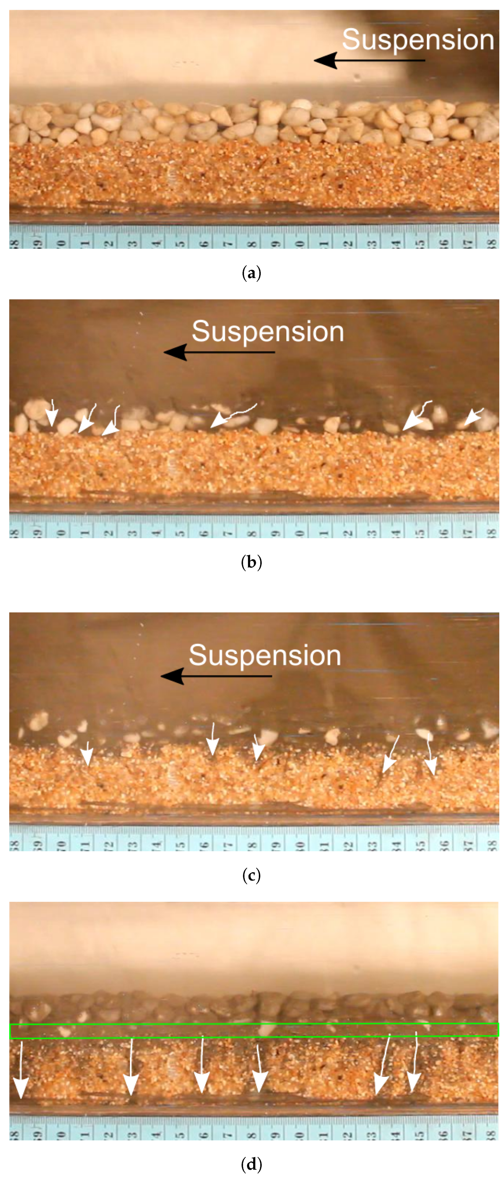
The transport dynamic of fine mineral particles, when poured as a hyper-concentrate mixture, begins with transport in suspension because the mixture enters the flow through the free surface. When the fine sediment is mixed throughout the water column, infiltration of fine material begins, first at the gravel layer and, later, into the substrate layer (sand or fine gravel). Figure 3 shows four characteristic instants of the dynamic of the fine sediment (experiment 7-F1, Table 1) in the water column and bed. In experimental setup F1, Figure 3a shows the suspended transport of the hyper-concentrated mixture of fine sediment, after mixing it in the water column. In Figure 3b, the white arrows show the infiltration of copper concentrate as it begins to move into the gravel layer. After that, infiltration of copper concentrate into the sand (or fine gravel) substrate is generated. Figure 3c shows that the infiltration of copper concentrate patterns look like fingers. Therein, the white arrows show the beginning of infiltration of copper concentrate into the sand substrate. Finally, the final state of unimpeded static percolation within the sand substrate is shown in Figure 3d. Finger patterns have been fully developed. In addition, the green box shows the largest zone of fine sediment accumulation. The accumulation zone is generated due to the vertical variation of pore size because there is a change from gravel to sand, and the pore size of the gravel is larger than the pore size of the sand.

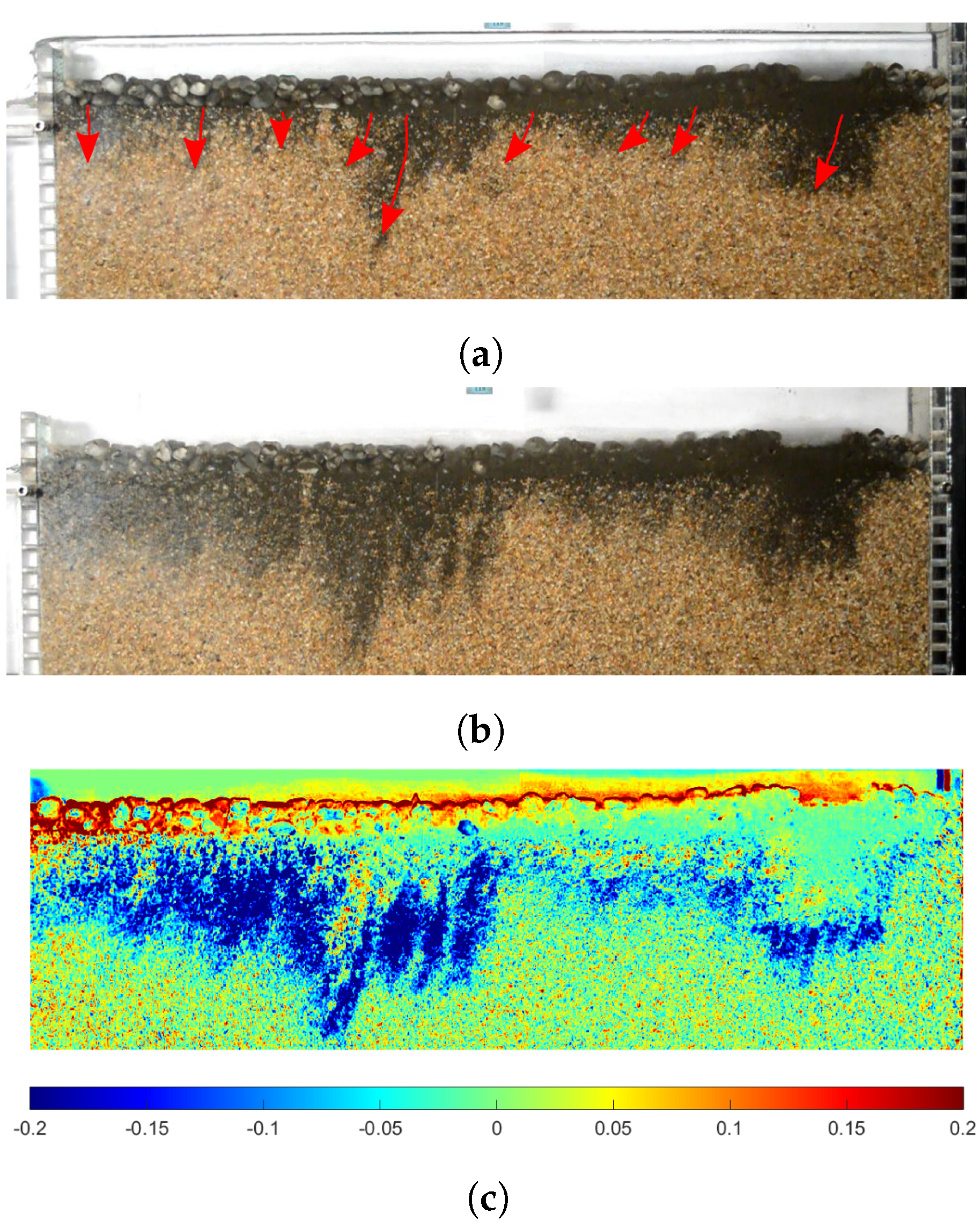
The infiltration of fine material analysis is also evaluated in experimental setup F2. In this case, the substrate height is 7.8 times larger than the substrate height size considered in F1. The maximum infiltration of fine material evaluated in F1 was for experiments with 30 mm sediment thickness and $d_s=$ 1.9 mm. So it is also evaluated in F2. However, bridging layer was found at greater depth than 30 mm and with an inclination associated with the subsurface flow. Figure 4 shows images of the experiment 5-F2. Figure 4a shows, with red arrows, the fingers patterns of the copper concentrate deposits and their inclination due to subsurface flow. When copper concentrate deposits reach a maximum, there is no movement in the substrate (Figure 4a). Nevertheless, when the input flow is cut off, like an ephemeral stream, the decrease in the surface water level increases the infiltration depth of fine sediment (Figure 4b), because, vertical variation of subsurface flow can destabilize the bridging. The increase of the infiltration depth of the copper concentrate was analyzed by image processing. This analysis considers the image in which the infiltration depth of copper concentrate reaches the steady-state (Figure 4a) and the image when the water level is minimum. So, Figure 4c is the result of subtracting Figure 4b of Figure 4a. Note that the dark blue tones in Figure 4c show the increase in infiltration to the maximum infiltration state of copper concentrate.

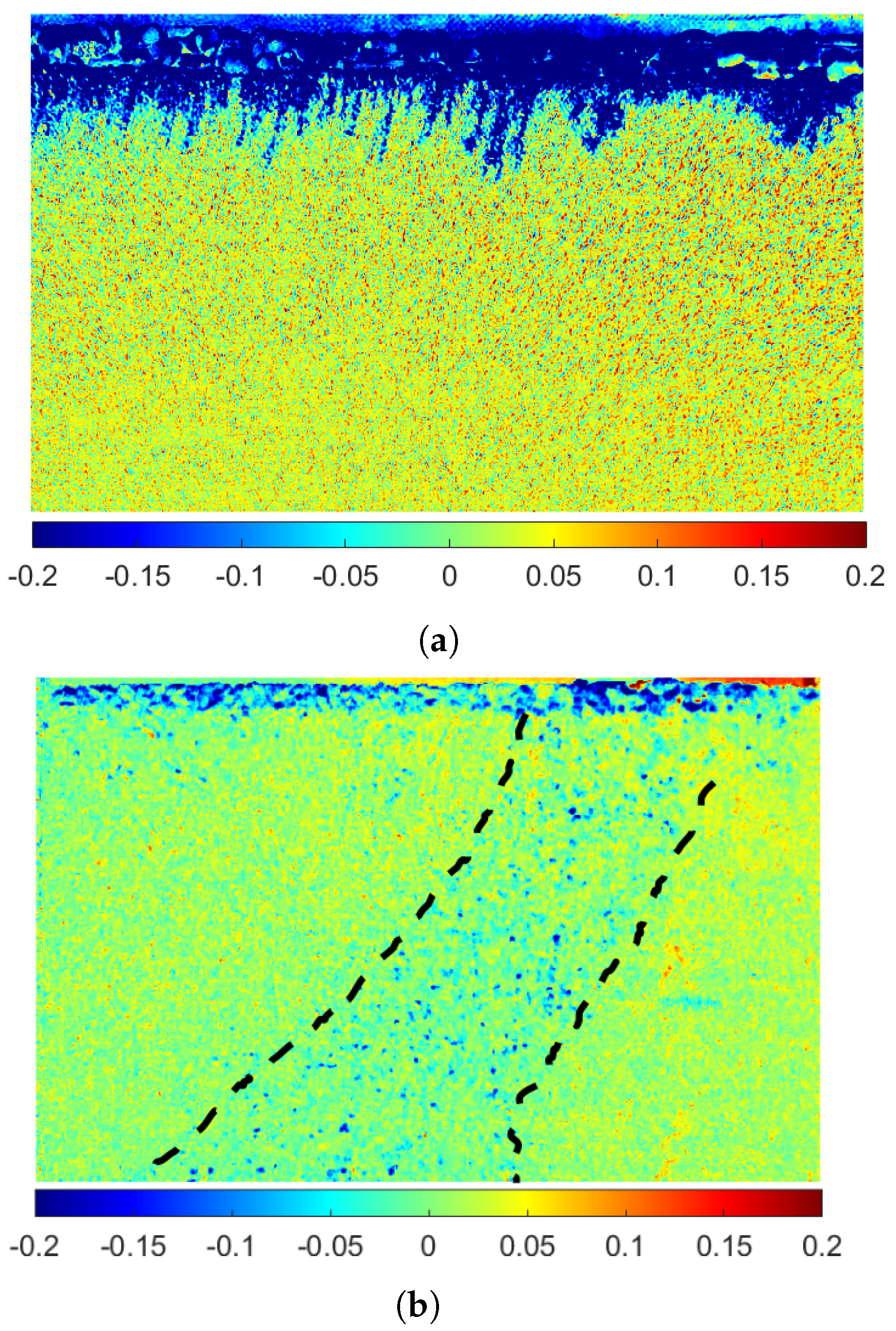
Sediment size greater than $D_s=$ 1.9 mm (fine gravel) was also considered in F2 to analyze the types of infiltration of fine materials. Both types of infiltration of fine materials, bridging, and unimpeded static percolation, were found. Figure 5 shows the bridging and unimpeded static percolation in F2. The color bar represents the concentration of copper concentrate in the sediment substrate sand (Figure 5a) and fine gravel (Figure 5b). The negative values in the color bar are because the intensities in an image are between 0–255. The zero intensity is associated with dark shades, while the 225 intensity is associated with light tones; i.e., when the infiltration of fine material increases its depth, the intensities decrease, so subtracting a final state from an initial state generates negative values when the analysis is performed with double format images. The dark blue shades are the deposition of copper concentrate, while red shades are the changes associated with a small reflection of acrylic and water. The dashed black lines in Figure 5b show the zone of copper concentrate infiltration into the substrate of fine gravel substrate. When the substrate is fine gravel, the copper concentrate deposition concentration is lower than when the substrate is sand because the substrate with large particles, gravel or cobbles, generates a larger storage area of fine material. Therefore, the fine particles can be redistributed over a larger area, and for this reason, the concentration of fine particles within the substrate decreases.

4.2. Hydraulic Parameters

Infiltration depth of fine material was analyzed according to the dimensionless parameters presented in Section 2. The $H/D_{50g}$ parameter was omitted because macro-roughness flows were present in both experimental setups. $H/D_{50g}$ was between 1.9 and 7.1, i.e., macro-roughness flows typical of mountains rivers, e.g., Aconcagua and Blanco rivers in Chile according to [8,31].

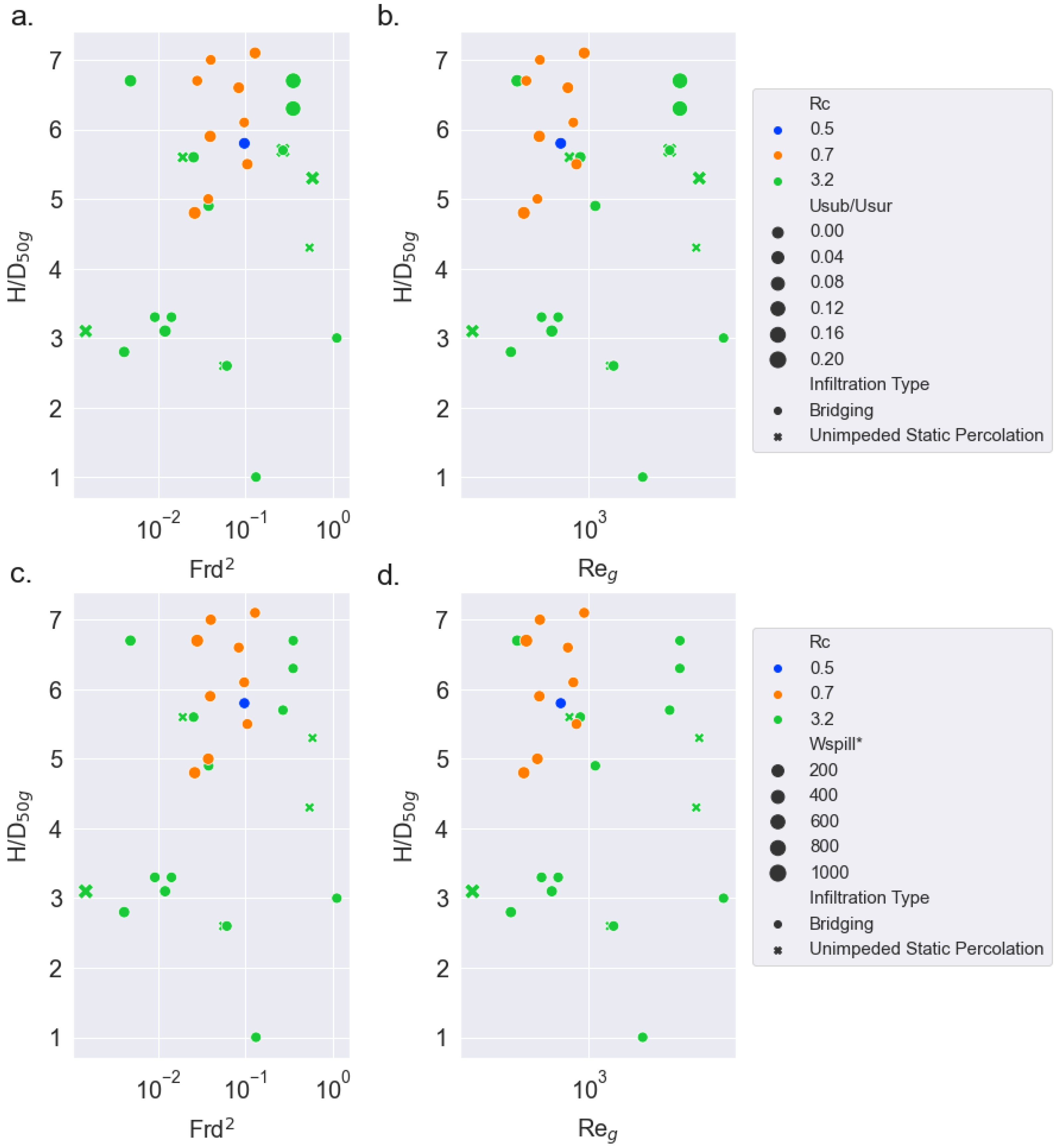
On the other side, the infiltration dimensionless depth and type and the hydraulic parameters such as $Fr{d}^2$ and $R{e}_g$ were analyzed considering the parameters $U_{sub}/U_{sur}$, $R_c$, $W_{spill}^{\ast }$. Figure 6a,b allows analyzing the relationship between infiltration dimensionless depth and type and $Fr{d}^2$ or $R{e}_g$, using $R_c$, and $U_{sub}/U_{sur}$ as secondary parameters. Figure 6c,d allows analyzing the same relationship but using $R_c$, and $W_{spill\ast }$ as secondary parameters. However, we did not find a relationship between the infiltration dimensionless depth and type and $Fr{d}^2$ or $R{e}_g$, i.e., pollution into the bed is independent of hydraulic parameters, as [14,25,27,28] reported.

4.3. Infiltration Depth of Fine Mineral Particles

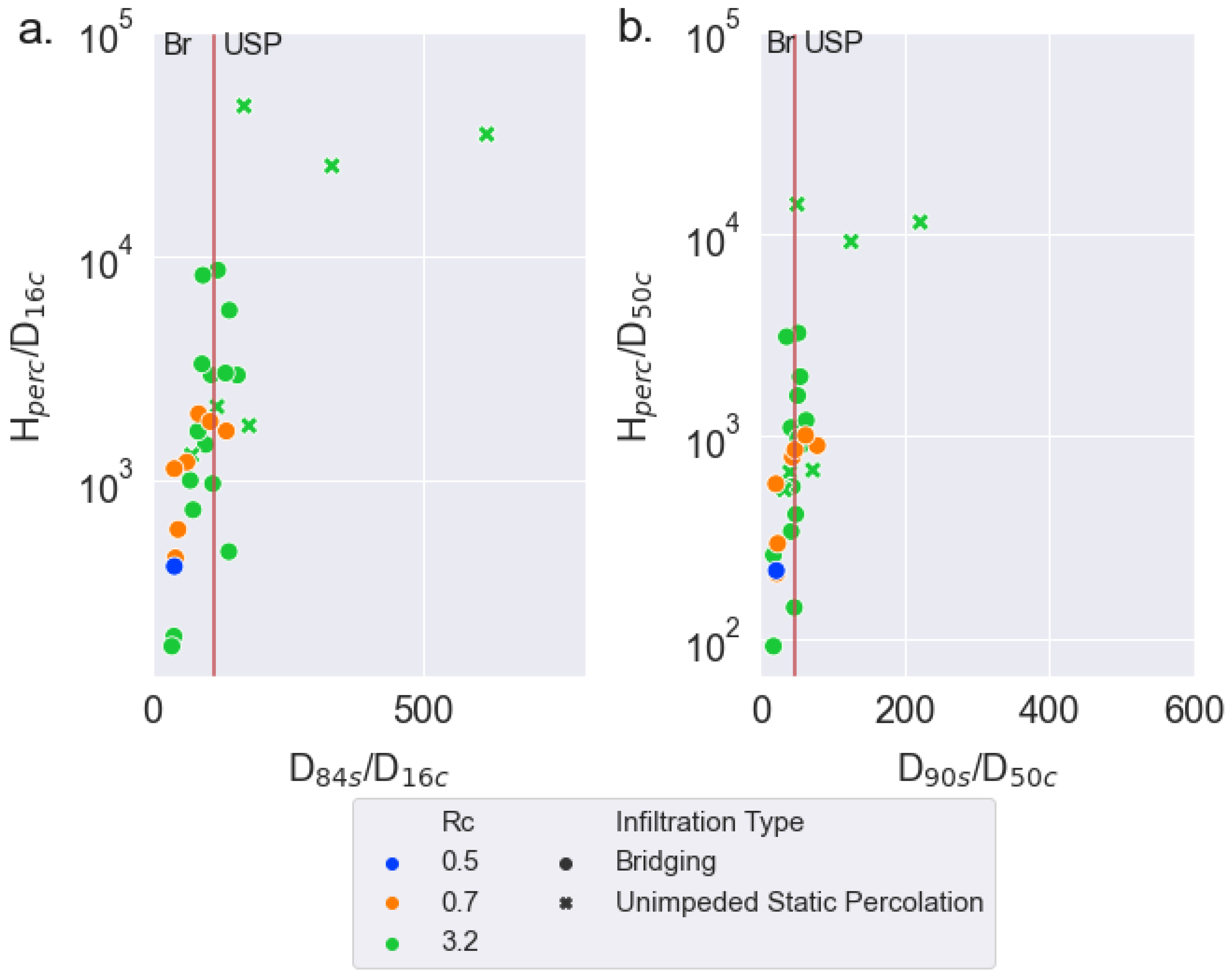
The infiltration depth for copper concentrate, pumicite, and tailings was analyzed considering hydraulic parameters do not effect infiltration depth, according to the analysis presented in Section 4.2. The geometric relationships considered were $D_{50s}/D_{50c},$$D_{84s}/D_{16c}$ and $D_{90s}/D_{50c}$. These relationships were considered by [25] as good candidates to characterize the maximum infiltration type of copper concentrate in gravel beds. Figure 7 shows the thresholds corresponding to red lines proposed by [25] characterizing bridging or unimpeded static percolation. The colors represent each of the fine particles and the marker shows the infiltration type. Therefore, we can see that none of the thresholds, $D_{84s}/D_{16c}>115$ and $D_{90s}/D_{50c}>47$, adequately characterize the infiltration type. The infiltration reported as unimpeded static percolation in F1 was seen as a bridging layer in F2. For this reason, we propose that the concept of unimpeded static percolation is relative to the depth of the substrate, and this concept should be reevaluated to characterize the type of infiltration of fine materials. Unimpeded static percolation could become a bridging in a thicker substrate. We were able to find that the unimpeded static percolation reported by [25] became bridging in a thicker substrate. Under this argument, we postulate that the type of infiltration of fine material is relative to the depth of the substrate and the change in soil properties at depth.

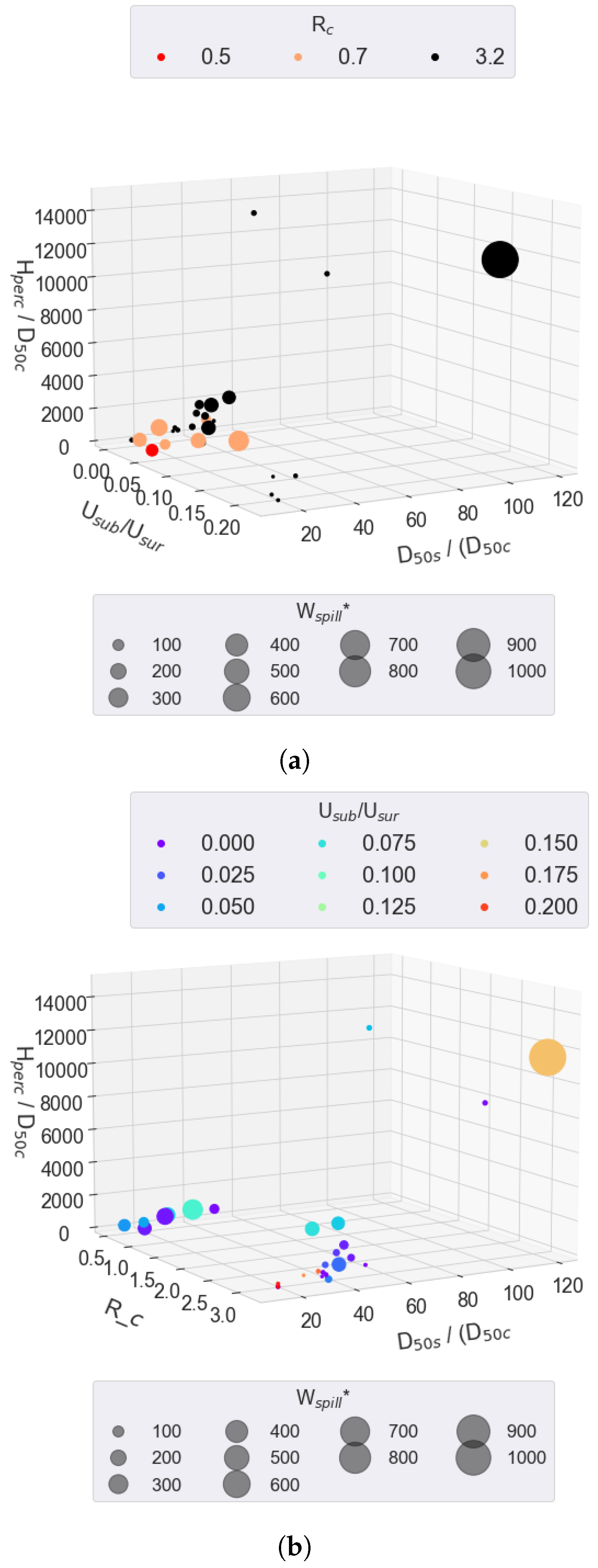
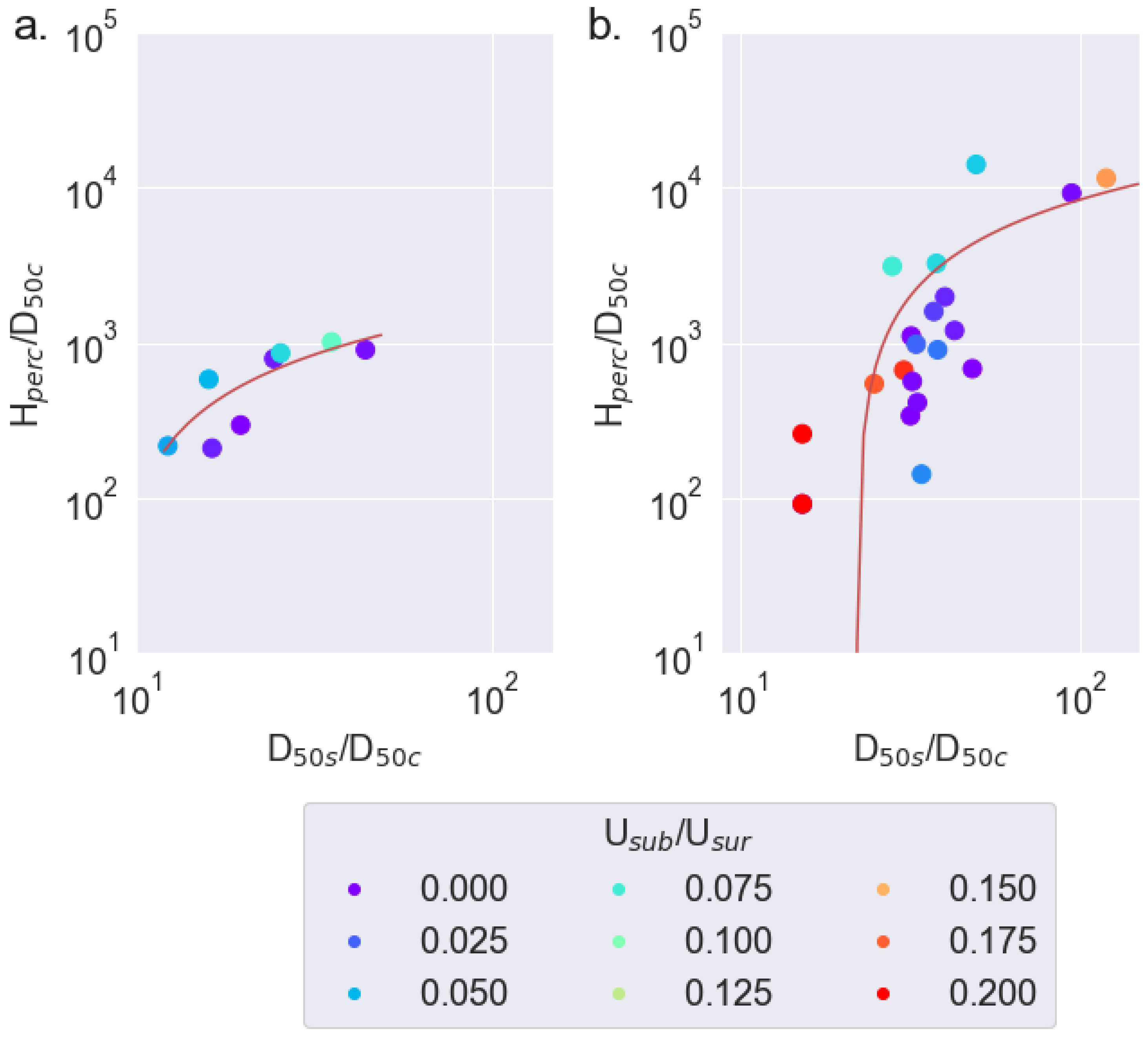
On the other hand, the dimensionless ratio of the maximum infiltration depth was analyzed by considering both $U_{sub}/U_{sur}$, and $D_{50s}/D_{50c}$ (Figure 8a). $R_c$ is represented by the color of the experimental points, and $W_{spill}\ast$ is represented by the size of the experimental points. Whereas Figure 8b considers the dimensionless ratio of the maximum infiltration depth as a function of $R_c$, and $D_{50s}/D_{50c}$. In this case, the color of the experimental points represents $U_{sub}/U_{sur}$, and the size of the experimental points represents $W_{spill}\ast$. Figure 8 shows that $H_{perc}/D_{50c}$ increase with $D_{50s}/D_{50c}$, and is independent of $W_{spill}\ast$. The independence between $H_{perc}/D_{50c}$ and $W_{spill}\ast$ implies that the depth of contaminated substrate after a mining accident is independent of the magnitude of the fine material dumped. The highest contamination will be in the first few centimeters of the substrate. Of course, the bigger is the accident, the more area of the river bed is affected.

Furthermore, Figure 8b shows that the dimensionless submerged density is the key parameter for analyzing the infiltration of fine material phenomenon. Note that, $R_c\sim$ 0.5–0.7 has lower variability than that associated with $R_c\sim$ 3 for different $D_{50s}/D_{50c}$. The dimensionless relationship of the maximum infiltration depth is analyzed as a function of only $D_{50s}/D_{50c}$, considering $R_c\sim$ 0.5–0.7 separated from and $R_c\sim$ 3. Figure 9 shows the experimental data and the trend lines of adjustment (red lines). Figure 9a corresponds to $R_c\sim$ 0.5–0.7 and Figure 9b corresponds to $R_c\sim$ 3. The logarithmic functions to characterize the dimensionless relationship of the maximum infiltration depth $H_{perc}/D_{50c}$ as a function of $D_{50s}/D_{50c}$ are reported in Equation (3). In addition, the metrics of trend lines of the Equation (3), such as the coefficient of determination $r^2$, and the root mean square error, RMSE, are for $R_c\sim$ 0.5–0.7, $r^2$ = 0.73 and RMSE = 159.73. Whereas for $R_c\sim$ 3, $r^2$ = 0.49, RMSE = 2758.31.

$$\frac{H_{perc}}{D_{50c}}=\left\{\begin{array}{c}\hfill 655.2ln\left(0.11\frac{D_{50s}}{D_{50c}}\right)R_c\sim 0.5-0.7\\ \hfill 5493.9ln\left(0.05\frac{D_{50s}}{D_{50c}}\right)R_c\sim 3.2\end{array}\right.$$

(3)

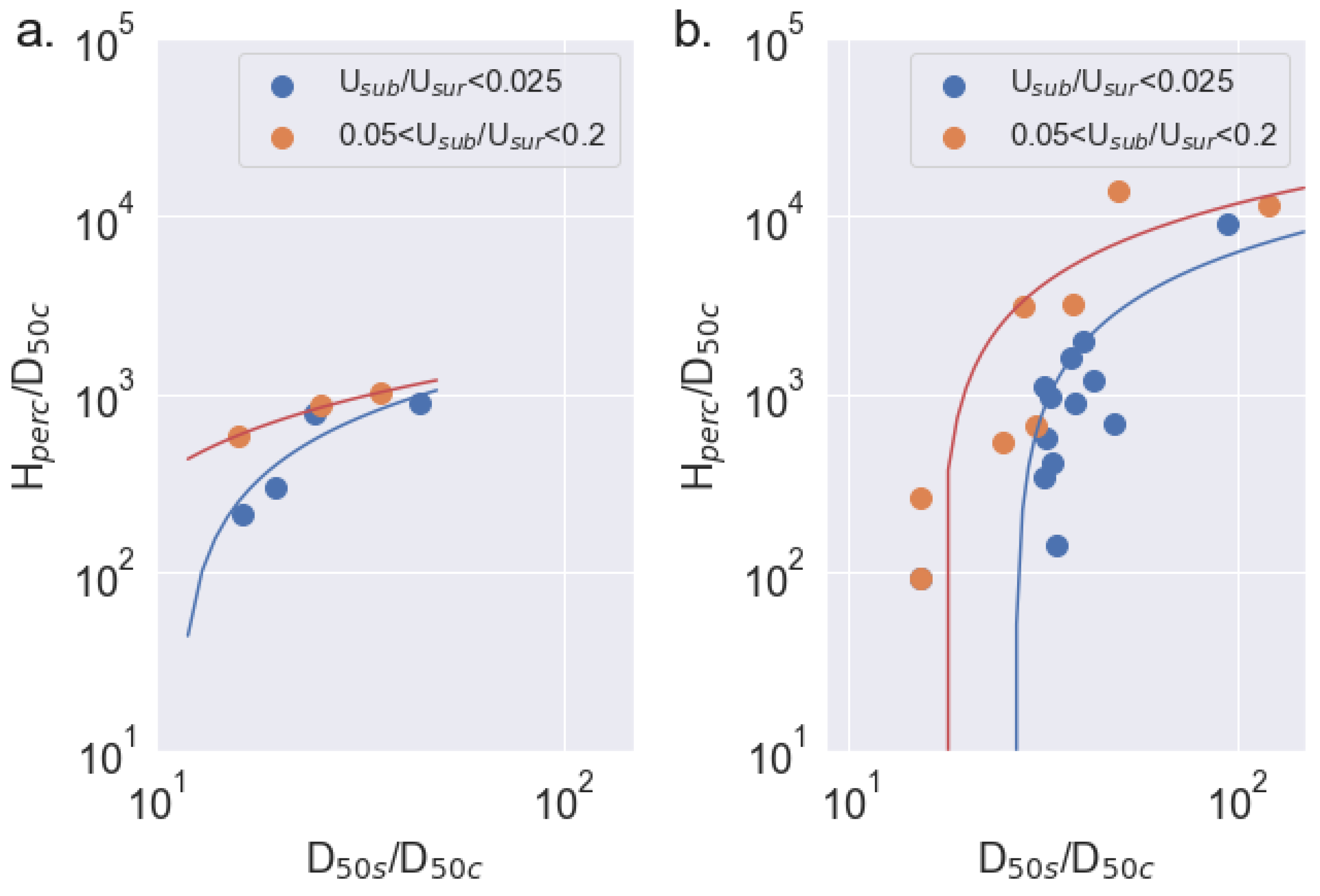
According to Figure 9, we can report an effect of the velocity ratio, $U_{sub}/U_{sur}$, and $R_c$ in the maximum dimensionless infiltration depth. However, statistical metrics such as $r^2$ and RMSE indicate that the relationship is weak, so we complement the analysis by considering two scales for the velocity ratio, $U_{sub}/U_{sur}<0.025$ and $0.05<U_{sub}/U_{sur}<0.2$ (Figure 10). So, the maximum dimensionless infiltration depth as function of $D_{50s}/D_{50c}$, $U_{sub}/U_{sur}$ and $R_c$ are defined by Equation (4), with their statistical metrics, $r^2$ and RMSE. Note that the statistical metrics shows a better correlation between the maximum dimensionless infiltration depth, the ratio of diameters of particles and velocity ratio. Therefore, we can consider an equation of the type $H_{perc}/D_{50c}=Aln(B{D}_{50s}/D_{50c})$ where A and B might be functions of $U_{sub}/U_{sur}$. However, more experiments are needed to determine the relationship between the coefficients A, B with $U_{sub}/U_{sur}$.

$$\frac{H_{perc}}{D_{50c}}=\left\{\begin{array}{c}\hfill 716.08ln\left(0.09\frac{D_{50s}}{D_{50c}}\right)R_c\sim 0.5--0.7\&U_{sub}/U_{sur}<0.025;r^2=0.79;RMSE=138\\ \hfill 544.09ln\left(0.18\frac{D_{50s}}{D_{50c}}\right)R_c\sim 0.5--0.7\&0.05<U_{sub}/U_{sur}<0.20;r^2=0.99;RMSE=12\\ \hfill 4752.53ln\left(0.04\frac{D_{50s}}{D_{50c}}\right)R_c\sim 3.0\&U_{sub}/U_{sur}<0.025:r^2=0.62;RMSE=1409\\ \hfill 6647.66ln\left(0.06\frac{D_{50s}}{D_{50c}}\right)R_c\sim 3.0\&0.05<U_{sub}/U_{sur}<0.20;r^2=0.67;RMSE=2966\end{array}\right.$$

(4)

5. Discussion

5.1. Scale Effects

The fine materials used in this research are highly polluting and toxic, so small flumes were considered to avoid high contamination of wastewater. Moreover, the acquisition of granulometric data took approximately a week because it was necessary to sieve the bed, both for the sands and for the fine material, and remove the fine material from the experiments and put them in separate barrels for their disposal. All that made the experiments as small-scale as possible. In addition, researchers such as [14,25,32], reported that the infiltration phenomenon is independent of the hydraulic parameters, so narrow flumes could be considered.

In both facilities, F1 and F2, the ratio $B/H<5$, so there is a wall effect and the dip phenomenon is present, i.e., the maximum velocities appear below the surface water [33], and the Vanoni correction is necessary to process the velocity field measurements and the bed shear stress [34].

On the other hand, according to [14,25,32], as the infiltration phenomenon is independent of the surface hydraulic parameters, the F1 and F2 have a width of 0.11 m and 0.03 m, respectively, and substrates with a thickness of 30 mm 390 mm. The narrowest flume F2 made it possible to analyze the infiltration depth and subsurface flow simultaneously. Ten experiments were run in F1 and 24 in F2. The 30 mm thick substrate of F1 is sometimes too small to analyze bridging and unimpeded static percolation as infiltration types. F2 allows for an analysis of the infiltration type, considering a larger substrate size. For instance, in F1 unimpeded static percolation was found for very coarse sand. However, in F2, bridging infiltration was found with the same sand. The flows in the experiments in both facilities are with fully developed turbulence. They have a relative depth, $H/D_g$, lower than 10, as observed in Table 1, i.e., they are macro-roughness flows, such as mountain rivers, and the flow resistance changes regarding the simple rough flow [21,31,35,36]. In the experiments, the spilled mixture was in the center of the cross-section, and the length of the complete mixing, l, in the cross-section was reached at $l\sim$ 0.70 m and $l\sim$ 0.17 m for F1 and F2, respectively. The mixing length in F1 and F2 were estimated considering the experimental data reported by [25,29], respectively. The ratio $l/B$ is 6.6 and 5.8, for F1 and F2, respectively, while in rivers highly polluted by mining accidents such as the Blanco River, in Chile, the complete mixing in the cross-section was reached at $l/B\sim$ 5.0. Therefore, we can analyze the suspension dynamics of the spill of copper concentrate in the F1 and F2 experiments, because the experimental setup can represent the natural conditions of gravel-rivers. The experimental setup F2 can allow us to analyze the substrate dynamic of the phenomenon of infiltration of fine material in the substrate, more than the experiments with F1, because it has a thicker substrate.

5.2. Visualization of Infiltration of Fine Mineral Particles

Infiltration of fine sediments in gravel beds has shown different infiltration patterns, depending on the type of sediment considered as contaminant material. Researchers such as [14,15,21] reported depositions from the bottom of the bed to the top of the gravel layer. In these studies, fine sediment fed the system at a constant rate. However, the infiltration pattern changes when the fine sediment feed is a point discharge of a hyper-concentrated mixture of fine sediment and water, as in the present research. On the other hand, when a gravel bed is contaminated with sands, ref. [21] reported a transport of sands within the gravel bed. However, when the contaminating sediment is a cohesive sediment, such as copper concentrate, tailings, or pumicite, this dynamic was not observed. On the contrary, once the copper concentrate is deposited on the substrate, it is only transported vertically when there is a decrease in the phreatic level. Fingers could have an inclination that depends on the depth of the substrate. Substrates with small depth imply vertical fingers without inclination. Conversely, deep substrates imply that the fingers will have an inclination associated with the subsurface flows. Additionally, considering a substrate like the ones we have in this article, we also found that copper concentrate infiltration can be up to 10 times greater than tailings or pumicite.

5.3. Infiltration of Fine Sediment

River pollution associated with the infiltration of fine sediments into the substrate has a high environmental impact because fine sediments can modify the interaction between surface and subsurface flows [10,12,14,15,16,17]. Furthermore, when the fine materials are heavy metals or mineral particles that come from mining activities, the contamination is more critical because these materials are toxic and could reside for a long time in the substrate [6]. For example, in Chile, mining companies process copper material as a sulfide ore. It has a characteristic diameter ($D_{50}$) $D_c$ = 40 $\mathsf{\mu }$m, a density of 4.2 g/cm${}^3$ and approximately between 30 and 40% is copper and the rest are 24–26% iron, 24–27% sulfur, 2.5–3.0% aluminum, 0.03% arsenic and other components.

The infiltration depth of fine material has not shown a relationship between flow parameters, and the amount of fine sediment spilled. This behavior has been reported both in this research and by researches such as [14,25,27]. Conversely, the geometric relationship between diameters has allowed characterizing the type of infiltration of fine material. However, there is no single threshold to characterize the infiltration phenomenon of fine material. Refs. [14,25,27,28,37] reported unimpeded static percolation and bridging as types of infiltration of fine material, although we think that the unimpeded static percolation as a concept should be re-evaluated. The thickness of the substrate becomes key to define the type of infiltration of fine material. For example, we found bridging layers in F2, but in F1 we found unimpeded static percolation. Therefore, the unimpeded static percolation can become bridging in a deeper substrate. At least, with the results shown in this article, particles of tailings ($R_c\sim$ 0.5–0.7) have no unimpeded static percolation and instead have a bounded bridging value.

The infiltration and deposition of fine mineral particles decrease in depth. That infiltration of fine material dynamics have also been reported in both experimental and field investigations according to [15,16,24,25,27], i.e., the decrease in depth deposition has also been validated with natural and non-natural sediments, such as copper concentrate and tailings. This behavior of fine sediment deposition shows that after a mining accident, most of the contaminated material is located in the first layer of riverbed sediments and this is independent of the magnitude of the mining accident.

Figure 9 shows that the logarithmic functions characterize the maximum dimensionless infiltration depth of fine material as a function of $D_{50s}/D_{50c}$ and $R_c$; the coefficients of determination, r${}^2$, are 0.73 for $R_c\sim$ 0.5–0.7 and 0.49 for $R_c\sim$ 3. Meanwhile, the coefficients of determination increase up to 28% when both $D_{50s}/D_{50c}$ and $U_{sub}/U_{sur}$ are considered in the analysis. So, this analysis shows that the parameters $R_c$, $D_{50s}/D_{50c}$, and $U_{sub}/U_{sur}$ influence the infiltration phenomenon of fine material, but $R_c$ was shown to be key to characterize the infiltration phenomenon of fine material. $R_c$ can generate higher infiltrations of fine material, while the $U_{sub}/U_{sur}$ parameter showed only a weak effect.

In Figure 10, for $R_c\sim$ 0.5–0.7, it is seen that the maximum values for the maximum dimensionless infiltration of fine material reach more or less 1.5 × 10${}^3$, when extrapolating the trends indicated there for the values of $D_{50s}/D_{50c}\sim$ 100. On the other hand, in Figure 10b, for $R_c\sim$ 3, the maximum values for the maximum dimensionless infiltration of fine material reach values over 10${}^4$, for the values of $D_{50s}/D_{50c}\sim$ 100. That is, the copper concentrate reaches values of the maximum dimensionless infiltration that are of the order of 10 times that of the pumacite or the tailings.

As reported in the introduction, mining accidents are highly polluting and the residence time in the bed is prolonged. Nevertheless, this article shows that once the fine mining particles infiltrate the bed, there is no bedload transport of contaminant materials. However, fine material can be resuspended during periods of high flows or snowmelt. Therefore, the effect of a mining accident will have long-term effects. According to [8], near the mines in the Aconcagua river basin, the Aconcagua River and its tributaries have a high sediment transport capacity, which decreases along the river. Namely, the reincorporation of fine material to suspension transport is high in the upper part of the basin and low in the area near the mouth of the Aconcagua River to the Pacific Ocean. On the other hand, Byrne [6] reported that copper may be transported due to seasonal oxidation of fine material or high flows associated with snowmelt and precipitation. So, in the lower part of the Aconcagua river basin, or any mountain river affected by mining activity, for that matter, the entrainment of heavy metals to the surface flow is also associated with the oxidation of heavy metals deposited in the substrate.

In addition, we found that the depth of infiltration of fine material could increase due to the decrease in surface and subsurface flows. This behavior will be typical of ephemeral streams that are being affected by climate change.

6. Conclusions

We have analyzed the infiltration of fine mineral particles in the bed of a gravel river, considering the hydraulic parameters of the flow, the mineral particles sizes, the amount of feed material, the density of the fine contaminant material, and the surface and subsurface flows. It was found that neither the amount of fine material dumped nor the hydraulic parameters of the surface flow affect the infiltration depth of fine material. On the other hand, an increase in the contamination of the substrate was found due to a decreasing phreatic level. This behavior could be found in ephemeral streams. It was also found that most of the fine contaminant material is retained in the first few centimeters of the substrate and decreases with depth. Therefore, it was found that the infiltration depth of fine material is independent of the magnitude of the mining accident and the surface layer or active layer of the riverbed is the one that retains most of the contaminating material. The maximum values obtained in this research for the maximum infiltration of tailings particles ($R_c\sim$ 0.5–0.7) seem to be close to 1000 $D_{50c}$ and are expected to have no unimpeded static percolation and instead have a bounded bridging value. The copper concentrate reaches values of the maximum dimensionless infiltration that are of the order of 10 times that of the pumacite or the tailings. Furthermore, it was also found that the concept of unimpeded static percolation should be reevaluated since it was found that the type of infiltration of fine material is relative to the depth of the substrate.

Logarithmic functions characterize the maximum dimensionless infiltration depth as a function of $D_{50s}/D_{50c}$ and $R_c$. The coefficients of determination increase up to 28% when both $D_{50s}/D_{50c}$ and $U_{sub}/U_{sur}$ are considered in the analysis. Therefore, this analysis shows that while the parameters $R_c$ and $U_{sub}/U_{sur}$ have an influence on the infiltration phenomenon, $R_c$ was shown to be the key to characterizing the infiltration phenomenon. $R_c$ can generate higher infiltrations of fine material, while the parameter $U_{sub}/U_{sur}$ shows only a weak effect.

Finally, we found that the coefficients of the logarithmic function are a function of the velocity ratio, $U_{sub}/U_{sur}$. As future work, more experiments that vary the velocity ratio are needed to determine with greater certainty how these coefficients are related to the coefficients with $U_{sub}/U_{sur}$ parameters.

References

- Coulthard, T.J.; Macklin, M.G. Modeling long-term contamination in river systems from historical metal mining. Geology 2003, 31, 451–454. [Google Scholar] [CrossRef]
- Macklin, M.G.; Brewer, P.A.; Hudson-Edwards, K.A.; Bird, G.; Coulthard, T.J.; Dennis, I.A.; Lechler, P.J.; Miller, J.R.; Turner, J.N. A geomorphological approach to the management of rivers contaminated by metal mining. Geomorphology 2006, 79, 423–447. [Google Scholar] [CrossRef]
- Byrne, P.; Hudson-Edwards, K.; Macklin, M.; Brewer, P.; Bird, G. The long-term environmental impacts of the Mount Polley mine tailings spill, British Columbia, Canada. Geophys. Res. Abstr. 2015, 17, 6241. [Google Scholar]
- Jaskuła, J.; Sojka, M.; Fiedler, M.; Wróżyński, R. Analysis of spatial variability of river bottom sediment pollution with heavy metals and assessment of potential ecological hazard for the Warta river, Poland. Minerals 2021, 11, 327. [Google Scholar] [CrossRef]
- Benito, G.; Benito-Calvo, A.; Gallart, F.; Martín-Vide, J.P.; Regües, D.; Bladé, E. Hydrological and geomorphological criteria to evaluate the dispersion risk of waste sludge generated by the Aznalcollar mine spill (SW Spain). Environ. Geol. 2001, 40, 417–428. [Google Scholar] [CrossRef]
- Byrne, P.; Hudson-Edwards, K.A.; Bird, G.; Macklin, M.G.; Brewer, P.A.; Williams, R.D.; Jamieson, H.E. Water quality impacts and river system recovery following the 2014 Mount Polley mine tailings dam spill, British Columbia, Canada. Appl. Geochem. 2018, 91, 64–74. [Google Scholar] [CrossRef]
- Do Carmo, F.F.; Kamino, L.H.Y.; Junior, R.T.; de Campos, I.C.; do Carmo, F.F.; Silvino, G.; Mauro, M.L.; Rodrigues, N.U.A.; Miranda, M.P.d.S.; Pinto, C.E.F. Fundão tailings dam failures: The environment tragedy of the largest technological disaster of Brazilian mining in global context. Perspect. Ecol. Conserv. 2017, 15, 145–151. [Google Scholar] [CrossRef]
- CENMA. Analysis of the Physical-Chemical Composition of River Sediments and Their Relationship with the Availability of Metals in Water in the Aconcagua River Basin; Technical Report; Centro Nacional del Medio Ambiente, Universidad de Chile: Santiago, Chile, 2008. [Google Scholar]
- Soublette, N.; Heyer, A.; Cortes, I. Preliminary and Confirmatory Investigation of Soils with Potential Presence of Contaminants (SPPC); Technical Report; National Environment Center: Illapel, Chile, 2011. (In Spanish) [Google Scholar]
- Tonina, D.; Buffington, J.M. Hyporheic Exchange in Mountain Rivers I: Mechanics and Environmental Effects. Geogr. Compass 2009, 3, 1063–1086. [Google Scholar] [CrossRef]
- Mcdowell-Boyer, L.M.; Hunt, J.R.; Sitar, N. Particle Transport Through Porous Media. Water Resour. Res. 1986, 22, 1901–1921. [Google Scholar] [CrossRef]
- Findlay, S. Importance of surface-subsurface exchange in stream ecosystems: The hyporheic zone. Limnol. Oceanogr. 1995, 40, 159–164. [Google Scholar] [CrossRef]
- Cui, Y.; Parker, G. The arrested gravel front: Stable gravel-sand transitions in rivers Part 2: General numerical solution. J. Hydraul. Res. 1998, 36, 159–182. [Google Scholar] [CrossRef]
- Beschta, R.; Jackson, W. The Intrusion of Fine Sediments into a Stable Gravel Bed. J. Fish. Res. Board Can. 1979, 36, 204–210. [Google Scholar] [CrossRef]
- Diplas, P.; Parker, G. Pollution of Gravel Spawning Grounds due to Fine Sediment; Technical Report 240; Unversity of Minnesota: Minneapolis, MN, USA, 1985. [Google Scholar]
- Lisle, E. Sediment Transport and Resulting Deposition in Spawning Gravels, North Coastal California. Water Resour. Res. 1989, 25, 1303–1319. [Google Scholar] [CrossRef] [Green Version]
- Shrivastava, S. Influence of Bioturbation and Fine Sediment Clogging on Hyporheic Exchange in Streams. Ph.D. Thesis, The University of Melbourne, Melbourne, Australia, 2020. [Google Scholar]
- Fox, J.F.; Asce, M. Prediction of the Clogging Profile Using the Apparent Porosity and Momentum Impulse. J. Hydraul. Eng. 2016, 142, 06016016. [Google Scholar] [CrossRef]
- Sambrook Smith, G.H.; Nicholas, A.P.; Ferguson, R.I. Measuring and defining bimodal sediments: Problems and implications. Water Resour. Res. 1997, 33, 1179–1185. [Google Scholar] [CrossRef]
- Sambrook Smith, G.H.; Nicholas, A.P. Effect on flow structure of sand deposition on a gravel bed: Results from a two-dimensional flume experiment. Water Resour. Res. 2005, 41, 1–12. [Google Scholar] [CrossRef] [Green Version]
- Niño, Y.; Licanqueo, W.; Janampa, C.; Tamburrino, A. Front of unimpeded infiltrated sand moving as sediment transport through immobile coarse gravel. J. Hydraul. Res. 2018, 56, 697–713. [Google Scholar] [CrossRef]
- Edroma, E.L. Copper Pollution in Rwenzori National Park, Uganda. J. Appl. Ecol. 1974, 11, 1043–1056. [Google Scholar] [CrossRef]
- Cui, Y.; Wooster, J.K.; Baker, P.F.; Dusterhoff, S.R.; Sklar, L.S.; Dietrich, W.E. Theory of fine sediment infiltration into immobile gravel bed. J. Hydraul. Eng. 2008, 134, 1421–1429. [Google Scholar] [CrossRef] [Green Version]
- Wooster, J.K.; Dusterhoff, S.R.; Cui, Y.; Sklar, L.S.; Dietrich, W.E.; Malko, M. Sediment supply and relative size distribution effects on fine sediment infiltration into immobile gravels. Water Resour. Res. 2008, 44, 1–18. [Google Scholar] [CrossRef] [Green Version]
- Bustamante-Penagos, N.; Niño, Y. Suspension and infiltration of copper concentrate in a gravel bed: A flume study to evaluate the fate of a potential spill in a Chilean river. Environ. Earth Sci. 2020, 79, 530. [Google Scholar] [CrossRef]
- Iseya, F.; Ikeda, H. Pulsations in bedload transport rates induced by a longitudinal sediment sorting: A flume study using sand and gravel mixtures. Geogr. Ann. Ser. Phys. Geogr. 1987, 69, 15–27. [Google Scholar] [CrossRef]
- Gibson, S.; Abraham, D.; Heath, R.; Schoellhamer, D. Vertical gradational variability of fines deposited in a gravel framework. Sedimentology 2009, 56, 661–676. [Google Scholar] [CrossRef]
- Huston, D.L.; Fox, J.F. Clogging of Fine Sediment within Gravel Substrates: Dimensional Analysis and Macroanalysis of Experiments in Hydraulic Flumes. J. Hydraul. Eng. 2015, 141, 04015015. [Google Scholar] [CrossRef]
- Bustamante-Penagos, N.; Niño, Y. Flow–Sediment Turbulent Ejections: Interaction between Surface and Subsurface Flow in Gravel-Bed Contaminated by Fine Sediment. Water 2020, 12, 1589. [Google Scholar] [CrossRef]
- Parker, G.; Klingeman, P.C. On why gravel bed streams are paved. Water Resour. Res. 1982, 18, 1409–1423. [Google Scholar] [CrossRef] [Green Version]
- Niño, Y. Simple Model for Downstream Variation of Median Sediment Size in Chilean Rivers. J. Hydraul. Eng. 2002, 128, 934–941. [Google Scholar] [CrossRef]
- Carling, P.A. Deposition of Fine and Coarse Sand in an Open-Work Gravel Bed. Can. J. Fish. Aquat. Sci. 1984, 41, 263–270. [Google Scholar] [CrossRef]
- Dey, S. Fluvial Hydrodynamics; Springer: Berlin/Heidelberg, Germany; New York, NY, USA; Dordrecht, The Netherlands; London, UK, 2014; p. 706. [Google Scholar]
- Vanoni, V.A.; Brooks, N.H. Laboratory Studies of the Roughness and Suspended Load of Alluvial Streams; Technical Report N° E-68; California Institute of Technology Sedimentation Laboratory, U.S. Army Engineers Division: Pasadena, CA, USA, 1957. [Google Scholar]
- Limerinos, J. Determination of the Manning Coeffcient from Measured Bed Roughness in Natural Channels (Report No. 1898-B); Technical Report; U.S. Geological Survey Water Supply; Geological Survey: Washington, DC, USA, 1970.
- García, M.H. Sediment transport and morphodynamics. In Sedimentation Engineering Processes, Measurements, Modeling, and Practice; Number 110; American Society of Civil Engineering: Reston, VA, USA, 2008; Chapter 2; pp. 21–163. [Google Scholar]
- Dudill, A.; Frey, P.; Church, M. Infiltration of fine sediment into a coarse mobile bed: A phenomenological study. Earth Surf. Process. Landf. 2016, 42, 1171–1185. [Google Scholar] [CrossRef]
Figure 1.
(a) Flume with water recirculation and with the possibility of diverting the flow with a chute to a tank. This experimental setup used in [25]. The arrangement of the bed is with two layers of sediments. The surface layer is composed of gravel and the substrate layer of sand; (b) Flume with 0.39 m of sediment thickness is used to measure high infiltrations of fine sediment and subsurface flow. The surface flow rate is and subsurface flow rate is . This experimental setup used in [29].
Figure 2.
Grain size distribution of sediment and mineral particles.
Figure 3.
Copper concentrate transport dynamics in F1, experiment 7-F1. Images were taken from the sidewall. (a) Suspension transport of copper concentrate t = 0 s; (b) White arrows show that copper concentrate begins to infiltrate the gravel layer t = 2 s; (c) White arrows show that the copper concentrate begins to infiltrate into the sand substrate t = 4 s; (d) The green box shows the maximum zone of copper concentrate deposition and white arrows represent unimpeded static percolation. Final state with unimpeded static percolation and bridging.
Figure 4.
Effect of subsurface flow on increased infiltration of copper concentrate into sediment substrate. (a) Infiltration of copper concentrate into the sediment substrate. Bridging steady state in the sand substrate, with 1.9 mm and ; (b) Increase of infiltration depth due to decrease of subsurface level water. Bridging steady state in the sand substrate with 1.9 mm and without surface and subsurface flows; (c) False color of image image (a) minus image (b).
Figure 5.
False color of image showing the infiltration patterns of fine material and type of infiltration for two different substrates. (a) Fingers pattern and bridging. Substrate sediment is sand = 1.9 mm, 0.053 l/s and 0.006 l/s; (b) Unimpeded static percolation. Substrate sediment is fine gravel = 4.5 mm, 0.02 l/s and 0.04 l/s. The false color is initial state, t = 0 s, minus final state.
Figure 6.
Infiltration dimensionless depth of fine material and type of fine particles into the substrate as a function of , and (a,c) densimetric Froude number squared of the particles, (b,d) Particle Reynolds number of the gravel.
Figure 7.
Maximum dimensionless infiltration of fine particles into the substrate: (a) Hperc/D16c vs. D84s/D16c and (b) vs. . The red lines are the thresholds proposed by [25]. Br: Bridging, USP: Unimpeded static percolation.
Figure 8.
Maximum dimensionless infiltration of fine particles into the substrate as a function of: (a) , and ; (b) , and .
Figure 9.
Maximum dimensionless infiltration of fine sediment into the substrate as function of the relative submerged density, , and . Red lines represent the logarithmic trend between and , for (a) 0.5–0.7 and (b) 3.
Figure 10.
Maximum dimensionless infiltration of fine particles into the substrate as a function of , and (a) 0.5–0.7 and (b) .