Review

Gypsum Precipitation under Saline Conditions: Thermodynamics, Kinetics, Morphology, and Size Distribution

1
Department of Earth and Environmental Sciences, Ben-Gurion University of the Negev, Beer-Sheva 84105, Israel
2
Geological Survey of Israel, Jerusalem 96921, Israel
3
Institute of Earth Sciences, Hebrew University of Jerusalem, Jerusalem 91904, Israel
4
Faculty of Geosciences, University of Bremen, 28359 Bremen, Germany
5
Marum—Center for Marine Environmental Sciences, University of Bremen, 28359 Bremen, Germany
6
MAPEX—Center for Materials and Processes, University of Bremen, 28359 Bremen, Germany
*
Author to whom correspondence should be addressed.
Submission received: 29 December 2020 / Revised: 25 January 2021 / Accepted: 26 January 2021 / Published: 30 January 2021
(This article belongs to the Special Issue Formation of Sulfate Minerals in Natural and Industrial Environments)

Abstract

:
Gypsum (CaSO4·2H2O) is the most common sulfate mineral on Earth and is also found on Mars. It is an evaporitic mineral that predominantly precipitates from brines. In addition to its precipitation in natural environments, gypsum also forms an undesired scale in many industrial processes that utilize or produce brines. Thus, better insights into gypsum formation can contribute to the understanding of natural processes, as well as improving industrial practices. Subsequently, the thermodynamics, nucleation and crystal growth mechanisms and kinetics, and how these factors shape the morphology of gypsum have been widely studied. Over the last decade, the precipitation of gypsum under saline and hypersaline conditions has been the focus of several studies. However, to date, most of the thermodynamic data are derived from experiments with artificial solutions that have limited background electrolytes and have Ca2+/SO42− ratios that are similar to the 1:1 ratio in the mineral. Moreover, direct observations of the nucleation and growth processes of gypsum are still derived from experimental settings that can be described as having low ionic strength. Thus, the mechanisms of gypsum precipitation under conditions from which the mineral precipitates in many natural environments and industrial processes are still less well known. The present review focuses on the precipitation of gypsum from a range of aspects. Special attention is given to brines. The effects of ionic strength, brine composition, and temperature on the thermodynamic settings are broadly discussed. The mechanisms and rates of gypsum nucleation and growth, and the effect the thermodynamic properties of the brine have on these processes is demonstrated by recent microscopic and macroscopic observations. The morphology and size distribution of gypsum crystals precipitation is examined in the light of the precipitation processes that shape these properties. Finally, the present review highlights discrepancies between microscopic and macroscopic observations, and studies carried out under low and high ionic strengths. The special challenges posed by experiments with brines are also discussed. Thus, while this review covers contemporary literature, it also outlines further research that is required in order to improve our understanding of gypsum precipitation in natural environments and industrial settings.

1. Introduction

Three CaSO4·nH2O minerals are known to exist: anhydrite (n = 0), bassanite (n = 0.5), and gypsum (n = 2). Gypsum first appeared in the geologic record during the Archean [1], and it is the most abundant sulfate mineral on Earth. Gypsum precipitates in many environments but it is primarily recognized as an evaporitic mineral that precipitates from evaporated seawater, with large terrestrial deposits of it originating from marine evaporitic environments, such as the “Mediterranean evaporite giant” deposited during the Messinian salinity crisis [2]. Natural precipitation of gypsum occurs also in other environments, such as lakes [3,4], hydrothermal waters [5,6], and volcanic environments [7].
Traditionally, marine evaporitic environments are described by the “lagoon model” first proposed in the late 19th century [8]. According to this model, an area with limited connectivity to the sea may experience a net negative water balance (i.e., evaporation > inflow). As a result, the dissolved ions in the water are concentrated, and the salinity and saturation state of the brine with respect to gypsum increases until the attainment of saturation and onset of precipitation. Ultimately mineral precipitation begins. Later studies showed that under such geological settings three factors will lead to increased oversaturation and eventually prompt precipitation: (1) increase in ion concentration; (2) fluctuations in temperature; and (3) mixing of undersaturated or saturated brines with varying degrees of evaporation that may be undersaturated or saturated [9]. While a simplistic approach, one or a combination of these three factors can explain the attainment of oversaturation and the onset of abiotic gypsum precipitation in many natural environments and industrial processes.
Whether in a lagoon or other environments, the precipitation of gypsum from evaporated seawater begins at an evaporation factor of 3.3–3.8 [10,11,12,13]. At this evaporation factor, the ionic strength (I) is about 3 molal (m). Because of their settings, evaporitic deposits of gypsum are keys to the reconstruction of climate, hydrological, and geochemical cycles of the past [14,15,16,17,18].
Large quantities of gypsum and bassanite exist on Mars [19,20]. It was suggested that the Martian gypsum deposits also precipitated under saline evaporitic conditions [19,21,22]. A better understanding of the conditions in the terrestrial saline environments in which gypsum precipitates may provide insight into the development of the gypsum deposits on Mars, and the hydro-geological history of that planet [16]. Thus, understanding the factors affecting gypsum precipitation is important.
Today evaporitic environments in which gypsum precipitates are found in a wide range of geographic locations, spanning from Africa and Asia, to America, Australia, and even Antarctica [23,24,25,26,27]. Precipitation of gypsum under saline conditions also occurs during industrial processes such as desalination and the production of oil and hydrothermal energy [28,29,30,31]. In these industrial operations, gypsum forms a scale that may clog membranes, pipes, and boreholes, affect aquifers and reservoirs, and can result in the temporary halting of production [28,32]. CO2 sequestration in saline aquifers hosted by carbonate rocks might also prompt the formation of gypsum scale, a process that would affect aquifer properties and the feasibility of such operations [33,34,35].
To prevent the formation of gypsum scale (as well as other minerals), antiscalants (scale inhibitors) are often added to brines during industrial processes. The addition of antiscalants increases operational costs and the introduction of these chemicals into natural environments may have undesired consequences [36,37,38,39].
Thus, gypsum precipitation under saline conditions bears significance on various geological, environmental, and industrial issues. Over the last decade, several studies have focused on gypsum precipitation under saline and hypersaline conditions. In addition, in recent years advanced techniques (e.g., atomic force microscopy (AFM), transmission electron microscopy (TEM), small and wide angle X-ray scattering (SAXS/WAXS)) are increasingly used to study the early stages of gypsum precipitation and the growth mechanisms at the nanometer and micrometers scales. However, the chemical complexity of the precipitating brine poses a challenge when applying some of these advanced techniques. Subsequently, direct observations of the mechanisms of gypsum precipitation are derived from solutions with low salinities and a limited variety of background electrolytes. Often, discrepancies exist between the microscopic and macroscopic studies, as well as between experimental studies carried out in brines vs. in low ionic strength solutions.
In the following, we review the thermodynamics, kinetics, and crystal habit of gypsum. Gypsum precipitation under saline and hypersaline conditions is given special consideration. In addition, the discrepancies between microscopic and macroscopic observations and studies carried out under conditions of high and low salinity are emphasized.

2. Thermodynamics

2.1. Determination of Saturation, Solubility, and Activity Coefficients

The degree of saturation of a solution with respect to gypsum is given by gypsum:
g y p s u m =   I A P K S P 0 =   a C a 2 + ·   a S O 4 2 ·   a H 2 O 2 ( a C a 2 + ·   a S O 4 2 ·   a H 2 O 2 ) e q
where IAP is the ion activity product, K S P 0 is the thermodynamic solubility product, and a is the activity of the species.
The activity of the jth species is related to its molal concentration (mj) by a compositionally determined activity coefficient γj:
a j =   γ j m j
The solubility (CS) of a mineral is the molal concentration of that mineral dissolved in a solution at equilibrium (i.e., = 1). Thus, for gypsum in a stoichiometric solution (i.e., containing equal amounts of Ca2+ and SO42−), CS would be the concentration at equilibrium of either Ca2+ or SO42−. If the quotient of Ca2+/SO42− in solution differs from the ratio in the mineral, CS would equal the equilibrium concentration of the less abundant ion. Whatever the Ca2+/SO42− ratio in solution may be, CS and the equilibrium concentrations of the lattice ions are directly linked.
Many saline solutions in natural and industrial environments are oversaturated (i.e., > 1) with respect to several minerals. Ostwald’s step rule determines that if several minerals can precipitate from solution, the first phase to precipitate is the least stable one, with the nearest free energy to the initial state (i.e., the solution) [40]. Their solubility determines the stability of the various minerals. Precipitation of less stable minerals may change the saturation state of the more stable minerals, thus affecting the mineral assemblage that ultimately precipitates. Gypsum is one of three possible calcium sulfate minerals and solutions from which it precipitates are typically oversaturated with additional minerals containing the same lattice ions (anhydrite and bassanite) or some of them (e.g., calcite, barite, etc.). Therefore, the ability to calculate mineral solubility is crucial in studies that reconstruct paleo-conditions based on mineral assemblages, and to study the natural occurrence of gypsum.

2.2. The Pitzer Formalism

During the 1970s, Pitzer and co-authors developed a set of semi-empirical equations that enable calculating the activity coefficients and mineral solubility in solutions with high ionic strength [41,42,43,44,45]. These equations, referred to hereafter as the Pitzer formalism, use a set of empirical interaction coefficients to calculate the activity coefficients of single ions. Parameters β(0), β(1), β(2), and Cφ are derived from binary systems and account for the interaction of ion-pairs (cation–anion, cation–cation, and anion–anion). The parameters ψ and θ are derived from ternary systems, and account for the interaction of ion triplets (cation–cation–anion and anion–anion–cation). The values of these parameters were determined by Harvie and Weare for the Na-K-Mg-Ca-Cl-SO4-H2O system at 25 °C [46] and from 25–250 °C by Moeller [47]. The parameters set by Harvie and Weare [46] allowed to accurately determine the solubility of minerals during seawater evaporation up to I = 20 molal and accurately calculate the solubility of gypsum and the activity coefficients of Ca2+ and SO42− over a wide range of saline and hypersaline conditions.
The Pitzer formalism and the coefficients determined by Harvie and Weare [46] were shown to accurately calculate ion activity coefficients and mineral solubilities in the Dead Sea (I~10 m) and the solubility product of gypsum in mixtures comprised of Dead Sea brine (or evaporated Dead Sea brine) with seawater (or evaporated seawater) up to I = 13 m [48,49]. The composition of these brines is distinctly different from that of evaporated seawater. Overall, the Pitzer formalism was found to be effective in predicting the thermodynamic properties of complex saline and hypersaline brines under ambient conditions [50]. However, semi-empirical reaction coefficients for the Pitzer formalism under environmental conditions that greatly vary from those parameterized by Harvie and Weare [46,51] are also found in the literature. Such conditions include cryogenic conditions ([52], and references within) that are relevant for conditions found on Mars or Antarctica, or conditions of elevated pressure and temperature as may be found during CO2 sequestration ([53], and references within).
Today the Pitzer formalism is implemented in various codes designed for thermodynamic calculations (e.g., PHREEQC, The Geochemist’s Workbench, etc.) [54]. As the parameters to accurately calculate the solubility and activity coefficients under different conditions vary, it is the responsibility of the end-user to choose a source code with a set of parameters tested to the desired ranges of pressure, temperature, ionic strength, and solution composition.
We review here the implementation of the Pitzer formalism in the pitzer.dat database in PHREEQC versions 2 and 3 [55,56] and its implications for studying gypsum precipitation in brines to emphasize the importance of choosing the correct database. PHREEQC is a free software package available at the United States Geological Survey (USGS) website: https://www.usgs.gov/software/phreeqc-version-3. The discussion focuses on PHREEQC for two reasons: 1) this code is widely used by the “water–rock interaction” community, and 2) the database and implementation of the Pitzer formalism were extended to account for high T and P in a manner that affects calculations of gypsum solubility in saline environments under ambient conditions. While this discussion focuses on PHREEQC and gypsum, its conclusions hold also for other codes and minerals.
Initially, the pitzer.dat database in PHREEQC version 2 included the parameters of Harvie et al. [46,51] for the system Na-K-Mg-Ca-H-Cl-SO4-OH-HCO3-CO3-CO2-H2O at 25 °C and an extension by Plummer et al. [57] to account for additional ions and temperatures up to 300 °C. However, the extension by Plummer et al. [57] was based on untested values and came with a warning that calculations extending beyond 0–60 °C should be validated.
Reznik et al. [58] performed extensive experimental work to validate the accuracy of the parameters that were implemented in PHREEQC (version 2, Pitzer.dat database) [55] for the calculations of gypsum solubility in hypersaline brines under ambient conditions. To validate the database, different mixtures between seawater and Dead Sea brine were prepared (I = 3–10 m, and Ca2+/SO42− molar ratio = 5–115) and the solubility of the mixtures was experimentally determined in temperatures of 15, 25, and 35 °C. A comparison between the experiments and calculations carried out with the pitzer.dat database demonstrated an excellent fit.
To make the thermodynamic calculations relevant for applications in studies of CO2 sequestration, high T and P conditions were included in version 3 of PHREEQC [56]. To account for these conditions, equations (and parameters to solve these equations) that consider the change in the specific volume of the aqueous species, gas, and the molar volume of minerals as a function of temperature and pressure were incorporated into PHREEQC [53,56,59]. However, the changes in the above physical values do not affect the Pitzer interaction parameters. Hence, these changes were not limited to the Pitzer formalism but also to other thermodynamic databases [56].
Rendel et al. [60] constructed a novel experimental system that enables exploring water–rock–CO2 interactions under conditions of CO2 sequestration. A comparison of their experimental data at 25 °C up to 100 bar demonstrates that the changes implemented in PHREEQC 3 allow to accurately calculate the effect of pressure, with or without CO2, under these conditions [33,34]. A comparison between a compiled dataset of experimentally-derived solubility of gypsum up to 100 °C (as well as other minerals over various temperatures) and the calculations by PHREEQC 3 also shows a good fit [53].
The above changes were implemented in the early versions of PHREEQC 3, while the parametrization of Harvie et al. [46,51] and Plummer [57] remained the base for the Pitzer.dat database [56]. However, as outlined below, additional changes in the Pitzer.dat database were made during later updates of the software, which were found to negatively impact the accuracy of some of the thermodynamic calculations for gypsum in hypersaline brines under ambient conditions [12].
The Pitzer formalism includes several additional empirical parameters on top of those mentioned above. One of these, designated b, accounts for the short-range interactions. Pitzer and Mayorga [42] assumed that b was a universal constant equal to 1.2. The experimental work of Harvie et al. [46,51] verified this value which was later incorporated into the Pitzer.dat database. To improve the calculations of the Pitzer.dat database at high T and P, b was later changed from a constant to a variable, b = 1.2 − f(T,P). The rationale for this change and the mathematical expressions of f(T,P) is given in Appelo [53].
Another Pitzer coefficient that was later updated in the Pitzer.dat database is Eθ. This parameter accounts for electrostatic unsymmetrical mixing effects. The mathematical expression for this is defined in Pitzer [44]. The Pitzer interaction parameters, and Eθ calculation were optimized in the Pitzer.dat database released with version 3.2. A complete list of updates and new implementations in PHREEQC is available on the software’s release notes page on the PHREEQC website.
The precipitation potential is the mass of a mineral that must precipitate for an oversaturated solution to attain equilibrium. The precipitation potential is easily determined in the lab but in order to calculate it thermodynamically, the activity coefficients and solubility of the mineral must be known. As such, the precipitation potential is a useful parameter for verifying thermodynamic models. Figure 1 presents the experimentally determined gypsum precipitation potential from a range of mixtures of Dead Sea brine and seawater and calculations carried out using the two Pitzer.dat databases implemented in PHREEQC 2.1 (Harvie and Wear parameters for ambient conditions) and 3.3 (parameters for extended P and T conditions).
It can be seen from Figure 1 that, compared to version 2.1, the updates in the Pitzer.dat database version 3.3 result in calculations that are less accurate for gypsum in saline environments and ambient P and T conditions. Hence, the choice of the thermodynamic database should be performed with caution to be relevant to the experimental or natural conditions in question. Nevertheless, it appears that the goal to enable accurate calculations at high T and P was achieved. However, this came at the expense of calculations made for brines under ambient pressure. For gypsum in saline environments under atmospheric pressure, the best results are still provided by the parameterization of Harvie et al. [46,51].

2.3. Effects of Temperature and Composition on Gypsum Solubility

2.3.1. Range of Gypsum Stability

As gypsum is a mineral with significant importance in natural and industrial environments, much work was carried out to experimentally determine its solubility under a wide range of temperatures and ionic strengths. The stoichiometry of the solution (i.e., the ratio between the lattice ions dissolved in solution, Ca2+/SO42− for gypsum) and the pressure may also affect solubility. However, thus far the effect of these properties has been far less studied.
Gypsum solubility under different temperatures is well studied. However, the reported temperature at which it is the stable calcium sulfate mineral widely varies [47,61,62,63,64,65]. The stability field of the three calcium sulfate minerals is crucial for understanding the natural occurrence of gypsum. A thorough review of this topic is found in Van Driessche et al. [66]. Briefly, previous studies found that at ambient pressure, gypsum is the stable mineral up to a temperature of 40–60 °C. Above this temperature, anhydrite becomes the stable mineral. Moreover, increasing salinity lowers the activity of water and anhydrite becomes the stable mineral at lower temperatures.
In the following, we discuss the effect that temperature, salinity, and solution stoichiometry have on gypsum solubility and the activity coefficients of calcium and sulfate up to a temperature of 60 °C. Thus, the following discussion covers temperatures in which gypsum is the stable mineral. The effect pressure has on the solubility of gypsum in brines bears significance when CO2 sequestration is discussed. However, to the best of our knowledge, the effect pressure has on the solubility of gypsum in brines is yet to be experimentally studied. Thus, although this topic is important, it is not discussed in the following.

2.3.2. Effect of Temperature

Figure 2 presents a compilation of the experimentally determined gypsum solubility for the temperature range of 0.5–55 °C. The data were compiled here from the studies of Madgin and Swales [67], Marshall and Slusher [68], Ostroff and Metler [69], Block and Waters [70], and He et al. [71]. The solutions in all these experiments were stoichiometric (i.e., Ca2+ = SO42) and the salinity was adjusted with NaCl (0–6 m NaCl).
Over the range of temperatures presented in Figure 2 the deviation between the measured solubility and the thermodynamic calculations based on the Pitzer formalism (PHREEQC v. 2.18) at 25 °C is mostly smaller than 3%. This scales to the analytical uncertainty of measured dissolved concentration of Ca2+ and SO42−. Thus, under atmospheric pressure, the solubility of gypsum at a given salinity is not affected by the temperature in the range of 0.5–55 °C.
It should be noted that while the solubility of gypsum under atmospheric pressure does not change with temperature, Ca2+ activity decreases, while the activity of SO42− and water increase with temperature [58]. These opposite effects cancel out, so that the effect of temperature on the thermodynamic properties is negligible.

2.3.3. Effect of Ionic Strength

The solubility of gypsum increases with ionic strength until about 3 m NaCl. At this NaCl concentration, further addition of the salt lowers the solubility of gypsum (Figure 2). As gypsum has high solubility, the dissolved calcium and sulfate add to the total ionic strength of the solution, and the maximum gypsum solubility is at I = 3.23 m. This ionic strength is similar to the ionic strength from which gypsum begins to precipitate from seawater.
The bell shape of the solubility of gypsum with increasing ionic strength (Figure 2) implies that the chemical potentials of Ca2+ and/or SO42− do not change linearly with increasing ionic strength. The calculated activity coefficients reflect the changes in the chemical potentials, but their values (which has no physical meaning) depend on the thermodynamic model used. Using the Pitzer formalism, a theoretical explanation can be derived to explain the changes in the activity coefficients with increasing ionic strength. Figure 3 presents the calculated solubility, and the ratio between γCa2+, γSO42, and the activity of H2O in a solution containing only calcium, sulfate, and water to systems in which salts are added up to an ionic strength of 6 m. The ionic strength in Figure 3 is adjusted with either NaCl, KCl, or MgCl2.
At a given ionic strength, the solubility of gypsum depends on the background electrolytes. With increasing salinity, both γSO42− and a 2 H 2 O decrease. On the other hand, γCa2+ shows an initial decrease in the low salinities followed by a large increase if Na+ or Mg2+, which are the matrix cations in solution. This increase is also contrary to the effect temperature has on γCa2+. When K+ is the cation in solution, the increase in γCa2+ after the initial decrease is much more gradual and only at an I ≈ 5.5 m it reaches the γCa2+ of pure water. Thus, based on the thermodynamic calculations presented in Figure 3, the contradicting effect salinity has on the activity coefficients of calcium, sulfate, and water do not balance each other out. As discussed above, the PHREEQC version and pitzer.dat database used for the calculations shown in Figure 3 were demonstrated to accurately calculate the thermodynamic properties of gypsum in high ionic strength brines containing high concentrations of Na+, Mg2+, and K+ (i.e., Dead Sea–seawater mixtures). Thus, while there are no thermodynamic studies that can be used to verify the calculations where Mg2+ or K+ are the only matrix cation, we presume the calculations of this database are accurate. Therefore, it can be inferred that while the ionic strength affects the solubility of gypsum, the thermodynamic effect of increased ionic strength is not universal and would depend on the background electrolytes in the matrix.

2.3.4. Effect of Ca2+/SO42− Ratio

Most of the experimental data to determine the solubility of gypsum originates from stoichiometric solutions. However, the ratio of the lattice ions in the natural and industrial brines from which gypsum precipitates rarely (if ever) resembles their relationship in the crystal. Thus, solution stoichiometry should be considered when evaluating the thermodynamic properties of gypsum. However, altering the ratio between Ca2+ and SO42− in solution would require adjusting the concentration of other ions to maintain charge neutrality, and therefore the effect of solution stoichiometry cannot be isolated in the laboratory. As the following discussion demonstrates, the effect the Ca2+/SO42− ratio has on thermodynamics cannot be neglected.
Figure 4 shows the calculated equilibrium concentration (m) of calcium and sulfate in solutions with varying Ca2+/SO42− ratios. Oversaturated solutions were “prepared” by theoretical mixing of CaCl2 with Na2SO4 in 0.67, 0.83, 1.00, 1.20, and 1.50 ratio, adjusting ionic strength for all solutions was set to I = 3 m by adding NaCl, and gypsum was precipitated until the solution attained equilibrium.
As can be seen from Figure 4, a change in the stoichiometry of the solution at a constant salinity and temperature affects the solubility of gypsum.
To conclude, the effects of ionic strength, temperature, and stoichiometry on the thermodynamic properties are complex and cannot always be separated. However, considering that the ratio between the lattice ions in natural brines often differs from their stoichiometric ratio within the mineral, that the temperature fluctuates, and that the composition can vary over time, their joint effect must be accounted for. The Pitzer formalism can accurately predict the thermodynamic properties over varying chemical and environmental conditions. Yet, this is a semi-empirical model and the interaction coefficients should be carefully evaluated and selected according to the experimental conditions.

3. Gypsum Precipitation in Saline Environments: Mechanisms and Rates

3.1. Gypsum Nucleation

3.1.1. Pathways of Nucleation

Nucleation is the initial phase of crystal precipitation. During nucleation, monomers (i.e., ions, molecules, or complexes) dissolved in an oversaturated solution react to form a crystal. Based on the nucleation mechanism, this process is separated into a “classical” or a “non-classical” pathway [72].
According to the classical nucleation theory (CNT), during the reaction between the dissolved monomers, a nucleus with a structure similar to the product macroscopic bulk crystal is formed. Interfacial tension exists between such nuclei and the solution, making the nuclei metastable. The metastable nuclei may dissolve or further react with the monomers. If the nucleus surpasses a “critical size”, in which the bulk energy is lower than the surface energy, it will become a stable crystal [73]. Nucleation, as perceived by the CNT is, therefore, a single-step process in which a solid phase with the properties of the bulk crystal form.
According to the CNT, there are two mechanisms by which nuclei form. When the deviation from equilibrium is sufficiently large, nuclei may form directly from the solution. This process is called homogeneous nucleation. Closer to equilibrium, an energy barrier for nucleation can exist. Nucleation then occurs primarily on surfaces of existing solids, which help overcoming the energy barrier. This process is called heterogeneous nucleation. It was recently suggested that dust nano-particles serve as nuclei for gypsum nucleation that is always heterogeneous [74].
Non-classical nucleation is any nucleation process that does not follow the path described by the CNT. Microscopic observations at the nanometer–micrometer-scale demonstrate that nucleation often begins with the formation of clusters with a different structure than the final bulk crystal. These “pre-nucleation” clusters may then react to form the stable bulk crystal [75]. Thus, non-classical nucleation involves at least two steps.
According to the CNT the rate of nucleation depends on the degree of oversaturation of the solution with respect to the mineral, the interfacial tension (σ), and the temperature (T) and is given by [76]:
J S = A · e   { β V m 2 σ 3 N A f ( θ ) ( R T ) 3 l n 2 Ω }
where A is a pre-exponential rate coefficient, β is a geometrical shape factor, Vm is the molecular volume (for gypsum this is 7.469 · 10−5 m3 mol−1), NA is Avogadro’s number, f(θ) is a correction factor for heterogeneous nucleation (0 < f(θ) < 1; for gypsum f(θ) is between 0.1–0.3) [77], and R is the gas constant (J·K−1·mol−1).
To date, the rate of nucleation cannot be measured. For practical reasons, experimental studies focusing on nucleation kinetics measure the induction time (Tind), which is the time that passes between the creation of oversaturation and the ability to detect the new phase. The latter depends on the method of detection, and thus, Tind is method-specific. However, it is generally assumed that for a given method, a faster rate of nucleation would result in a shorter Tind. Under this assumption the relationship between Tind and the rate of nucleation is expressed by [78]:
T i n d =   K J S
where K is a coefficient of proportionality.
Equation (4) can be used to determine the parameters in Equation (3) [78], but more importantly, it enables the study of the effect that solution properties have on the rate of nucleation.
Kinetic models based on Equation (3) have been able to accurately predict the induction time of gypsum under saline and hypersaline conditions [79]. Moreover, when coupled with rate equations for crystal growth, CNT-based models were able to describe the change in the concentration of SO42− over the course of gypsum precipitation, from the establishment of oversaturation until chemical equilibrium was attained [80].
To date, there is no mathematical framework to calculate nucleation rates based on non-classical models. However, while nucleation is a microscopic phenomenon, Equation (3) is derived from bulk properties (i.e., interfacial tension, temperature, oversaturation, etc.). At the nanoscale, these thermodynamic properties may differ from those of the bulk. Moreover, Equation (3) does not account for the number of steps during nucleation. Nevertheless, it was recently claimed that Equation (3) may be a robust mathematical framework for treating nucleation kinetics, whether the process proceeds via the classical or the non-classical path [66].

3.1.2. Gypsum Nucleation—Microscopic Observations

Over the last decade, the nucleation pathway of gypsum was the focus of several studies [81,82,83,84,85,86,87]. These studies have observed that gypsum nucleation does not follow the classical path and that the formation of the mineral is preceded by pre-nucleation clusters of either bassanite, amorphous CaSO4, or anhydrous CaSO4 nano-rods (<3 nm). The observations of non-classical gypsum nucleation were in stoichiometric solutions with low ionic strength (i.e., NaCl ≤ 0.3 m).
Ossorio et al. [86] have studied the early stages of gypsum nucleation from Ca2+ and SO42− solutions with either Na+ or Mg2+ as background electrolytes. They found that Mg2+ retards the rate at which the pre-nucleation phase transforms into gypsum. The subsequent rate of crystal growth was also retarded by Mg2+. This observation agrees with previous studies that have also observed that Mg2+ inhibits gypsum nucleation and subsequent crystal growth [88,89].
As Mg2+ is the second most abundant cation in seawater, it is present in large quantities in marine evaporitic environments and in feedwater for desalination plants. However, while Ben Ahmed et al. [89] suggested that Mg2+ is incorporated into the lattice of gypsum, Rabizadeh et al. [88] concluded that the cation is only adsorbed onto the surface of the crystal. Ossorio et al. [86] have not identified the mechanism by which Mg2+ affects gypsum precipitation and found no evidence for Mg2+ incorporation. Thus, to date, this issue is yet to be resolved.
The microscopic observations of nucleation and the early stages of gypsum nucleation demonstrate that precipitation of the mineral does not follow the classical path. These insights increased our understanding of gypsum precipitation and offered a plausible explanation for phenomena such as the occurrence of bassanite on Mars [84]. However, it is yet to be determined how increased salinity and the presence of other ions affect the microscopic mechanisms of gypsum nucleation.

3.1.3. Macroscopic Observations and Nucleation Kinetics

Previous works have studied the effect that the properties of the liquid phase, such as I, Ωgypsum, T, Ca2+/SO42− molar ratio, and different background electrolytes have on the induction time of gypsum (Equation (4)) [30,39,77,79,90,91,92,93,94,95,96,97,98,99,100,101,102,103]. He et al. [77] have found that in stoichiometric NaCl solutions (0–6 m NaCl), the logarithm of Tind is inversely proportional to the solubility of gypsum (Figure 5).
Although the induction time correlates to the solubility of gypsum (Figure 5), CS is not explicitly specified in Equations (3) and (4). However, two parameters in Equation (3) are related to it. The pre-exponential factor (A) and the interfacial tension (σ). The interfacial tension is a linear function of log(CS) for a variety of sparingly soluble salts [104,105]. Rosenberg et al. [12] have shown that the linear relationship between σ and log(CS) described by Nielsen and Sohnel [104] and Sohnel [105] holds for sulfate minerals precipitating from seawater undergoing evaporation. However, it has not been demonstrated that σ between a given mineral and solution would change in accordance with CS if the ionic strength or the ratio between the lattice building cation and anion are changed. Experimental data suggest that for gypsum, σ is constant over a wide range of salinities and Ca2+/SO42− molar ratios [79]. However, reported values for σ between gypsum and solution greatly vary and range from 4–100 mJ·m−2 (see table 1 in Hina and Nancollas [106]). Most reported values are in the range of 8–52 (mJ m−2) (see table 1 in Hasson et al. [107]).
The pre-exponential coefficient in Equation (3) was found to relate to the solubility via [79]:
A = b   ·   C s
where b is a proportion coefficient, which expresses the frequency in which stable crystals are formed from nuclei that have reached the critical size.
Reznik et al. [79] have assumed that the total nucleation rate is the sum of the homogenous and heterogeneous nucleation mechanisms, each having its own proportion coefficient (b). Therefore, Reznik et al. [79] suggested that by combining Equations (3)–(5) Tind can be represented by:
T i n d =   K b h e t   C S   e   { β V m 2 σ 3 N A f ( θ ) ( R T ) 3 l n 2 Ω } +   b h o m C S   e   { β V m 2 σ 3 N A ( R T ) 3 l n 2 Ω }  
where bhet and bhom are the heterogeneous and homogenous proportion coefficients, respectively, and the correction factor for heterogeneous nucleation appears only in the exponent of the left term in the denominator, as it equals 1 for homogenous nucleation.
Reznik et al. [79] have empirically determined the parameters bhom, bhet, σ, and f(θ) for various saline and hypersaline composition at 25 °C. Reznik et al. [79] have inserted the values of bhom, bhet, σ, and f(θ) into Equation (6) to derive a general rate equation to determine the induction time for gypsum. In its logarithmic form, at 25 °C this equation is:
log ( T i n d ) = log ( 1 3.17   C S   e   { 7.08 l n 2 Ω } +   0.072   C S   e   { 1.426 l n 2 Ω } )
Equation (7) is a semi-empirical equation that is based on the CNT and may predict the induction time based on CS and Ωgypsum. This equation can predict the induction time for gypsum nucleation over a wide range of ionic strength (0.09–10 m), Ca2+/SO42− molar ratio (1–115), and Ωgypsum (1.59–8.49) [79].
Log(Tind) describing the nucleation of gypsum from seawater undergoing evaporation at 25 °C was calculated with Equation (7) and is presented in Figure 6:
Equation (7) predicts that to detect gypsum nucleation and precipitation from evaporating seawater within a reasonable time frame (hours–years) the evaporation factor must pass 3.3. This may explain why although evaporated seawater becomes oversaturated with respect to gypsum at an evaporation factor of ~2.8, reports of gypsum precipitation from evaporated seawater are for the range of 3.3–3.8 (see Introduction).
Research during the last decade significantly advanced our understanding of gypsum nucleation from the nano-scale to the macro-scale. Microscopic observations have demonstrated that the nucleation of gypsum does not follow the classical path. Bulk experiments have shown that the rate of nucleation is directly related to the solubility of the mineral in the oversaturated solution, and models were developed that have been able to predict induction times and explain phenomena such as the precipitation of gypsum from seawater only at ionic strengths above 3.3. However, the pathway of gypsum nucleation under saline (i.e., natural) conditions, as well as the complex relationship between these pathways and the rates of nucleation in large scale environments, have yet to be determined.

3.2. Gypsum Crystal Growth: Mechanisms and Kinetics

3.2.1. Crystal Growth

The energy required for dissolved ions to react with an existing crystal is lower than the energy needed for them to create a new crystal. Thus, when crystals exist in an oversaturated solution, crystal growth occurs. The process proceeds via ion addition into reactive sites on the surface of the crystal, i.e., kinks. Thus, at its essence crystal growth is a microscopic phenomenon. However, as ions are incorporated into the crystal lattice, their concentration in the liquid phase is reduced. Subsequently, the oversaturation diminishes. Therefore, the microscopic process of crystal growth affects the macroscopic properties of the bulk oversaturated solution. Two approaches are used to study crystal growth: a) measure the concentration of the lattice ions in the solutions during crystal growth; or b) measure the changes in the topography of a crystal surface during, or following its interaction with an oversaturated solution. Both methods have different advantages and disadvantages and have been widely used to study the growth of gypsum.
To determine the rate of crystal growth by a change in the concentration of the lattice-ions in solution, a large quantity of a crystal is exposed to the oversaturated solution and the concentration of a lattice-ion is measured over time. The rate at which ions are incorporated into a crystal as a function of the oversaturation is then determined by rate equations (also referred to as rate laws). A typical rate equation has the form [108]:
R a t e =   S A   · k   ·   ( Ω 1 / ν 1 ) n
where SA is the reactive surface area, k is a rate coefficient, ν is the number of ions building the lattice of the crystal (for gypsum ν = 2), and n is the reaction order with respect to the deviation from equilibrium.
The reaction order in Equation (8) is said to represent the dominant growth mechanism. A reaction order of n = 1 is attributed to adsorption controlled growth while n = 2 or 3 is attributed to surface controlled growth with the former describing spiral growth at screw dislocations and the latter describing growth at edge dislocations [109].
The uptake rate of the lattice-ions in solution depends on the available kinks and the frequency in which they are incorporated into them. The reactive surface area term (SA) accounts for the first, while theoretically, the rate coefficient term (k) accounts for the second. While SA depends solely on the properties of the solid phase, the rate coefficient depends on the properties of the liquid phase (ionic strength, stoichiometry, presence of inhibitors or catalysts, etc.) and the environmental conditions (temperature and pressure).
The method discussed above to study crystal growth is technically simple. Rate equations have been able to accurately describe the change in the concentration of Ca2+ or SO42− during the process of gypsum growth over a wide range of compositions (0–10 m), with or without scale inhibitors [28,39,71,110,111] and environmental conditions that included high temperature (25–90 °C) [71], and pressure (1–100 bar) [34].
While macroscopic rate equations can accurately describe the bulk growth rate, and are useful for studying the environmental effects on crystal growth, the bulk properties of the solution (Ω), and the crystal (SA), often fail to capture the complexity of the reactions and describe the mechanism underlying the processes.
First, SA cannot be measured and the total surface area is used instead to calculate rate equations [112]. However, different crystal surfaces have different energetics and density of kinks, dislocations, and impurities. Moreover, these properties vary between similar crystals. Subsequently, the growth of different crystal surfaces and\or elements on the surface proceed at different rates and may be governed by different mechanisms. The total surface area, and a single rate coefficient do not account for the variety in surface reactivity and rates of the different mechanisms [113,114].
Moreover, experimental studies have observed that the reaction order with respect to the deviation from equilibrium (n) between the solution and a mineral (including gypsum) may vary under similar chemical and environmental conditions [39,109]. In addition, observed phenomena such as dissolution on the surface of a crystal growing in an oversaturated solution [115] cannot be explained by the bulk deviation from equilibrium. Thus, unless demonstrated otherwise, rate equations should be viewed as an empirical tool in the study of water–rock interaction.
The study of crystal growth by direct observation and measurement of changes in the surface of the growing crystal enables identifying the elements growing and measuring the rates at which they grow [116,117,118,119]. As such they allow for a direct mechanistic explanation. However, such microscopic observations require advanced apparatuses that can identify and image the surface of the crystal and topographical elements on that surface. These include atomic force microscopy (AFM), light interferometry, laser confocal microscopy, etc. Carrying out experiments with these devices is often technically challenging (see Section 3.4).
Although challenging, the application of microscopic techniques to study crystal–fluid interaction is gaining momentum. The main shortcoming of these techniques is that thus far data can be obtained only for crystal surfaces that can be oriented under the microscope. Depending on crystal morphology and cleavage planes, orienting a crystal to observe certain surfaces may be challenging, or even impossible. Thus, for certain crystals under certain conditions, microscopic techniques may be unrepresentative.

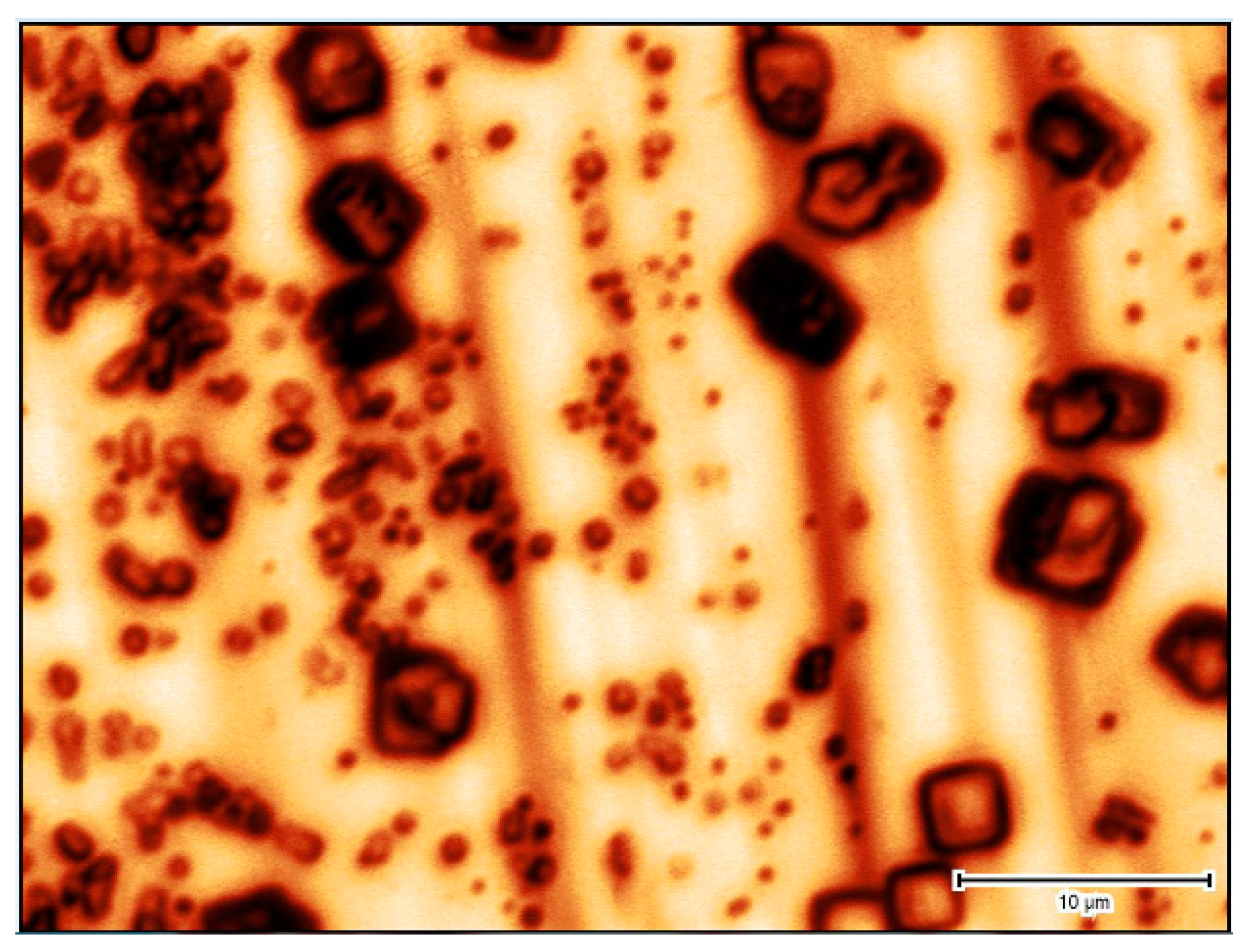
3.2.2. Gypsum Crystal Growth—Microscopic Observations

Gypsum is a monoclinic crystal and has a structure consisting of CaSO4 layers with intercalated water molecules. As a result of the weak water-layer, gypsum has a perfect 010 cleavage [120]. Over the years several studies have utilized either AFM, laser confocal microscopy, interferometry, or a combination of these methods to study the mechanisms and/or rates of gypsum crystal growth under conditions of low salinity [116,117,121,122,123,124,125,126,127,128]. For the most part, these studies have focused on the growth of the (010) surface of the crystal while in contact with stoichiometric solutions. A review of the growth mechanism on the (010) surface as depicted by these studies is given by Aquilano et al. [129] and Van Driessche et al. [66]. For the following discussion of rate equations, it should be stated that the consensus is that growth on the (010) is surface controlled and predominantly occurs by nucleation of 2D islands. Theoretically, such a growth mechanism should result in a reaction order of n = 3. Spiral dislocations that would result in a reaction order of n = 2 were observed by Van Driessche et al. [116] and Criado-Reyes et al. [128] at 80 °C. However, this was not the main step generating mechanism.
As previously mentioned, the Ca2+/SO42− ratio in solution greatly affects the thermodynamics. The only microscopic studies in which the stoichiometry of the lattice ions in solutions deviated from unity are those of Mbogoro et al. [127] and Van Driessche et al. [117]. The latter studied the growth of gypsum with natural water from the Naica mining complex in Mexico in which the Ca2+/SO42− ratio is 0.82. However, within analytical uncertainty, these waters are in equilibrium with gypsum which resulted in an ultraslow growth rate. Moreover, as gypsum ~ 1, the results of this study cannot be compared to any macroscopic rate equation for gypsum.
Mbogoro et al. [127] performed the only microscopic study that directly explored the effect of the Ca2+/SO42− ratio on the growth of gypsum. They prepared microcrystals small enough for an entire crystal to be scanned with an AFM (~10 µm) and then exposed them to oversaturated solutions (Ωgypsum 1.81–1.92) with Ca2+/SO42- molar ratios of 0.13–7.12. They observed that the face-specific rate in which different crystal faces grow responds differently to a change in the Ca2+/SO42− molar ratio. This greatly affected the habit of growing gypsum, producing plate-like crystals at low ratios and needle-like crystals at high ratios. Thus, as previously discussed, the Ca2+/SO42− ratio has a kinetic effect as well as a thermodynamic effect. This kinetic effect may affect the morphology of the crystal.
To date, the mechanisms controlling gypsum growth under saline conditions have yet to be studied at the microscopic level. While such studies are expected to shed light on gypsum growth in natural environments, handling saline and hypersaline supersaturated solutions in complex apparatuses used for direct observations is extremely challenging. Section 3.4 discusses these challenges.

3.2.3. Rate Equations of Gypsum Crystal Growth

Reaction Order for Gypsum Growth

Gypsum growth from bulk solution was studied over a wider range of environmental and chemical conditions compared with the microscopic studies [28,34,39,71,80,92,94,110,111,130,131,132,133,134,135,136,137,138]. The former conditions cover a temperature range of up to 90 °C, a pressure range of 1–100 bar, and salinities ranging from low salinity CaSO4 solutions to the hypersaline Dead Sea.
Packter [94] studied the growth of gypsum from calcium nitrate and sodium sulfate solutions and reported a reaction order of n = 4. By contrast, Barcelona and Atwood [134] studied the growth rate of gypsum precipitating from seawater and reported a reaction order of 3. As mentioned above, the latter reaction order is in accordance with the dominant growth mechanism observed on the (010) surface of gypsum. However, multiple studies have determined that the reaction order with respect to the deviation from equilibrium is n = 2 [28,39,71,92,110,111,130,131,132,134,135,136,137,138]. A reaction order of 2 does not agree with the microscopic studies of growth on the (010) surface of gypsum discussed in the previous section.
It should be noted that while the (010) surface is easily observed under the microscope, it is also the slowest growing surface of gypsum and most of the crystal volume is derived by the growth of other surfaces. This disagreement can be the result of the bias of microscopic studies towards growth on the (010) surface of gypsum, or that the reaction order that describes gypsum growth with a good empirical fit, lacks justification. This disagreement that exists between most microscopic and macroscopic studies of gypsum crystal growth requires further study.
Witkamp et al. [111] have reported that the reaction order of gypsum growth changes from 2 to 5 at high concentrations of sodium nitrate. Several other studies have observed that the reaction order depends on the distance from equilibrium: As the solution approaches equilibrium the reaction order changes to 2, whereas at the initial stage of growth, when the Ωgypsum is larger it is higher [28,92,110,132,135]. The dependency of the reaction order on Ωgypsum was suggested to be a result of different growth mechanisms dominating the close to—and far from—equilibrium growth. However, there is no direct evidence that a change in growth mechanism does indeed occur.
It has been suggested by Reznik et al. [110] that if two growth mechanisms exist, and the distance from equilibrium determines which of the two mechanisms is dominant, an additional term should be added to Equation (8) that becomes:
R a t e =   S A   [ k f a r · ( Ω 1 2 1 ) n f a r +   k c l o s e · ( Ω 1 2 1 ) n c l o s e ]
where k is a rate coefficients, and n is a reaction order with respect to the deviation from equilibrium. Subscripts far and close represent the range of deviation from equilibrium.
Based on a series of growth experiments in mixtures of Dead Sea brine with seawater (I = 4.75–9.95 m; initial Ωgypsum = 1.16–1.74; Ca2+:SO42− = 11–115) they determined that nfar = 10 and nclose = 2. Equation (9) with a reaction order of 10 and 2 for the far from—and close to—equilibrium regimes, respectively, was also found to accurately describe the growth rate of gypsum in an oversaturated (initial Ωgypsum = 2.23) reject brine collected at a desalination plant [28]. It is important to note that unlike the brines used in the experiments of Reznik et al. [110], the Ca2+/SO42− molar ratio in the reject brine collected at the desalination plant was smaller than unity (Ca2+/SO42− = 0.83) and contained a phosphonate-based antiscalant.
The effect that antiscalant has on gypsum’s precipitation kinetics in hypersaline mixtures of Dead Sea brine was recently studied by Reiss et al. [39]. Reiss et al. [39] prepared mixtures of Dead Sea brine with either rejects brine collected from a desalination plant or seawater that was evaporated until its composition, excluding the antiscalant, was similar to that of the reject brine. They conducted unseeded experiments to determine the induction times, the physical properties of the crystals that precipitate with and without the antiscalant, and the growth rate following nucleation. They also conducted seeded experiments to determine the effect of antiscalant on gypsum crystal growth when all else is equal (i.e., brine composition and crystal properties). Figure 7 presents a comparison of the measured concentration of sulfate as a function of time, to that predicted by a forward model based on Equation (9) in mixtures with a similar ratio between the Dead Sea brine and evaporated seawater or reject brine (i.e., similar composition), in seeded (Figure 7a) and unseeded (Figure 7b) experiments.
While the rate equations for both seeded experiments (Figure 7a) have a far from equilibrium (nfar = 10) and a close to equilibrium (nclose = 2) term (i.e., Equation (9)), both unseeded experiments are described by a single mechanism rate equation (i.e., Equation (8)) with a reaction order of 2. The initial Ωgypsum in all four experiments depicted in Figure 7 is the same. The difference between the seeded and unseeded experiments is the crystals. While the gypsum crystals in the seeded experiments were ground, sieved, and artificially added to the reaction cells, the crystals in the unseeded experiments nucleated from the brine within the reaction cells. Therefore, it is the properties of the solid phase and not the deviation from equilibrium that must explain the apparent “far from equilibrium” mechanism.
Cleaving or grinding a crystal may damage its surface and affect its reactivity. This may influence the rate. However, not all of the studies that observed a dependency of the reaction order on the oversaturation used ground gypsum for their experiments. Smith and Sweet [92] and Brandse et al. [132] used reagent grade CaSO4·2H2O crystals that were aged for several months in a solution as their seed material. Witkamp et al. [111] used crystals that were precipitated in the lab and left to ripen for several months. It is therefore not likely that the surfaces of the crystals in those experiments were damaged or had increased reactivity. Thus, a different explanation must be found for the observed high reaction order in those experiments. It is possible that this conundrum would only be solved by studying the growth mechanisms on additional surfaces of gypsum. To date, this issue remains unresolved.

Crystal Growth’s Rate Coefficient (k)

While the reaction order in general rate equations (Equation (8)) are said to account for the growth mechanism, the different properties of the solution and environmental conditions are represented by the rate coefficient (k). These properties include temperature, ionic strength, the stoichiometry of the lattice building ions in solution, type and concentration of the background electrolytes, and the presence of catalysts or inhibitors. Some of these properties are coupled (e.g., different ratios between the lattice ions must be accompanied by a change in the concentration of other ions, etc.) and can be difficult to isolate. Moreover, as discussed in Section 2, these properties also affect thermodynamics.
The effect temperature has on the rate coefficient can be related to the activation energy (EA) of the reaction via the Arrhenius equation. This effect was studied for the temperature range of 10–105 °C in stoichiometric solutions up to a salinity of 6 m NaCl. The rate of gypsum growth was found to increase with temperature (Figure 8) and the EA to be in the range of 60–75 kJ/mol (see table 1 in [66]).
Other properties of a solution also affect the kinetic coefficients. He et al. [71] showed that the rate coefficient in stoichiometric solutions with salinities up to 6 m NaCl increases with solubility according to:
k =   k * C S n * *
where k* and n** are proportion coefficients.
The solubility in the study of He et al. [71] was changed by salinity alone. As previously discussed, the stoichiometry of the solution also affects solubility. The solubility of gypsum in natural and industrial brines is more likely to be determined by a combination of salinity and solution stoichiometry.
Reznik et al. [110] showed that when salinity and the Ca2+/SO42− ratio are changed, the rate coefficient shows a better correlation with the equilibrium concentration of SO42− than it does with the solubility of the mineral. This may be explained by Zhang and Nancollas’s [139] suggestion that the water in the lattice of gypsum facilitate the incorporation of the more hydrated Ca2+ and that a rotational energy barrier exists for the incorporation of SO42− ions making the integration of the SO42− the rate-limiting step even when it is in excess in comparison with Ca2+. Zhang and Nancollas [139] have also suggested that Na+ competes with Ca2+ on the SO42− kink sites.
Based on the observation that the rate coefficient is correlated with SO42− concentration at equilibrium and the suggestions made by Zhang and Nancollas [139], Reznik et al. [110] have suggested the following empirical model for the rate coefficient (Equation (11) and Figure 9):
k =   r a t e i , S O 4 = 0.0065 2.0 × 10 6 × C S 0 4 4.24 1 + 2.0 × 10 6 × C S 0 4 4.24
where ratei,SO4 is the rate of SO42− integration, CSO4 is the molal concentration of sulfate in solution, 0.0065, 4.24, and 2.0 × 10⁶ are empirical coefficients that include the integration coefficient of SO42− (sec−1), the density of SO42− kink sites (mol m−2), and a coefficient related to the energy of SO42− adsorption. A detailed definition of the coefficients and their parameterization can be found in Reznik et al. [110].
Figure 9 compares the experimentally determined rate coefficients and the coefficients calculated based on Equation (11) as a function of SO42− at equilibrium and the Na+/Ca2+ activity ratio. The experimental data in Figure 9 are compiled from studies with Ca2+/SO42− molar ratio ranging from 0.1 to 43 and I up to 8.2 m. Above this ionic strength, the model did not accurately describe the rate coefficients. Reznik et al. [110] suggested that this may be due to the formation of CaSO40 complexes at high ionic strength.

3.3. Gypsum Precipitation in Large-Scale Systems

The reaction cells used during laboratory nucleation and crystal growth experiments are typically only a few hundreds of ml in volume. These reaction cells are small compared to evaporitic environments from which gypsum naturally precipitates. Following nucleation in the small reaction cells, the crystal surface-area to water ratio is very large compared to the natural situation. Moreover, in natural environments, the crystals may sink out of the water column, whereas if the water column is only a few centimeters deep, as is often the case in experiments, the crystals would remain in contact with the solution. Thus, following nucleation in the laboratory, the surface area available for crystal growth rapidly becomes large enough for crystal growth to lower the oversaturation and halt nucleation. This explains why Tind is a good proxy for the rate of nucleation. However, the relationship between nucleation and crystal growth displayed in the laboratory and natural settings often differs. This difference may result in brines that remain metastable with respect to the precipitating crystal for a long duration. In extreme cases, oversaturation may also increase as a crystal nucleates and grows.
During the winter of 1978/9, the previously stratified Dead Sea overturned [140]. Prior to the overturn, in the 1950s and 1960s, gypsum precipitated from the upper water body [141]. Shortly after the overturn it was determined that the mixed Dead Sea brine was oversaturated with respect to gypsum [142]. Since the overturn of the lake, the salinity of the Dead Sea has continued to rise and the ratio between some of the dissolved ions has shifted due to various water–rock interactions. Yet, due to sluggish kinetics of gypsum nucleation and the relatively rapid settling of the crystals out of solution, the surface area of gypsum available for growth in the lake is insufficient for growth to reduce the oversaturation [137]. As a result, today Ωgypsum of the Dead Sea brine is higher than it was 40 years ago when the lake overturned [39,142].
It should be noted that if the initial Ca2+/SO42− in solution differs from the stoichiometric ratio of the mineral, precipitation would increase the ratio between the abundant and scarce lattice ions. The Ca2+/SO42− ratio in the Dead Sea brine for example has increased from about 75 during the early 1980′s to above 130 today [39,142]. As previously discussed, a change in this ratio affects the thermodynamic settings and the kinetics of nucleation and growth.
Brines in large scale flow-through settings can remain metastable with respect to gypsum over long periods. A large pool (9.8 m3) was built near the Dead Sea to serve as a reaction chamber for large scale flow-through experiments. An oversaturated mixture of Dead Sea brine and seawater was constantly supplied to the pool over 8 months (June–January 2007). During this period, the temperature in the pool varied between 15 and 35 °C. Within a week gypsum crystals precipitated in the pool. Despite the large variation in temperature, and the presence of crystals available for growth, an Ωgypsum = 1.64 ± 0.09 was established and remained constant [143].
A steady-state oversaturation while gypsum precipitates was also found in the industrial evaporation ponds of the Atlit salt plant located on the Mediterranean coast of Israel. In this plant, a series of evaporation ponds are operated to eventually precipitate and harvest halite. In each consecutive pond, the evaporation factor is higher than in the previous one. It was observed that gypsum precipitation only began when Ωgypsum reached a value of ~1.5. After the mineral began to precipitate, Ωgypsum remained at 1.5 ± 0.2 [12].
Based on their observations, Reznik et al. [143] and Rosenberg et al. [12] suggested that under natural conditions feedback between evaporation and gypsum precipitation controls Ωgypsum of brine and the precipitation of gypsum. Evaporation increases Ωgypsum and the rate of nucleation and crystal growth. Crystal growth reduces Ωgypsum and causes faster settling of the crystals out of the water column. The settling of the crystals from the water column restricts the surface area available for growth, which enables evaporation to cause an additional increase in Ωgypsum so the rate of nucleation increases once more. Under this scenario, nucleation and crystal growth may occur simultaneously, influencing one another. This dynamic nature of gypsum precipitation is very different from the dynamics of nucleation followed by growth that is typically encountered in laboratory experiments. The different dynamics and their effect should be considered when projecting the results derived from small-scale laboratory experiments into large-scale natural environments.

3.4. Challenges of Imaging Precipitation in Brines

To date, studies at the microscale were only carried out at low salinities. Applying available microscopic techniques to study gypsum precipitation from brines may resolve some of the discrepancies between the microscopic observations at low salinities and macroscopic rate equations conducted under saline conditions. While there is a lot to learn from such studies, brines are denser than water, and can also be corrosive. Furthermore, unintended mineral phases rapidly precipitate if the liquid phase evaporates. These characters make the experimental work with brines technically challenging.
Research articles tend to focus on scientific “successes” and describe the methodologies used to produce the data. However, these methodologies are often developed by trial and error. Sharing less successful attempts and the lessons learned during the development of methods may provide meaningful and helpful insights for further research. The following discussion details challenges and difficulties that must be considered when handling brines in apparatuses used for studying water–rock interactions at the micrometer and nanometer scales. Furthermore, examples from less successful attempts are given together with outlines for solving technical issues.
The density at which gypsum precipitates from evaporating seawater is typically 10–20% higher than seawater and may reach values of up to about 1.3 g/cc [9,10,12]. Other brines that precipitate gypsum such as the Dead Sea (~1.24 g/cc) are also dense. Brine volume is not a conservative property and pump flow rates are often calibrated by volume. While these are not technical challenges, the effect of density should be considered when preparing and carrying out experiments and chemical analysis.
Halides in general and chloride in particular, are aggressive corrosion agents that harm metals and alloys [144]. Chloride is also the major anion in seawater. Subsequently, brines from marine evaporitic environments are corrosive and care should be taken to minimize contact between brines and sensitive apparatuses (e.g., Figure 10 and Figure 11).
Precipitation of other minerals as a consequence of undesired evaporation from the small experimental volume is the most challenging aspect of working with brines. This limits the use of certain techniques, and reduces the time a wet sample can be exposed to air during growth or when dried before a measurement.
Alternatives to in-situ flow-through experiments using the AFM that were previously used to study the growth of gypsum include open-air fluid cells into which an aliquot of the solution is injected by a syringe [116,127], or running ex-situ experiments in either flow-through, or batch reaction cells and drying the sample before scanning the surface [121,128,145]. If the concentration of the background electrolytes is not sufficiently low, even the slightest evaporation, under such experimental design, is sufficient to attain oversaturation and precipitation of additional mineral phases. Although Bosbach et al. [121] conducted their experiments with a low initial concentration of Ca2+ and SO42− they noted that 2D island growth sites nucleate on the surface of gypsum from the thin liquid film that remained on the surface of the mineral during the procedure of sample drying.
The problem of evaporation and precipitation of additional phases during drying is a challenge for all techniques requiring dry samples for imaging. To prevent precipitation before imaging, the solution (including any thin film) must be removed from the surface before sufficient evaporation causes oversaturation, nucleation, and growth of additional phases. Figure 12 depicts an experimental apparatus designed for in-situ water–rock interaction studies developed by Luttge and Arvidson [146].
Even with such a carefully designed experimental setup, halite precipitation was observed when attempting to study gypsum precipitation from an oversaturated (Ωgypsum = 1.75) brine (I = 3 m), which was originally undersaturated with respect to halite (Ωhalite ~ 0.1). When imaging the gypsum, halite cubes were often observed on the surface of the mineral (Figure 13).
These halite crystals occasionally appeared after short periods (several seconds) of contact with the gypsum sample. It is unlikely that during such a short time interval the solution became oversaturated with respect to halite. Rather it is more likely that halite precipitation occurred during the drying process. Indeed, optimizing the rate and angle in which the N2 jet pushes the solution towards the exit port reduced the occurrence of halite on the gypsum sample. However, a single short step of exposing the gypsum sample to the brine did not result in sufficient growth for detection. Repeated cycles of exposure increased the possibility that halite would precipitate, as the N2 jet had to be aligned perfectly over several cycles.
Overcoming precipitation of unintended minerals can also be performed by either increasing the degree of oversaturation and precipitation potential of the desired phase or lowering the salinity of the brine. Lowering the salinity may extend the duration in which the thin film can be removed from the gypsum sample before halite becomes oversaturated and precipitates.
The technical difficulties and challenges arising from the properties of brines that are presented here should not be a barrier for studying gypsum precipitation under saline conditions at the scale at which crystal–brine interactions occur. However, these challenges should be considered and merit careful attention when designing the protocol and carrying out such a study.

4. Crystal Habit and Size Distribution

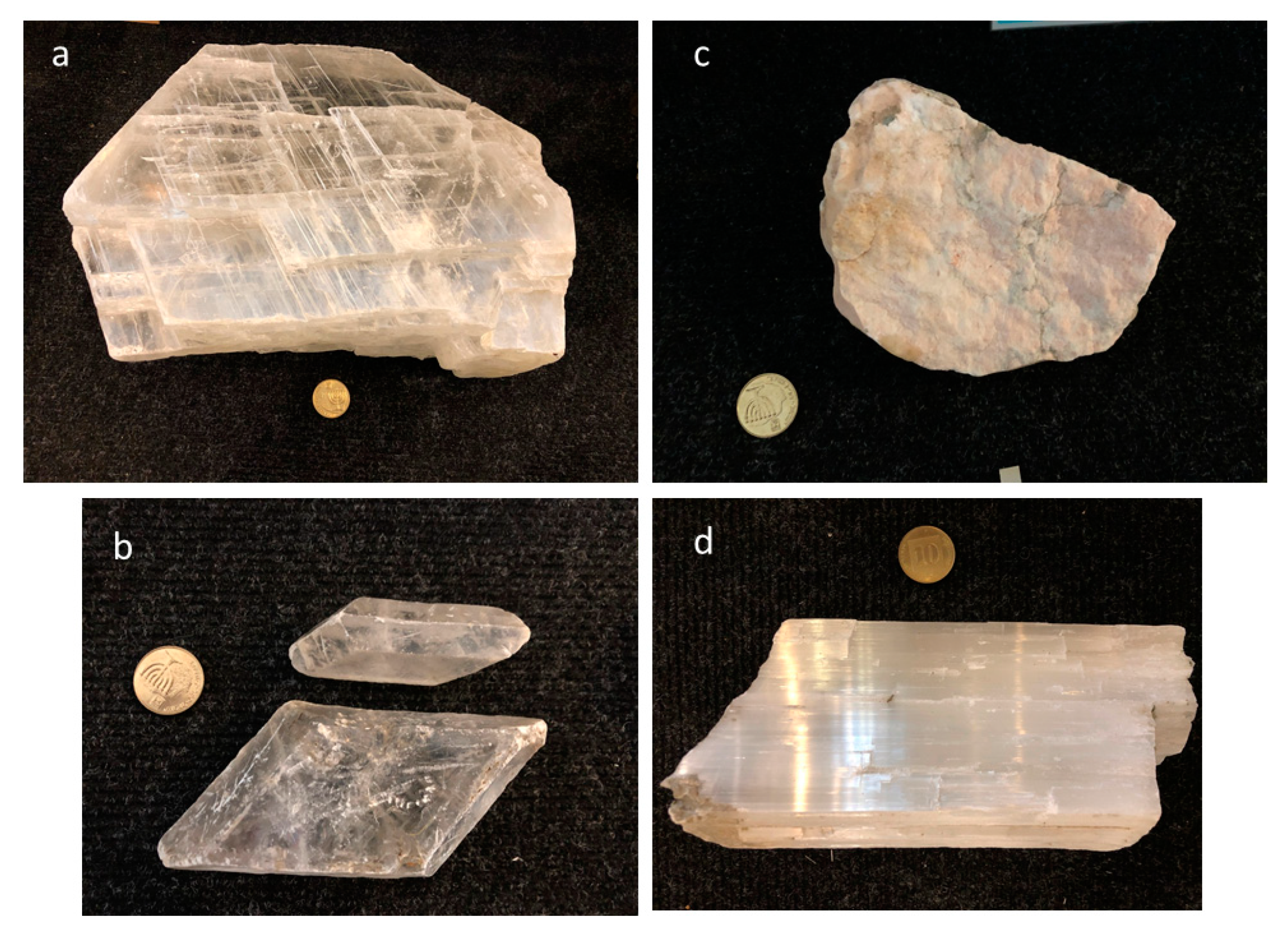
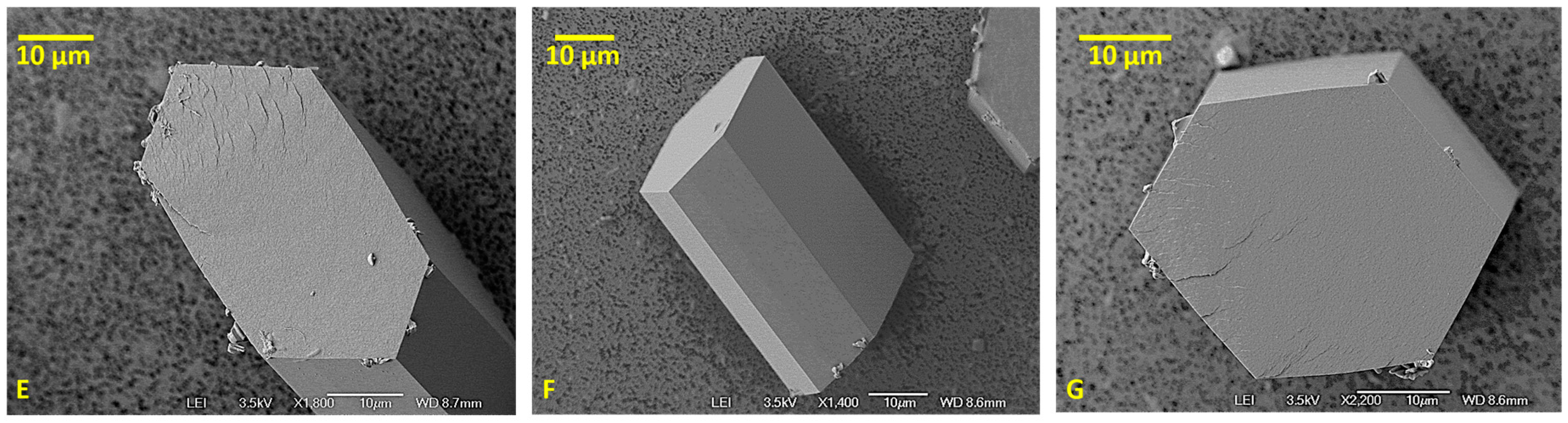
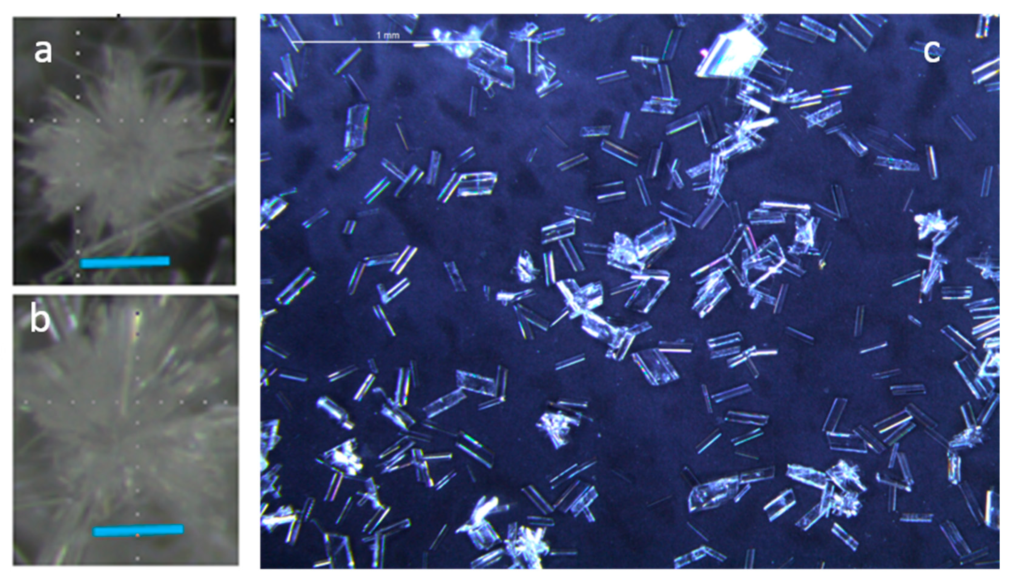
4.1. Gypsum Morphology

Gypsum appears in various forms. In nature gypsum pre-dominantly appears as selenite, alabaster, or satin spar (Figure 14). Alabaster and satin spar are aggregates. Whereas the orientation of the crystals forming alabaster is randomly distributed, the crystals in satin spar are attached along their length axis. Selenite is mostly found as idiomorphic single crystals that are often twinned [148] and may form mega-crystals. Famous amongst these are the Naica mine selenite with dimensions that exceed 10 × 1 m and are the largest naturally occurring crystals known to humans [149].
Gypsum is a monoclinic crystal often defined by the c2/c space group. With this convention, the main crystal surfaces are the (010), (120), (111), and (011). However, the unit cell of the mineral can be reasonably represented by different selections. As different selections can be made, the same gypsum face can be found in the literature with different Miller indexes. This multiple assignments of indexes is a cause for confusion. Indeed, different selections were made to represent a crystal and growth elements on that same crystal [150]. An overview of the different reasonable selections and the transformation matrices between the different unit cells is discussed in a previous review by Aquilano et al. [129].
The bonding energy of lattice ions to the different surfaces of a single crystal vary. If one assumes that the morphology of a crystal would correlate to the minimum energy (i.e., “equilibrium morphology”), then thermodynamic considerations of energy minimization can be used to explain and predict the morphology of a crystal. Previous studies have studied the equilibrium morphology of gypsum ([129,151,152,153], and references within) with varying degrees of agreement between theoretical calculations and observed crystal morphology. However, other studies have shown that the morphology of gypsum is affected by the presence of organic [134,154,155,156] or inorganic [88,156,157,158] ions or molecules including commercially used scale inhibitors [39,131,145,159,160].
The “growth morphology” of a crystal is shaped by the relative growth rate of the different crystal faces. As such, it is affected by factors that influence growth kinetics such as the ratio between the lattice ions in solution, the presence of organic and inorganic molecules, or ions, etc. Thus, the morphology of gypsum in natural and industrial brines cannot be explained solely by thermodynamic considerations.
Reiss et al. [158] have recently studied the morphology of gypsum single-crystals precipitating from oversaturated hypersaline mixtures of calcium-rich Dead Sea brine (Ca2+/SO42− ~ 130) and sulfate-rich seawater (Ca2+/SO42− ~ 0.36). The different mixtures were each enriched with calcium and sulfate salts in order to control and increase the oversaturation without altering the Ca2+/SO42− ratio of the solution. Different hypersaline compositions with a similar Ca2+/SO42− ratio (~13, 24, and 45) were prepared with Ωgypsum of ~ 1.7–7. The ionic strength of the experiments ranged from 5.5 to 10 m. Each mixture was divided into aliquots. At designated times, the crystals from a given aliquot were separated from the solution and studied. The study showed that individual crystals that have precipitated from a given aliquot had different morphologies (Figure 15), implying that the effect of brine composition on crystal habit must be viewed in terms of crystal populations. Reiss et al. [158] therefore suggested to use the average aspect ratio (crystal length/crystal width) of crystal populations that precipitated from different aliquots to distinguish between the habits of populations that precipitated from different compositions. This statistical approach, which highlights the differences between crystal populations while averaging out the different morphologies of individual crystals comprising a population, was found to be useful in studying the effect brine composition has on gypsum crystal habit.
The Ca2+/SO42− molar ratio in Dead Sea–seawater mixtures decreases with the % wt. seawater. The study found that at a given Ωgypsum, the crystal population’s average aspect ratio increases (i.e., the gypsum crystals have become more elongated) with an increase in % wt. seawater in such mixture [158]. This is contrary to the results of experiments conducted with simple low ionic strength solutions that found that the aspect ratio of single crystals of gypsum increases with an increase in Ca2+/SO42− ratio ([127], and references within). In the case of Reiss et al. [158], changing the ratio between the two end-members also changes the concentration of the various background electrolytes. The presence of major cations in solutions, particularly Mg2+, has already been reported to increase the aspect ratio of gypsum [88]. Since Mg2+ is the major cation in the Dead Sea, its presence should also cause elongation of the gypsum as the fraction of the Dead Sea in solution increases. The contradictions between the effect the Ca2+/SO42− ratio and Mg2+ have on the habit of gypsum precipitating under low ionic strengths and hypersaline Dead Sea–seawater mixtures is yet to be explained.
A microscopic study that focuses on the kinetics of growth of individual surfaces and the mechanisms that drive the growth may be required to resolve this conundrum. However, conducting such experiments is a challenging task (Section 3.4).
At above Ωgypsum = 3 the habit of the gypsum precipitated from Dead Sea–seawater mixtures changed from idiomorphic (needle-like or tabular) to stellate (also termed rosette or spherulite morphology) (Figure 16). Such a change in morphology with an increase in oversaturation is not unique for gypsum and is known to occur in many natural and industrial solids (i.e., crystals, polymers, metallic glasses., etc.) [161] and has also already been reported for gypsum [29,162].
A plot of the logarithm of the measured Tind versus 1/log2(Ω) for solutions with a similar composition but different Ω gives two linear lines with different slopes and intercepts (Figure 17). The oversaturation at which these lines intersect is interpreted, based on the CNT (Equation (3)), as the oversaturation at which the dominant nucleation mechanism changes from homogenous to heterogeneous [78]. For gypsum, this change of slope reportedly occurs between 2.15 and 4.4 [77,79,99,100,162]. Reznik et al. [79] have determined that for Dead Sea–seawater mixtures the slope changes over Ωgypsum range of 2.8–3.7 (Figure 17). Thus, the idiomorphic crystals observed by Reiss et al. [158] at Ωgypsum ≤ 3 correspond to the heterogeneous nucleation range while the stellate crystals at Ωgypsum ≥ 4 correspond to the homogenous nucleation range. This is also in agreement with the study of Alimi and Gadri [162] who observed idiomorphic and stellate crystals at Ωgypsum that correspond, respectively, to the heterogeneous and homogenous regions in their experiments. Alimi and Gadri [162] have attributed the change in gypsum morphology to the change in the mechanism of nucleation.
While Tind is considered a proxy for the rate of nucleation, it also includes the initial stages of crystal growth [78]. Single crystals with an equal mass would have a larger surface area if their morphology is stellate rather than idiomorphic. Thus, all else being equal, a change in the habit of gypsum from idiomorphic needle-like or tabular to stellate would lower the induction times in proportion with the increased surface area. This will affect the slope of a log(Tind) versus 1/log2(Ω) plot. It is, therefore, possible that the change of slopes, is a result of a morphological change rather than an actual change in the dominant mechanism of nucleation.
Alternative explanations to the formation of stellate morphology, other than heterogeneous vs. homogeneous nucleation are: a) surface nucleation that can affect the diffusion field around the crystal or create a polycrystalline “mineral”, or b) agglomeration/attachment of particles [163] Recently Stawski et al. [164] studied the internal structure of gypsum. Their study suggests that single crystals of gypsum are mesocrystals, i.e., crystals that are built of distinguishable sub-domains but have defined crystal surfaces and diffract as a single crystal. Based on this observation they suggested that the stellate morphology is an external representation of internal misalignment of the internal sub-domains. Such misalignment develops when the sub-domain aggregation becomes rapid compared to the diffusion of the water molecules within the forming lattice. This supports the formation of stellate gypsum at elevated oversaturation by a process of agglomeration, rather than a transformation between heterogeneous and homogenous nucleation.
Previous publications, including by some of the co-authors of this paper, have suggested that understanding the effects that brine composition has on the morphology and habit of gypsum can help in determining the paleo-conditions from which gypsum has precipitated [128,156,165]. Yet, the study by Reiss et al. [158] is, to our knowledge, the only study to explicitly explore the effect of brine composition on the morphology of gypsum under hypersaline conditions with multiple background electrolytes. The discrepancies between the suggested effects of Ca2+/SO42− and Mg2+ on gypsum habit between the latter study and previous studies performed at low salinities are unexplained. Thus, further research is required before the morphology of gypsum could be used to determine the conditions from which gypsum precipitates in saline environments.

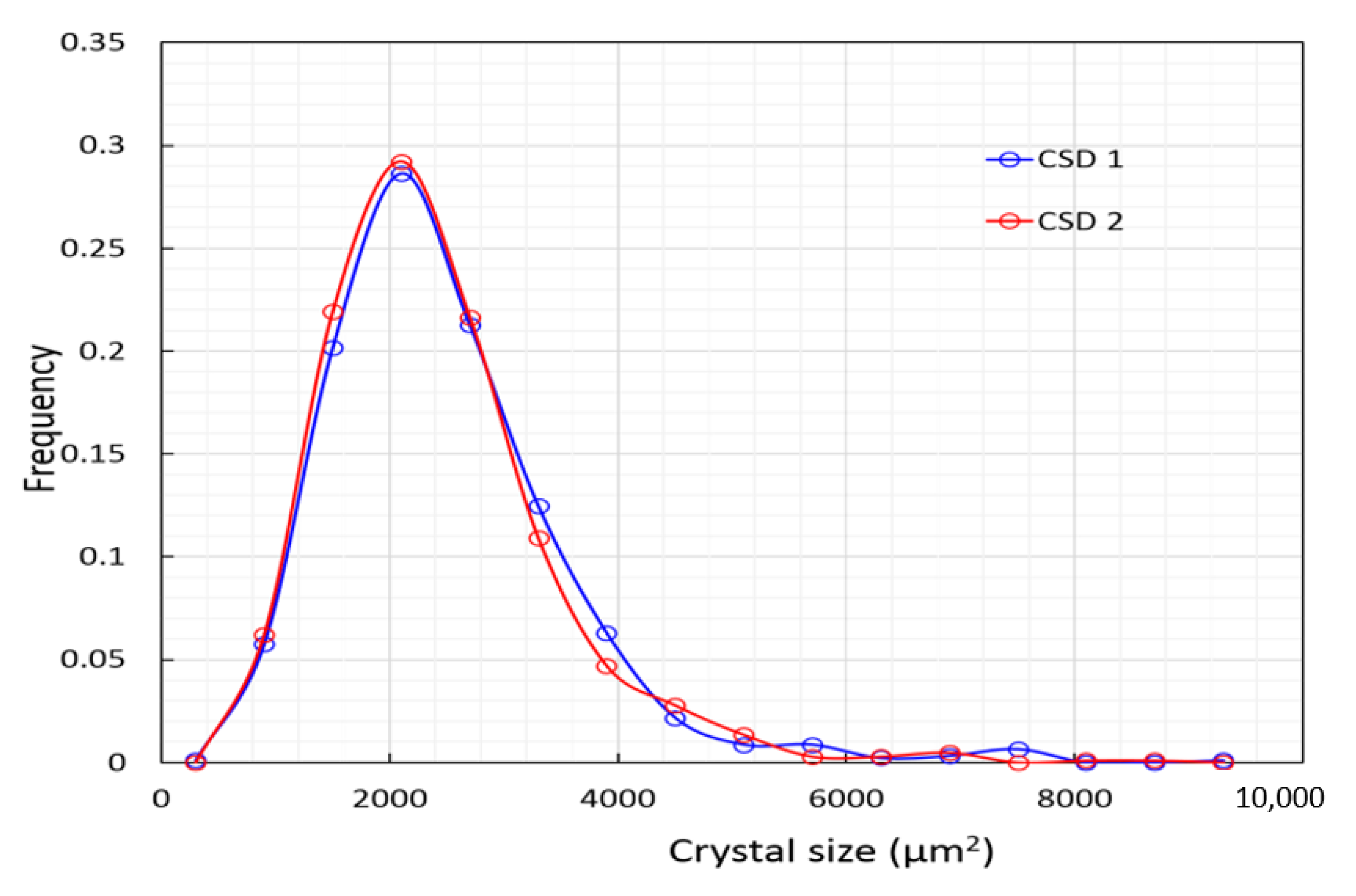
4.2. Gypsum—Crystal Size Distribution and Its Implications

The crystal size distribution (CSD) of a given crystal population embodies the chemical (i.e., nucleation, growth, and dissolution) and physical (i.e., agglomeration or breakage of crystals) processes that have affected the individual crystals. If the mutual effect of these processes is understood, then the CSD can be used to interpret the geological history under which the crystal population has developed. In fact, the CSD of gypsum was recently used to interpret the paleo-conditions on Mars [22]. Gypsum is also manufactured for different purposes and forms undesired scale. Therefore, the CSD of gypsum is important in various industrial processes. For example, the CSD of gypsum determines the filtration rate during wet industrial processes in which the mineral precipitates [166]. Thus, understanding the interaction between the chemical and physical processes, and the mechanisms that control gypsum shape and size, may help develop protocols to direct the precipitation process towards the formation of preferable CSDs.
CSD of gypsum is also a crucial parameter that would determine some of the environmental impacts on the Dead Sea if and when seawater or reject brine from desalination will be introduced to the Dead Sea. As shown above, mixing between these two waters will lead to gypsum precipitation. The CSD of this gypsum will determine if the crystals will quickly settle to the bottom or remain suspended and whiten the surface waters [167].
Lognormal size distribution is a distribution in which the logarithm of the size is normally distributed. Different studies have shown that the CSD of gypsum populations precipitated in natural environments [168], on desalination membranes [29], and from batch solutions of hypersaline brines [158] follow a lognormal distribution (Figure 18). Kah et al. [22] have recently studied the size distribution of pseudo-morphs after gypsum in Gale Crater, Mars. The size of these pseudo-morphs which have retained the characteristics of the original mineral assemblage, also follows a lognormal distribution.
The mathematical generation of a lognormal distribution has been discussed within the theoretical realm of statistics and within the context of geological or biological processes [169,170,171,172]. However, currently, no liable physical model to generate a lognormal CSD is compatible with crystal growth in which at a certain Δtime, a given surface of a given crystal (e.g., 010, 120, etc. for gypsum) would grow by a constant Δlength regardless of crystal size. Thus, growth models that relate growth rate to the deviation from equilibrium cannot explain the size distribution of gypsum.
The realization that geologic samples, including grain size in sediments and minerals in rocks, often follow or closely approximate a lognormal distribution has been made decades ago. Middleton [169] had made the first rigorous attempt to explain the development of such CSD within a geological context. He showed that a lognormal distribution can be mathematically modelled in several ways, and mathematically describe the lognormal distribution in sediments. However, Middleton [169] also noted that his model pre-supposed probability assumptions that are not necessarily valid from the underlying physical process. He then concluded that to be convincing, the proposed model should: a) be based on principal assumptions of physical nature, and b) be able to explain deviations from a lognormal distribution.
Eberl and co-authors [168,170,173,174,175] have studied CSD in geologic materials and developed a mathematical framework for interpreting the geologic history based on the CSD. According to their mathematical framework, the initial CSD is determined by the conditions under which nucleation occurs (constant nucleation, decreasing nucleation rate, etc.) and subsequent crystal growth that follows the law of proportionate effect (LPE) shapes the distribution. According to LPE, crystal growth is described by [169,170]:
X j + 1 =   X j +   ε j X j
where X is crystal size and ε is a random positive value that in each growth cycle varies between 0 and 1. Subscripts j and j + 1 represent the growth cycle.
Growth according to LPE has been able to accurately describe the lognormal distribution of many naturally formed crystal populations, as well as deviations from such a distribution [168,170,173,174,175]. However, contrary to the deterministic nature of rate equations, the LPE as presented in Equation (12) is probabilistic. Moreover, according to Equation (12), the growth of a crystal depends on its previous size (i.e., Xj) and it has a random element to it (i.e., εj). Thus, according to LPE, crystals having the same size may grow at different rates and larger crystals are likely to grow faster than small crystals. Such behavior is in stark contrast to crystal growth theory that relates growth rate to the deviation from equilibrium.
At the nanometer and micrometer scales, the interfacial tension depends on crystal size. Adding a term relating the interfacial tension to crystal size into standard rate equations demonstrates that the growth of small crystals is size-dependent [176]. However, Eberl et al. [168] have not limited the size-dependent growth to any particular scale and have used the LPE theory to describe CSD of gypsum with crystals ranging from about 0.5–15 cm.
The ability of LPE growth to describe a lognormal distribution and the typical deviations from this distribution satisfy Middleton’s second requirement [169]. However, Eberl et al. [168] have conceded that “there are no obvious thermodynamic or kinetic reasons to assume that ions would be transported or incorporated into a crystal at a rate that is proportionate to its diameter” and that the exact mechanism leading to proportionate growth is not adequately explained in the literature. They have later suggested that size-dependent growth may be due to fluid dynamics being turbulent around larger crystals. However, the results of their experiments to test this hypothesis were inconclusive [166]. Thus, to date, LPE growth cannot be explained by physical principals and this growth model does not fulfill Middleton’s requirement that a model would be based on the assumption of physical nature.
Currently, CSDs cannot be explained by typical precipitation paradigms, while explanations of the evolution of CSD for geological materials do not comply with the accepted paradigms of growth. It should be stated that while LPE growth is compatible with the development of lognormal CSD and accurately replicates both this CSD and deviations from it, the theory only considers chemical processes. Reiss et al. [158] have recently suggested that agglomeration of particles during the early stages of gypsum precipitation may be a mechanism affecting the final CSD. This suggestion is in agreement with the observation made by Stawski et al. [164] that gypsum crystals are mesocrystals. However, the extent to which agglomeration shapes the final CSD still requires further study.

5. Summary and Outline for Future Research

The abundance of gypsum in the geological record and its precipitation under various conditions in both natural and engineered environments make this mineral and its precipitation significant in many fields of science and engineering. Therefore, the study of gypsum and its precipitation has been the focus of many studies over the last decades. In this article, we outlined the current knowledge regarding the thermodynamics involved in the precipitation of gypsum, the kinetics of nucleation and growth, and the effect of the above on the morphology and size distribution of the precipitating gypsum.
Discrepancies exist between experimental studies of gypsum precipitation from low salinity and high salinity solutions. Moreover, disagreement exists between microscopic and macroscopic observations. These discrepancies include the reaction order of gypsum and the mechanisms that control it, the effect of brine composition and the Ca2+/SO42− ratio in solution on the habit of gypsum, the mechanism by which Mg2+ retards the nucleation and growth of gypsum. Moreover, the nucleation pathway and growth mechanisms of gypsum under saline conditions have yet to be studied with the advanced techniques available today to observe and image reactions at the micrometer and nanometer scales at which crystal–water interactions occur. While such studies will greatly increase our understanding of these reactions in the natural and industrial conditions at which they occur, such experiments are challenging. Moreover, the lognormal CSD of gypsum (and other minerals) remains an enigma that requires further consideration by the community. Thus, while the last decades have resulted in a tremendous advance in our understanding of gypsum and its precipitation, many questions remain to be answered.

Author Contributions

Data curation, A.G.R.; writing—original draft preparation, A.G.R.; writing—review and editing, I.G., Y.O.R., I.J.R., A.L., S.E. and J.G. All authors have read and agreed to the published version of the manuscript.

Funding

Not applicable.

Institutional Review Board Statement

Not applicable.

Informed Consent Statement

Not applicable.

Data Availability Statement

Not applicable.

Acknowledgments

We wish to thank the editors of this special issue, A.E.S Van Driessche and T.M. Stawski for inviting us to write this paper. We also wish to thank the three reviewers who have kindly taken the time to read and comment on this manuscript.

Conflicts of Interest

The authors declare no conflict of interest.

References

  1. Nabhan, S.; Luber, T.; Scheffler, F.; Heubeck, C. Climatic and geochemical implications of Archean pedogenic gypsum in the Moodies Group (~3.2Ga), Barberton Greenstone Belt, South Africa. Precambrian Res. 2016, 275, 119–134. [Google Scholar] [CrossRef]
  2. Lugli, S.; Manzi, V.; Roveri, M.; Schreiber, B.C. The Primary Lower Gypsum in the Mediterranean: A new facies interpretation for the first stage of the Messinian salinity crisis. Palaeogeogr. Palaeoclimatol. Palaeoecol. 2010, 297, 83–99. [Google Scholar] [CrossRef]
  3. Thompson, J.B.; Ferris, F.G. Cyanobacterial precipitation of gypsum, calcite, and magnesite from natural alkaline lake water. Geology 1990, 18, 995–998. [Google Scholar] [CrossRef]
  4. Levy, E.J.; Sivan, O.; Antler, G.; Lazar, B.; Stein, M.; Yechieli, Y.; Gavrieli, I. Mount Sedom salt diapir - Source for sulfate replenishment and gypsum supersaturation in the last glacial Dead Sea (Lake Lisan). Quat. Sci. Rev. 2019, 221, 105871. [Google Scholar] [CrossRef]
  5. White, S.N.; Dunk, R.M.; Peltzer, E.T.; Freeman, J.J.; Brewer, P.G. In situ Raman analyses of deep-sea hydrothermal and cold seep systems (Gorda Ridge and Hydrate Ridge). Geochemistry, Geophys. Geosystems 2006, 7. [Google Scholar] [CrossRef]
  6. Tang, M.; Ehreiser, A.; Li, Y.-L. Gypsum in modern Kamchatka volcanic hot springs and the Lower Cambrian black shale: Applied to the microbial-mediated precipitation of sulfates on Mars. Am. Mineral. 2014, 99, 2126–2137. [Google Scholar] [CrossRef] [Green Version]
  7. Alt, J.C.; Davidson, G.J.; Teagle, D.A.H.; Karson, J.A. Isotopic composition of gypsum in the Macquarie Island ophiolite: Implications for the sulfur cycle and the subsurface biosphere in oceanic crust. Geology 2003, 31, 549–552. [Google Scholar] [CrossRef]
  8. Ochsenius, C. On the Formation of Rock-Salt Beds and Mother-Liquor Salts. Proc. Acad. Nat. Sci. Philadelphia 1888, 40, 181–187. [Google Scholar]
  9. Raup, O.B. Gypsum Precipitation By Mixing Seawater Brines. Am. Assoc. Pet. Geol. Bull. 1982, 66, 363–367. [Google Scholar] [CrossRef]
  10. McCaffrey, M.A.; Lazar, B.; Holland, H.D. The evaporation path of seawater and the coprecipitation of Br and K+ with halite. J. Sediment. Petrol. 1987, 57, 928–937. [Google Scholar] [CrossRef]
  11. Lazar, B.; Starinsky, A.; Katz, A.; Sass, E.; Ben-Yaakov, S. The carbonate system in hypersaline solutions: Alkalinity and CaCO3 solubility of evaporated seawater. Limnol. Oceanogr. 1983, 28, 978–986. [Google Scholar] [CrossRef]
  12. Rosenberg, Y.O.; Sade, Z.; Ganor, J. The precipitation of gypsum, celestine, and barite and coprecipitation of radium during seawater evaporation. Geochim. Cosmochim. Acta 2018, 233, 50–65. [Google Scholar] [CrossRef]
  13. Braitsch, O. Salt Deposits Their Origin and Composition; Springer Science & Business Media: Salt Lake City, UT, USA, 1971. [Google Scholar]
  14. Stein, M. The sedimentary and geochemical record of neogene-quaternary water bodies in the Dead Sea basin - Inferences for the regional paleoclimatic history. J. Paleolimnol. 2001, 26, 271–282. [Google Scholar] [CrossRef]
  15. Stein, M.; Starinsky, A.; Katz, A.; Goldstein, S.L.; Machlus, M.; Schramm, A. Strontium isotopic, chemical, and sedimentological evidence for the evolution of Lake Lisan and the Dead Sea. Geochim. Cosmochim. Acta 1997, 61, 3975–3992. [Google Scholar] [CrossRef]
  16. Szynkiewicz, A.; Ewing, R.C.; Moore, C.H.; Glamoclija, M.; Bustos, D.; Pratt, L.M. Origin of terrestrial gypsum dunes-Implications for Martian gypsum-rich dunes of Olympia Undae. Geomorphology 2010, 121, 69–83. [Google Scholar] [CrossRef]
  17. Ryan, W.B.F. Decoding the mediterranean salinity crisis. Sedimentology 2009, 56, 95–136. [Google Scholar] [CrossRef]
  18. Eardley, A. Gypsum dunes and evaporite history of the Great Salt Lake Desert. Utah Geological and Mineralogical Survey 1962.
  19. Langevin, Y.; Poulet, F.; Bibring, J.P.; Gondet, B. Sulfates in the north polar region of Mars detected by OMEGA/Mars express. Science 2005, 307, 1584–1586. [Google Scholar] [CrossRef]
  20. Gendrin, A.; Mangold, N.; Bibring, J.P.; Langevin, Y.; Gondet, B.; Poulet, F.; Bonello, G.; Quantin, C.; Mustard, J.; Arvidson, R.; et al. Sulfates in Martian layered terrains: The OMEGA/Mars express view. Science 2005, 307, 1587–1591. [Google Scholar] [CrossRef] [Green Version]
  21. Squyres, S.W.; Grotzinger, J.P.; Arvidson, R.E.; Bell, J.F.; Calvin, W.; Christensen, P.R.; Clark, B.C.; Crisp, J.A.; Farrand, W.H.; Herkenhoff, K.E.; et al. In situ evidence for an ancient aqueous environment at Meridiani Planum, Mars. Science 2004, 306, 1709–1714. [Google Scholar] [CrossRef] [Green Version]
  22. Kah, L.C.; Stack, K.M.; Eigenbrode, J.L.; Yingst, R.A.; Edgett, K.S. Syndepositional precipitation of calcium sulfate in Gale Crater, Mars. Terra Nova 2018, 30, 431–439. [Google Scholar] [CrossRef]
  23. Farías, M.E.; Contreras, M.; Rasuk, M.C.; Kurth, D.; Flores, M.R.; Poiré, D.G.; Novoa, F.; Visscher, P.T. Characterization of bacterial diversity associated with microbial mats, gypsum evaporites and carbonate microbialites in thalassic wetlands: Tebenquiche and La Brava, Salar de Atacama, Chile. Extremophiles 2014, 18, 311–329. [Google Scholar] [CrossRef] [PubMed]
  24. Warren, J.K. The hydrological setting, occurrence and significance of gypsum in late Quaternary salt lakes in South Australia. Sedimentology 1982, 29, 609–637. [Google Scholar] [CrossRef]
  25. Sinha, R.; Raymahashay, B.C. Evaporite mineralogy and geochemical evolution of the Sambhar Salt Lake, Rajasthan, India. Sediment. Geol. 2004, 166, 59–71. [Google Scholar] [CrossRef]
  26. Hacini, M.; Kherici, N.; Oelkers, E.H. Mineral precipitation rates during the complete evaporation of the Merouane Chott ephemeral lake. Geochim. Cosmochim. Acta 2008, 72, 1583–1597. [Google Scholar] [CrossRef]
  27. Gibson, G.W. Geological Investigations in Southern Victoria Land, Antarctica. New Zeal. J. Geol. Geophys. 1962, 5, 361–374. [Google Scholar] [CrossRef]
  28. Rosenberg, Y.O.; Reznik, I.J.; Zmora-Nahum, S.; Ganor, J. The effect of pH on the formation of a gypsum scale in the presence of a phosphonate antiscalant. Desalination 2012, 284, 207–220. [Google Scholar] [CrossRef]
  29. Karabelas, A.J.; Karanasiou, A.; Mitrouli, S.T. Incipient membrane scaling by calcium sulfate during desalination in narrow spacer-filled channels. Desalination 2014, 345, 146–157. [Google Scholar] [CrossRef]
  30. Uchymiak, M.; Lyster, E.; Glater, J.; Cohen, Y. Kinetics of gypsum crystal growth on a reverse osmosis membrane. J. Memb. Sci. 2008, 314, 163–172. [Google Scholar] [CrossRef]
  31. Rosenbauer, R.J.; Bischoff, J.L.; Kharaka, Y.K. Geochemical effects of deep-well injection of the Paradox Valley brine into Paleozoic carbonate rocks, Colorado, U.S.A. Appl. Geochemistry 1992, 7, 273–286. [Google Scholar] [CrossRef]
  32. Regenspurg, S.; Feldbusch, E.; Byrne, J.; Deon, F.; Driba, D.L.; Henninges, J.; Kappler, A.; Naumann, R.; Reinsch, T.; Schubert, C. Mineral precipitation during production of geothermal fluid from a Permian Rotliegend reservoir. Geothermics 2015, 54, 122–135. [Google Scholar] [CrossRef]
  33. Rendel, P.M.; Gavrieli, I.; Wolff-Boenisch, D.; Ganor, J. Gypsum solubility under pressure conditions relevant to CO2 geological storage. Int. J. Greenh. Gas Control 2016, 55, 15–22. [Google Scholar] [CrossRef]
  34. Rendel, P.M.; Gavrieli, I.; Ben-Eliahu, N.; Wolff-Boenisch, D.; Ganor, J. Gypsum crystal growth kinetics under conditions relevant to CO2 geological storage. Int. J. Greenh. Gas Control 2019, 91, 102829. [Google Scholar] [CrossRef]
  35. Dávila, G.; Luquot, L.; Soler, J.M.; Cama, J. Interaction between a fractured marl caprock and CO2-rich sulfate solution under supercritical CO2 conditions. Int. J. Greenh. Gas Control 2016, 48, 105–119. [Google Scholar] [CrossRef] [Green Version]
  36. Lattemann, S.; Höpner, T. Environmental impact and impact assessment of seawater desalination. Desalination 2008, 220, 1–15. [Google Scholar] [CrossRef]
  37. Mady, M.F.; Charoensumran, P.; Ajiro, H.; Kelland, M.A. Synthesis and Characterization of Modified Aliphatic Polycarbonates as Environmentally Friendly Oilfield Scale Inhibitors. Energy and Fuels 2018, 32, 6746–6755. [Google Scholar] [CrossRef]
  38. Hasson, D.; Shemer, H.; Sher, A. State of the art of friendly “green” scale control inhibitors: A review article. Ind. Eng. Chem. Res. 2011, 50, 7601–7607. [Google Scholar] [CrossRef]
  39. Reiss, A.G.; Gavrieli, I.; Ganor, J. The effect of phosphonate-based antiscalant on gypsum precipitation kinetics and habit in hyper-saline solutions: An experimental and modeling approach to the planned Red Sea – Dead Sea Project. Desalination 2020, 496, 114638. [Google Scholar] [CrossRef]
  40. Van Santen, R.A. The Ostwald step rule. J. Phys. Chem. 1984, 88, 5768–5769. [Google Scholar] [CrossRef]
  41. Pitzer, K.S. Thermodynamics of electrolytes. I. Theoretical basis and general equations. J. Phys. Chem. 1973, 77, 268–277. [Google Scholar] [CrossRef] [Green Version]
  42. Pitzer, K.S.; Mayorga, G. Thermodynamics of electrolytes. II. Activity and osmotic coefficients for strong electrolytes with one or both ions univalent. J. Phys. Chem. 1973, 77, 2300–2308. [Google Scholar] [CrossRef] [Green Version]
  43. Pitzer, K.S.; Mayorga, G. Thermodynamics of electrolytes. III. Activity and osmotic coefficients for 2-2 electrolytes. J. Solution Chem. 1974, 3, 539–546. [Google Scholar] [CrossRef] [Green Version]
  44. Pitzer, K.S. Thermodynamics of electrolytes. V. effects of higher-order electrostatic terms. J. Solution Chem. 1975, 4, 249–265. [Google Scholar] [CrossRef] [Green Version]
  45. Pitzer, K.S.; Kim, J.J. Thermodynamics of Electrolytes. IV. Activity and Osmotic Coefficients for Mixed Electrolytes. J. Am. Chem. Soc. 1974, 96, 5701–5707. [Google Scholar] [CrossRef] [Green Version]
  46. Harvie, C.E.; Weare, J.H. The prediction of mineral solubilities in natural waters: The NaKMgCaClSO4H2O system from zero to high concentration at 25° C. Geochim. Cosmochim. Acta 1980, 44, 981–997. [Google Scholar] [CrossRef]
  47. Moeller, N. The prediction of mineral solubilities in natural waters: A chemical equilibrium model for the Na-Ca-Cl-SO_4-H_2O system, to high temperature and concentration. Geochim. Cosmochim. Acta 1988, 52, 821–837. [Google Scholar] [CrossRef]
  48. Krumgalz, B.S.; Millero, F.J. Physico-chemical study of dead sea waters. III. On gypsum saturation in Dead Sea waters and their mixtures with Mediterranean Sea water. Mar. Chem. 1983, 13, 127–139. [Google Scholar] [CrossRef]
  49. Krumgalz, B.S.; Millero, F.J. Physico-chemical study of the dead sea waters. I. Activity coefficients of major ions in dead sea water. Mar. Chem. 1982, 11, 209–222. [Google Scholar] [CrossRef]
  50. Krumgalz, B.S. Application of the pitzer ion interaction model to natural hypersaline brines. J. Mol. Liq. 2001, 91, 3–19. [Google Scholar] [CrossRef]
  51. Harvie, C.E.; Møller, N.; Weare, J.H. The prediction of mineral solubilities in natural waters: The Na-K-Mg-Ca-H-Cl-SO4-OH-HCO3-CO3-CO2-H2O system to high ionic strengths at 25°C. Geochim. Cosmochim. Acta 1984, 48, 723–751. [Google Scholar] [CrossRef]
  52. Toner, J.D.; Catling, D.C.; Light, B. A revised Pitzer model for low-temperature soluble salt assemblages at the Phoenix site, Mars. Geochim. Cosmochim. Acta 2015, 166, 327–343. [Google Scholar] [CrossRef]
  53. Appelo, C.A.J. Principles, caveats and improvements in databases for calculating hydrogeochemical reactions in saline waters from 0 to 200°C and 1 to 1000atm. Appl. Geochem. 2015, 55, 62–71. [Google Scholar] [CrossRef]
  54. Oelkers, E.H.; Bénézeth, P.; Pokrovski, G.S. Thermodynamic databases for water-rock interaction. Rev. Mineral. Geochem. 2009, 70, 1–46. [Google Scholar] [CrossRef]
  55. Parkhurst, D.L.; Appelo, C.A.J. User’s Guide to PHREEQC (Version 2): A Computer Program for Speciation, Batch-Reaction, One-Dimensional Transport, and Inverse Geochemical Calculations. In Water-resources investigations report 99.4259; USGS: Reston, VA, USA, 1999. [Google Scholar]
  56. Parkhurst, D.L.; Appelo, C.A.J. Description of Input and Examples for PHREEQC Version 3—A Computer Program for Speciation, Batch-Reaction, One-Dimensional Transport, and Inverse Geochemical Calculations. In U.S. Geological Survey Techniques and Methods; book 6, chapter A43; USGS: Reston, VA, USA, 2013; ISBN 0092-332X. [Google Scholar]
  57. Plummer, L.N.; Parkhurst, D.L.; Fleming, G.W.; Dunkle, S. A Computer Program Incorporating Pitzer’s Equations for Calculation of Geochemical Reactions in Brines; U.S. Geological Survey: Washington, DC, USA, 1988. [Google Scholar]
  58. Reznik, I.J.; Ganor, J.; Gal, A.; Gavrieli, I. Gypsum saturation degrees and precipitation potentials from Dead Seaseawater mixtures. Environ. Chem. 2009, 6, 416–423. [Google Scholar] [CrossRef]
  59. Appelo, C.A.J.; Parkhurst, D.L.; Post, V.E.A. Equations for calculating hydrogeochemical reactions of minerals and gases such as CO 2 at high pressures and temperatures. Geochim. Cosmochim. Acta 2014, 125, 49–67. [Google Scholar] [CrossRef]
  60. Rendel, P.M.; Wolff-Boenisch, D.; Gavrieli, I.; Ganor, J. A novel experimental system for the exploration of CO2-water-rock interactions under conditions relevant to CO2 geological storage. Chem. Eng. J. 2018, 334, 1206–1213. [Google Scholar] [CrossRef] [Green Version]
  61. Hardie, L.A. The gypsum-anhydrite equilibrium at one atmosphere pressure. Am. Mineral. 1967, 52, 171–200. [Google Scholar]
  62. Blount, C.W.; Dickson, F.W. Gypsum - Anhydrite equilibriua in systems CaSO4-H2O and CaCO4-NaCl-H2O. Am. Mineral. 1973, 58, 323–331. [Google Scholar]
  63. Raju, K.U.G.; Atkinson, G. The Thermodynamics of “Scale” Mineral Solubilities. 3. Calcium Sulfate in Aqueous NaCl. J. Chem. Eng. Data 1990, 35, 361–367. [Google Scholar] [CrossRef]
  64. Freyer, D.; Voigt, W. The measurement of sulfate mineral solubilities in the Na-K-Ca-Cl-SO4-H2O system at temperatures of 100, 150 and 200°C. Geochim. Cosmochim. Acta 2004, 68, 307–318. [Google Scholar] [CrossRef]
  65. Dai, Z.; Kan, A.T.; Shi, W.; Zhang, N.; Zhang, F.; Yan, F.; Bhandari, N.; Zhang, Z.; Liu, Y.; Ruan, G.; et al. Solubility Measurements and Predictions of Gypsum, Anhydrite, and Calcite Over Wide Ranges of Temperature, Pressure, and Ionic Strength with Mixed Electrolytes. Rock Mech. Rock Eng. 2017, 50, 327–339. [Google Scholar] [CrossRef]
  66. Van Driessche, A.E.S.; Stawski, T.M.; Kellermeier, M. Calcium sulfate precipitation pathways in natural and engineered environments. Chem. Geol. 2019, 530. [Google Scholar] [CrossRef]
  67. Madgin, W.M.; Swales, D.A. SOLUBILITIES IN THE SYSTEM CaS04-NaCl-H2O at 25° AT 35°C. J. Appl. Chem. 1956, 6, 482–487. [Google Scholar] [CrossRef]
  68. Marshall, W.L.; Slusher, R. Thermodynamics of calcium sulfate dihydrate in aqueous sodium chloride solutions, 0–110°. J. Phys. Chem. 1966, 70, 4015–4027. [Google Scholar] [CrossRef]
  69. Ostroff, A.G.; Metler, A.V. Solubility of Calcium Sulfate Dihydrate in the System NaCI-MgCI2-H20 from 28° to 70 °C. J. Chem. Eng. Data 1966, 11, 346–350. [Google Scholar] [CrossRef]
  70. Block, J.; Waters, O.B. The CaSO4-Na2SO4-NaCl-H2O System at 25° to 100°C. J. Chem. Eng. Data 1968, 13, 336–344. [Google Scholar] [CrossRef]
  71. He, S.; Oddo, J.E.; Tomson, M.B. The seeded growth of calcium sulfate dihydrate crystals in NaCl solutions up to 6 m and 90 C. J. Colloid Interface Sci. 1994, 163, 372–378. [Google Scholar] [CrossRef]
  72. Karthika, S.; Radhakrishnan, T.K.; Kalaichelvi, P. A Review of Classical and Nonclassical Nucleation Theories. Cryst. Growth Des. 2016, 16, 6663–6681. [Google Scholar] [CrossRef]
  73. De Yoreo, J.J.; Sommerdijk, N.A.J.M.; Dove, P.M. Nucleation Pathways in Electrolyte Solutions. In New Perspectives on Mineral Nucleation and Growth; Springer Science & Business Media: Berlin, Germany, 2017. [Google Scholar]
  74. Oshchepkov, M.; Popov, K.; Kovalenko, A.; Redchuk, A.; Dikareva, J.; Pochitalkina, I. Initial stages of gypsum nucleation: The role of “nano/microdust”. Minerals 2020, 10, 1083. [Google Scholar] [CrossRef]
  75. Gebauer, D.; Cölfen, H. Prenucleation clusters and non-classical nucleation. Nano Today 2011, 6, 564–584. [Google Scholar] [CrossRef] [Green Version]
  76. Furedi-Milhofer, H. Spontaneous precipitation from electrolytic solutions. Pure Appl. Chem. 1981, 53, 2041–2055. [Google Scholar] [CrossRef] [Green Version]
  77. He, S.; Oddo, J.E.; Tomson, M.B. The Nucleation Kinetics of Calcium Sulfate Dihydrate in NaCl Solutions up to 6 m and 90 °C. J. Colloid Interface Sci. 1994, 162, 297–303. [Google Scholar] [CrossRef]
  78. Söhnel, O.; Mullin, J.W. Interpretation of crystallization induction periods. J. Colloid Interface Sci. 1988, 123, 43–50. [Google Scholar] [CrossRef]
  79. Reznik, I.J.; Ganor, J.; Gruber, C.; Gavrieli, I. Towards the establishment of a general rate law for gypsum nucleation. Geochim. Cosmochim. Acta 2012, 85, 75–87. [Google Scholar] [CrossRef]
  80. Rendel, P.M.; Gavrieli, I.; Wolff-Boenisch, D.; Ganor, J. Towards establishing a combined rate law of nucleation and crystal growth – The case study of gypsum precipitation. J. Cryst. Growth 2018, 485, 28–40. [Google Scholar] [CrossRef]
  81. Van Driessche, A.E.S.; Benning, L.G.; Rodriguez-Blanco, J.D.; Ossorio, M.; Bots, P.; García-Ruiz, J.M. The Role and Implications of Bassanite as a Stable Precursor Phase to Gypsum Precipitation. Science 2012, 336, 69–72. [Google Scholar] [CrossRef]
  82. Wang, Y.W.; Kim, Y.Y.; Christenson, H.K.; Meldrum, F.C. A new precipitation pathway for calcium sulfate dihydrate (gypsum) via amorphous and hemihydrate intermediates. Chem. Commun. 2012, 48, 504–506. [Google Scholar] [CrossRef]
  83. Saha, A.; Lee, J.; Pancera, S.M.; Bräeu, M.F.; Kempter, A.; Tripathi, A.; Bose, A. New insights into the transformation of calcium sulfate hemihydrate to gypsum using time-resolved cryogenic transmission electron microscopy. Langmuir 2012, 28, 11182–11187. [Google Scholar] [CrossRef]
  84. Stawski, T.M.; Van Driessche, A.E.S.; Ossorio, M.; Diego Rodriguez-Blanco, J.; Besselink, R.; Benning, L.G. Formation of calcium sulfate through the aggregation of sub-3 nanometre primary species. Nat. Commun. 2016, 7, 1–9. [Google Scholar] [CrossRef] [Green Version]
  85. Jones, F. Infrared investigation of barite and gypsum crystallization: Evidence for an amorphous to crystalline transition. CrystEngComm 2012, 14, 8374–8381. [Google Scholar] [CrossRef] [Green Version]
  86. Ossorio, M.; Stawski, T.M.; Rodríguez-Blanco, J.D.; Sleutel, M.; García-Ruiz, J.M.; Benning, L.G.; Van Driessche, A.E.S. Physicochemical and additive controls on the multistep precipitation pathway of gypsum. Minerals 2017, 7, 140. [Google Scholar] [CrossRef] [Green Version]
  87. He, K.; Nie, A.; Yuan, Y.; Ghodsi, S.M.; Song, B.; Firlar, E.; Lu, J.; Lu, Y.P.; Shokuhfar, T.; Megaridis, C.M.; et al. In Situ Transmission Electron Microscopy Explores a New Nanoscale Pathway for Direct Gypsum Formation in Aqueous Solution. ACS Appl. Nano Mater. 2018, 1, 5430–5440. [Google Scholar] [CrossRef]
  88. Rabizadeh, T.; Stawski, T.M.; Morgan, D.J.; Peacock, C.L.; Benning, L.G. The effects of inorganic additives on the nucleation and growth kinetics of calcium sulfate dihydrate crystals. Cryst. Growth Des. 2017, 17, 582–589. [Google Scholar] [CrossRef]
  89. Ben Ahmed, S.; Tlili, M.M.; Amami, M.; Ben Amor, M. Gypsum precipitation kinetics and solubility in the NaCl-MgCl 2-CaSO4-H2O system. Ind. Eng. Chem. Res. 2014, 53, 9554–9560. [Google Scholar] [CrossRef]
  90. Keller, D.M.; Massey, R.E.; Hileman, O.E., Jr. Studies on nucleation phenomena occurring in aqueous solutions supersaturated with calcium sulfate. Can. J. Chem. 1978, 56, 831–838. [Google Scholar] [CrossRef]
  91. Keller, D.M.; Massey, R.E.; Hileman, O.E., Jr. Studies on nucleation phenomena occurring in aqueous solutions supersaturated with calcium sulfate. III. The cation:anion ratio. Can. J. Chem. 1980, 58, 2127–2131. [Google Scholar] [CrossRef] [Green Version]
  92. Smith, B.R.; Sweett, F. The crystallization of calcium sulfate dihydrate. J. Colloid Interface Sci. 1971, 37, 612–618. [Google Scholar] [CrossRef]
  93. Liu, S.T.; Nancollas, G.H. Linear crystallization and induction-period studies of the growth of calcium sulphate dihydrate crystals. Talanta 1973, 20, 211–216. [Google Scholar] [CrossRef]
  94. Packter, A. The precipitation of calcium sulphate dihydrate from aqueous solution. Induction periods, crystal numbers and final size. J. Cryst. Growth 1974, 21, 191–194. [Google Scholar] [CrossRef]
  95. Klepetsanis, P.G.; Koutsoukos, P.G. Spontaneous precipitation of calcium sulfate at conditions of sustained supersaturation. J. Colloid Interface Sci. 1991, 143, 299–308. [Google Scholar] [CrossRef]
  96. Klepetsanis, P.G.; Dalas, E.; Koutsoukos, P.G. Role of Temperature in the Spontaneous Precipitation of Calcium Sulfate Dihydrate. Langmuir 1999, 15, 1534–1540. [Google Scholar] [CrossRef]
  97. Ziegenheim, S.; Peintler, G.; Pálinkó, I.; Sipos, P. The kinetics of the precipitation of gypsum, CaSO4·2H2O, over a wide range of reactant concentrations. React. Kinet. Mech. Catal. 2020, 131, 75–88. [Google Scholar] [CrossRef]
  98. Prisciandaro, M.; Lancia, A.; Musmarra, D. Gypsum nucleation into sodium chloride solutions. AIChE J. 2001, 47, 929–934. [Google Scholar] [CrossRef]
  99. Lancia, A.; Musmarra, D.; Prisciandaro, M. Measuring induction period for calcium sulfate dihydrate precipitation. AIChE J. 2004, 45, 390–397. [Google Scholar] [CrossRef]
  100. Prisciandaro, M.; Lancia, A.; Musmarra, D. Calcium Sulfate Dihydrate Nucleation in the Presence of Calcium and Sodium Chloride Salts. Ind. Eng. Chem. Res. 2001, 40, 2335–2339. [Google Scholar] [CrossRef]
  101. Linnikov, O.D. Investigation of the initial period of sulphate scale formation. Part 1. Kinetics and mechanism of calcium sulphate surface nucleation at its crystallization on a heat-exchange surface. Desalination 1999, 122, 1–14. [Google Scholar] [CrossRef]
  102. Abdel-Aal, E.A.; Rashad, M.M.; El-Shall, H. Crystallization of calcium sulfate dihydrate at different supersaturation ratios and different free sulfate concentrations. Cryst. Res. Technol. 2004, 39, 313–321. [Google Scholar] [CrossRef]
  103. Keller, D.M.; Massey, R.E.; Hileman, O.E., Jr. Studies on nucleation phenomena occurring in aqueous solutions supersaturated with calcium sulfate. II. The induction time. Can. J. Chem. 1978, 56, 3096–3103. [Google Scholar] [CrossRef]
  104. Nielsen, A.E.; Söhnel, O. Interfacial tensions electrolyte crystal-aqueous solution, from nucleation data. J. Cryst. Growth 1971, 11, 233–242. [Google Scholar] [CrossRef]
  105. Söhnel, O. Electrolyte crystal-aqueous solution interfacial tensions from crystallization data. J. Cryst. Growth 1982, 57, 101–108. [Google Scholar] [CrossRef]
  106. Hina, A.; Nancollas, G.H. Precipitation and dissolution of alkaline earth sulfates: Kinetics and surface energy. Rev. Mineral. Geochemistry 2000, 40, 277–301. [Google Scholar] [CrossRef]
  107. Hasson, D.; Drak, A.; Semiat, R. Induction times induced in an RO system by antiscalants delaying CaSO4 precipitation. Desalination 2003, 157, 193–207. [Google Scholar] [CrossRef]
  108. Lasaga, A.C. Kinetic Theory in the Earth Sciences; Princeton Series in Geochemistry; x+811 pp; Princeton University Press: Princeton, NJ, USA, 2000. [Google Scholar]
  109. Teng, H.H.; Dove, P.M.; De Yoreo, J.J. Kinetics of calcite growth: Surface processes and relationships to macroscopic rate laws. Geochim. Cosmochim. Acta 2000, 64, 2255–2266. [Google Scholar] [CrossRef]
  110. Reznik, I.J.; Gavrieli, I.; Antler, G.; Ganor, J. Kinetics of gypsum crystal growth from high ionic strength solutions: A case study of Dead Sea - seawater mixtures. Geochim. Cosmochim. Acta 2011, 75, 2187–2199. [Google Scholar] [CrossRef]
  111. Witkamp, G.J.; Van Der Eerden, J.P.; Rosmalen, G.M. Van Growth of gypsum I. Kinetics. J. Cryst. Growth 1990, 102, 281–289. [Google Scholar] [CrossRef]
  112. Christoffersen, J.; Christoffersen, M.R. The kinetics of dissolution of calcium sulphate dihydrate in water. J. Cryst. Growth 1976, 35, 79–88. [Google Scholar] [CrossRef]
  113. Fischer, C.; Kurganskaya, I.; Schäfer, T.; Lüttge, A. Variability of crystal surface reactivity: What do we know? Appl. Geochemistry 2014, 43, 132–157. [Google Scholar] [CrossRef]
  114. Fischer, C.; Luttge, A. Beyond the conventional understanding of water–rock reactivity. Earth Planet. Sci. Lett. 2017, 457, 100–105. [Google Scholar] [CrossRef]
  115. Stack, A.G.; Grantham, M.C. Growth rate of calcite steps as a function of aqueous calcium-to-carbonate ratio: Independent attachment and detachment of calcium and carbonate ions. Cryst. Growth Des. 2010, 4, 1409–1413. [Google Scholar] [CrossRef]
  116. Van Driessche, A.E.S.; García-Ruiz, J.M.; Delgado-López, J.M.; Sazaki, G. In situ observation of step dynamics on gypsum crystals. Cryst. Growth Des. 2010, 10, 3909–3916. [Google Scholar] [CrossRef]
  117. Van Driessche, A.E.S.; García-Ruíz, J.M.; Tsukamoto, K.; Patiño-Lopez, L.D.; Satoh, H. Ultraslow growth rates of giant gypsum crystals. Proc. Natl. Acad. Sci. USA 2011, 108, 15721–15726. [Google Scholar] [CrossRef] [PubMed] [Green Version]
  118. Bracco, J.N.; Gooijer, Y.; Higgins, S.R. Hydrothermal atomic force microscopy observations of barite step growth rates as a function of the aqueous barium-to-sulfate ratio. Geochim. Cosmochim. Acta 2016, 183, 1–13. [Google Scholar] [CrossRef] [Green Version]
  119. Bracco, J.N.; Gooijer, Y.; Higgins, S.R. Growth kinetics of step edges on celestite (001) surfaces as a function of temperature, saturation state, ionic strength, and aqueous strontium: Sulfate ratio: An in-situ atomic force microscopy study. Geochim. Cosmochim. Acta 2016, 175, 222–238. [Google Scholar] [CrossRef] [Green Version]
  120. Shindo, H.; Kaise, M.; Kondoh, H.; Nishihara, C.; Hayakawa, H.; Ono, S.; Nozoye, H. Structure of cleaved surfaces of gypsum studied with atomic force microscopy. J. Chem. Soc. Chem. Commun. 1991, 1097–1099. [Google Scholar] [CrossRef]
  121. Bosbach, D.; Junta-Rosso, J.L.; Becker, U.; Hochella, M.F. Gypsum growth in the presence of background electrolytes studied by scanning force microscopy. Geochim. Cosmochim. Acta 1996, 60, 3295–3304. [Google Scholar] [CrossRef]
  122. Bosbach, D.; Rammensee, W. In situ investigation of growth and dissolution on the (010) surface of gypsum by Scanning Force Microscopy. Geochim. Cosmochim. Acta 1994, 58, 843–849. [Google Scholar] [CrossRef]
  123. Bosbach, D.; Jordan, G.; Rammensee, W. Investigation of surface processes by scanning force microscopy: Crystal growth and dissolution. Microsc. Anal. 1994, 58, 27–29. [Google Scholar]
  124. Hall, C.; Cullen, D.C. Scanning Force Microscopy of Gypsum Dissolution and Crystal Growth. AIChE J. 1996, 42, 232–238. [Google Scholar] [CrossRef]
  125. Jordan, G.; Astilleros, J.M. In situ HAFM study of the thermal dehydration on gypsum (010) surfaces. Am. Mineral. 2006, 91, 619–627. [Google Scholar] [CrossRef]
  126. Morales, J.; Astilleros, J.M.; Matesanz, E.; Fernández-Díaz, L. The growth of gypsum in the presence of hexavalent chromium: A multiscale study. Minerals 2016, 6, 22. [Google Scholar] [CrossRef] [Green Version]
  127. Mbogoro, M.M.; Peruffo, M.; Adobes-Vidal, M.; Field, E.L.; O’Connell, M.A.; Unwin, P.R. Quantitative 3D Visualization of the Growth of Individual Gypsum Microcrystals: Effect of Ca2+:SO42- Ratio on Kinetics and Crystal Morphology. J. Phys. Chem. C 2017, 121, 12726–12734. [Google Scholar] [CrossRef]
  128. Criado-Reyes, J.; Pastero, L.; Bruno, M.; García-Ruiz, J.M.; Aquilano, D.; Otálora, F. Equilibrium Shape of 2D Nuclei Obtained from Spiral Hillocks on {010} Form of Gypsum. Cryst. Growth Des. 2020, 20, 1526–1530. [Google Scholar] [CrossRef]
  129. Aquilano, D.; Otálora, F.; Pastero, L.; García-Ruiz, J.M. Three study cases of growth morphology in minerals: Halite, calcite and gypsum. Prog. Cryst. Growth Charact. Mater. 2016, 62, 227–251. [Google Scholar] [CrossRef] [Green Version]
  130. Liu, S.T.; Nancollas, G.H. The kinetics of crystal growth of calcium sulfate dihydrate. J. Cryst. Growth 1970, 6, 281–289. [Google Scholar] [CrossRef]
  131. Liu, S.T.; Nancollas, G.H. The crystal growth of calcium sulfate dihydrate in the presence of additives. J. Colloid Interface Sci. 1973, 44, 422–429. [Google Scholar] [CrossRef]
  132. Brandse, W.P.; Van Rosmalen, G.M. The influence of sodium chlorine on the crystallization rate of gypsum. J. Inorg. Nucl. Chem. 1977, 39, 2007–2010. [Google Scholar] [CrossRef]
  133. Amjad, Z. Applications of antiscalants to control calcium sulfate scaling in reverse osmosis systems. Desalination 1985, 54, 263–276. [Google Scholar] [CrossRef]
  134. Barcelona, M.J.; Atwood, D.K. Gypsum-organic interactions in natural seawater: Effect of organics on precipitation kinetics and crystal morphology. Mar. Chem. 1978, 6, 99–115. [Google Scholar] [CrossRef]
  135. De Meer, S.; Spiers, C.J.; Peach, C.J. Kinetics of precipitation of gypsum and implications for pressure-solution creep. J. Geol. Soc. London. 2000, 157, 269–281. [Google Scholar] [CrossRef]
  136. Gill, J.S.; Nancollas, G.H. Kinetics of growth of calcium sulfate crystals at heated metal surfaces. J. Cryst. Growth 1980, 48, 34–40. [Google Scholar] [CrossRef]
  137. Reznik, I.J.; Gavrieli, I.; Ganor, J. Kinetics of gypsum nucleation and crystal growth from Dead Sea brine. Geochim. Cosmochim. Acta 2009, 73, 6218–6230. [Google Scholar] [CrossRef]
  138. Christoffersen, M.R.; Christoffersen, J.; Weijnen, M.P.C.; Van Rosmalen, G.M. Crystal growth of calcium sulphate dihydrate at low supersaturation. J. Cryst. Growth 1982, 58, 585–595. [Google Scholar] [CrossRef]
  139. Zhang, J.; Nancollas, G.H. Influence of calcium/sulfate molar ratio on the growth rate of calcium sulfate dihydrate at constant supersaturation. J. Cryst. Growth 1992, 118, 287–294. [Google Scholar] [CrossRef]
  140. Steinhorn, I.; Assaf, G.; Gat, J.R.; Nishry, A.; Nissenbaum, A.; Stiller, M.; Beyth, M.; Neev, D.; Garber, R.; Friedman, G.M.; et al. The Dead Sea: Deepening of the mixolimnion signifies the overture to overturn of the water column. Science 1979, 206, 55–57. [Google Scholar] [CrossRef] [PubMed]
  141. Neev, D.; Emery, K. The Dead Sea—Depositional Processes and Environments of Evaporites; State of Israel, Ministry of Development, Geological Survey: Jerusalem, Israel, 1967; Bulletin report 41.
  142. Katz, A.; Starinsky, A.; Taitel-Goldman, N.; Beyth, M. Solubilities of gypsum and halite in the Dead Sea and in its mixtures with seawater. Limnol. Oceanogr. 1981, 26, 709–716. [Google Scholar] [CrossRef]
  143. Reznik, I.J.; Ganor, J.; Lati, J.; Aharoni, M.; Cohen, O.; Maymon, M.; Gavrieli, I. Gypsum precipitation dynamics in a large experiment. proceeding of the 13th International Conference on Water-rock Interaction WRI-13, Guanajuato, Mexico, 16–10 August 2010; pp. 489–492. [Google Scholar]
  144. Soltis, J. Passivity breakdown, pit initiation and propagation of pits in metallic materials - Review. Corros. Sci. 2015, 90, 5–22. [Google Scholar] [CrossRef]
  145. Bosbach, D.; Hochella, M.F. Gypsum growth in the presence of growth inhibitors: A scanning force microscopy study. Chem. Geol. 1996, 132, 227–236. [Google Scholar] [CrossRef]
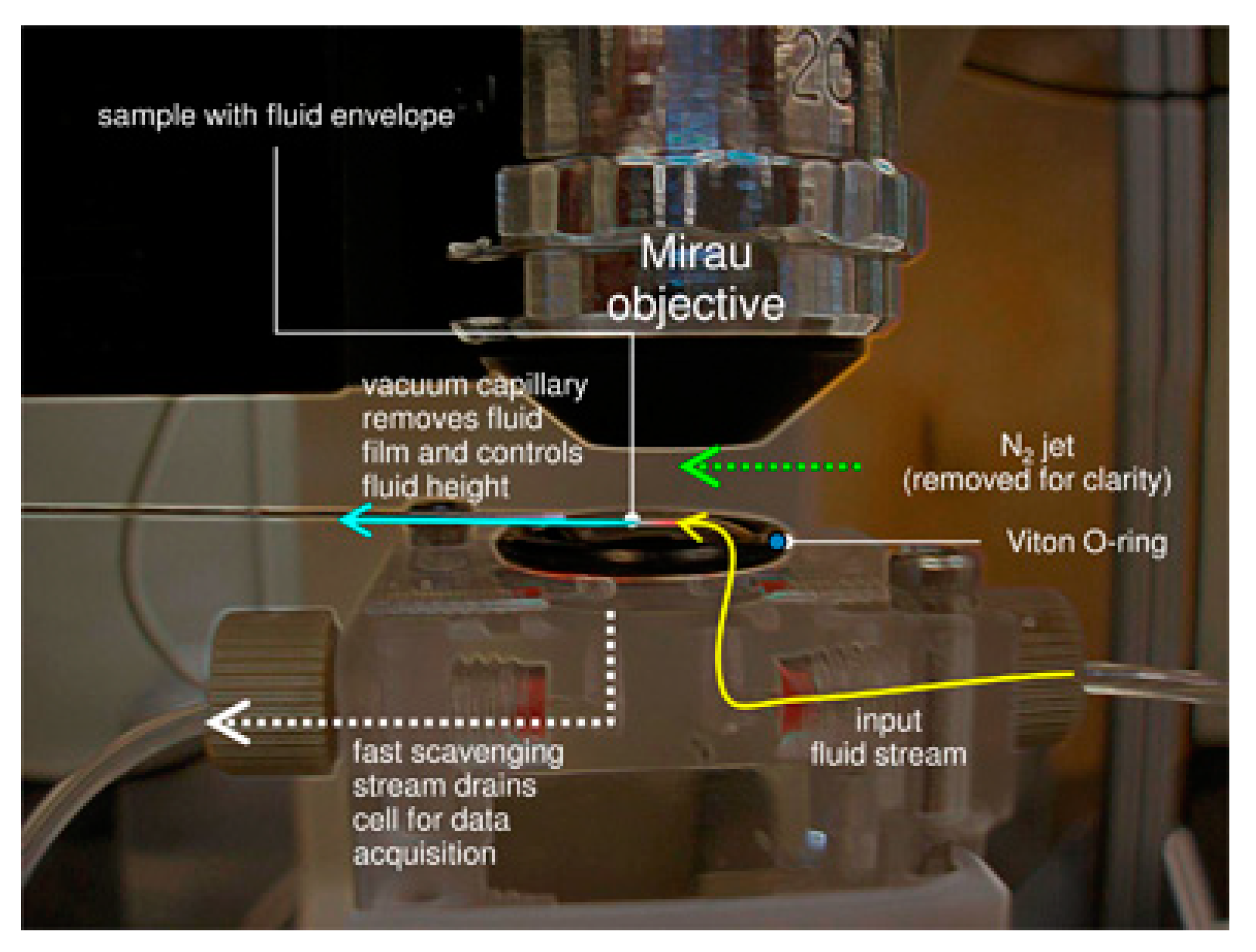
  146. Arvidson, R.S.; Luttge, A. System and method of fluid exposure and data acquisition. U.S. Patent US8164756B2, 29 September 2009. [Google Scholar]
  147. Luttge, A.; Arvidson, R.S. Reactions at surfaces: A new approach integrating interferometry and kinetic simulations. J. Am. Ceram. Soc. 2010, 93, 3519–3530. [Google Scholar] [CrossRef]
  148. Rubbo, M.; Bruno, M.; Massaro, F.R.; Aquilano, D. The five twin laws of gypsum (CaSO 4•2H 2O): A theoretical comparison of the interfaces of the penetration twins. Cryst. Growth Des. 2012, 12, 3018–3024. [Google Scholar] [CrossRef]
  149. García-Ruiz, J.M.; Villasuso, R.; Ayora, C.; Canals, A.; Otálora, F. Formation of natural gypsum megacrystals in Naica, Mexico. Geology 2007, 35, 327–330. [Google Scholar] [CrossRef] [Green Version]
  150. Pinto, A.J.; Ruiz-Agudo, E.; Putnis, C.V.; Putnis, A.; Jiménez, A.; Prieto, M. AFM study of the epitaxial growth of brushite (CaHPO4· 2H2O) on gypsum cleavage surfaces. Am. Mineral. 2010, 95, 1747–1757. [Google Scholar] [CrossRef]
  151. Massaro, F.R.; Rubbo, M.; Aquilano, D. Theoretical equilibrium morphology of gypsum (CaSO4· 2H2O).1.A syncretic strategy to calculate the morphology of crystals. Cryst. Growth Des. 2010, 10, 2870–2878. [Google Scholar] [CrossRef]
  152. Massaro, F.R.; Rubbo, M.; Aquilano, D. Theoretical equilibrium morphology of gypsum (CaSO4· 2H2O).2. The stepped faces of the main [001] zone. Cryst. Growth Des. 2011, 11, 1607–1614. [Google Scholar] [CrossRef]
  153. Rubbo, M.; Massaro, F.R.; Aquilano, D.; Vanzetti, W. Morphology of gypsum: A case study. Cryst. Res. Technol. 2011, 46, 779–783. [Google Scholar] [CrossRef]
  154. Rabizadeh, T.; Peacock, C.L.; Benning, L.G. Carboxylic acids: Effective inhibitors for calcium sulfate precipitation? Mineral. Mag. 2014, 78, 1465–1472. [Google Scholar] [CrossRef] [Green Version]
  155. Shukla, J.; Mehta, M.J.; Kumar, A. Solubility Behavior of Calcium Sulfate Dihydrate (Gypsum) in an Aqueous Sodium Chloride System in the Presence of Hydroxyalkyl Ammonium Acetate Ionic Liquids Additives: Morphology Changes and Physicochemical Solution Properties at 35 °C. J. Chem. Eng. Data 2019, 64, 5132–5141. [Google Scholar] [CrossRef]
  156. Cody, R.D.; Cody, A.M. Gypsum nucleation and crystal morphology in analog saline terrestrial environments. J. Sediment. Petrol. 1988, 58, 247–255. [Google Scholar] [CrossRef]
  157. Polat, S.; Sayan, P. Effect of various metal ions on gypsum precipitation. Indian Chem. Eng. 2020, 1–11. [Google Scholar] [CrossRef]
  158. Reiss, A.G.; Ganor, J.; Gavrieli, I. Size Distribution and Morphology of Gypsum Crystals Precipitating from Hypersaline Solutions. Cryst. Growth Des. 2019, 19, 6954–6962. [Google Scholar] [CrossRef]
  159. Montagnino, D.; Costa, E.; Massaro, F.R.; Artioli, G.; Aquilano, D. Growth morphology of gypsum in the presence of copolymers. Cryst. Res. Technol. 2011, 46, 1010–1018. [Google Scholar] [CrossRef]
  160. Hoang, T.A.; Ang, H.M.; Rohl, A.L. Effects of Organic Additives on Calcium Sulfate Scaling in Pipes. Aust. J. Chem. 2009, 62, 927. [Google Scholar] [CrossRef]
  161. Gránásy, L.; Pusztai, T.; Tegze, G.; Warren, J.A.; Douglas, J.F. Growth and form of spherulites. Phys. Rev. E Stat. Nonlinear Soft Matter Phys. 2005, 72, 011605. [Google Scholar] [CrossRef] [Green Version]
  162. Alimi, F.; Gadri, A. Kinetics and morphology of formed gypsum. Desalination 2004, 166, 427–434. [Google Scholar] [CrossRef]
  163. Andreassen, J.-P.; Lewis, A.E. Classical and Nonclassical Theories of Crystal Growth. In New Perspectives on Mineral Nucleation and Growth; Springer: Berlin, Germany, 2017. [Google Scholar]
  164. Stawski, T.M.; Freeman, H.M.; Van Driessche, A.E.S.; Hövelmann, J.; Besselink, R.; Wirth, R.; Benning, L.G. Particle-Mediated Nucleation Pathways Are Imprinted in the Internal Structure of Calcium Sulfate Single Crystals. Cryst. Growth Des. 2019, 19, 3714–3721. [Google Scholar] [CrossRef] [Green Version]
  165. Reiss, A.G.; Gavrieli, I.; Ganor, J. The Morphology of Gypsum Precipitated Under Hyper-saline Conditions – Preliminary Results from Dead Sea - Red Sea Mixtures. Procedia Earth Planet. Sci. 2017, 17, 376–379. [Google Scholar] [CrossRef]
  166. El-Shall, H.; Abdel-Aal, E.A.; Moudgil, B.M. Effect of surfactants on phosphogypsum crystallization and filtration during wet-process phosphoric acid production. Sep. Sci. Technol. 2000, 35, 395–410. [Google Scholar] [CrossRef]
  167. Reiss, A.G.; Ganor, J.; Hamawi, M.; Gavrieli, I. Dynamics of turbidity in gypsum-precipitating brines: the case of the Red Sea - Dead Sea project. 2021. Under review. [Google Scholar]
  168. Eberl, D.D.; Kile, D.E.; Drits, V.A. On geological interpretations of crystal size distributions: Constant vs. proportionate growth. Am. Mineral. 2002, 87, 1235–1241. [Google Scholar] [CrossRef]
  169. Middleton, G.V. Generation of the Log-Normal Frequency Distribution in Sediments. In Topics in Mathematical Geology; Springer: Berlin, Germany, 1970. [Google Scholar]
  170. Eberl, D.D.; Drits, V.A.; Środoń, J. Deducing growth mechanisms for minerals from the shapes of crystal size distributions. Am. J. Sci. 1998, 298, 499–533. [Google Scholar] [CrossRef]
  171. Koch, A.L. The logarithm in biology. J. Theor. Biol. 1969, 12, 276–290. [Google Scholar] [CrossRef]
  172. Crow, E.L.; Shimizu, K. Lognormal Distributions: Theory and Applications, 1 st ed.; Marcel Dekker: New York, NY, USA, 1987. [Google Scholar]
  173. Kile, D.E.; Eberl, D.D.; Hoch, A.R.; Reddy, M.M. An assessment of calcite crystal growth mechanisms based on crystal size distributions. Geochim. Cosmochim. Acta 2000, 64, 2937–2950. [Google Scholar] [CrossRef]
  174. Kile, D.E.; Eberl, D.D. On the origin of size-dependent and size-independent crystal growth: Influence of advection and diffusion. Am. Mineral. 2003, 88, 1514–1521. [Google Scholar] [CrossRef]
  175. Srodor, J.; Eberl, D.D.; Drits, V.A. Evolution of fundamental-particle size during illitization of smectite and implications for reaction mechanism. Clays Clay Miner. 2000, 48, 446–458. [Google Scholar] [CrossRef]
  176. Emmanuel, S.; Ague, J.J. Impact of nano-size weathering products on the dissolution rates of primary minerals. Chem. Geol. 2011, 282, 11–18. [Google Scholar] [CrossRef]
Figure 1. Experimentally-determined and calculated gypsum precipitation potentials from Dead Sea brine–seawater mixtures at T = 25 °C and P = 1 atm. The experimental data are derived from Reznik et al. [58]. Calculations are based on the two Pitzer.dat databases that were implemented in PHREEQC version 2.1 and 3.3. Figure reprinted from Rosenberg et al. [12] with permission of Elsevier.
Minerals 11 00141 g001
Figure 2. Measured gypsum solubility in 0–6 m NaCl solutions in temperatures ranging from 0.5 to 55 °C. Data points are all based on previous studies [67,68,69,70,71]. The line is based on thermodynamic calculations at 25 °C, while the dashed lines are the theoretical calculation ±3%. The calculations were performed with the Pitzer formalism and the parameterization of Harvie and Weare [46,51,57] as implemented in the Pitzer.dat database of PHREEQC version 2.18.
Minerals 11 00141 g002
Figure 3. The calculated solubility (a) and ratio of γSO42− (b), γCa2+ (c), and a 2 H 2 O (d) in pure water and in electrolyte solutions up to I = 6 m with Ca2+:SO42− = 1. Calculations were performed with Pitzer.dat database in PHREEQC 2.18. The ionic strength is derived from either NaCl (circles), KCl (triangles) or MgCl2 (squares) and does not include the contribution of the dissolved Ca2+ and SO42−.
Minerals 11 00141 g003
Figure 4. Calculated equilibrium concentration (eq.) of sulfate and calcium (m) in non-stoichiometric NaCl solutions (I = 3 m). If the ratio between the ions in solutions differs from that of the mineral, a relative larger amount of the less abundant ion would be incorporated into the mineral during precipitation. The ratio between the lattice ions at equilibrium is 0.45, 0.70, 1, 1.42, and 2.17. Note that for Ca2+/SO42− < 1 solubility is defined by the Ca2+ concentration whereas for Ca2+/SO42− > 1 solubility is defined by the SO42− concentration.
Minerals 11 00141 g004
Figure 5. Measured Log(Tind) for gypsum as a function of salinity in stoichiometric NaCl solutions at 25 °C and Ωgypsum = 3 vs. the calculated solubility of gypsum. Log(Tind) data points are from He et al. [77]; the calculated solubility data were calculated with the pitzer.dat database in PHREEQC 2.18 for 25 °C.
Minerals 11 00141 g005
Figure 6. Calculated log(Tind) for gypsum from seawater undergoing evaporation as a function of the evaporation factor, as calculated from Equation (7). The vertical and horizontal black lines are calculated log(Tind) at evaporation factors of 3.3 and 3.8 at which reportedly gypsum precipitates from seawater. Reprinted from Reznik et al. [79] with permission from Elsevier.
Minerals 11 00141 g006
Figure 7. Measured (points) and model calculated (lines) concentration of SO42− in mixtures of Dead Sea brine with either evaporated seawater (no inhibitor) or reject brine (scale inhibitor) as a function of time. The calculations are from a forward model based on Equation (9). (a) Seeded mixtures. (b) Unseeded mixtures. Note the one order of magnitude difference in the time scales of the two graphs. Although all four mixtures have the same initial oversaturation, the equations describing the seeded experiments (a) have two terms while in those describing the unseeded mixtures (b) kfar = 0, i.e., in effect Equation (9) is reduced back to Equation (8) which has only one term. The difference in the change in concentration of SO42− with time in the unseeded experiments is due to the antiscalant’s effect on the properties of gypsum formed during nucleation (see Reiss et al. [39]). Figure reprinted from Reiss et al. [39] with permission from Elsevier.
Minerals 11 00141 g007
Figure 8. Gypsum solubility (at 25 °C) and logarithm of rate coefficients for gypsum growth at a range of temperatures (25 °C, 50 °C, 70 °C, and 90 °C) in stoichiometric solutions as a function of salinity (0–6 m). Note that over the range of temperature presented, the rate coefficient increases and decreases with solubility. Rate coefficients are from He et al. [71]; solubility was calculated with PHREEQC (see also Figure 2).
Minerals 11 00141 g008
Figure 9. Change in the rate coefficient as a function of SO42− at equilibrium and Na+/Ca2+ activity ratio. Experimental data (dots) are derived from [71,110,137,139]. Calculations (lines) are based on Equation (11). Reprinted from Reznik et al. [110] with permission from Elsevier.
Minerals 11 00141 g009
Figure 10. Corrosion on the base of an atomic force microscopy (AFM) following contact with a mixture containing 70% wt. Dead Sea brine and 30% wt. seawater. The concentration of Cl in this mixture is about 3.86 m.
Minerals 11 00141 g010
Figure 11. Schematic representation of an in-situ flow-through growth experiment in the AFM. (a) Syringe pump injects solution into a flow-through cell thereby increasing the pressure within the cell, which may cause leaks. (b) Syringe pump draws the solution into the cell greatly reducing the chance of a leak.
Minerals 11 00141 g011
Figure 12. In-situ water–rock interaction apparatus. The crystal sample is placed within an O-ring under the objective of a vertical scanning interferometer (VSI). Inlet and outlet ports for the fluid are situated within the O-ring at opposite sides of the sample. Nitrogen (N2) gas jet is direct towards the outlet port. The whole apparatus is connected to a controller that is programmed to automatically run cycles in which the sample is submerged in a reactive solution for a predetermined time interval and then rapidly dried. The drying is performed by simultaneously activating the N2 jet, directed to push the solution towards the outlet port, and applying vacuum suction. The dried surface is then imaged. Figure reprinted from Luttge and Arvidson [147] with permission from Wiley.
Minerals 11 00141 g012
Figure 13. Halite cubes on the (010) surface of gypsum. The halite crystals precipitated from a solution originally undersaturated (Ωhalite ~ 0.1) with respect to the mineral.
Minerals 11 00141 g013
Figure 14. Common habits of gypsum. (a,b) selenite, (c) alabaster, and (d) satin spar. The diameter of the coin in the figure is 2.2 cm. Gypsum samples are from the Mineralogy and Petrology collection at the Institute of Earth Sciences, the Israeli National Natural History collections at the Hebrew University of Jerusalem.
Minerals 11 00141 g014
Figure 15. SEM images of individual gypsum crystals. While these crystals show different proportions between different surfaces (i.e., different morphology), they have all precipitated from the same brine (comprised of 85% wt. Dead Sea brine and 15% wt. seawater). Reprinted from Reiss et al. [158] with permission from the American Chemical Society.
Minerals 11 00141 g015
Figure 16. Gypsum crystals that precipitated from Dead Sea–seawater mixtures enriched with Ca2+ and SO42− to control oversaturation. (a,b) stellate crystals that precipitated from mixtures with Ωgypsum = 4. Blue line for scale is 100 µm and (c) crystals that precipitated from solutions with a Ωgypsum = 1.75.
Minerals 11 00141 g016
Figure 17. A plot of the measured LogTind vs. 1/log2(Ω) for different saline compositions. The Ωgypsum at which the slope changes is interpreted, based on the CNT as the oversaturation at which the mechanism of nucleation changes between homogeneous and heterogeneous. Series C–G represent different mixtures between Dead Sea brine and seawater. Reprinted From Reznik et al. [79] with permission from Elsevier.
Minerals 11 00141 g017
Figure 18. A lognormal crystal size distribution (CSD). CSD1 and CSD2 are the CSDs of two crystal populations that have precipitated from a Ca2+ and SO42− enriched mixture of 85% wt. Dead Sea brine and 15% wt. seawater. The data are reprinted from Reiss et al. [158] with permission from the American Chemical Society.
Minerals 11 00141 g018
Publisher’s Note: MDPI stays neutral with regard to jurisdictional claims in published maps and institutional affiliations.

