The Surface-Vacancy Model—A General Theory of the Dissolution of Minerals and Salts

Abstract

The kinetics of the dissolution of salts and minerals remains a field of active research because these reactions are important to many fields, such as geochemistry, extractive metallurgy, corrosion, biomaterials, dentistry, and dietary uptake. A novel model, referred to as the surface-vacancy model, has been proposed by the author as a general mechanism for the primary events in dissolution. This paper expands on the underlying physical model while serving as an update on current progress with the application of the model. This underlying physical model envisages that cations and anions depart separately from the surface leaving a surface vacancy of charge opposite to that of the departing ion on the surface. This results in an excess surface charge, which in turn affects the rate of departing ions. Thus, a feedback mechanism is established in which the departing of ions creates excess surface charge, and this net surface charge, in turn, affects the rate of departure. This model accounts for the orders of reaction, the equilibrium conditions, the acceleration or deceleration of rate in the initial phase and the surface charge. The surface-vacancy model can also account for the effect of impurities in the solution, while it predicts phenomena, such as ‘partial equilibrium’, that are not contemplated by other models. The underlying physical model can be independently verified, for example, by measurements of the surface charge. This underlying physical model has implications for fields beyond dissolution studies.

1. Introduction

Dissolution of minerals and salts is one of the most important reactions in chemistry. Because it is possibly the oldest known class of reactions, dissolution is known by different names in a wide range of fields—dissociation, digestion, etching, corrosion, leaching, weathering, and decay are some examples. Despite the obvious importance of this reaction, there is no generally accepted theory of the mechanism of dissolution that accounts for various experimental observations. Recently, the author has proposed a novel theory based on the ionic charging of the surface [1,2,3,4,5,6]. This theory has been shown to describe the kinetic observations for a diverse range of minerals, including quartz and silica (SiO₂) [7], salt (NaCl) [8], forsterite (Mg₂SiO₄) and the olivine group [9], feldspars (KAlSi₃O₈, NaAlSi₃O₈, CaAl₂Si₂O₈) [10,11], oxide minerals [3] and silicate minerals [2]. The purpose of this paper is to provide an exposition of this theory with specific focus on the underlying physical model, showing that the model describes the principal features of dissolution reactions.

Kinetic models proposed for dissolution reactions have generally been unsuccessful in three major areas: (i) the orders of reaction with respect to the concentrations of reactant in solution, mostly importantly H⁺ and OH⁻ ions; (ii) the acceleration or deceleration in the initial rate of reaction; (iii) the development of surface charge during dissolution or crystallization.

The first of these principal difficulties in understanding the mechanism of dissolution is that the kinetics exhibit fractional orders of reaction. Frequently, they are close to one-half. Considering that dissolution reactions are chemically quite simple, for example, $ZnO+2H^{+}\to Z{n}^{2+}+H_{2}O$, the fact that the rate is proportional to the concentration of H⁺ to the power of 0.5 indicates that these simple reactions are not elementary reactions. As the minimum stoichiometric number in an elementary reaction is one, it is difficult to derive values for orders of reaction below one, such as those found in many dissolution reactions, using multistep mechanisms. That the order of reaction is fractional points to a depth to dissolution reactions that is not easily explained.

The second principal difficulty in the understanding of the mechanism of dissolution is the observation that the initial rate of dissolution is sometimes accelerating and at other times decelerating. In other words, the initial rate per unit area under some conditions is initially fast and then slows to a steady value. Conversely, under other conditions, the rate of the reaction starts slowly, and accelerates to a constant value [12]. This points to a change in a property of the surface that is initially away from and then moves towards a stationary value. None of the current models of the dissolution clearly account for this phenomenon.

The third principal difficulty in the understanding of the mechanism of dissolution is the observation that the surfaces of salts and minerals are electrically charged. For minerals such as oxides and clays, this property is well-known, and mechanisms, such as H⁺ adsorption for oxides and ion-exchange for clays, have been proposed to account for this charge.

More importantly, what is generally not recognized in the dissolution literature is that the surfaces of salts in aqueous solution are also electrically charged [8,13]. The explanation of charge on the surface of salts is not possible by an explanation of proton absorption, surface complexation or ion exchange because there are no foreign ions in solution. This means that there is a mechanism for the formation of surface charge on solids that is not dependent on mechanisms of adsorption of foreign ions.

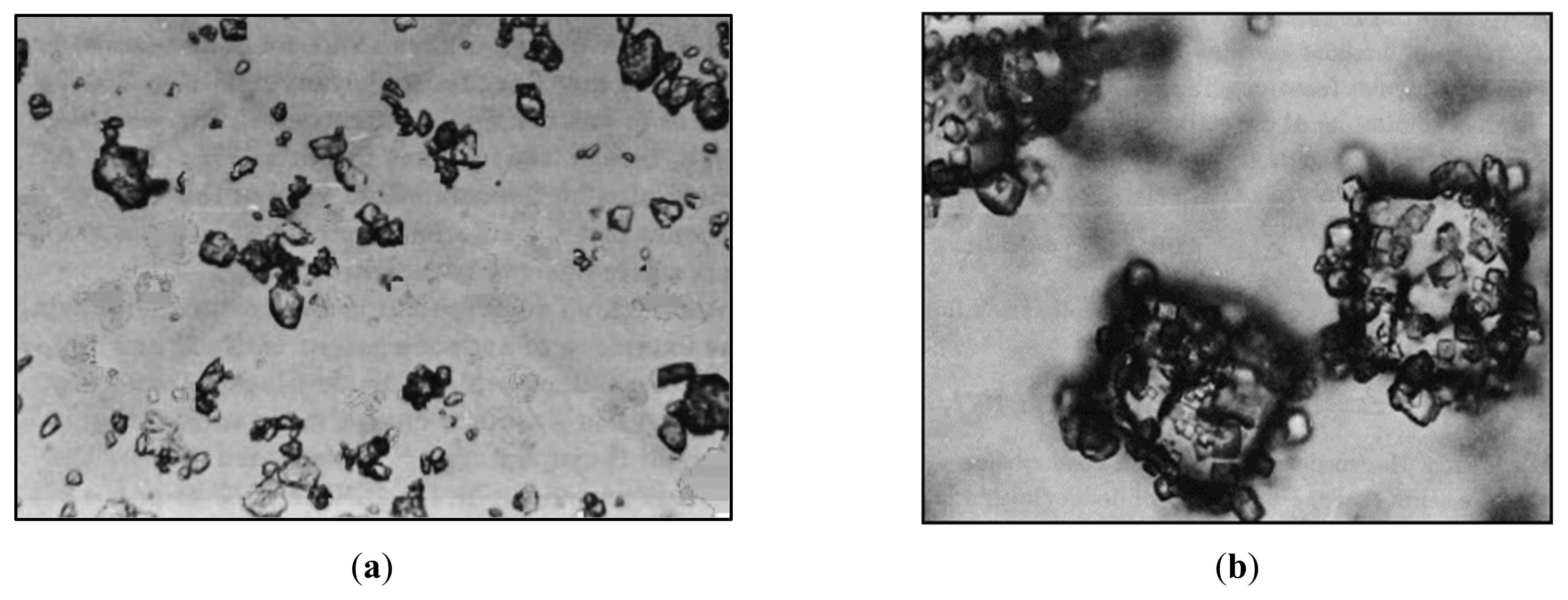
A micrograph is shown in Figure 1 in which smaller KCl particles are attracted to the surfaces of larger NaCl particles because of their opposite charges. As a result, the smaller KCl particles cling to the larger NaCl particles.

The charge on the surface of salt has been determined by a variety of techniques, including membrane potentiometry and electrophoresis [14,15,16,17]. Industrially, the opposite charges on the surfaces of NaCl and KCl are exploited in the flotation of potash, where a positively charged collector attaches to a negatively charged surface and induces a flotation response [14].

It is essential that the effect of the surface charge is coherently incorporated into the mechanism of dissolution because dissolution is the removal of charged particles from the surface and the presence of a net surface charge should affect the rate at which these particles are removed. It is argued in this paper that the surface charge is a ‘hidden variable’ in dissolution and crystallization kinetics. It is the key that unlocks the understanding of the mechanism of dissolution.

Two broad approaches to developing a fundamental mechanism of dissolution have been developed in the past. The first approach is to build a molecular model, for example, in which bonding atoms are removed according to their coordination with other members of the constituent solid. This approach has been pursued several times over the last few decades [18,19,20]. However, this approach has only partially addressed the orders of reaction and has not addressed surface charge.

The second approach to developing a fundamental understanding of the kinetics of dissolution is the testing of kinetic mechanisms. In this approach, a mechanism is first proposed, then a rate law is derived from the proposed mechanism, and finally this rate law is compared with the experimental results. Before this approach is discussed, it is worth considering the experimental results that are used in the verification of the mechanism.

The experimental measurements are the effects of temperature and concentration on the rate of reaction, which can be summarized as an empirical expression of the form $rate=-k{\left[C\right]}^n\exp \left\{-\frac{E_A}{RT}\right\},$ where $\left[C\right]$ represents the concentration of $C$ in solution, $n$ represents the order of reaction with respect to the species with concentration $C$, and $E_A$ is the activation energy. The other symbols $R$ and $T$ represent the gas constant (8.314 J·K⁻¹·mol⁻¹) and the absolute temperature (K). The rate is usually expressed in mol·m⁻²·s⁻¹, but an alternative unit that is used in fields such as corrosion is m·s⁻¹. The former unit divided by the molar density of the solid yields the latter. The key experimental results are the orders of reaction, $n$, with respect to each of the reactants, and the activation energy. These parameters quantify the effects of concentration and temperature.

A mechanism in chemical kinetics is a set of elementary reaction steps. By elementary steps, it is meant that the order of reaction reflects the molecularity of the reaction step. Thus, if the step $2A+3B\to A_2{B}_3$ is an elementary step, the requirement is that the rate of reaction is proportional to the probability of a collision of two molecules of $A$ and three molecules of $B$, which means the rate expression is $rate=-k{\left[A\right]}^2{\left[B\right]}^3$, where the order of reaction is 2 with respect to $A$ and 3 with respect to $B$ [21]. Importantly, this means that the stoichiometric coefficients in an elementary step cannot be fractions. Thus, this approach requires the proposal of elementary reaction steps with integer-valued stoichiometry whose individual rate expressions combine so that the orders of reaction derived for the overall reaction agree with those obtained experimentally. Expressed differently, the orders of reaction provide researchers with a macroscopic window to the microscopic events occurring during reaction.

The rate of dissolution of solids varies over many orders of magnitude. For some solids, this rate is sufficiently fast that the overall rate is controlled by diffusion within the hydrodynamic boundary layer. In this study, we exclude data in which such film diffusion is rate-controlling because the focus is on the kinetics of the chemical reaction at the surface. In addition, diffusional processes to a planar non-porous surface are described by Fick’s law, $rate=-D dC/dx,$ which in an integrated form for diffusion control is $rate=-D/\delta \left(C\right)$. Clearly, this expression is first order with respect to the diffusing species. Diffusion alone cannot explain orders of reaction that are not equal to one.

Several proposals for mechanisms of reaction have been made for dissolution. The first proposal is referred to as the surface-complexation model, which proposes that a ‘complex’ forms on the surface between the reactant and the surface species, and that it is the departing of this complex that is this rate limiting step [22,23,24]. The rate of reaction is given by the expression $rate=-k{[>ML]}^p$, where $[>ML]$ is the concentration of the surface complex, and $p$ is the order of reaction. The concentration of $[>ML]$ is not measured; rather, it is calculated by proposing multiple equilibria involving solution species and hypothetical surface species. Although Casey [25] proposed an explanation for $p$, the underlying model introduces numerous adjustable parameters that have not been independently verified. In effect, the model creates a new order of reaction and ignores the fractional orders with respect to solution species.

An alternative proposal for the mechanism of dissolution is the precursor-species model, in which a precursor forms on the surface that then reacts to form an ‘activated complex’, which in turn decomposes to form the reaction products [26,27,28,29]. However, the proponents of this model make the mistake of using fractional stoichiometry to obtain fractional orders of reaction, which, as explained earlier, makes no sense in the context of kinetic mechanisms composed of elementary reactions.

Yet another proposed mechanism of dissolution uses crystallization theory [30]. Rate expressions based on degree of saturation have been derived from crystal growth theories of the terrace-edge-kink type [30]. These models are concerned mainly with the approach to equilibrium, and do not address any of the three challenges of dissolution reactions that are the subject of this paper, namely, fractional orders of reaction, accelerating or decelerating initial rates, and surface charge.

Thus, the current models of dissolution are deficient because they cannot explain (i) reaction orders, (ii) initial transients, and especially (iii) surface charge. The purpose of this paper is to provide a general theory of dissolution that accounts for these experimental observations in a holist manner. The objectives of the present work and the requirements for a general dissolution model are presented in the next section. Following this, the underlying physical foundations of the proposed model are described. From this physical model, kinetics expressions are derived. The correspondence between the model and the experimental data for the different observed parameters, such as the reaction orders, and phenomena, such as transient effects, is discussed. The implications of the model are discussed, and suggestions for independent testing are made.

2. Objectives of This Paper

The aim of this work is to outline a general model of the dissolution of salts and minerals. As discussed in the introduction, the most important requirements for a general model of dissolution are as follows:

• It should be applicable to the (non-oxidative) dissolution of all minerals and salts.
• It must provide a clear physical foundation from which the rate equations are derived.
• It must coherently describe the effect of surface charge on the rate of removal of ions.
• The rate expressions derived from the physical model must inherently and coherently describe the following dissolution phenomena:

  (a)

  The effects of H⁺ and OH⁻ on the rate of dissolution expressed in terms of the order of reaction with respect to these reactants;

  (b)

  The approach to equilibrium, including the effects of constituent ions in solution on the rate of dissolution, for example, Na⁺ on the rate of dissolution of NaCl;

  (c)

  The change in rate of dissolution, either acceleration or deceleration, during the initial stage of reaction;

  (d)

  The non-stoichiometric dissolution of more complex solids, such as felspars.

• The physical foundations of the model should be testable by independent means.
• The model should make predictions that extend the field.

The surface-vacancy model is the only model that meets these requirements. (In previous papers, the author referred to this model as the surface-dissociation model, but the name surface-vacancy model is preferred because it better reflects the underlying physical features of the model.) The physical foundations of this model are laid down in the next section. In the sections that follow this foundational material, it is shown that the surface-vacancy model describes the orders of reaction with respect to H⁺ and OH⁻, that it describes the approach to equilibrium, that it describes the change in initial rate of dissolution, and that it describes the non-stoichiometric phases of dissolution. Importantly, the physical model provides predictions that allow the model to be independently and more thoroughly tested. Finally, and by no means least, are the predictions that the model makes that are not made by other models, and which allow the field to develop further.

As mentioned, the next section lays down the physical foundations of this model.

3. Physical Foundations of the Surface-Vacancy Model of Dissolution

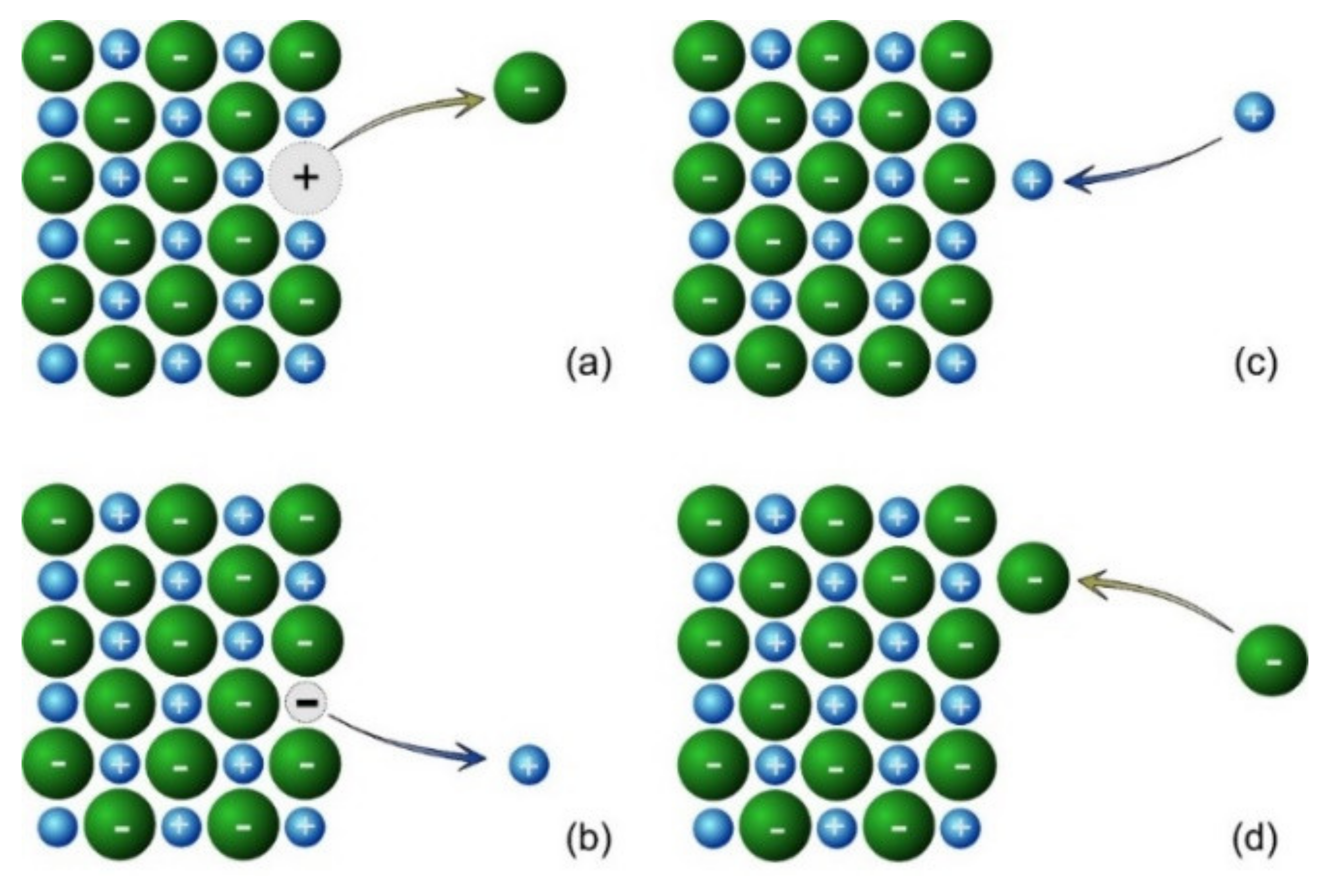
When ions depart from the surface to dissolve in the aqueous phase, they leave a vacancy of equal charge but of opposite sign to the ion. This results in a net excess charge on the surface, shown in Figure 2a,b. Of course, the deposition of ions from the aqueous solution can also occur, also resulting in excess charge, as shown in Figure 2c,d. Therefore, there are four events that must be considered in the kinetic model.

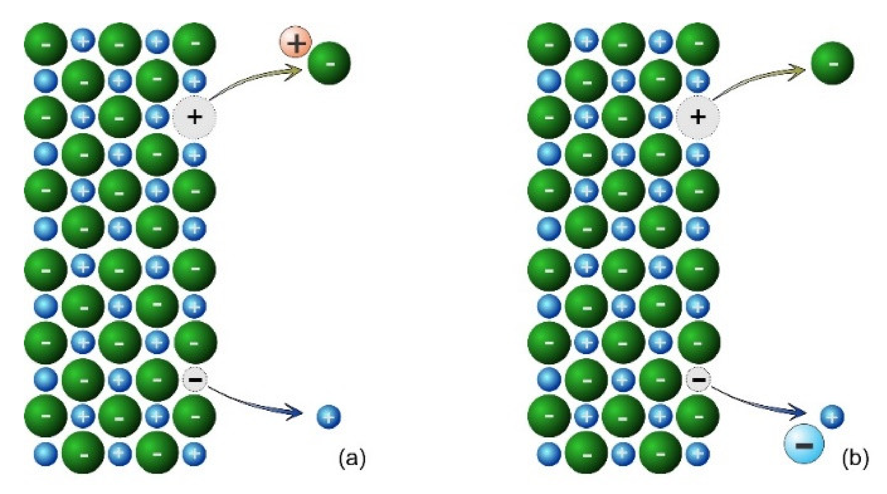
This situation describes the underlying physical model for salts, where the dissolution is an interaction between the solid and the solvent. For other minerals, the rate of dissolution is enhanced in either acid or alkaline solutions or both, so the physical model must be extended to include H⁺ and OH⁻. In this case, the underlying physical model is shown in Figure 3. The removal of the anion from the surface occurs with the participation of a proton (or hydronium ion), shown in Figure 3a. Likewise, the removal of the cation from the surface occurs with the participation of the hydroxide ion, shown in Figure 3b. The impact of ligands occurs in a similar manner—anionic ligands assist in the removal of cations from the surface, leaving a negative vacancy, while cationic ligands assist in the removal of anions from the surface, leaving a positive vacancy.

Consider the dissolution of a solid $MA$ in acid according to the reaction (1). Furthermore, consider for the sake of simplicity only the forward reaction.

$$MA+t{H}^{+}\to M^{+}\left(aq\right)+H_t{A}^{t-1}$$

(1)

The symbol $t$ represents the stoichiometric coefficient for the number of protons (hydronium ions) that interact with the anion during its removal from the surface. The values of $t$ are restricted to 0, 1, 2, 3…$n$.

The individual steps corresponding to Figure 2a,b can be expressed in chemical notation as Equations (2) and (3), where $\equiv M$ and $\equiv A$ represent the M-constituent and the A-constituent of the solid surface, respectively. Likewise, ${\equiv }^{+}$ represents a surface vacancy with a positive charge, and ${\equiv }^{-}$ represents a vacancy with a negative charge.

$$\equiv M \to M^{+}\left(aq\right)+{\equiv }^{-}$$

(2)

$$\equiv A+t{H}^{+}\to H_t A^{t-1}\left(aq\right)+{\equiv }^{+}$$

(3)

The formulation is not restricted to minerals with 1:1 stoichiometric ratio—the reaction scheme can be extended to any stoichiometry.

If dissolution occurs in an alkaline medium by, for example, $MA+sO{H}^{-}\to M{\left(OH\right)}_s^{1-s}\left(aq\right)+{\mathrm{A}}^{-}\left(aq\right)$, the dissolution steps are given by Equations (4) and (5).

$$\equiv M+sO{H}^{-}\to M{\left(OH\right)}_s^{1-s}\left(aq\right)+{\equiv }^{-}$$

(4)

$$\equiv A\to A^{-}\left(aq\right)+{\equiv }^{+}$$

(5)

Other extensions to these simple steps might be envisaged. For example, a similar scheme can be envisaged to account for ligand interactions. In electrochemical kinetics, it is often postulated that the first step is the adsorption of an ion, say a proton or a ligand, onto the surface before the rate-determining step. This might allow for a saturation effect of the ion by applying an isotherm, for example, the Langmuir isotherm. Such additional or prior steps can be incorporated.

Due to the removal of ions from the surface, there is a net charge on the surface. This net charge affects the affects the rate at which ions are removed. Thus, this forms a feedback mechanism: removal of ions causes a charge, but this charge affects the rate of removal. This means that the individual steps shown in Equations (2)–(5) are not chemical, but electrochemical.

To summarize, the physical foundations of the proposed model of dissolution are (i) the removal of ions creates a vacancy of charge opposite that of the departing ion on the surface, (ii) the removal of ions leaves a net excess charge on the surface, (iii) the net excess charge has a strong influence on the rate of removal of ions, and (iv) the rate of removal of ions might be enhanced by H⁺, OH⁻ or some other ligand.

Questions that may come to mind from this formulation of dissolution might include, amongst others, the following: (a) If the rate of removal of anions and cations are independent, what principle determines that the rate of removal of anions is stoichiometrically equivalent to the rate of removal of cations? (b) What principle governs steady state dissolution? (c) Is this consistent with chemical thermodynamics? These questions are answered in the next section in which this physical foundation is transformed into mathematical expressions for the surface charge and for the rate of dissolution.

4. Mathematical Formulation of the Surface-Vacancy Model

The excess surface charge at any time is the difference in surface concentration of the vacancies and deposited ions on the surface, given by Equation (6). The surface charge is given by ${\sigma }_0$, and the symbols $n_a$ and $n_c$ represent the surface concentrations of the anionic and cationic vacancies, respectively. The symbols ${\nu }_a$ and ${\nu }_c$ represent the absolute charge number of the anion and cation, respectively, so that for 1:1 salts such as NaCl, ${\nu }_a={\nu }_c=1$. $F$ represents the Faraday constant (C·mol⁻¹).

$${\sigma }_0=F\left({\nu }_c{n}_c-{\nu }_a{n}_a\right)$$

(6)

Equation (6) can be written as the difference in excess anions and cations using the symbols ${\Gamma }_{-}$ and ${\Gamma }_{+}$ [31]. The symbol $n$ is specifically used here to emphasize that the mechanism of surface charging is by surface vacancies and deposition.

Taking derivatives with respect to time, Equation (6) can be written as Equation (7).

$$\frac{d{\sigma }_0}{dt}=F\left({\nu }_c\frac{d{n}_c}{dt}-{\nu }_a\frac{d{n}_a}{dt}\right)$$

(7)

The rate of change of the surface concentration of cationic vacancies is equal to the rate of removal of anionic species, that is, $d{n}_c/dt$ is equal to $r_{-}$, and similarly, $d{n}_a/dt$ is equal to $r_{+}$. Since the charge number of the departing ion is the absolute value of the vacancy left behind, ${\nu }_a$ is the same as ${\nu }_{+},$ and ${\nu }_c$ is the same as ${\nu }_{-}$. The substitution of these relationships into Equation (7) yields Equation (8).

$$\frac{d{\sigma }_0}{dt}=F\left({\nu }_{-}{r}_{-}-{\nu }_{+}{r}_{+}\right)$$

(8)

Equation (8) relates the change in the electrical conditions of the surface to the dissolution kinetics. If the rate of removal of the cations is not in stoichiometric proportion to the rate of removal of anions, the surface charge will change with time according to Equation (8). Therefore, Equation (8) encapsulates the cause of transient effects: the surface charge is yet to reach its stationary state, and changes in the rate of removal of anions and cations will be experienced until a stationary state is reached. This expression will be revisited when the transient effects are discussed later.

Assume for the time being that a stationary state has been reached, so that the left-hand side of Equation (8) is approximately zero. This then yields Equation (9), which is a statement of stoichiometry.

$${\nu }_{-}{r}_{-}={\nu }_{+}{r}_{+}$$

(9)

This result is crucial—Equation (9) states that the condition for stoichiometric dissolution is that the surface charge is stationary, and that dissolution occurs at a constant rate, while Equation (8) describes the path that is taken to reach this stationary state where stoichiometric dissolution takes place.

In addition, Equation (8) describes how the individual steps of Equations (2) and (3) are linked to the overall reaction. The connection is not through chemistry, nor with a surface with neutral charge (which is the tacit assumption of all previous models of dissolution and crystallization), but through the surface charge reaching a stationary state. There are, in fact, three obvious stationary states: (i) dissolution at a constant rate; (ii) equilibrium, in which the rates of dissolution are matched by the rates of crystallization; (iii) crystallization at a constant rate.

Consider for the sake of presentation, that the dissolution reaction is given by Equation (1). As mentioned previously, the rates of removal of the anions and cations must be affected by the surface charge. In electrochemistry, this dependence is expressed in the form of a Boltzmann-like function with the potential difference across the Helmholtz layer as the independent variable [32]. If a double layer is assumed, then the surface charge and the potential difference are proportional to each other, with the constant of proportionality referred to as the surface capacity. This means that the rate of the removal of cations (Equation (2)) is given by Equation (10), and the rate of removal of anions, Equation (3), is given by Equation (11).

$$r_{+}={\overrightarrow{k}}_{+}exp\left(y\right)$$

(10)

$$r_{-}={\overrightarrow{k}}_{-}{[H^{+}]}^{t}exp\left(-y\right)$$

(11)

The symbols ${\overrightarrow{k}}_{-}$ and ${\overrightarrow{k}}_{+}$ represent the rate constants for the removal of anions and cations, respectively. The symbol y represents the dimensionless factor $0.5F\Delta \varphi /RT$, which includes the surface potential difference, $\Delta \varphi$. The terms $exp\left(y\right)$ and $exp\left(-y\right)$ are the Boltzmann-like factors that account for the effect of surface potential on the rate. This effect arises from the effect of potential on the activation barrier, identical to those found in electrochemical reactions. The factor 0.5 arises because the activated state (transition state) occurs approximately halfway between the surface and the outer Helmholtz plane [32].

Equations (9)–(11) represent three equations in the three unknowns, $r_{+}$, $r_{-}$ and $y$, which can be easily solved by substituting both Equations (10) and (11) in Equation (9), and making $y$ the subject of the formula. This operation yields Equation (12).

$$\mathit{exp}\left(2y\right)=\frac{{\overrightarrow{k}}_{-}{[H^{+}]}^t}{{\overrightarrow{k}}_{+}}$$

(12)

Equation (12) describes the effect of pH on the potential difference across the Helmholtz double layer, which can be determined by zeta potential and other electrochemical techniques.

The rate of dissolution is obtained by substituting Equation (12) into either Equation (10) or (11), which yields Equation (13).

$$rate={\left({\overrightarrow{k}}_{+}{\overrightarrow{k}}_{-}\right)}^{1/2}{[H^{+}]}^{t/2}$$

(13)

Thus, Equation (13) represents the simplest rate expression derived from the physical foundations presented in the previous section. Only dissolution due to acid, at steady conditions of dissolution, and at conditions far from equilibrium have been considered. Of course, these other cases can be accounted for, some of which will be addressed later in this paper, but Equation (13) combines the main features of the physical foundations into its simplest form so that it can be tested.

The significance of Equation (13) is that it predicts that if one proton is involved in the elementary step given by Equation (3), then $t=1$, and the order of reaction $t/2$ is equal to one-half. This demonstrates that the surface vacancy model correctly predicts one of the most difficult aspects of dissolution reactions.

Furthermore, the values of $t$ in Equation (13) take on values of 0, 1, 2, 3,…$t$, which means that the order of reaction with respect to H⁺ can take on values of 0, 0.5, 1.0, 1.5,…$t/2$. If a salt dissolves without the assistance of acid or alkali, the value of $t$ is zero, and the order of reaction is zero.

From kinetic theory, the formation of an activated complex becomes less likely as the number of species forming the activated complex increases. This means that the likelihood of finding minerals with an order of reaction of 0.5 is greater (because only one proton is involved) than finding those with an order of reaction of 1.0 (where two protons are involved), etc., and so forth.

This means that the expectation from the surface-vacancy model is that values of about one-half will be encountered most frequently. Values of one are expected less frequently than values of one-half, and values of one-and-a-half are expected at lower than this. This prediction of the orders of reaction is examined in the next section.

5. Testing the Surface-Vacancy Model—Orders of Reaction

Generally, the approach in dissolution studies is to focus on a single mineral reaction and examine its behavior in detail. Specific applications of the surface-vacancy model have been made for silica and quartz [2,7], feldspars [10,11], forsterite [9], oxides [3] and halite [8].

However, a broad approach is required for testing a general model such as the surface-vacancy model, and this broad approach is adopted in this paper. In this section, the predictions of the model are tested against data for the orders of reaction for metal oxides, orthosilicates and metal sulphides. Following this, the scenario of equilibrium is considered, after which the phenomenon of decelerating and accelerating dissolutions rates is analyzed.

5.1. Overview of Orders of Reaction

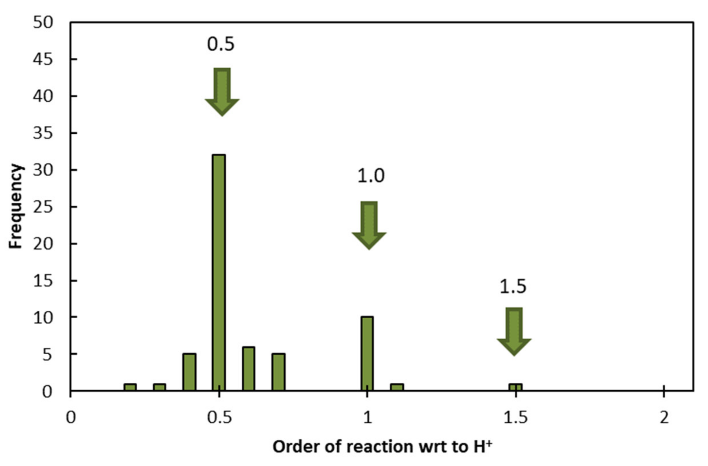
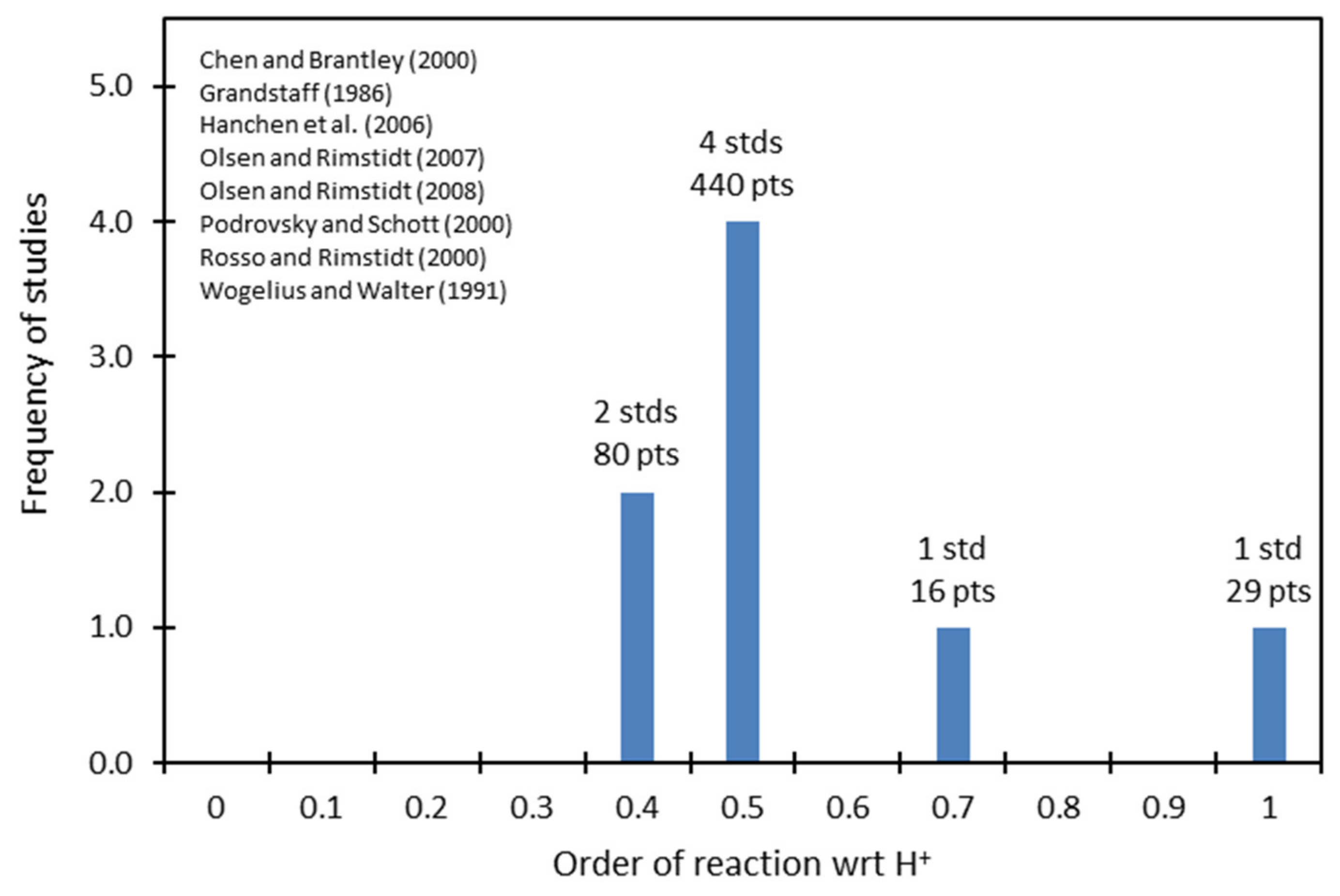
The orders of reaction with respect to H⁺ reported by 62 independent studies of different minerals are shown in Figure 4. These results suggest the clustering of the data about 0.5, at 1.0 with a lower frequency, and at 1.5 with an even lower frequency. These results agree with the surface-vacancy model presented in the previous section: as $t$ in Equation (13) takes on values of 0, 1, 2, 3,…$t$, the order of reaction with respect to H⁺ takes on values of 0, 0.5, 1.0, 1.5,…$t/2$, with diminishing frequency. No previously proposed model has been able to derive a relationship of this nature, and these results provide a powerful indication of the validity of the surface-vacancy model.

There is scatter of the data about these values, particularly around the value of 0.5. Such scatter is expected due to random experimental errors. For example, shown in Figure 5 are the frequencies of reported values for the order of reaction with respect to H+ for forsterite, Mg₂SiO₄, in the acidic region. This figure indicates that although six studies reported values close to 0.5, two were significantly distant from this value. As the number of data points (tests of the rate of dissolution) accumulate, so the confidence increases in the reported value. Thus, the value for forsterite 520 tests attested to a value close to 0.5, while 45 tests suggest a significant deviation from this value.

The results shown in Figure 4 correspond with the predictions of Equation (13), the simplest form of the surface-vacancy model. As mentioned in the previous section, one would expect from kinetic theory that the frequency of a value of one for $t$ would be higher than a value of 2, and that of two would be higher than that of 3, etc. This means that it is expected that the frequency of the order of reaction with respect to H+ of 0.5 would higher than 1.0, which in turn would be higher than that of 1.5. (This is subject to the obvious proviso that the measurements are obtained under conditions that are controlled by reaction kinetics and are not under diffusional control or mixed control.)

5.2. Orders of Reaction for Mineral Oxides

Consider the dissolution of a mineral oxide in an acidic aqueous solution for the conditions of steady-state dissolution at conditions far from equilibrium. The orders of reaction for mineral oxides under these conditions are given in

Table 1. Orders of reaction with respect to H⁺ for the dissolution of metal oxides.

Mineral Formula	Solution	Reaction Order with Respect to H+	Reference
γ-Al(OH)3	HNO3	1.0	[39]
δ-Al2O3	HNO3	0.41	[23]
λ-Al(OH)3	HNO3	1.5	[39]
BeO	HCl	0.49	[40,41]
BeO	H2SO4	0.49	[40,41]
BeO	H2C2O4	0.57	[40,41]
CoO	H2SO4	0.5	[42]
Cr2O3	HClO4	0.46	[43]
Cr(OH)3	HCl	0.46	[44]
CuO	H2SO4	0.5	[45]
CuO	HClO4	1.0	[45]
CuO	HNO3	1.0	[45]
CuO	HCl	1.0	[45]
Fe2O3	HCl	0.5	[43]
Fe2O3	H2SO4	0.5	[43]
Fe2O3	HNO3	0.5	[43]
Fe2O3	HClO4	0.5	[43]
α-FeOOH	HNO3	0.33	[19]
Fe(OH)3	HClO4	0.48	[46]
MgO	HNO3	0.49	[47,48,49]
Mg(OH)2	HCl	0.47	[48,49]
MnO	H2SO4	0.5	[43]
NiO	H2SO4	1.0	[48]
Ni2O3	H2SO4	0.5	[43]
UO3	H2SO4	0.5	[50]
V2O3	HClO4	0.5	[43]
ZnO	HCl	0.55	[51,52,53]
ZnO	HClO4	0.67	[49,53]
ZnFe2O4	H2SO4	0.6	[49,53]
ZnFe2O4	H2SO4	0.5	[54]
ZnFe2O4	HCl	0.5	[43]

. Many of the orders of reaction with respect to H⁺ are close to 0.5, while fewer are close to 1.0, and only one has a value close to 1.5.

5.3. Orders of Reaction for Orthosilicates

The orders of reaction for orthosilicates are given in

Table 2. Orders of reaction with respect to H⁺ for the dissolution for the orthosilicate minerals.

Mineral Formula	Mineral	Structure	Reaction Order with Respect to H+	Solution	Reference
Be2SiO4	Phenakite	Phenakite	0.3	HCl	[55,56]
CaMgSiO4	Monticellite	Olivine	0.56	HCl	[56]
Ca2SiO4	Ca-olivine	Olivine	0.42	HCl	[56]
Co2SiO4	Co-olivine	Olivine	0.36	HCl	[56]
CoMnSiO4	Co-Mn olivine	Olivine	0.42	HCl	[56]
Fe2SiO4	Fayalite	Olivine	0.69	HCl	[38,57]
Mg2SiO4	Forsterite	Olivine	0.45 to 0.54	HCl	[56,58,59]
Mn2SiO4	Tephroite	Olivine	0.47	HCl	[56,60]
Zn2SiO4	Willemite	Phenakite	0.45	HCl	[53]
Zn2SiO4	Willemite	Phenakite	0.49	H3PO4	[53]
Zn2SiO4	Willemite	Phenakite	0.53	H2SO4	[53]
Zn2SiO4	Willemite	Phenakite	0.38	HNO3	[53]
Zn2SiO4	Willemite	Phenakite	0.40	HClO4	[53]

. All the reported values are close to 0.5, in agreement with the surface-vacancy model.

5.4. Orders of Reaction for Feldspars

The orders of reaction with respect to H⁺ for feldspars are given in

Table 3. Orders of reaction for the dissolution of the feldspars at 25 °C.

Mineral Formula	Mineral	Reaction Order with Respect to H+	Reference
KAlSi3O8	K-feldspar	0.5	[57,58,61]
NaAlSi3O8	Albite	0.40 to 0.46	[58,61]
Na0.8Ca0.2Al1.2Si2.8O8	Oligoclase	0.46	[57,58,61]
Na0.6Ca0.4Al1.4Si2.6O8	Andesine	0.54	[57,58,61]
Na0.4Ca0.6Al1.6Si2.4O8	Labradorite	0.63	[57,58,61]
Na0.2Ca0.8Al1.8Si2.2O8	Bytownite	1.02	[57,58,61]
CaAl2Si2O8	Anorthite	1.4 to 1.5	[57,58,61]

. All these values are close to 0.5, except for bytownite and anorthite, which have values of 1.0 and 1.5. These values are in agreement with the surface-vacancy model.

5.5. Orders of Reaction for Metal Sulphides

The values reported for the order of reaction with respect to H⁺ for some metal sulphides are given in

Table 4. Orders of reaction with respect to H⁺, H₂S and M²⁺ for the dissolution of metal sulphides.

Mineral Formula	Solution	Reaction Order with Respect to H+ for Forward Reaction	Reaction Order with Respect to H2S for Reverse Reaction	Reaction Order with Respect M2+ for Reverse Reaction	Reference
CdS	H2SO4	0.99	0.48	0.49	[62]
FeS	HClO4	0.5	-	-	[63,64]
Ni1.54S	HCl	0.5	-	-	[65]
Ni0.45S	HCl	0.5	-	-	[65]
PbS	HClO4	1.0	-	-	[66]
PbS	HCl	1.0	-	-	[67]
ZnS	HCl	1.0	0.5	0.5	[62]
ZnS	H2SO4	1.01	0.48	0.51	[62,68]
Zn1−xCdxS	H2SO4	1.0	0.5	0.5	[62]
ZnSe	H2SO4	0.99	-	-	[62]

. These values are close to 0.5 for some reactions and close to 1.0 for others. Importantly, in several cases in which the order of reaction with respect to H⁺ are close to 1.0, the orders of reaction with respect to constituent ions for the reverse reaction (precipitation) are close to 0.5. This leads the discussion to the topic of equilibrium, crystallization and precipitation, which is discussed next in the section.

6. Testing the Surface-Vacancy Model—Quartz

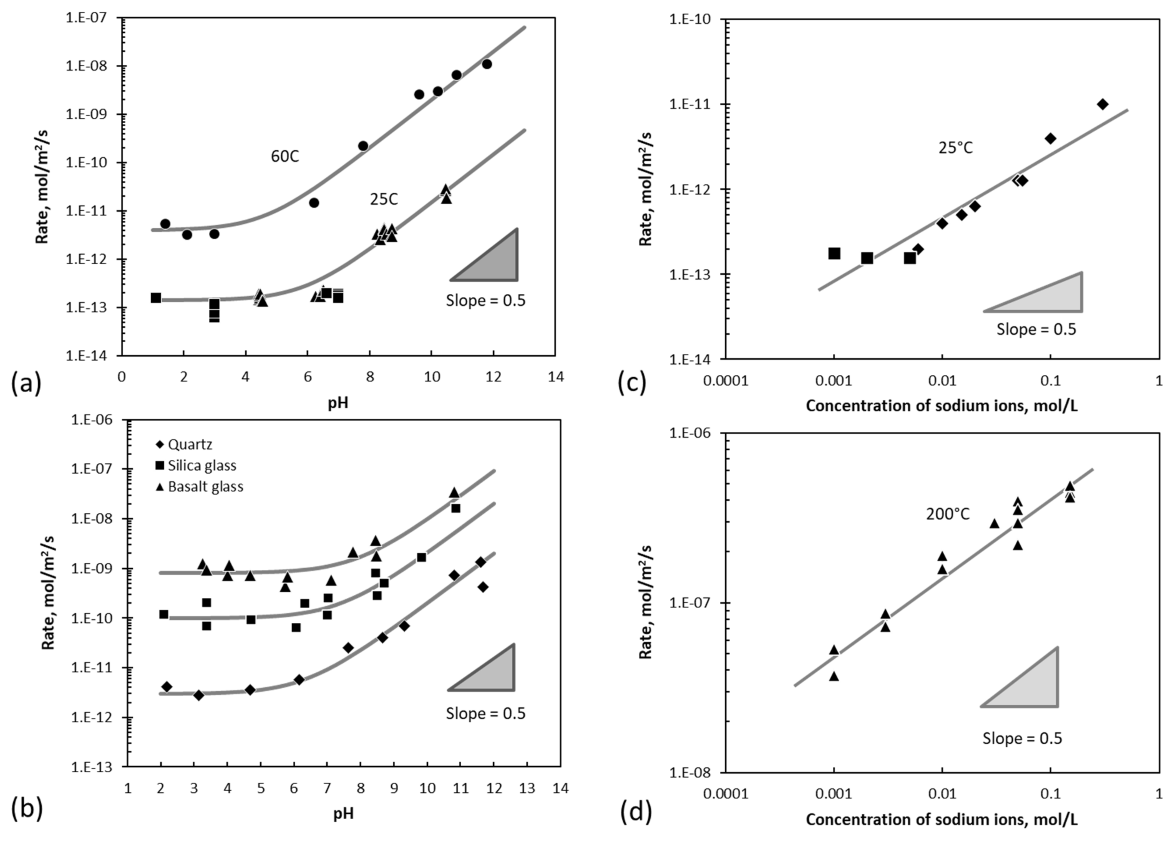
The dissolution of quartz provides an example of more complex kinetic behavior that can be used to test the surface-vacancy model [7]. Data for the dissolution behavior of quartz has been compiled by Bickmore [69], and Rimstidt [70] analyzed this data statistically and showed that the order of reaction with respect to H⁺ is zero in the acid region, while the order of reaction with respect to OH^- is 0.5 in the alkaline region. In addition, it was found that, in the alkaline region, the order of reaction with respect to Na⁺ is 0.5. Some of the data from the Bickmore compilation are shown in Figure 6.

Crundwell [7] proposed that the dissolution of quartz (SiO₂) occurs due to the removal of a ‘cation’ species by Reaction (14) for which the rate expression is Equation (15).

$$\equiv SiO+O{H}^{-}\to SiO{\left(OH\right)}^{+}\left(aq\right)+{\equiv }^{2-}$$

(14)

$$r_{+}={\overrightarrow{k}}_{+}\left[O{H}^{-}\right]exp\left(y\right)$$

(15)

The removal of the ‘anion’ species was proposed to be by the parallel reaction with H⁺ and a Na⁺ catalyzed step, as shown in Reactions (16) and (17).

$$\equiv O+H^{+}\to O{H}^{-}\left(aq\right)+{\equiv }^{2+}$$

(16)

$$\equiv O+H_{2}O\stackrel{N{a}^{+}}{\to }2O{H}^{-}\left(aq\right)+{\equiv }^{2+}$$

(17)

The rate expression for these two parallel reactions is given by Equation (18).

$$r_{-}={\overrightarrow{k}}_{-,1}[H^{+}]exp\left(-y\right)+{\overrightarrow{k}}_{-,2}[N{a}^{+}]exp\left(-y\right)$$

(18)

Equations (15) and (18) are substituted in Equation (9) and solved for the unknown variable $y$, which is a dimensionless form of the potential difference across the surface.

$$\exp \left(2y\right)=\frac{{\overrightarrow{k}}_{-,1}[H^{+}]+{\overrightarrow{k}}_{-,2}[N{a}^{+}]}{{\overrightarrow{k}}_{+}\left[O{H}^{-}\right]}$$

(19)

If Equation (19) is substituted back into Equation (15), the rate of dissolution is given by Equation (20).

$$r_{+}={\left({\overrightarrow{k}}_{+}{\overrightarrow{k}}_{-,1}[H^{+}][O{H}^{-}]+{\overrightarrow{k}}_{+}{\overrightarrow{k}}_{-,2}[N{a}^{+}][O{H}^{-}]\right)}^{1/2}$$

(20)

The term $[H^{+}]\left[O{H}^{-}\right]$ is constant (because it represents the dissociation of water). In the acidic region, the rate is not dependent on pH while in the alkaline region the rate of dissolution is dependent on the pH and the concentration of sodium ions. The lines shown in the graphs in Figure 6 represent the fit of this equation to the data, and a full fit of 285 data points from fourteen different studies shows that this is an excellent description of the data [7].

7. Testing the Surface-Vacancy Model—Thermodynamics

Equilibrium is accounted for by including the kinetics of the reverse reactions for the steps given in Equations (2) and (3). This means that Equations (10) and (11) are expanded as Equations (21) and (22) by including the reverse terms.

$$r_{+}={\overrightarrow{k}}_{+}exp\left(y\right)-{\overleftarrow{k}}_{+}\left[M^{+}\right]exp\left(-y\right)$$

(21)

$$r_{-}={\overrightarrow{k}}_{-}{[H^{+}]}^{t}exp\left(-y\right)-{\overleftarrow{k}}_{-}\left[H_t{A}^{t-1}\right]exp\left(y\right)$$

(22)

Combining these expressions with Equation (9) yields, after some algebraic rearrangement, the rate expression given in Equation (23).

$$rate=\frac{{\overrightarrow{k}}_{+}{\overrightarrow{k}}_{-}{[H^{+}]}^t-{\overleftarrow{k}}_{+}{\overleftarrow{k}}_{-}\left[M^{+}\right]\left[H_t{A}^{t-1}\right]}{{\left({\overrightarrow{k}}_{-}{[H^{+}]}^t+{\overleftarrow{k}}_{+}\left[M^{+}\right]\right)}^{1/2}{\left({\overrightarrow{k}}_{+}+{\overleftarrow{k}}_{-}\left[H_t{A}^{t-1}\right]\right)}^{1/2}}$$

(23)

At equilibrium, the rate is zero. Therefore, the equilibrium condition for this surface-vacancy model can be obtained by setting the left-hand side of Equation (23) to zero. This yields Equation (23). $K$ is clearly the equilibrium constant.

$$\frac{{\overrightarrow{k}}_{+}{\overrightarrow{k}}_{-}}{{\overleftarrow{k}}_{+}{\overleftarrow{k}}_{-}}=\frac{\left[M^{+}\right]\left[H_t{A}^{t-1}\right]}{{[H^{+}]}^t}=K$$

(24)

This clearly demonstrates that the proposed mechanism is consistent with chemical thermodynamics.

8. Testing the Surface-Vacancy Model—Reverse Reaction

8.1. Orders of Reaction for the Reverse Reaction

The reverse reaction, that is, deposition, crystallization and precipitation, can be considered either separately, or in conjunction with Equation (24). Specific orders of reaction have been reported for the reverse reaction for sulfides and for calcite, and the application of the surface-vacancy model to these cases is examined in this section.

Consider the reverse reaction for the dissolution of ZnS given by Equation (25).

$$ZnS+2H^{+}\to Z{n}^{2+}+H_{2}S$$

(25)

Both Locker and de Bruyn [62] and Crundwell and Verbaan [68] reported that the orders of the reverse reaction had values of 0.5 with respect to both Zn²⁺ and H₂S (see Table 4). To describe these results, select a value of 2 for $t$ and consider only terms for the reverse reactions in Equation (16). This yields that the rate of precipitation of ZnS is given by Equation (26).

$$rate of reverse reaction=-{\left( {\overleftarrow{k}}_{+}{\overleftarrow{k}}_{-}\left[Z{n}^{2+}\right]\left[H_{2}S\right]\right)}^{1/2}$$

(26)

This mechanism clearly accounts for the results presented in Table 4 for ZnS and CdS [62].

The dissolution of carbonates presents a similar set of kinetics. Consider the dissolution of calcium carbonate, given by Equation (27).

$$CaC{O}_3\rightleftharpoons C{a}^{2+}+C{O}_3^{-}$$

(27)

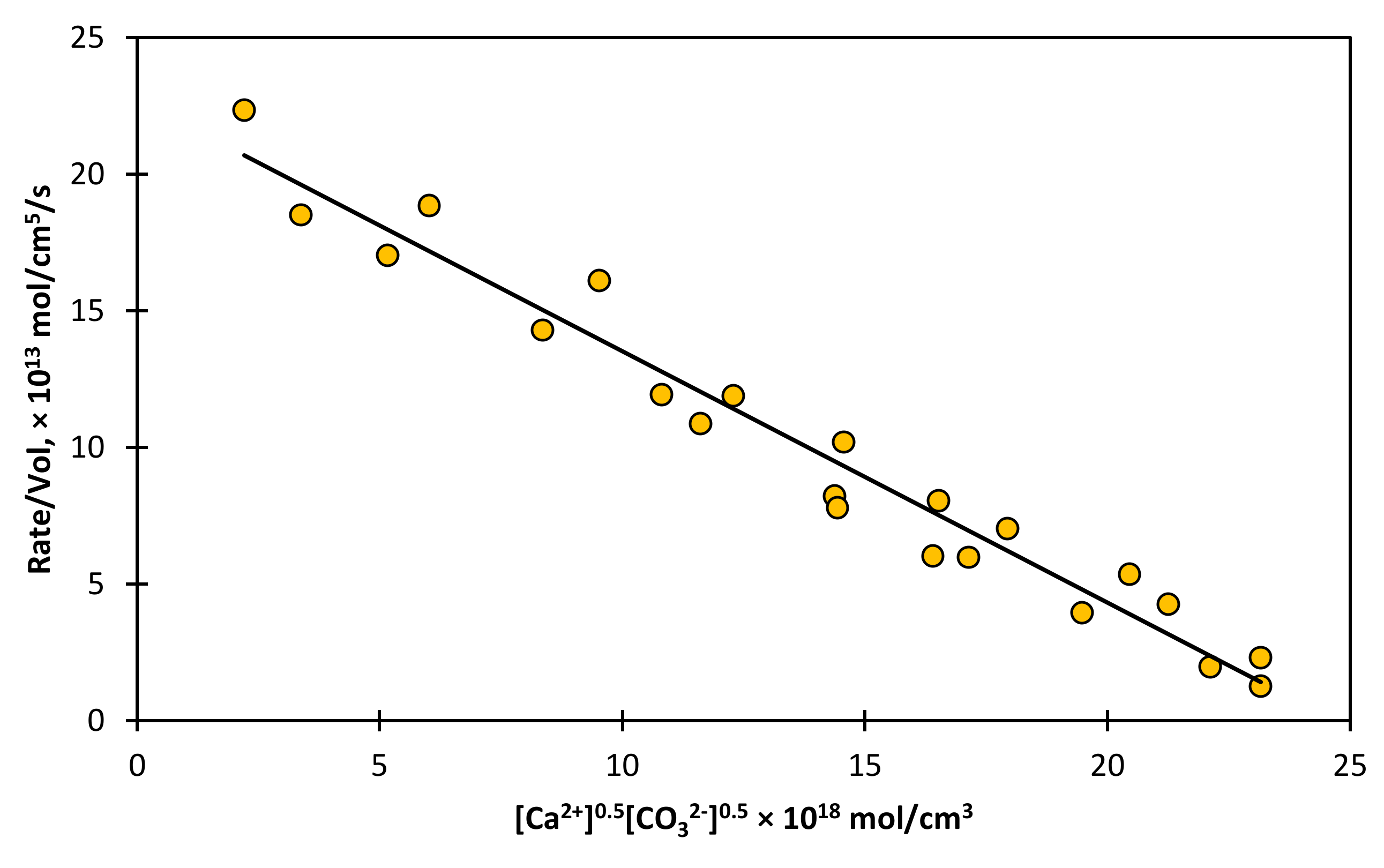
The results of the experiments are shown in Figure 7, which show that the orders of reaction are 0.5 with respect to ${\mathrm{Ca}}^{2+}$ and 0.5 with respect to ${\mathrm{CO}}_3^{2-}$. Bearing in mind the complexities of this reaction, the similarities with ZnS under the conditions used by Sjöberg [71] are quite remarkable.

The rate of the reverse reaction can be obtained directly from Equation (16) by choosing of value of zero for t and considering the cation and anion to be Ca²⁺ and CO₃²⁻. This choice yields Equation (28) for the reverse reaction only. This expression is clearly in agreement with the experimental results shown in Figure 7.

$$rate of reverse reaction=-{\left( {\overleftarrow{k}}_{+}{\overleftarrow{k}}_{-}\left[C{a}^{2+}\right]\left[C{O}_3^{2-}\right]\right)}^{1/2}$$

(28)

The full reaction path between reaction control and equilibrium is discussed next [72].

8.2. Dissolution of Salts between Reaction Control and Equilibrium

The rate expression for the forward reaction for the dissolution of a salt is trivial since the salt only interacts with water, whose concentration is high and nearly always approximately constant. This means that the forward rate is constant with concentration. However, as the concentration of salt in solution increases, the reverse reaction plays a role. As mentioned in the introduction, the reverse reaction is most often accounted for in rate expressions of the form $rate=k{\left(1-\Omega \right)}^m$, where $\Omega$ is equal to activity product divided by the equilibrium constant. The term reaction order has been used for the term $m$ in the rate expression $rate=k{\left(1-\Omega \right)}^m,$ where $\Omega$ is the degree of saturation. This is an empirical rate expression, and the term ‘reaction order’ for $m$ is a misnomer.

For a salt such as NaCl, $\Omega$ is given by $\left[N{a}^{+}\right]\left[C{l}^{-}\right]/K$. If the rate is expressed in terms of the concentration of salt, $C$, then this form of the rate expression is given by $rate=k\left(1-C^2\right)$, where $C=\left[NaCl\right]=\left[N{a}^{+}\right]=\left[C{l}^{-}\right]={[N{a}^{+}]}^{1/2}{\left[C{l}^{-}\right]}^{1/2}$, and the value of $m$ is taken as 1 for the sake of simplicity. Thus, this expression means that the rate decreases as a parabolic function of increasing salt concentration, $C$, representing the path from rate control to equilibrium [8,72].

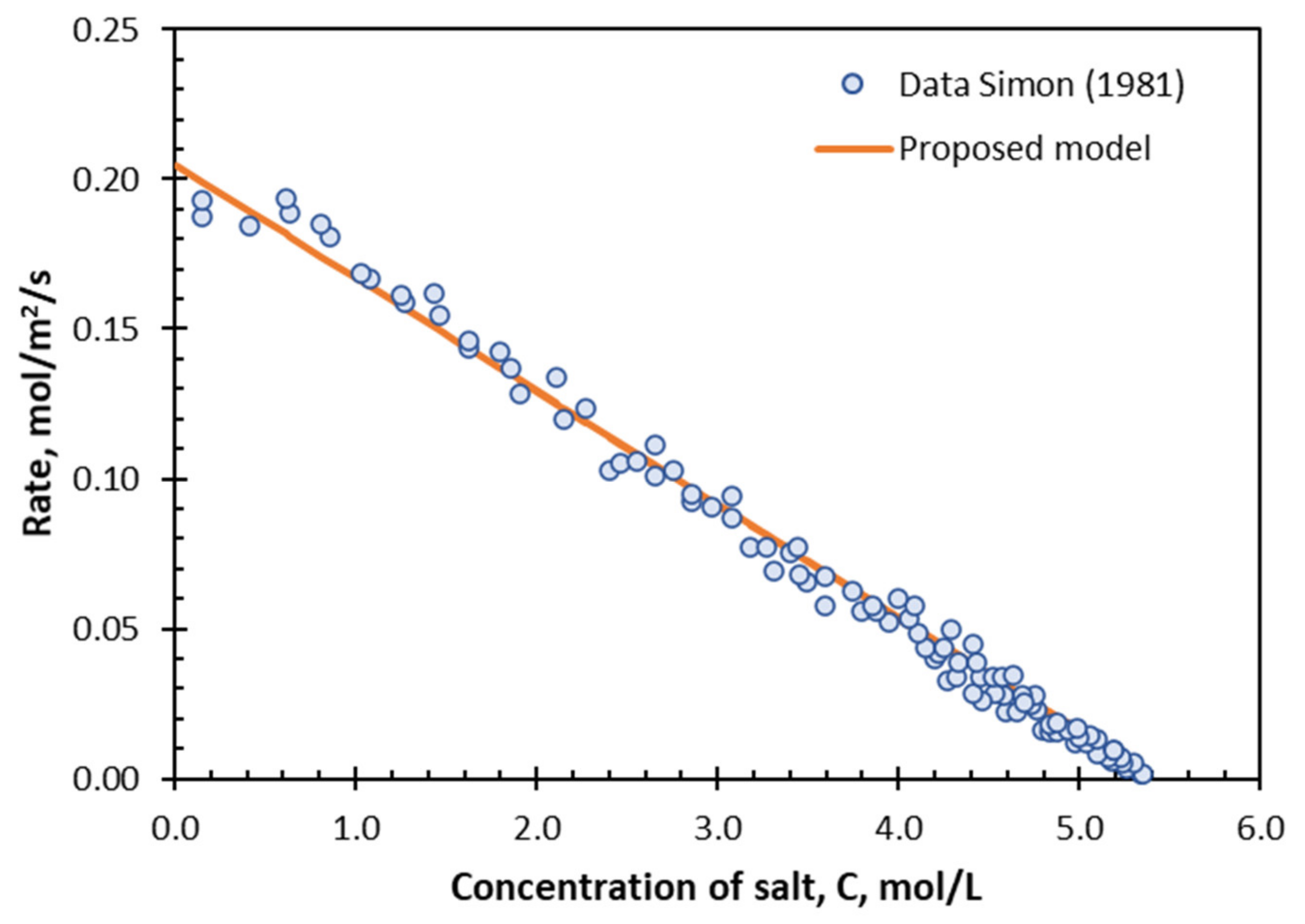
The rate of dissolution of NaCl is shown in Figure 8 as a function of the concentration of NaCl in solution, $C$. This is not a parabolic function—in contrast, it is linear.

The linear relationship between the rate of dissolution and the concentration of NaCl means that the rate expression is $rate=k_f-k_r{[N{a}^{+}]}^{1/2}{\left[C{l}^{-}\right]}^{1/2}$. The similarities with the results for ZnS, CdS, and CaCO₃ in the previous sections are difficult to miss.

The full rate expression is derived from Equation (23) by choosing the value of zero for t and using the Equation (24) for the equilibrium concentration. This yields Equation (29)

$$rate=\frac{{\overrightarrow{k}}_{+}{\overrightarrow{k}}_{-}-{\overleftarrow{k}}_{+}{\overleftarrow{k}}_{-}\left[N{a}^{+}\right]\left[C{l}^{-}\right]}{{\left({\overrightarrow{k}}_{-}+{\overleftarrow{k}}_{+}\left[N{a}^{+}\right]\right)}^{1/2}{\left({\overrightarrow{k}}_{+}+{\overleftarrow{k}}_{-}\left[C{l}^{-}\right]\right)}^{1/2}}=\frac{k_1\left(1-\left[N{a}^{+}\right]\left[C{l}^{-}\right]/K\right)}{{\left(k_2+\left[N{a}^{+}\right]\right)}^{1/2}{\left(K/k_{2+}+\left[C{l}^{-}\right]\right)}^{1/2}}$$

(29)

The rate constant ${\mathrm{k}}_1$ is given by ${\overrightarrow{k}}_{+}{\overrightarrow{k}}_{-}/{\left({\overleftarrow{k}}_{+}{\overleftarrow{k}}_{-}\right)}^{1/2}$ and ${\mathrm{k}}_2$ is given by ${\overrightarrow{k}}_{-}/{\overleftarrow{k}}_{+}$. The line in Figure 8 represents the best fit of Equation (29) to the data.

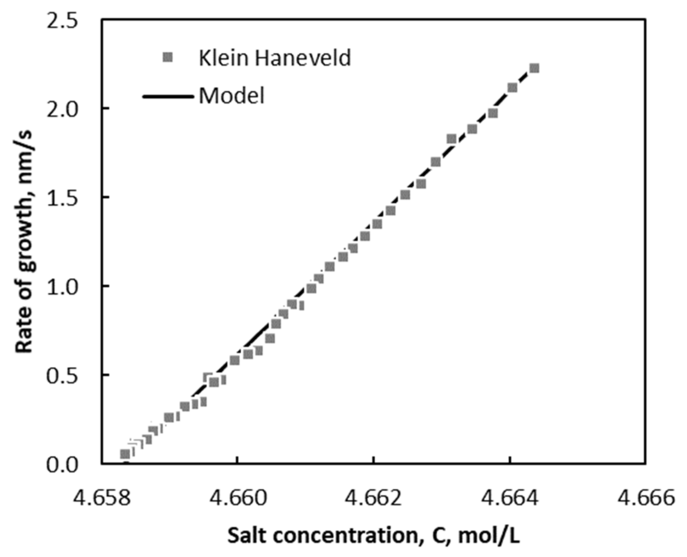
This linear dependence on C, and hence half-order kinetics, is echoed in crystallization studies. Figure 9 shows the growth of KCl as a function of the concentration of salt, C, divided by the saturated concentration of salt, $C$. The line in Figure 9 represents the fit of Equation (29) to this data set.

8.3. Rate Formulation Based on Chemical Affinity

The approach to equilibrium is sometimes modelled in dissolution studies using the chemical affinity [75]. For a solid MA, the chemical affinity, $A$, is defined by Equation (30).

$$A=-RTln\left(\left[M^{+}\right]\left[A^{-}\right]/K\right)$$

(30)

In some cases, the plot of $rate$ against $A$ gives an S-shape, which is difficult to explain with a simple reverse reaction. An example of such an S-shape is shown in Figure 10 for the feldspar albite.

The surface-vacancy model describes this observation. The substitution of Equation (30) into Equation (23) yields Equation (31) for the generic solid MA.

$$rate=\frac{k_1\left(1-exp\left(-A/RT\right)\right)}{{\left(k_2+\left[M^{+}\right]\right)}^{1/2}{\left(K/k_{2+}+\left[A^{-}\right]\right)}^{1/2}}$$

(31)

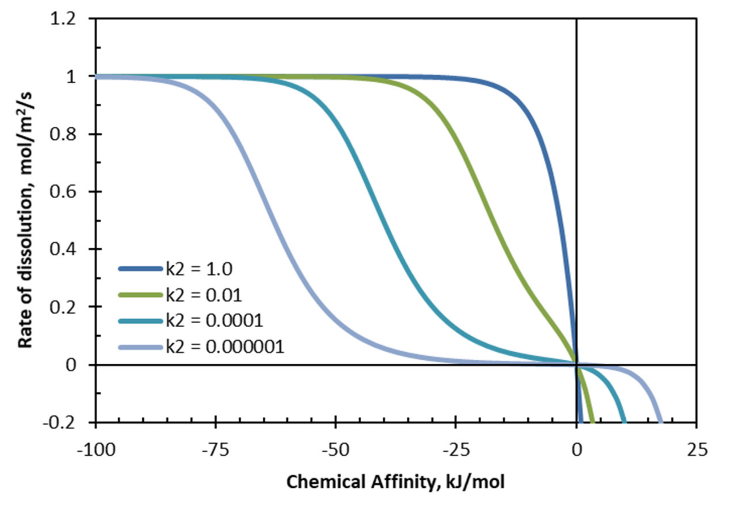
The rate for the surface-vacancy model as a function of chemical affinity is plotted in Figure 11 for different values of $k_2$. The chemical affinity in Figure 11 was varied by simultaneously changing the value of the concentrations of $M^{+}$ and $A^{-}$ so that $\left[{\mathrm{M}}^{+}\right]$ is equal to $\left[{\mathrm{A}}^{-}\right]$ at each position on the curve. Clearly, the surface-vacancy model can account for the change from monotonic form to the S-shape found for some minerals such as albite.

The line in Figure 10 represents a fit of the surface-vacancy model to the data for albite, showing that the surface-vacancy model is a good description of this reaction under these conditions.

8.4. Rate Formulation Based on Degree of Saturation

The rate of dissolution over the range between reaction control and equilibrium has also been analyzed in terms of the degree of saturation, $\Omega$, which is equal to the activity product divided by the equilibrium constant. Equation (31) can be written in this form as Equation (32).

$$rate=\frac{k_1\left(1-\Omega \right)}{{\left(k_2+\left[M^{+}\right]\right)}^{1/2}{\left(K/k_{2+}+\left[A^{-}\right]\right)}^{1/2}}$$

(32)

The rate is plotted as a function of $1-\Omega$ in Figure 12 assuming that $\Omega$ is varied by simultaneously changing the value of the concentrations of $M^{+}$ and $A^{-}$ so that $\left[{\mathrm{M}}^{+}\right]$ is equal to $\left[A^{-}\right]$ at each point (yielding the special case that $\left[M^{+}\right]=\left[A^{-}\right]={\left(\Omega \right)}^{1/2}$).

Note the deviation from linearity in Figure 12a as $\Omega$ tends towards 0 that is, the right-hand side of Figure 12a,b as $1-\Omega$ tends to 1. This non-linearity is due to the contribution of the denominator in Equation (32), which is only predicted by the surface vacancy model.

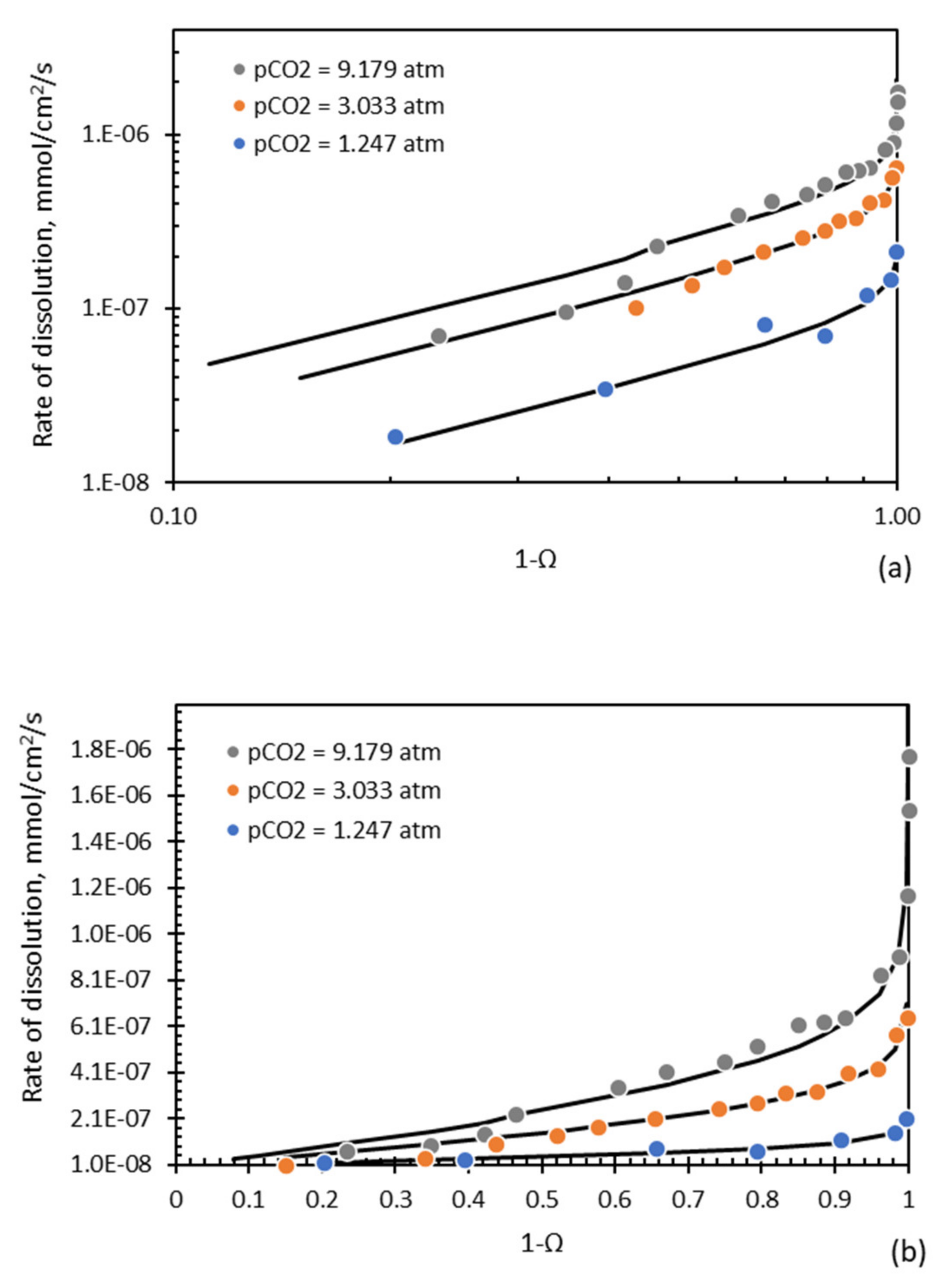
There is evidence to support this non-linearity. Consider the results reported by Busenberg and Plummer [77] for the dissolution of calcite shown in Figure 13 as a function of $1-\Omega$. These results clearly display the non-linearity of the curve as $1-\Omega$ approaches 1. As the partial pressure of CO₂ was maintained in these tests, the results are modelled by Equation (33), where ${\mathrm{k}}_3$ accounts for the anion terms for either carbonate or bicarbonate or both. Busenberg and Plummer [77] reported values for both $\Omega$ and $\left[{\mathrm{Ca}}^{+}\right]$.

$$rate=\frac{k_1\left(1-\Omega \right)}{{\left(k_2+\left[C{a}^{+}\right]\right)}^{1/2}{k}_3}$$

(33)

This simplified model clearly accounts for the results of Busenberg and Plummer [76], especially the non-linearity as $1-\Omega$ approaches 1.

For the results of Sjoberg [71] and these results to both hold true, it would mean that Sjoberg’s investigations were carried out in this non-linear region. Obviously, there are more details of this reaction than have been presented here and further investigation is required; however, these examples demonstrate the promise of the surface-vacancy model that might allow different aspects of the puzzle of calcite dissolution to be reconciled.

9. Testing the Surface-Vacancy Model—Initial Rates of Dissolution

When a solid is added to an aqueous solution in which it can dissolve, the rate of dissolution is initially fast and then slows. This is frequently interpreted as ‘passivation’, or a limitation posed by a surface layer—but this is not always the case.

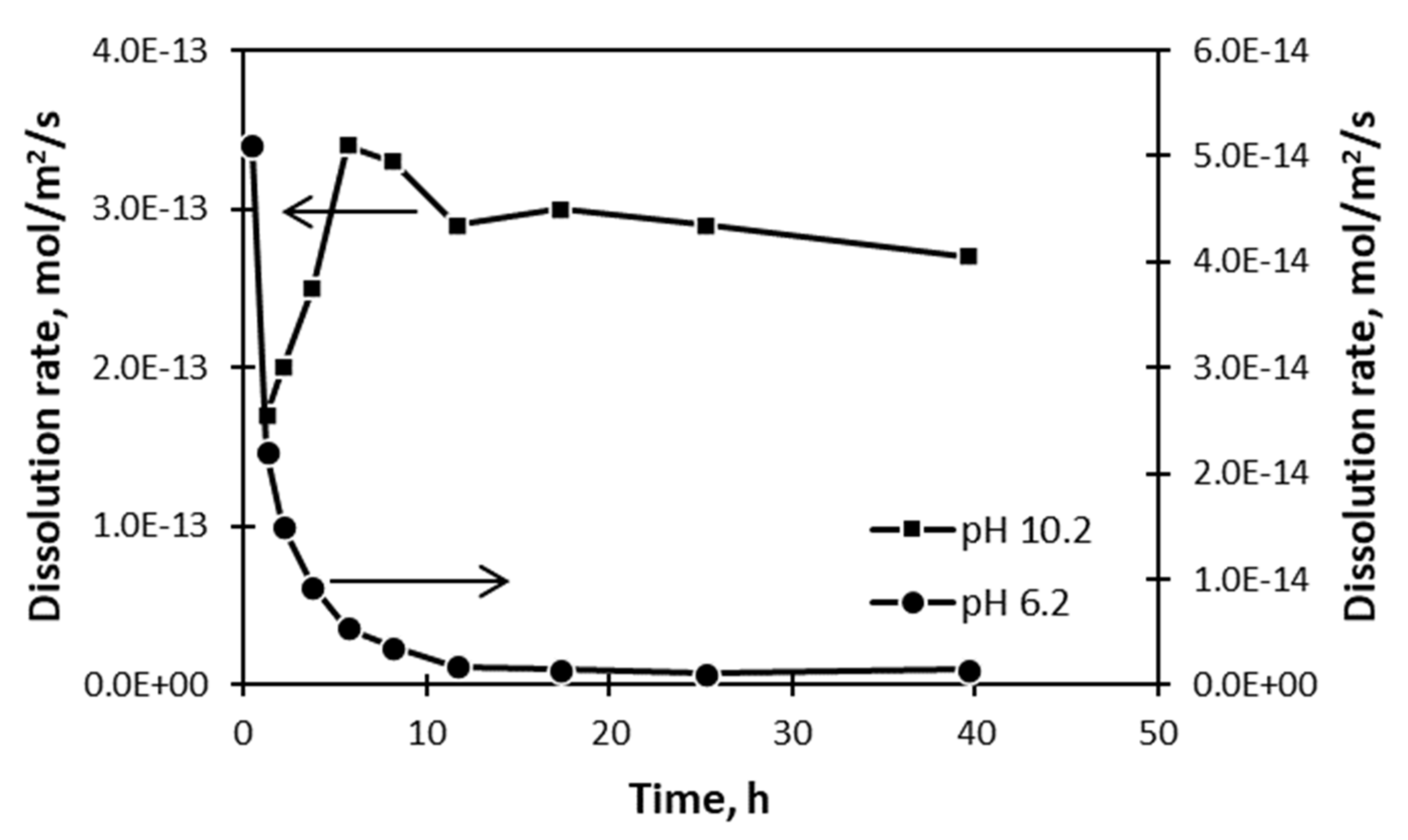
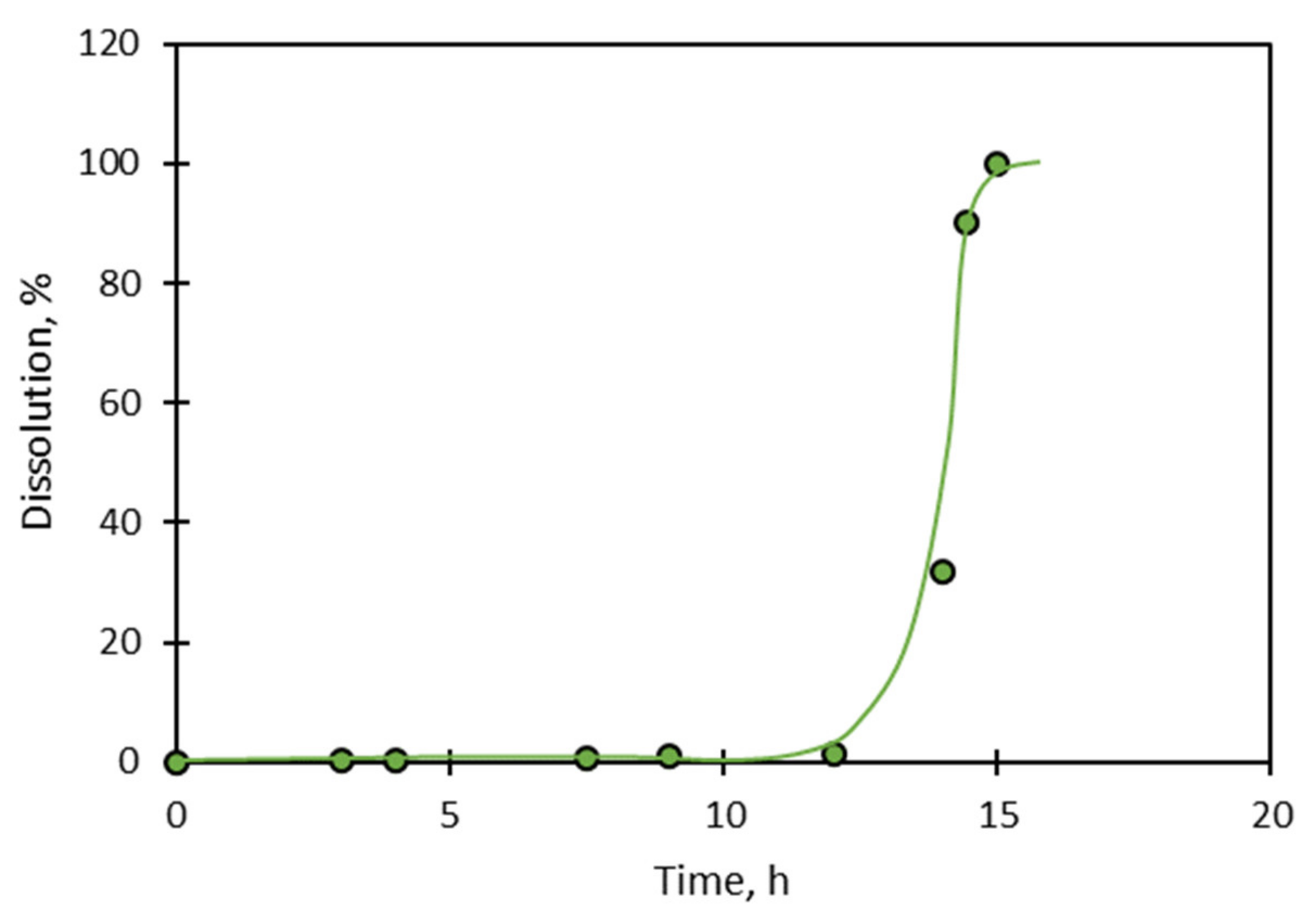
Consider the dissolution of quartz at pH 6.2, as shown in Figure 14. Even though the rate of dissolution is initially fast and then slows, it reaches a steady state rate at which it continues to dissolve. That the solid continues to dissolve creates difficulties for the surface layer proposal, which means that it must be modified that limit growth of the layer once a certain thickness has been attained. No conditions have been set or derived by these layer models that determine such thickness, or how steady-state dissolution continues in its presence.

These difficulties with models based on surface layers are compounded when it is considered that the rate of dissolution of these same solids might initially accelerate in different circumstances. Figure 14 also shows that the rate of dissolution of quartz at pH 10.2 is initially slow, and then accelerates to a steady or stationary value. Layer formation cannot explain such an accelerating rate of dissolution.

Similar results have been reported for NiO and AgBr. The acceleration of the dissolution of NiO is shown in Figure 15.

The surface vacancy model accounts for this phenomenon without any additional physical modifications. In order to progress from Equation (8) to Equation (9), stationary conditions were assumed. To account for non-stationary effects, Equation (8) should be used instead of Equation (9).

The surface charge, ${\mathsf{\sigma }}_0$, is a proportional to the potential difference across the Helmholtz layer, with the proportionality constant referred to as the electrical capacitance of the layer. This means that Equation (8) can be written as Equation (34).

$$\frac{d\Delta \varphi }{dt}=\frac{F}{C_d}\left({\nu }_{-}{r}_{-}-{\nu }_{+}{r}_{+}\right)$$

(34)

If the reaction is far from equilibrium, $r_{+}$ and $r_{-}$ are given by Equations (10) and (11). Substituting these values into Equation (34) and taking note that $y$ is a dimensionless form of the potential difference, the expression is written in terms of $y$.

$$\frac{2RT{C}_d}{F^2}\frac{dy}{dt}={\nu }_{-}{\overrightarrow{k}}_{-}{[H^{+}]}^{t}exp\left(-y\right)-{\nu }_{+}{\overrightarrow{k}}_{+}exp\left(y\right)$$

(35)

This equation needs to be combined with the batch mass balances for the concentrations of ions in solution. These mass balances are given by Equations (36) and (37).

$$\frac{dV\left[M^{+}\right]}{dt}=r_{+}V$$

(36)

$$\frac{dV\left[A^{-}\right]}{dt}=r_{-}V$$

(37)

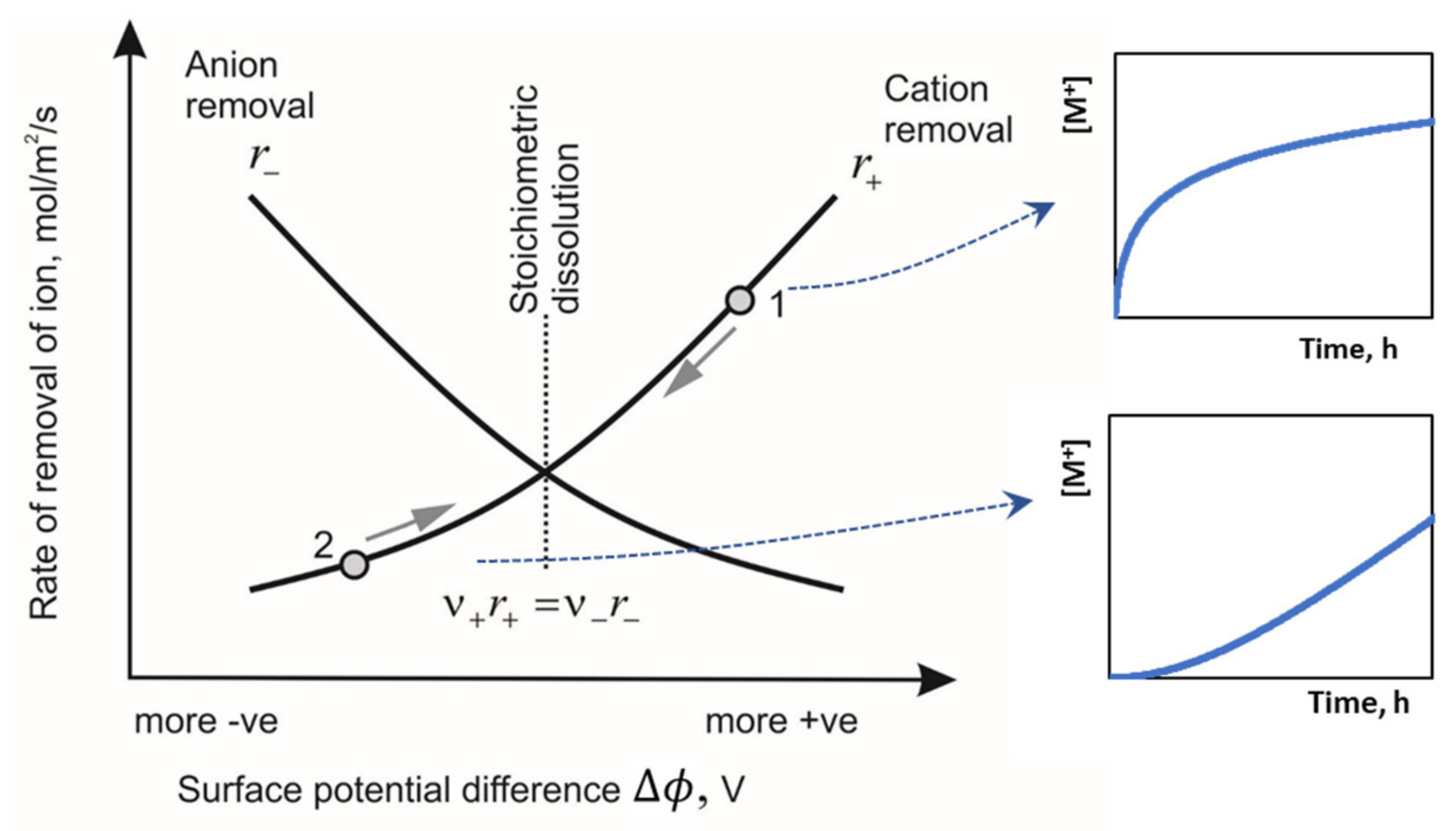
The curves for the rate of dissolution of the cation and the anion, given by Equations (10) and (11), are shown in Figure 16 as a function of potential difference across the Helmholtz layer, noting that $y$ is a dimensionless form of potential difference. The point at which stationary dissolution occurs is where Equation (9) is applicable and is at the intersection of the two curves. Most of the analysis on the orders of reaction and equilibrium has assumed that the experiments in question have been conducted at this stationary point.

The rate of dissolution is typically tracked by measuring only one of the constituent ions. Consider the case in which the cation is measured as it accumulates in solution. If the solid has an initial surface charge on immersion that is more positive than point of stationary dissolution, illustrated as point 1 in Figure 16, then the positive charge will favor the removal of cations. The rate at potential 1 for cations is higher than that for anions, and as more cations are removed the surface becomes more negative, in turn lowering the potential and surface charge. This means that there is a driving force towards the stationary point. Turning attention to the rate of dissolution of cations, we see that it is initially highest, and then decreases until it reaches the stationary point where stoichiometric dissolution takes place.

If, on the other hand, the potential is initially more negative than the stationary point, then the removal of anions is more favorable, which makes the surface more positive, and this creates a driving force towards the stationary point. The dissolution of cations, though, is initially slow, and accelerates as the potential moves to the stationary point.

Thus, the surface-vacancy model describes both the acceleration and deceleration of the initial rates of dissolution.

10. Testing the Surface-Vacancy Model—Non-Stoichiometric Dissolution

Non-stoichiometric dissolution occurs by the same mechanism as discussed in the previous section, except that both anion and cation are measured, and the fact that the rates of dissolution are different is exposed. There is always a non-stoichiometric period initially before the surface charge has reached a stationary state. Stoichiometric is guaranteed only at the stationary point described by Equation (9), which incidentally is a stable operating point. Of course, for solids that dissolve quickly, the non-stoichiometric period might be very short.

11. Independent Testing of the Surface—Vacancy Model

The surface-vacancy model proposed here is based on a clearly described physical model of the surface. It posits that the surface is charged because the removal of ions leaves vacancies of opposite charge to the ions themselves. Thus, the predictions of the surface-vacancy model can be tested by measurements of the surface charge.

The surface-vacancy model has been applied to the data for the zeta potential of several minerals that are of importance to flotation has been examined [79]. In that work, it was shown that the surface-vacancy model successfully described the measurements of the zeta potential. In other work, the surface-vacancy model has been shown to describe the measurements of zeta potential in a manner that is consistent with the mechanism of dissolution of quartz and silica [7] and forsterite [9].

The most common explanation for the surface charge is the multisite complexation model of Hiemstra et al. [80,81]. This model is a combination of the ‘amphoteric model’ and the ‘one-pK model’, both of which suffer from unclear and possibly indefensible foundations. For example, the multi-site complexation model assigns arbitrary values to the charge of a surface ion. Thus, it is proposed that the surface vacancy model is not only a model of dissolution but could be a foundational model for surface charge.

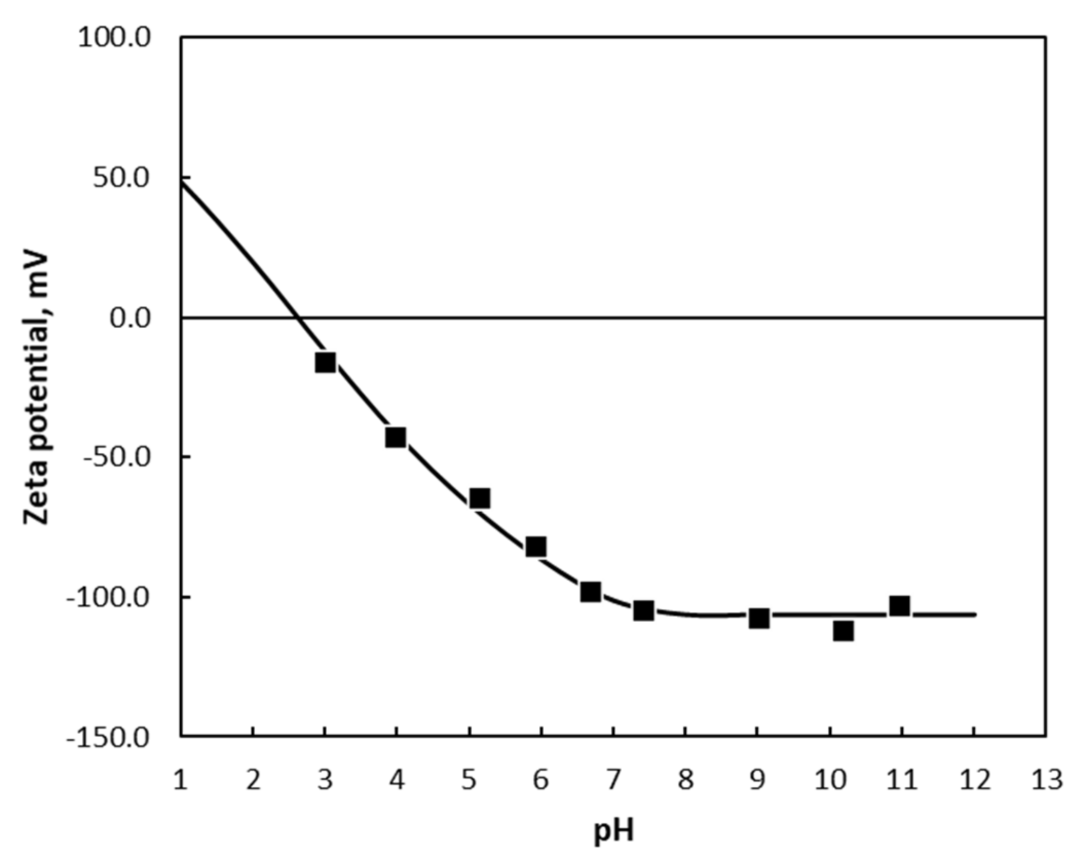
Surface charge, through independent measurements such as zeta potential, can be used as a clear and independent verification of the proposed model. As an example of this, consider the zeta potential of quartz, shown in Figure 17.

The potential difference across the interface for quartz during dissolution is given by Equation (19). Examination of this equation reveals that the potential difference is proportional to the pH in the acid region. As the concentration of Na⁺ is close to the concentration of OH⁻ in the alkaline region, it is independent of the pH in the alkaline region. This is precisely what is given by the data of James and Healy [82] shown in Figure 17. This demonstrates that the mechanism proposed for dissolution is effective in describing the surface charge.

12. Predictions from the Surface—Vacancy Model

The surface-vacancy model envisages the chemically independent removal of cations and anions, with the relationship between them governed only by surface charge (or the potential difference across the Helmholtz layer). Equilibrium, therefore, can be achieved in a partial manner [4,72]. A set of conditions can be envisaged in which one of the ‘partial reactions’ is in equilibrium, while the other is not. This situation is referred to as partial equilibrium, and it is possible that laboratory experiments in which it was assumed that the conditions were at equilibrium are in fact only at ‘partial equilibrium’. This is a unique view of equilibrium conditions and may have far reaching implications for the interpretation of experimental work in this field.

The surface vacancy model can account for the effect of other ligands. This has been treated in mechanisms for forsterite dissolution [9].

The model can also account for the effect of impurities in solution on the rate of dissolution by including their deposition onto and their removal from the surface. This is an area for future work.

13. Oxidative and Reductive Dissolution

The discussion in this paper has focused on the dissolution of minerals in which no oxidation or reduction in the mineral takes place. Specifically, this is referred to as non-oxidative dissolution. Oxidation and reductive dissolution reactions are those in which oxidation or reduction in the mineral occurs during dissolution. Oxidative and reductive dissolution reactions are industrially important because the rates of these reactions are generally faster than the non-oxidation dissolution for the corresponding mineral.

Consequently, there has been extensive examination of the mechanism of oxidative dissolution in the metallurgical literature [83,84,85,86]. The influence of oxidants and reductants in solution is well documented. Research on the influence of the electronic structure of the mineral is beginning to make progress [84,85,86], while advanced models for the effect of the content of iron in sphalerite, (Zn,Fe)S, on both the rate and activation energy of dissolution have been developed [84,86].

There are aspects of oxidative and reductive dissolution reaction that share features with the non-oxidative reactions analyzed in this paper. Most obvious is that oxidative and reductive dissolution frequently exhibit half-order kinetics with respect to oxidant or reductant. This half-order is described by the mixed-potential model [87]. Many of the features of non-oxidative dissolution highlighted here might be applicable to oxidative dissolution reactions. Despite possible similarities between the mixed-potential model and the surface-vacancy model, there are major differences in their physical foundations. In oxidative and reductive dissolution, the surface charge is envisaged to be caused by excess electrons, whereas in the surface-vacancy model, the surface charge is envisaged to be caused by ionic vacancies on the surface.

This difference in nature of charge formation might seem immaterial. On the contrary, it is profound—it is not possible to understand the formation of surface charge during non-oxidative dissolution without the surface-vacancy model. Indeed, the surface-vacancy model is primarily a model of surface charge, with dissolution both the cause and the consequence.

14. Conclusions

This paper has demonstrated that there is a need for a new model of dissolution and has reviewed the novel proposal of the surface-vacancy model. The attention of this paper has focused on the physical foundations of this model, which provide clear independent tests of the model. Specifically, it has been shown (i) that the surface-vacancy model is applicable to the non-oxidative dissolution of all minerals and salts, (ii) that it provides a clear physical foundation from which the rate equations are derived, (iii) the rate expressions derived from this physical model describe the effects of H⁺ and OH^- on the rate of dissolution expressed in terms of the order of reaction with respect to these reactants, (iv) that it describes the approach to equilibrium, (iv) that it describes the change in rate of dissolution during the initial stage of reaction and (v) that it describes the non-stoichiometric dissolution of more complex solids.

Most importantly, this model inherently and coherently describes the formation surface charge and the effect of this charge on the rate of removal and deposition of ions and demonstrates how this leads to orders of reaction that are multiples of one-half.

It has been demonstrated that the physical foundations of the model are testable by independent means, principally by measurements of the surface charge or surface potential difference. Finally, the model predicts a state of ‘partial equilibrium’ that is not contemplated other models.

Further work should be focused on assessing the foundations of the model, that is, the mechanism of surface charging due to surface vacancies, and the application of this novel physical foundation to other fields, such as crystallization, flotation, and colloid science.

References

- Crundwell, F.K. The mechanism of dissolution of minerals in acidic and alkaline solutions: Part I—A new theory of non-oxidation dissolution. Hydrometallurgy 2014, 149, 252–264. [Google Scholar] [CrossRef]
- Crundwell, F.K. The mechanism of dissolution of minerals in acidic and alkaline solutions: Part II Application of a new theory to silicates, aluminosilicates and quartz. Hydrometallurgy 2014, 149, 265–275. [Google Scholar] [CrossRef]
- Crundwell, F.K. The mechanism of dissolution of minerals in acidic and alkaline solutions: Part III. Application to oxide, hydroxide and sulfide minerals. Hydrometallurgy 2014, 149, 71–81. [Google Scholar] [CrossRef]
- Crundwell, F.K. The mechanism of dissolution of minerals in acidic and alkaline solutions: Part IV—Equilibrium and near equilibrium behaviour. Hydrometallurgy 2015, 153, 46–57. [Google Scholar] [CrossRef]
- Crundwell, F.K. The mechanism of dissolution of minerals in acidic and alkaline solutions: Part V—Surface charge and zeta potential. Hydrometallurgy 2016, 162, 174–184. [Google Scholar] [CrossRef]
- Crundwell, F.K. The mechanism of dissolution of minerals in acidic and alkaline solutions: Part V—A molecular viewpoint. Hydrometallurgy 2016, 161, 34–44. [Google Scholar] [CrossRef]
- Crundwell, F.K. On the mechanism of the dissolution of quartz and silica in aqueous solutions. ACS Omega 2017, 2, 1116–1127. [Google Scholar] [CrossRef] [PubMed]
- Crundwell, F.K. The impact of surface charge on the ionic dissociation of common salt (NaCl). Chem. Eng. Sci. 2019, 205, 174–180. [Google Scholar] [CrossRef]
- Crundwell, F.K. The mechanism of dissolution of forsterite, olivine and minerals of the orthosilicate group. Hydrometallurgy 2014, 150, 68–82. [Google Scholar] [CrossRef]
- Crundwell, F.K. The mechanism of dissolution of the feldspars: Part I. Dissolution at conditions far from equilibrium. Hydrometallurgy 2015, 151, 151–162. [Google Scholar] [CrossRef]
- Crundwell, F.K. The mechanism of dissolution of the feldspars: Part II dissolution at conditions close to equilibrium. Hydrometallurgy 2015, 151, 163–171. [Google Scholar] [CrossRef]
- Knauss, K.G.; Worley, W.G. The dissolution kinetics of quartz as a function of pH and time at 70 °C. Geochim. Cosmochim. Acta 1988, 52, 43–53. [Google Scholar] [CrossRef]
- Crundwell, F.K. Concerning the influence of surface charge on the rate of growth of surfaces during crystallization. Cryst. Growth Des. 2016, 16, 5877–5886. [Google Scholar] [CrossRef]
- Roman, R.J.; Fuerstenau, M.C.; Seidel, D.C. Mechanisms of soluble salt flotation. Part I. Trans. AIME 1968, 241, 56–64. [Google Scholar]
- Rastogi, R.P.; Shukla, R.D. Precipitation and dissolution potentials. J. Appl. Phys. 1970, 41, 2787–2795. [Google Scholar] [CrossRef]
- Ibl, N.; Richardz, W.; Wiederkehr, H. The connection between electric potential and crystallization. Zeitschrift Physikasche Chem. N. F. 1975, 98, 123–142. [Google Scholar] [CrossRef]
- Miller, J.D.; Yalamanchili, M.R.; Kellar, J.J. Surface charge of alkali halide particles as determined by laser-Doppler electrophoresis. Langmuir 1992, 8, 1464–1469. [Google Scholar] [CrossRef]
- Lanaro, G.; Patey, G.N. Molecular Dynamics simulation of NaCl dissolution. J. Phys. Chem. B 2015, 119, 4275–4283. [Google Scholar] [CrossRef]
- Lüttge, A.; Arvidson, R.S.; Fischer, C. A stochastic treatment of dissolution kinetics. Elements 2013, 9, 183–188. [Google Scholar] [CrossRef]
- Ohtaki, H.; Fukushima, N.; Okada, I. Dissolution process of sodium chloride crystal in water. Pure Appl. Chem. 1988, 60, 1321–1324. [Google Scholar] [CrossRef]
- Henriksen, N.E.; Hansen, F.Y. Theories of Molecular Reaction Dynamics—The Foundations of Chemical Kinetics, 2nd ed.; Oxford University Press: Oxford, UK, 2019. [Google Scholar]
- Blum, A.; Lasaga, A. Role of surface speciation in the low temperature dissolution of minerals. Nature 1988, 331, 431–433. [Google Scholar] [CrossRef]
- Furrer, G.; Stumm, W. The coordination chemistry of weathering: I. Dissolution kinetics of δ-Al2O3 and BeO. Geochim. Cosmochim. Acta 1988, 50, 1847–1860. [Google Scholar] [CrossRef]
- Zinder, B.; Furrer, G.; Stumm, W. The coordination chemistry of weathering: II. Dissolution of Fe (III) oxides. Geochim. Cosmochim. Acta 1988, 50, 1861–1869. [Google Scholar] [CrossRef]
- Casey, W.H.; Ludwig, C. The mechanism of dissolution of oxide minerals. Nature 1996, 381, 506–509. [Google Scholar] [CrossRef]
- Pokrovsky, O.S.; Schott, J. Forsterite surface composition in aqueous solutions: A combined potentiometric, electrokinetic, and spectroscopic approach. Geochim. Cosmochim. Acta 2000, 64, 3299–3312. [Google Scholar] [CrossRef]
- Pokrovsky, O.S.; Schott, J. Kinetics and mechanisms of forsterite dissolution at 25 °C and pH from 1 to 12. Geochim. Cosmochim. Acta 2000, 64, 3313–3325. [Google Scholar] [CrossRef]
- Oelkers, E.H. An experimental study of forsterite dissolution rates as a function of temperature and aqueous Mg and Si concentrations. Chem. Geol. 2001, 175, 485–494. [Google Scholar] [CrossRef]
- Oelkers, E.H. General kinetic description of multioxide silicate mineral and glass dissolution. Geochim. Cosmochim. Acta 2001, 65, 3703–3719. [Google Scholar] [CrossRef]
- Dove, P.M.; Han, N.; De Yoreo, J.J. Mechanisms of classical crystal growth theory explain quartz and silicate dissolution behaviour. Proc. Natl. Acad. Sci. USA 2005, 102, 15357–15362. [Google Scholar] [CrossRef] [Green Version]
- Lyklema, J. Electrified interfaces in aqueous dispersions of solids. Pure Appl. Chem. 1991, 63, 895–906. [Google Scholar] [CrossRef]
- Bockris, J.O.M.; Reddy, A.K.N. Modern Electrochemistry; Plenum Press: New York, NY, USA, 1970; Volume 2. [Google Scholar]
- Chen, Y.; Brantley, S.L. Dissolution of forsteritic olivine at 65C and 2 < pH < 5. Chem. Geol. 2000, 165, 267–281. [Google Scholar] [CrossRef]
- Grandstaff, D.E. The Dissolution Rate of Forsteritic Olivine from Hawaiian Beach Sand. In Rates of Chemical Weathering of Rocks and, Minerals; Colman, S.M., Dethier, D.P., Eds.; Academic Press: Orlando, FL, USA, 1986; pp. 41–59. [Google Scholar]
- Haenchen, M.; Prigiobbe, V.; Storti, G.; Seward, T.M.; Mazzotti, M. Dissolution kinetics of forsteritic olivine at 90–150 °C including effects of the presence of CO2. Geochim. Cosmochim. Acta 2006, 70, 4403–4416. [Google Scholar] [CrossRef]
- Olsen, A.A.; Rimstidt, J.D. Oxalate promoted forsterite dissolution at low pH. Geochim. Cosmochim. Acta 2008, 72, 1758–1766. [Google Scholar] [CrossRef]
- Rosso, J.J.; Rimstidt, J.D. A high-resolution study of forsterite dissolution rates. Geochim. Cosmochimica Acta 2000, 64, 797–811. [Google Scholar] [CrossRef]
- Wogelius, R.A.; Walther, J.V. Forsterite dissolution kinetics at near-surface conditions. Chem. Geol. 1992, 97, 101–112. [Google Scholar] [CrossRef]
- Pulfer, K.; Schindler, P.W.; Westall, J.C.; Grauer, R. Kinetics and mechanisms of dissolution of bayerite (γ-Al2O3) in HNO3-HF solutions at 298.2 K. J. Colloid Interface Sci. 1984, 101, 554–564. [Google Scholar] [CrossRef]
- Koch, G. Kinetik und mechanismus der auflösung von berylliumoxyd in säuren. Ber. Der Bunsenges. Phys. Chem. 1965, 69, 141–145. [Google Scholar] [CrossRef]
- Vermilyea, D.A. The dissolution of ionic compounds in aqueous media. J. Electrochem. Soc. 1966, 113, 1067–1070. [Google Scholar]
- Arnison, B.J.; Segall, R.L.; Smart, R.C.; Turner, P.S. Semiconducting oxides: The effects of solid and solution properties on dissolution kinetics of cobaltous oxide. J. Chem. Soc. Faraday Trans. 1978, 77, 535–545. [Google Scholar] [CrossRef]
- Gorichev, I.G.; Kipriyanov, N.A. Regular kinetic features of the dissolution of metal oxides in acidic media. Russ. Chem. Rev. 1984, 53, 1039–1061. [Google Scholar] [CrossRef]
- Seo, M.; Furuichi, R.; Okamoto, G.; Sato, N. Dissolution of hydrous chromium oxide in acid solutions. Trans. Jap. Inst. Met. 1975, 16, 519. [Google Scholar] [CrossRef] [Green Version]
- Majima, H.; Awakura, Y.; Yakazi, T.; Chikamori, Y. Acid dissolution of cupric oxide. Metall. Trans. B 12B 1980, 209–214. [Google Scholar] [CrossRef]
- Furuichi, R.; Sato, N.; Okamoto, G. Kinetics of Fe (OH)3 dissolution. Chimia 1969, 23, 455. [Google Scholar]
- Vermilyea, D.A. The dissolution of MgO and Mg (OH)2 in aqueous solutions. J. Electrochem. Soc. 1969, 116, 1179–1183. [Google Scholar] [CrossRef]
- Jones, C.F.; Segall, R.L.; Smart, R.S.C.; Turner, P.S. Semiconducting oxides: Effects of electronic and surface structure on dissolution kinetics of nickel oxide. J. Chem. Soc. Faraday Trans. 1978, 74, 1615–1623. [Google Scholar] [CrossRef]
- Terry, B. Specific chemical rate constants for the acid dissolution of oxides and silicates. Hydrometallurgy 1983, 11, 315–344. [Google Scholar] [CrossRef]
- Scott, P.D.; Glasser, D.; Nicol, M.J. Kinetics of dissolution of β-uranium trioxide in acid and carbonate solutions. J. Chem. Soc. Dalton. 1977, 1939–1946. [Google Scholar] [CrossRef]
- Danilov, V.V.; Sorokin, N.M.; Ravdel, A.A. Dissolution of zinc oxide in aqueous solutions of perchloric, hydrochloric, and acetic acids. Zh. Prikl. Khim. 1976, 49, 1006–1010. [Google Scholar]
- Ramachandra Sarma, V.N.; Deo, K.; Biswas, A.K. Dissolution of zinc ferrite samples in acids. Hydrometallurgy 1976, 2, 171–184. [Google Scholar] [CrossRef]
- Terry, B.; Monhemius, A.J. Acid dissolution of willemite and hemimorphite. Metall. Trans. B 1983, 14B, 335–346. [Google Scholar] [CrossRef]
- Filippou, D.; Demopoulos, G.P. A reaction kinetic model for the leaching of industrial zinc ferrite particulates in sulphuric acid media. Can. Metall. Quart. 1992, 31, 41–54. [Google Scholar] [CrossRef]
- Casey, W.H.; Westrich, H.R. Control of dissolution rates of orthosilicates by divalent metal-oxygen bonds. Nature 1992, 355, 157–159. [Google Scholar] [CrossRef]
- Westrich, H.R.; Cygan, R.T.; Casey, W.H.; Zemitis, C.; Arnold, G.W. The dissolution of mixed-cation orthosilicate minerals. Am. J. Sci. 1993, 293, 869–893. [Google Scholar] [CrossRef]
- Brantley, S.L. Kinetics of mineral dissolution. In Kinetics of Water-Rock Interaction; Brantley, S., Kubicki, J., White, A., Eds.; Springer: New York, NY, USA, 2008. [Google Scholar]
- Bandstra, J.Z.; Brantley, S.L. Data Fitting Techniques with Applications to Mineral Dissolution Kinetics. In Kinetics of Water-Rock Interaction; Brantley, S., Kubicki, J., White, A., Eds.; Springer: New York, NY, USA, 2008. [Google Scholar]
- Rimstidt, J.D.; Brantley, S.L.; Olsen, A.A. Systematic review of forsterite dissolution rate data. Geochim. Cosmochim. Acta 2012, 99, 159–178. [Google Scholar] [CrossRef]
- Casey, W.H.; Hochella, M.F.; Westrich, H.R. The surface chemistry of manganiferous silicate minerals as inferred from experiments on tephroite (Mn2SiO4). Geochim. Cosmochim. Acta 1993, 57, 785–793. [Google Scholar] [CrossRef]
- Palandri, J.L.; Kharaka, Y. A compilation of rate parameters of water-mineral interactions kinetics for application to geochemical modelling. In U.S. Geological Survey Open File Report 2004-1068; U.S. Department of the Interior: Washington, DC, USA, 2004; p. 64. [Google Scholar]
- Locker, L.D.; De Bruyn, P.L. The kinetics of the dissolution of II–VI semiconductor compounds in non-oxidizing acids. J. Electrochem. Soc. 1969, 116, 1659–1665. [Google Scholar] [CrossRef]
- Nicol, M.J.; Scott, P.D. The kinetics and mechansim of the non-oxidative dissolution of some iron sulphides in aqueous acidic solutions. J. S. Afr. Inst. Min. Metall. 1979, 79, 298–305. [Google Scholar]
- Thomas, J.E.; Smart, R.S.C.; Skinner, W.M. Kinetics factors for oxidative and non-oxidative dissolution of iron sulfides. Miner. Eng. 2000, 13, 1149–1159. [Google Scholar] [CrossRef]
- Filmer, A.O.; Nicol, M.J. The non-oxidative dissolution of nickel sulphides in aqueous acidic solutions. J. S. Afr. Inst. Min. Metall. 1980, 80, 415–424. [Google Scholar]
- Nunez, C.; Espiell, F.; Garcia-Zayas, J. Kinetics of non-oxidative dissolution of galena in perchloric, hydrobromic and hydrochloric acid solutions. Metall. Trans. B 1988, 19B, 541–546. [Google Scholar] [CrossRef]
- Awakura, Y.; Kamei, S.; Majima, H. A kinetic study of nonoxidative dissolution of galena in aqueous acid solution. Metall. Trans. B 1980, 11B, 377–381. [Google Scholar] [CrossRef]
- Crundwell, F.K.; Verbaan, B. Kinetics of the non-oxidative dissolution of sphalerite. Hydrometallurgy 1987, 17, 369. [Google Scholar] [CrossRef]
- Bickmore, B.R.; Wheeler, J.C.; Bates, B.; Nagy, K.L.; Eggett, D.L. Reaction Pathways for Quartz Dissolution Determined by Statistical and Graphical Analysis of Macroscopic Experimental Data. Geochim. Cosmochim. Acta 2008, 72, 4521–4536. [Google Scholar] [CrossRef]
- Rimstidt, J.D. Rate equations for sodium catalyzed quartz dissolution. Geochim. Cosmochim. Acta 2015, 167, 195–204. [Google Scholar] [CrossRef]
- Sjöberg, E.L. A fundamental equation for calcite dissolution kinetics. Geochim. Cosmochim. Acta 1976, 40, 441–447. [Google Scholar] [CrossRef]
- Crundwell, F.K. Path from reaction control to equilibrium constraint for dissolution reactions. ACS Omega 2017, 2, 4845–4858. [Google Scholar] [CrossRef] [Green Version]
- Simon, B. Dissolution rates of NaCl and KCI in aqueous solution. J. Cryst. Growth 1981, 52, 789–794. [Google Scholar] [CrossRef]
- Klein Haneveld, H.B. Growth of crystals from solution: Rate of growth and dissolution of KCl. J. Cryst. Growth 1971, 10, 111–112. [Google Scholar] [CrossRef]
- Helgeson, H.C.; Murphy, W.M.; Aargaard, R. Thermodynamic and kinetic constraints on reaction rates among minerals and aqueous solutions. II. Rate constants, effective surface area, and the hydrolysis of feldspar. Geochim. Cosmochim. Acta 1984, 48, 2405–2432. [Google Scholar] [CrossRef]
- Burch, T.E.; Nagy, K.L.; Lasaga, A.C. Free energy dependence of albite dissolution kinetics at 80 °C and pH 8.8. Chem. Geol. 1993, 105, 137–162. [Google Scholar] [CrossRef]
- Busenberg, E.; Plummer, L.N. A comparative study of the dissolution and crystal growth kinetics of calcite and aragonite. Stud. Diagenesis, U.S. Geol. Surv. Bull. 1986, 1578, 139–168. [Google Scholar]
- Lussiez, P.; Osseo-Asare, K.; Simkovich, G. Effect of solid state impurities on the dissolution of nickel oxide. Metall Trans. B 1981, 12B, 651–657. [Google Scholar] [CrossRef]
- Crundwell, F.K. On the mechanism of the flotation of oxides and silicates. Miner. Eng. 2016, 104, 185–196. [Google Scholar] [CrossRef]
- Hiemstra, T.; van Riemsdijk, W.H.; Bolt, G.H. Multisite proton adsorption modelling at the solid/solution interface of (hydr)oxdes: A new approach. I Model description and evaluation of intrinsic reaction constants. J. Colloid Interface Sci. 1989, 133, 91–104. [Google Scholar] [CrossRef]
- Hiemstra, T.; van Riemsdijk, W.H.; Bolt, G.H. Multisite proton adsorption modelling at the solid/solution interface of (hydr)oxides: A new approach. II Application to various important (hydr)oxides. J. Colloid Interface Sci. 1989, 133, 105–117. [Google Scholar] [CrossRef]
- James, R.O.; Healy, T.W. Adsorption of hydrolyzable metal ions at the Oxide-water interface I Co (II) adsorption on SiO2 and TiO2 as model systems. J. Colloid Interface Sci. 1972, 40, 42–52. [Google Scholar] [CrossRef]
- Crundwell, F.K. The dissolution and leaching of minerals—Mechanisms, myths and misunderstandings. Hydrometallurgy 2013, 139, 132–148. [Google Scholar] [CrossRef]
- Crundwell, F.K. Analysis of the activation energy of dissolution of the iron-containing zinc sulfide (sphalerite). J. Phys. Chem C 2020, 124, 15347–15354. [Google Scholar] [CrossRef]
- Crundwell, F.K. The impact of light on the rate and mechanism of dissolution and leaching of natural iron-containing sphalerite (Zn,Fe)S. Miner. Eng. 2021, 160, 106702. [Google Scholar] [CrossRef]
- Crundwell, F.K. Effect of iron impurity in zinc sulphide concentrates on the rate of dissolution. AIChE J. 1988, 34, 1128–1134. [Google Scholar] [CrossRef]
- Holmes, P.R.; Crundwell, F.K. The kinetics of the oxidation of pyrite by ferric ions and dissolved oxygen: An electrochemical study. Geochim. Cosmochim. Acta 2000, 64, 263–274. [Google Scholar] [CrossRef]
Figure 1.
Photomicrograph of (a) 35 µm KCl particles only, and (b) 35 µm particles of KCl clinging to larger (280 µm) NaCl particles due to opposite charges in a saturated solution [14]. Photomicrograph used with permission of the Society of Mining, Metallurgical and Petroleum Engineers. See also Crundwell [8].
Figure 2.
The physical foundation of the surface-vacancy model: (i) dissolution occurs by the separate removal of (a) anions and (b) cations from the surface leaving a charge of the opposite sign on the surface, and the deposition of (c) cations and (d) anions onto the surface adding a charge of the same sign onto the surface.
Figure 3.
The underlying foundations of the physical models when (a) a hydronium ion interacts with the surface during dissolution in an acid environment, and (b) when a hydroxide ion interacts with the surface during the dissolution in an alkaline environment.
Figure 4.
The frequency of orders of reaction with respect to H+ for 62 values of the dissolution of 50 different minerals. Data given in Table 1, Table 2, Table 3 and Table 4. (Note: wrt means ‘with respect to’).
Figure 5.
The frequency of orders of reaction with respect to H+ for forsterite (Mg2SiO4) from 8 studies comprising 565 data points. Data from [26,27,33,34,35,36,37,38]. (Note: wrt means ‘with respect to’ and std and stds mean ‘study’ and ‘studies’, respectively).
Figure 6.
(a) Effect of pH on the dissolution of quartz. (b) Effect of pH on the dissolution of quartz, silica, and basalt. (c) and (d) Effect of sodium ions on the dissolution of quartz. Data from compilation of Bickmore [69] and Rimstidt [70]. (See Crundwell [7] for more detail.)
Figure 7.
The rate (per unit volume) of the reverse reaction for the dissolution calcite at 21 °C in a solution of 0.7 M KC1 at pH values between 8.0 and 10.1, showing that the rate of the reverse reaction is proportional to [Ca2+]1/2[CO32−]1/2. The line represents the surface-vacancy model. Data from Sjöberg [71]. See also Crundwell [72].