
Digital Twins with Distributed Particle Simulation for Mine-to-Mill Material Tracking


Department of Physics, Umeå University, SE-90187 Umeå, Sweden
*
Author to whom correspondence should be addressed.
Minerals 2021, 11(5), 524; https://0-doi-org.brum.beds.ac.uk/10.3390/min11050524
Submission received: 19 April 2021
/
Revised: 9 May 2021
/
Accepted: 12 May 2021
/
Published: 15 May 2021
(This article belongs to the Special Issue Simulation Using the Discrete Element Method (DEM) in the Minerals Industry)
Abstract
:Systems for transport and processing of granular media are challenging to analyse, operate and optimise. In the mining and mineral processing industries, these systems are chains of processes with a complex interplay among the equipment, control and processed material. The material properties have natural variations that are usually only known at certain locations. Therefore, we explored a material-oriented approach to digital twins with a particle representation of the granular media. In digital form, the material is treated as pseudo-particles, each representing a large collection of real particles of various sizes, shapes and mineral properties. Movements and changes in the state of the material are determined by the combined data from control systems, sensors, vehicle telematics and simulation models at locations where no real sensors could see. The particle-based representation enables material tracking along the chain of processes. Each digital particle can act as a carrier of observational data generated by the equipment as it interacts with the real material. This make it possible to better learn the material properties from process observations and to predict the effect on downstream processes. We tested the technique on a mining simulator and demonstrated the analysis that can be performed using data from cross-system material tracking.
1. Introduction
It is estimated that mining accounts for 6% of the global energy consumption. Grinding is the most energy-demanding process, accounting for 32% of the mine’s energy consumption, followed by haulage (24%), underground mine ventilation (9%) and digging (8%) [1]. The grinding efficiency is many times as low as 1% and depends strongly on the particle size distribution and ore hardness [2]. Therefore, there is a strong motivation for determining and controlling the properties of the ore fed into the mill. Mine-to-mill refers to a holistic approach to mine optimisation; see [3] for a comprehensive description. Instead of optimising each process individually, one takes the ore body characteristic into account and considers the throughput and energy consumption of the full chain of processes when deciding on target fragmentation and controlling the feed to the mill. The mine-to-mill approach has, however, proven difficult to implement in practice. One reason is that it requires an elaborate digital infrastructure for collecting, processing and communicating data between edge devices, distributed control systems and centralized data services. The technology, popularized as digital twins [4] or the Industrial Internet of Things (IIoT) [5], is currently under intensive development. A second challenge in implementing the mine-to-mill approach is the unknown variations in the properties of the ore body. The variations propagate through the process chain in a complicated way and add to the full-system dynamics.
A mine-to-mill process chain is illustrated in Figure 1. The performance of each individual process depends on its design and control and on the properties of the material feed. Each process also alters the state of the material. The complex interdependency among the process dynamics and variations in the material properties makes it hard to determine what is cause and what is effect. The mineral concentration, hardness, strength and toughness of the ore body is partially known in advance, from exploratory drilling, and stored in a block model [6]. These are input parameters to many models for blasting [7], crushing [8] or grinding [9], such as the Kuz–Ram blasting and JKMRC grinding models. Measurement-while-drilling (MWD) of blast holes produces data that contain information about the geo-mechanical properties at higher spatial resolution than the exploration data. This may be used for improving the blast plans and for optimizing the subsequent processes [10,11,12]. Drilling and blasting are conducted in cycles, each cycle producing a volume of fragmented rock that is loaded using bucket excavators or load-haul-dump trucks before the next blasting. The particle size and shape distribution are subsequently transformed by the crushers and grinders before entering the concentrator. Variations in the diggability of the blasted rock [13,14,15] are useful for improving blast plans or for predicting the throughput at the crusher and mill. Transport and storage systems alter the location of the material, but may also induce (unwanted) mixing and segregation that propagate to subsequent processes and affect the dynamics there. Mine-to-mill analysis and optimization require knowledge of these changes, but on-line measurements of granular media properties are inherently difficult. The material movements during vehicle and belt conveyor transport are easily tracked, and these systems may be instrumented with sensors for monitoring some of the material properties. However, in chutes, stockpiles and silos, little is known about the material beyond the knowledge of what is fed into them. If any sensors can be installed at all, the observations are either indirect or limited to the surface of the granular media, which constitutes a small and perhaps not representative fraction of the bulk. Conventional tracking systems, which rely on combinations of plug-flow models (or first-in/first-out) and perfect mixing models that are calibrated using tracer experiments [16], fall short on transport and storage systems with complex surface and discharge flow. This creates blind spots in the tracking of material movements and knowing the properties at any given location.
To remedy this, we explored digital twins with distributed particle simulation, of systems doing transport and processing of granular media. The idea was to represent the material and its movements in a structured data format based on a particle representation. In addition to the material’s identity and current position, the particle data structure supports the reading and writing of observations from sensors and equipment along the chain of processes. When connected equipment performs unit operations on the material, the digital copy is updated accordingly. When the material reaches blind spots in the system, for example a silo or a stockpile, the digital copy is driven by a simulation model fed with data from the control system and available sensors in real time. For the sake of computational performance and memory, the digital twin uses pseudo-particles that represent a large collection of real mineral particles with a distribution of grain size and shape. For fast simulation, we used the nonsmooth discrete element method, which allows large time-step integration [17]. To achieve real-time performance in large processes, a data-driven model order reduction technique [18] was employed. The combination of the two models in an executable application, which can be part of a distributed system like a digital twin, we call a granular surrogate.
We tested the feasibility of doing material tracking with this technique on an idealized mine simulator with both discrete and continuous transport processes from two different sources. The tests included the analysis of how crusher power draw and milling performance depend on variations in ore hardness and fragmentation at the blast location. From crusher time-series, it was possible to identify the relation between the ore hardness and measurement-while-drilling signal despite having multiple ore sources being mixed. The sensitivity to tracking errors was analysed by perturbing the pseudo-particle origins. The response in mill performance to a change in ore hardness at the source was tested with different states of an intermediate stockpile. The effect was significant, but it was still possible to reconcile the ore’s grindability, in terms of the bond ball mill index, to the locations of origin in the ore body thanks to the particle-based representation.
Related work includes the data-driven mine-to-mill framework proposed and tested in [19,20]. It was concluded that material tracking needs to be performed in a more comprehensive way to better connect mining and mineral processing data, as well as stockpile management, and the required infrastructure was found to be the main limitation for implementing the framework. A closed-loop framework for real-time reserve management was introduced in [21]. It incorporated sensor-based material characterisation, geostatistical modelling under uncertainty, data assimilation for a sequential model updating and mining system simulation and optimisation. Using a modified Kalman filter technique, online sensor and process information was back-propagated into the resource block model, which in turn was used for production planning and other operative decisions. Innes et al. [22,23] developed a method for representing, tracking and fusing the information of excavated material. The bulk material was represented as lumped masses, although not as particles, and no other properties than mass and location. Tracking along the transport and storage process was achieved using an augmented state Kalman filter with a mass preservation constraint. Reconciliation of the bond mill work index to the ore block model using mine-to-mill tracking was demonstrated in [24], using a first-in-first-out model for the stockpile. A 3D real-time stockpile model and mapping technique of product quality was developed in [25] for the purpose of planning and control in stacking, reclaiming and blending. The pile surface was reconstructed from the point-cloud of a mobile scanning device. A voxelized model was then associated with a reclaiming machine to achieve autonomous operation and predictive quality. The simulator in [26] demonstrated the combination of multiple, relatively simple, models for capturing the ore flow through a complex storage facility. No previous work was found where material tracking was performed using a particle representation.
2. Digital Twin as a Distributed Particle Simulation
From the material point of view, the digital twin of a mine may be considered a system of distributed particle simulation. For computational efficiency, we used pseudo-particles, each representing a large collection of real rock particles of various sizes, shapes and mineral compositions. Labelled n, a pseudo-particle has position , velocity , mass , size distribution function , mineral concentration and mechanical properties that characterize the real particles it represents, each discretized in classes of dimensionality , and , respectively. The particle state vector is represented as . Each particle has a position of origin . The material properties may be known to some degree of certainty at that location from prior exploration and represented in a block model of grid cells indexed i, with centre point and volume , or they are the subject for determination by measurements in the process downstream. The fragmentation is set by the blasting model and/or measurements after blasting.
The fixed and mobile mining equipment constitute a discrete set of assets that transform the material by a set of unit operations, the primary two being move and fragment. Each pseudo-particle was tracked, or simulated, by a virtual asset, which is a real-time model that mirrors a physical asset and its unit operations on the material. We distinguished between high-frequency micro-tacking inside each asset and macro-tracking of special events, e.g., when particles enter or exit an asset or pass a point of special interest. This is illustrated in Figure 2.
For a bucket excavator or truck asset, the micro-tracking can be accomplished simply by inheriting the position of the bucket or the truck during the transport from the loading to the dumping area. Particles transported on a belt conveyor may similarly be tracked between the loading and discharge points by simply tracking the movement of the belt using the conveyor control system. In the transporter’s virtual asset, the belt is discretized longitudinally in bins of known location and particle content. Chutes, silos and stockpiles are different. In these assets, the particle flow is passive, driven by gravity and feeders at the outlet for a controlled discharge rate. Micro-tracking requires a model that may range from simple first-in-first-out or perfect mixing models to a physics-based flow model.
Mathematically, we represent a unit operation by an asset a as an operator that propagates a particle state forward in time into the new state , with propagation time-step . If the particle n enters the asset at time in a state , the exit state at time is given by:
where is the number of unit operations by the asset. Micro-tracking resolves the evolution of the particles this way. In general, the step size may vary, and the unit operation is a function of both time and the state of the particles in the asset, i.e., . Note that this representation supports both kinematic and dynamic models for the particle motion, for move operations. Discrete element simulations, taking real-time asset data as the input, are an example of the latter. Letting the particles co-move with a vehicle on the conveyor is an example of the former. The evolution of the particle size distribution may also be represented by this, for fragment operations.
Macro-tracking is represented as message passing, between virtual assets or a centralized tracking service, about events of special interest and the involved particles. The message should have a structured data format, such as:
including an identifier for the event, its type, location and time, plus a set of particle identifiers and state tuples. The macro-tracking data may then be stored in a database for later analytics or other services based on tracking data. An illustration of the architecture of the system of assets and services is found in Figure 1.
Most assets are equipped with sensors that produce observations while handling the material. An observation is either a direct measurement of an intrinsic attribute or an indirect measurement. The latter may be registered as an extrinsic attribute that is assigned to the pseudo-particles at the time and location for the observation. Examples of extrinsic attributes are measurement-while-drilling (MWD) data, diggability, crushability and grindability. In complement real sensors, it is also possible to produce virtual sensors that enable monitoring or controlling a process at higher precision. A virtual measurement signal of an attribute p is accomplished by extracting the pseudo-particles in a selected volume , centred around , at time t, and computing the mass-weighted attribute:
with a moving average of time window for filtering the effects of coarse particles.
Each pseudo-particle has an individual size distribution, , discretized in size classes, where denotes the mass percentage of particles in the size span . The averaged size distribution in a volume is computed using Equation (3) to and the mean particle diameter by , where are the diameters of the particle bins. The cumulative size distribution is the mass fraction of particles equal to or larger than each size class , such that . The value is the diameter d for which the cumulative size distribution equals F. It is easily determined from the cumulative size distribution F by direct inspection or interpolation of the nearest discrete size classes.
When particle simulation was needed for micro-tracking, we used the discrete element method (DEM) with spherical pseudo-particles. The simulation attributes include particle diameter , coefficient of restitution , friction coefficient , rolling resistance coefficient and particle cohesion . The parameters were calibrated to values that approximated the mechanics and flow dynamics of the real material on the bulk level, as measured by the bulk mass density , internal friction , cohesion and angle of repose. The particle diameter was chosen as large as possible, but small enough for resolving the important flow features. Even with pseudo-particles as coarse as a loader bucket, the number of particles in a silo or stockpile asset may exceed what can be simulated in real time with present hardware. To guarantee the real-time performance of the particle dynamics, we employed data-driven model order reduction [18]. The idea was to run numerous DEM simulations in advance, covering the relevant state-space, as well as possibly using authentic CAD models and control signals for in- and out-flow to the asset. From the simulation data, a low-dimensional model was trained to predict the flow field that occurred in a stockpile or silo as a function of the control signal and mass distribution. The computationally intense process of computing all contact forces was substituted by a simple evaluation of the predicted velocity field at the positions of the particles, which were simply advected using this velocity. This was applied to the particles in the bulk. To accurately capture the dispersion of particles impacting the pile surfaces, resolved DEM was used. The combination of the two models in an executable application, part of a distributed system, is referred to as granular surrogates.
3. Integration Test
An integration test of using granular surrogates for micro- and macro-tracking was performed; see Figure 3. A virtual stockpile asset was created using AGX Dynamics for the particle simulation. To accelerate the simulations to real-time performance, a reduced-order model was trained from ground truth simulation data, as described in [18], with a tracking accuracy of 10%. The storage asset was connected to an ABB 800xA process simulator [27] using OPC [28] for receiving a discharge control signal and for exchanging macro-tracking data. The ABB simulator represents the assets of the incoming and outgoing conveyors, discretized in bins moving with the controlled conveyor belt speed. Each bin on the incoming conveyor contains material with a specific mass, ore grade and a tracking id. That information is exchanged with the stockpile asset when a bin reaches the discharge point. The storage asset responds by emitting particles with the corresponding total mass and mineral concentration. The particles fall, impact and disperse over the pile surface as simulated by the physics-based stockpile model. The storage asset receives a discharge rate control signal from the ABB simulator. This drives a flow field in the bulk, and particles are propagated in real time by the data-driven reduced-order model. The particles that reach the outlet are eliminated, and a macro-tracking message is passed so that the ABB simulator receives information of the material that enters the outgoing conveyor. That information includes tracking ids, mass and ore grade. The micro-tracking data reside in the storage asset. A monitoring service was created as a stand-alone web application. It receives virtual sensor information from the stockpile asset using a REST (representational state transfer (REST): https://en.wikipedia.org/wiki/Representational_state_transfer; date accessed on 1 April 2021) interface. The monitoring information includes the total mass in the storage, the average grade and the spatial distributions of these quantities, as well as the predicted velocity field in the bulk of the pile. A video that demonstrates the integration test is included as Supplementary Material Video S1. It should be pointed out that the ABB 800xA simulator can be switched to sharing real-time data from a mine with the same layout.
4. Simulator
Before implementation in a real mine, particle-based material tracking was tested in a simulator of a simplified 2D model of a mine shown in Figure 4. A video of the simulator is included as Supplementary Material Video S2. Each asset can easily be replaced with more elaborate 3D models or virtual assets mirroring real physical assets. There are two sources of ore from which haul trucks transport blasted material to a single crusher. The crushed material is fed to a stockpile for intermediate storage, from which material is drawn and fed to a mill. Belt conveyors transport the material among the crusher, storage and mill. The simulator was used for testing the analysis that was enabled by the particle-based tracking and for understanding the sensitivity to tracking errors.
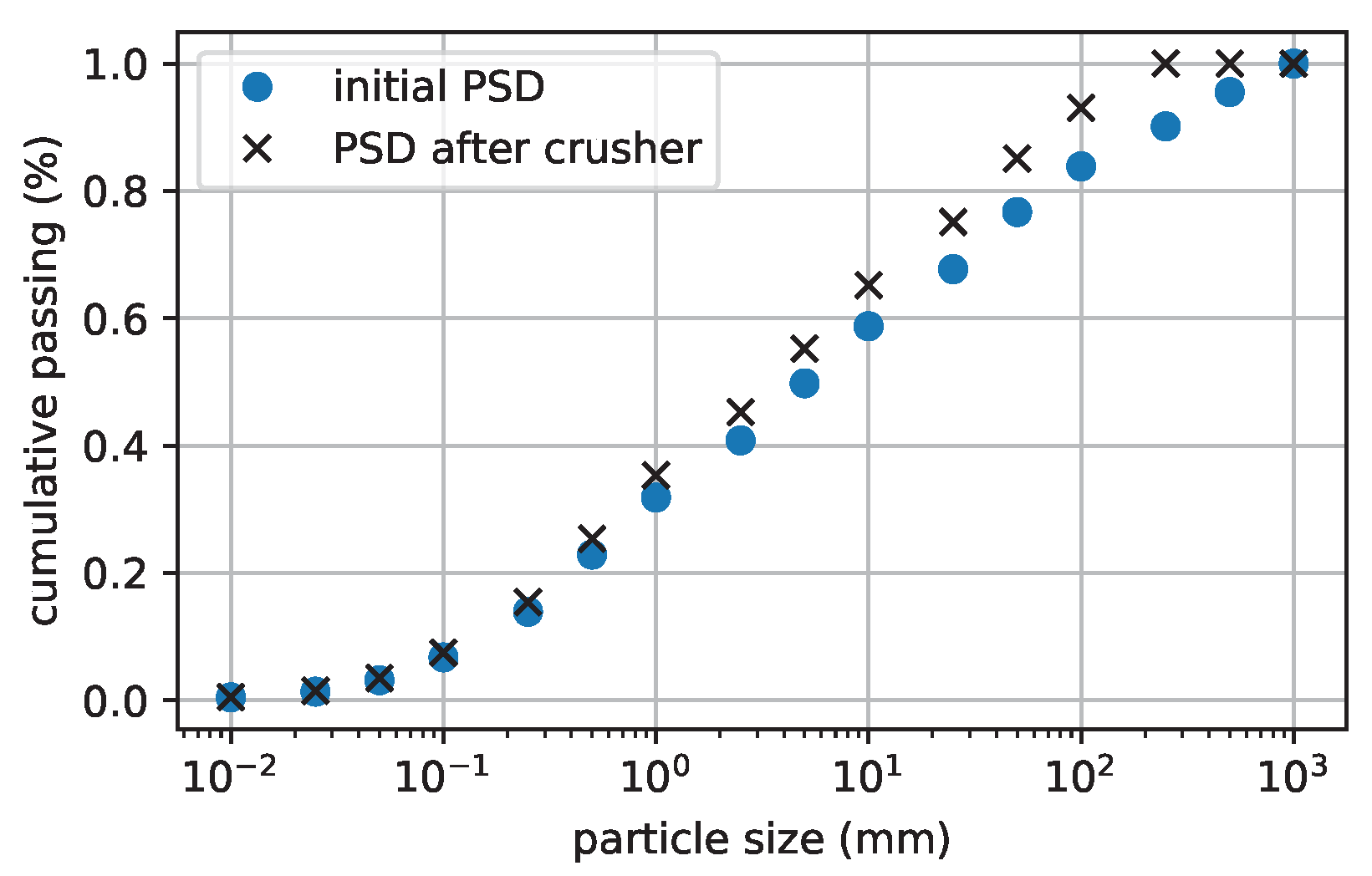
Macro-tracking events include the haul trucks dispatching from the loading point, dumping at the crusher station, material passing the crusher zone, the inlets and outlets to the stockpile and the inlet to the grinder. Model order reduction was applied on the belt conveyors. The simulator was implemented using the physics engine AGX Dynamics [29], using a nonsmooth (or time-implicit) DEM [17] for the particles and rigid multibody dynamics for the asset’s moving parts using feedforward controllers. The pseudo-particle size ranged between and m, which corresponded to a mass range between 12 and 160 kg. The distance between the two loading points was roughly 150 m, and the stockpile was 60 m tall. The simulations were run with a time-step of 11 ms and 100 projected Gauss–Seidel solver iterations, which corresponded to an error tolerance of around 5% for the stockpile bulk behaviour [17]. At the sources, each particle was assigned an identity and a location of origin. The left source was assigned a mineral concentration of , while the right source was assigned the value . The right source was given a mineral hardness of , while the hardness at the left source varied over the ore body according to some function . It was tested how a step in the hardness distribution function, from a value of to , in the left source propagated through the system. It was also investigated how well a hardness profile in the ore body could be backtracked from observations at the crusher and the grinder. The (true) particle size distribution was discretized in size classes with a logarithmic binning. The initial size distributions is shown in Figure 5, including also the average size distribution after the crusher. Note that the pseudo-particle diameter, used for visualization and contact dynamics, had no correspondence to its internal particle size distribution.
Each haul truck received a load of roughly 15 tons (roughly 150 pseudo-particles) at the loading point. For simplicity, the loading equipment was not modelled explicitly. The trucks dumped the load on the crusher inlet, and there, mixing of the material sources occurred from here on. The crusher was modelled as a jaw crusher, drawing material from above and crushing it with a jaw driven in an oscillatory motion. The pseudo-particles retained their original diameter, but when they passed the jaw, the internal particle size distribution was transformed. The fractions larger than the crusher gap width, m, broke into a uniform distribution of the smaller size classes. This unit operation was represented by , with the change vector for crushed (oversize) fractions, for (otherwise zero) and the change vector for the undersized fractions (otherwise zero). The resulting size distribution is shown in Figure 5. We assumed that the torque for driving the jaw crusher was in proportion to the amount of mass in the crusher zone , its hardness and size distribution, according to the following model:
where the crushing coefficient for the oversized and for the undersized. The momentaneous power draw of the crusher was computed by , where rad/s was the crusher speed.
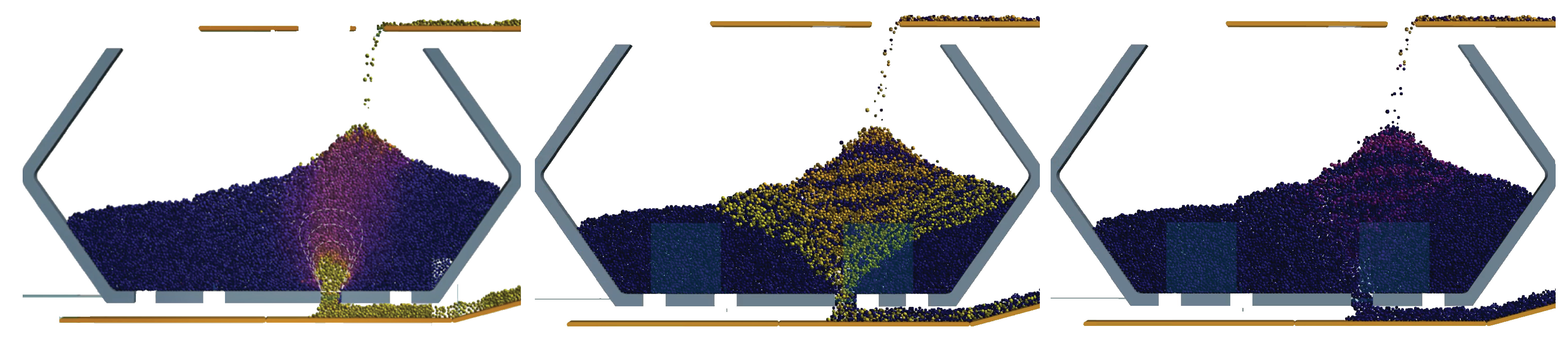
The stockpile held up to 2000 tons (roughly 20,000 pseudo-particles). There were two entry discharge points and four exit discharge points, but only one was used for the presented tests. When material was discharged from the bottom outlet, at a controlled speed ranging up to 2 m/s (or two tons/s), a funnel flow field was activated in the pile, reaching the surface where a depletion was gradually formed, unless new material was fed into the storage at the same rate or faster. Two time instances of pile states are shown in Figure 6. For the pointy pile state, one can expect more mixing of the incoming material and longer residence time, contrary to the depleted pile state where material flowed more directly through the storage and with less mixing.
An idealized mill model was assumed, guided by a model that was used for mill control at Boliden Aitik [30]. The idealized model consisted of a single grinder, although most real mills consist of a circuit of grinders and classifiers. When a pseudo-particle n reached the the grinder, a size reduction model began to operate on its size distribution. Each size fraction k was assigned a probability per unit time, , for breaking into smaller fractions and a probability per unit time, , for leaving the mill. At each time-step, the mass fractions carried by each pseudo-particle were redistributed according to , where the broken and passing fractions were:
and the reduced fractions were:
Modelling a size classifier, the probability per unit time for the finest fractions, smaller than , to leave the mill was . We used mm, and . The breakage probability depended on the (true) particle size, impact energy, hardness and the number of impacts [31], which in turn depended on the mill’s angular velocity, , and the active torque, . We assumed the following model for breakage probability per unit time:
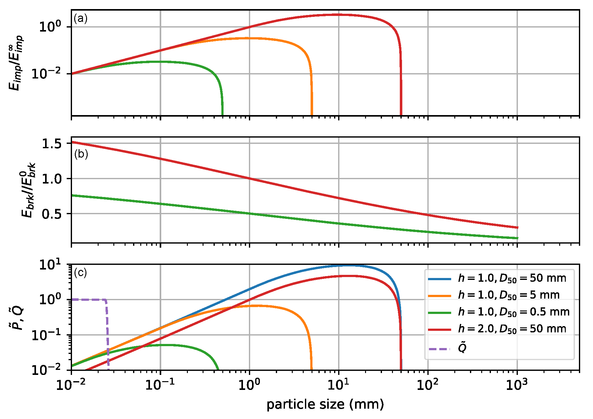
where is an impact energy distribution function, is a specific breakage energy distribution, is the (time-dependent) mean diameter of the material currently in the grinder, mm is a grinding length-scale parameter and a dimensionless breakage coefficient. The internal drive friction, , of an empty mill and the critical mill speed, rad/s, were used for normalization. The mill breakage model can be seen in Figure 7, with . The exit probability is also included.
The total grinding torque was the sum of three contributions, . The total mass, , was the mass of the moving part of the mill, kg, plus the mass of the material in the grinder, . The internal drive friction was modelled , and the torque required for accelerating the grinder was , where we denote the internal friction coefficient , gravity acceleration m/s and mill radius m. The active torque depended on the charge’s mass, , size distribution and dynamic angle, which depended on the mill angular velocity. We assumed, again guided by [30], that the active torque could be modelled with effective internal friction of the charge . Here, is the mass of the charge fractions larger than an active grinding size , with index . We used mm, which was in the 16 class size representation, and . With , the effective internal charge friction and active torque dropped to zero at and above the critical velocity. The power draw of the grinder was computed as . When nothing else was stated, the mill was run at constant nominal speed rad/s.
5. Results
5.1. Step Response
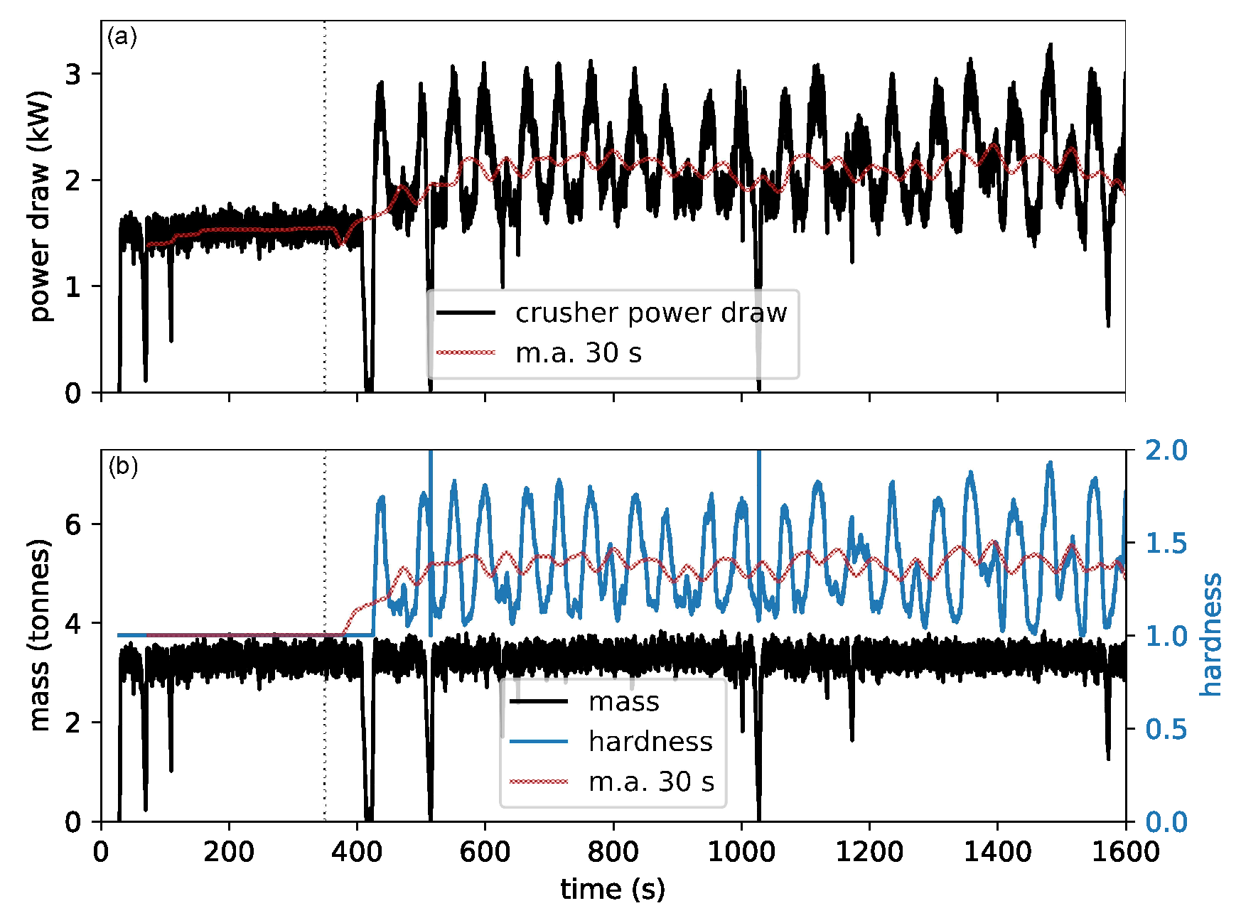
The simulator was initialized with ore of constant hardness transported from both sources. A step change to hardness was introduced at the left source, and the response in the crusher may be seen in Figure 8. The haul truck reached this harder material at time s. About 60 s later (five seconds more than one truck cycle), the crusher power draw increased by 40%, from kW to kW. A virtual sensor in the crusher revealed that the mineral hardness varied between one and two, with a time-averaged hardness around . The large oscillations in hardness and power draw, with a 55 s time period, was because of the trucks dumping interchangeably from the left and right source with hardness of one and two, respectively.
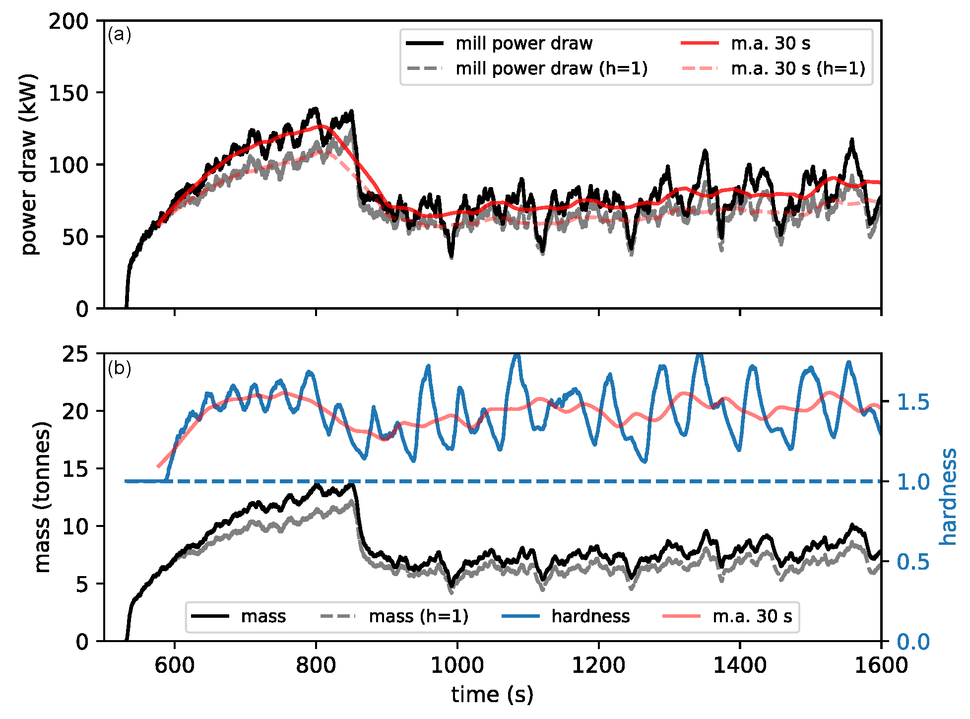
For the step response in the mill, we analysed the effect of the ore passing through the stockpile in Figure 6. The discharge of the piled material started at 500, and the feed reached the empty mill shortly thereafter. The material in the mill remained as hardness for 90 more seconds until it started increasing at time 590 s up to with only small oscillations (well mixed). At time 875 s, the storage level was down at zero (apart from the dead zones), and the rate of mass flowing into the mill dropped quickly to the rate of mass leaving the crusher and flowing into the storage. Therefore, after 875 s, the oscillations in hardness and power again reflected the truck cycles. For reference, we ran an identical simulation with constant hardness at both sources. As seen in Figure 9, the difference in the two power draw signals followed the increase in material hardness inside the mill. The increase was about 20% on average. Note that the mechanism for the higher power draw was that the harder ore took a longer time to grind, and the mill therefore accumulated more mass over time.
5.2. Identification of Hardness from Measurement-While-Drilling
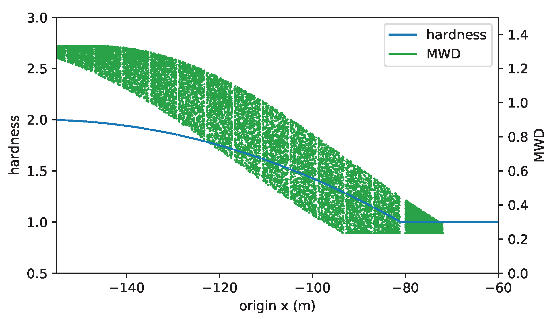
To test the feasibility of identifying the rock hardness from the MWD signal, we assumed the quadratic hardness profile in Figure 10 at the left source, ranging continuously between one and two. While drilling, a measurement profile was measured. For the test, we assumed and introduced a measurement location error such that , where is a uniform disturbance. We used m, which corresponded to six haul truck cycles back and forth to the crusher. The right source had constant hardness . Ore from the two sources entered the crusher, partially mixed, and gave rise to the torque signal in Figure 11.
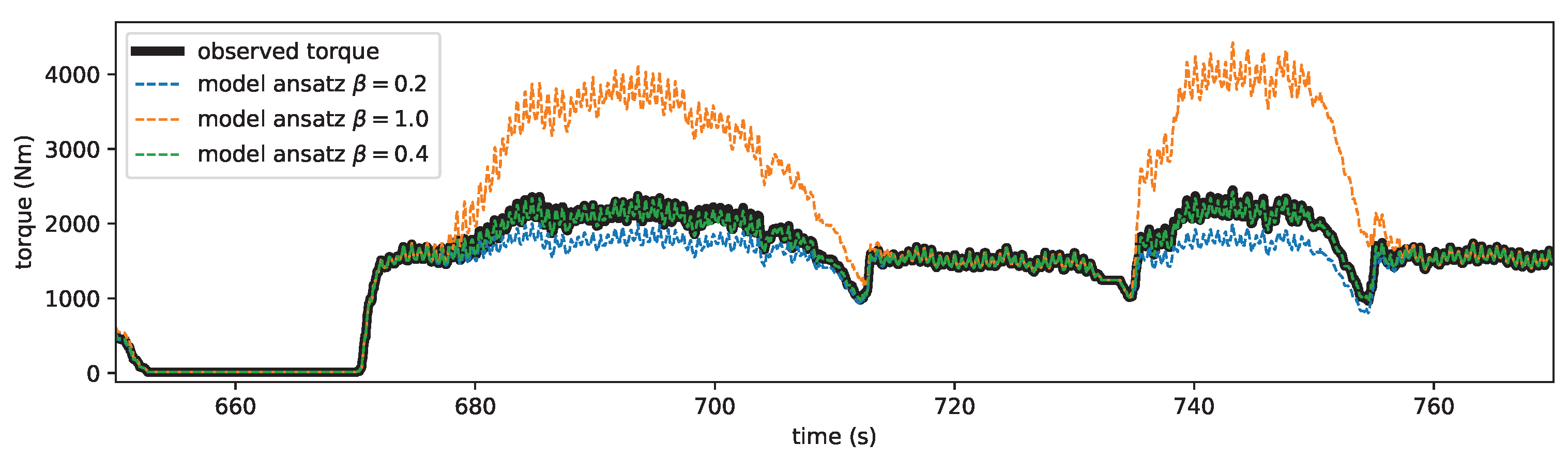
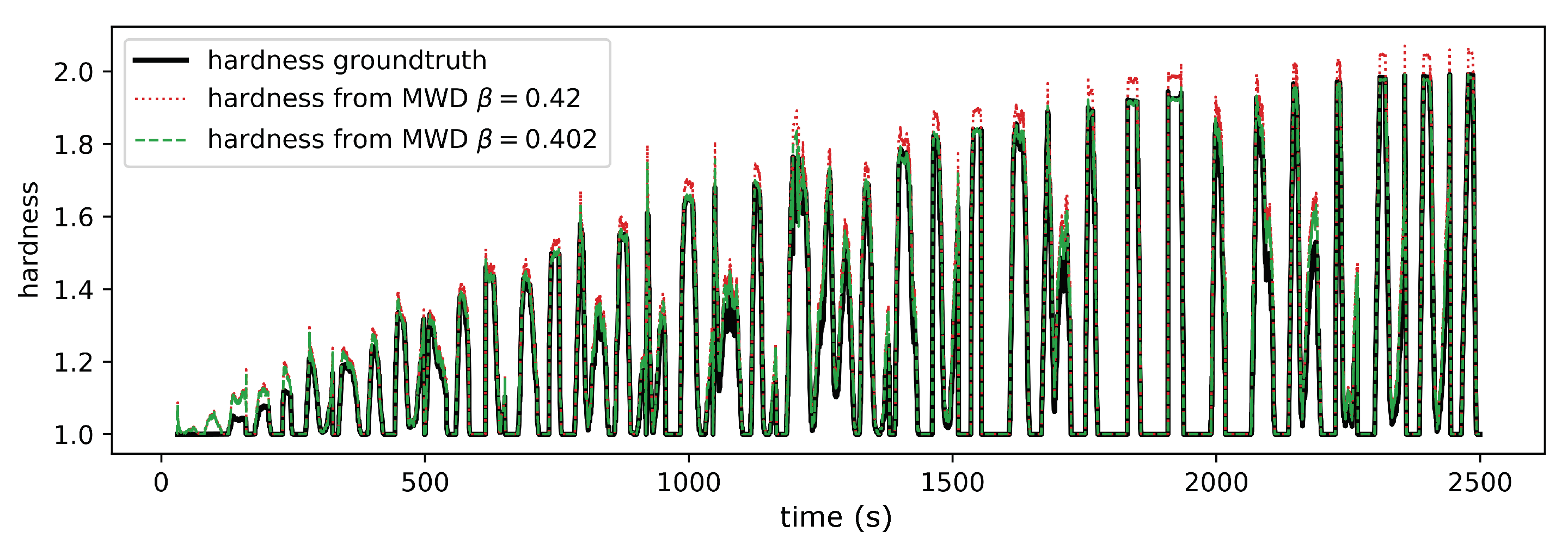
Assuming the crusher torque is related to rock hardness according to Equation (4), any ansatz can be explored and optimized with respect to model parameter . Different outcomes for the ansatz are shown in Figure 11. The best fit was found at , which deviated by % from the ground truth because of the tracking location error that was introduced. Note that empirical models between the ore tensile strength and adjusted drill penetration rate have this form in the literature [12]. Once a relation between the MWD signal and hardness was established, it was possible to predict the hardness of the material that was about to enter the crusher given the MWD signal measured at its location of origin. This is illustrated in Figure 12 over a sampling duration of 2500 s, or roughly 40 haul trucks from the left source.
5.3. Predicting the Properties of the Mill Feed
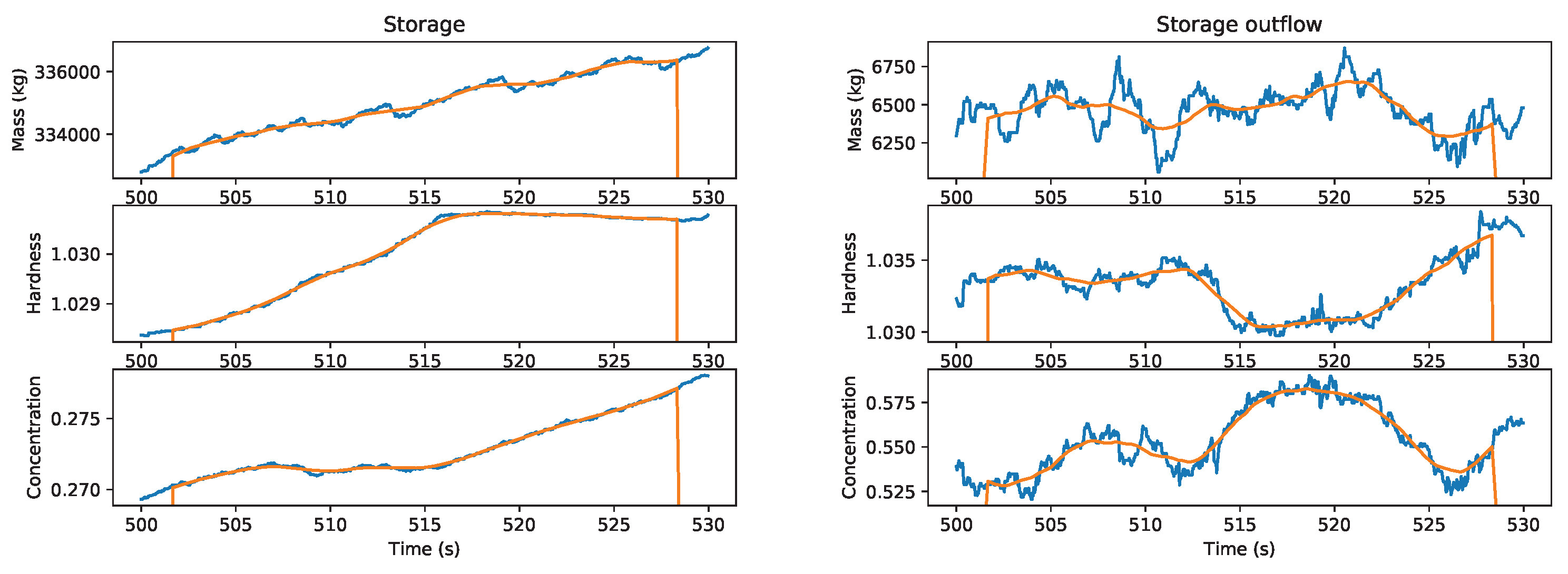
With particle-based tracking and Equation (3), it was straight-forward to monitor the properties of the ore kept in the storage as a function of time and space. Given a storage flow model, it was also possible to estimate which particles in the funnel zone would leave the storage in the near future, say the next 30 s. This way, the properties of the ore feed that would reach the mill could be predicted in advance, even before exiting the storage. Sample spatial distributions are shown in Figure 13. The time evolution of the properties in the pile and of the future feed are shown in Figure 14.
Backtracking the Grindability
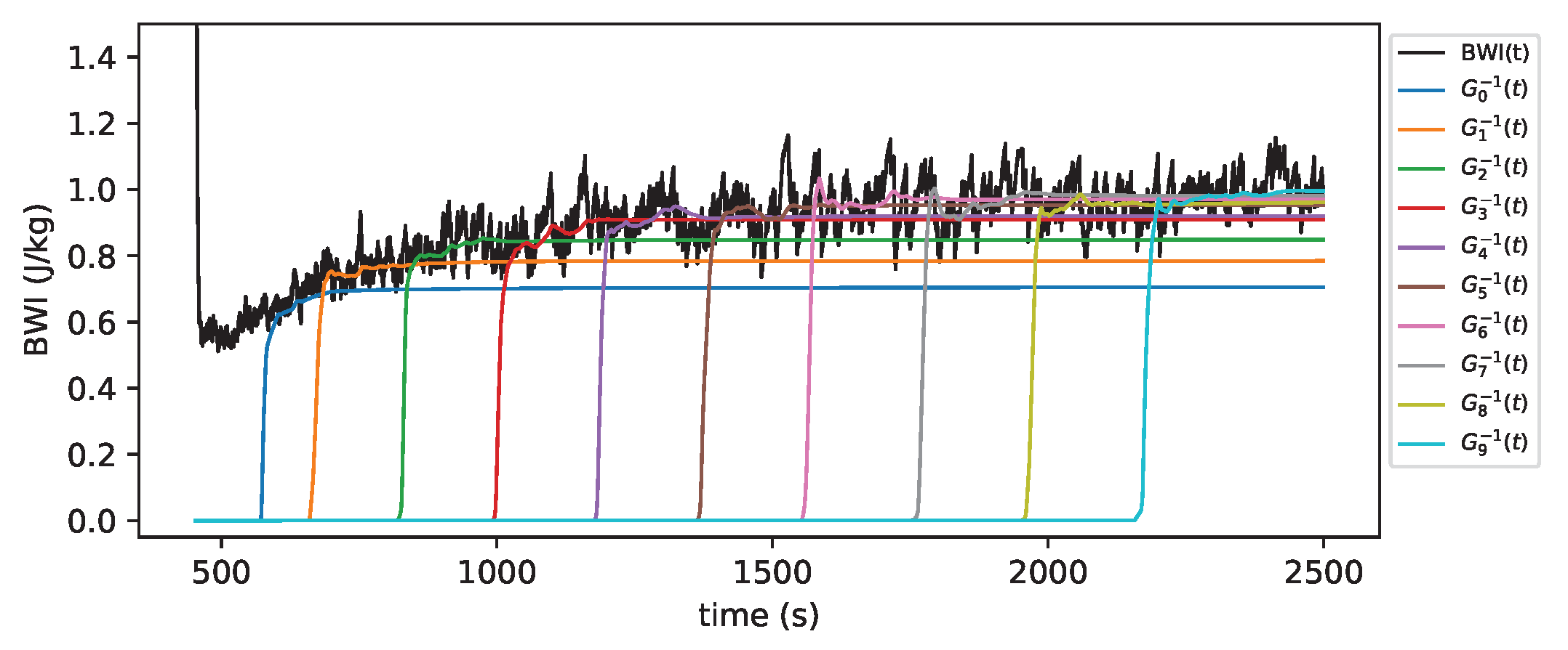
The grindability of an ore may be measured by the amount of energy, per unit mass, that is required for reducing the fragmentation down to a specific particle size. For the sake of production planning, the grindability is often estimated in advance using the relatively sparse exploration data of the ore body. The Bond ball mill work index (BWI) is defined as:
where the work per unit mass (W/kg) is computed as using a moving average with time-window . is the 80% passing diameter (m), computed from the cumulative size distribution function for mass that enters and leaves the mill. The bond grindability is then defined as the inverse . We demonstrated that the grindability measured in the mill can be backtracked to the ore’s location of origin for the purpose of improving future estimates for grindability. Assume there is an a priori, , estimate of the grindability of the ore in block i. At time , a grindability was observed at the mill. The average mass in the mill originating from the block i was . We reconciled the grindability at block i and time by the weighted average:
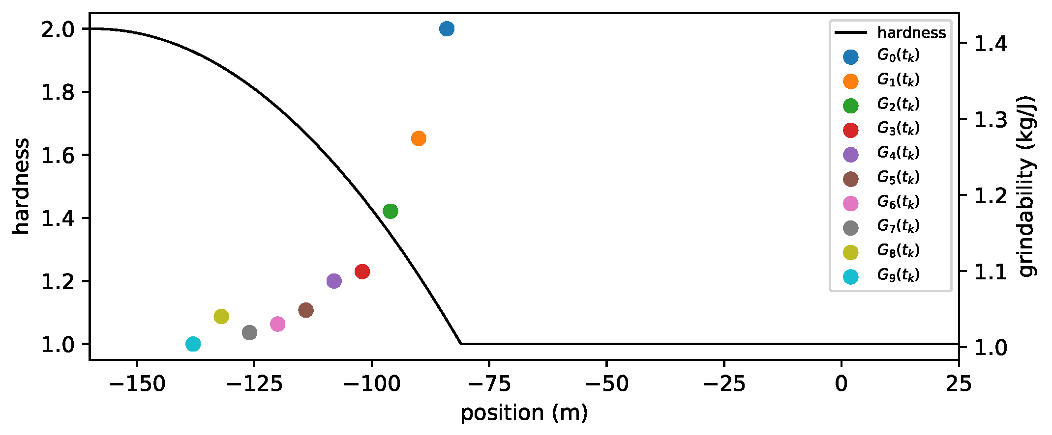
where the weight factor is given by the ratio of the mass with origin i to the mass in the mill and relative to the block mass . Here, is the amount of mass in the mill and is the total mass of the ore block i. Note that the weight factor is small (or zero) when there is little (or no) mass from the considered block. The weight factor for the original grindability reflects the confidence of that estimate, if the confidence is low and if the confidence is high. We tested backtracking the grindability of the ore originating from the left source for the case of a quadratic hardness profile shown in Figure 10, but mixed in the mill with ore from the right source. We used a block size of 10 m and . The BWI signals are shown in Figure 15, and the grindability backtracked to the source using Equation (9) is found in Figure 16.
6. Discussion
A digital twin of a mine may be realised as a system of particle simulations, distributed over virtual assets that evolve according to their physical counterparts using real-time particle simulation where no real sensors or control signals are available. This enables material tracking of ore from multiple sources passing through complex storage systems, such as stockpiles with multiple inlets and discharge outlets. Material tracking is necessary for understanding how the mill performance depends on natural variations in the raw material at the different sources and on the actions taken at drilling, blasting and crushing.
A concrete application example is to optimise the mill’s throughput energy consumption by controlling the fragmentation of the ore in relation to its hardness, known as mine-to-mill optimisation. It is widely accepted that energy savings up to 30% can be obtained by doing so [32]. First, the grindability of the ore body must be understood, by measuring the energy consumption in the mill and back-tracking it to the source. The next step is to determine how the grindability depends on the fragmentation and hardness of the material. The latter can be predicted from MWD data in combination with exploration data [12]. An optimal target fragmentation can then be predicted given the local material properties and realised by a specific drill and blast plan. The next level of optimisation is to control the stockpile flow so that the mill feed maintains an even and high grindability or pre-emptive regulation of the grinder in cases where variations are unavoidable. In [33], a 60% increase in the plant throughput was achieved this way, by using physical tracers to track the material from different sources to the mill via crushers and storages. That is, however, not sustainable over time, and a digital tracking system must be used in place.
This application puts a number of requirements on the digital material model used for tracking the material through the stockpile. To resolve the flow from different sources, the pseudo-particles must at least be smaller than a truck load. When the material lands on the stockpile surface, it is dispersed, which requires yet smaller pseudo-particles. The dispersion depends on the current shape of the pile surface, which may be complex when there are multiple discharge outlets, and on the material properties. When material is drawn, a flow channel develops, forming an inverted cone at the surfaces. If the incoming flow lands directly on the inverted cone, there is little dispersion, but if it lands on a slope or a conical top, the dispersion may be large: this is why a first-in-first-out or perfect mixing models is not suitable. Consequently, a grinder may at any time contain ore from many different trucks, and its content needs to be discretized sufficiently. Assuming the mill has a significant contribution of mass from 100 different trucks, thanks to dispersion and mixing in the stockpile, the mill mass must be resolved with at least 1000 pseudo-particles. For a medium-sized SAG mill, that implies a particle size less than m. A medium-sized haul truck is then resolved by more than 100 particles that may disperse on the pile. This size is also small enough to pass through a stockpile outlet and resolve the funnel flow in the pile.
There are a number of uncertainties to consider. The shape of the stockpile surface needs to be captured sufficiently. This can be done using the pseudo-particle model alone or by combining it with online measurements of the surface height to prevent the model drifting away from the true state. The particle contact parameters should be calibrated such that the dispersion over the surface is captured. This can be performed in advance using small test piles of the real material. The model for the funnel flow needs to be verified and calibrated. A measurement campaign with physical traces is the recommended way, measuring the residence time for each tracer and the evolving shape of the pile surface. In a cold climate, it might be necessary to carry this out several times to capture the temperature effect on the size of the dead zones and funnel flow, especially for temperatures below the freezing point. One limitation with the pseudo-particle model is that it does not automatically support size segregation effects, which may be significant when material is dispersed on a pile. The sieving mechanism makes large particles slide and roll further down the material bed than small ones. This can be dealt with by giving the pseudo-particles different internal size distributions and masses (maintaining the net size distribution and mass) and giving coarse and fine pseudo-particles different sizes and contact parameters such that the segregation effect evolves naturally.
Supplementary Materials
The following are available online at https://0-www-mdpi-com.brum.beds.ac.uk/article/10.3390/min11050524/s1, Video S1: Mine simulator, and Video S2: Integration test.
Author Contributions
Conceptualization, M.S.; data curation, F.V.; formal analysis, M.S. and F.V.; methodology, M.S., F.V. and E.W.; software, F.V. and E.W.; writing—original draft preparation, M.S.; writing—review and editing, M.S., F.V. and E.W. All authors have read and agreed to the published version of the manuscript.
Funding
The project was funded in part by eSSENCE and VINNOVA (Grant id 2019-04832). The computations were enabled by resources provided by the Swedish National Infrastructure for Computing (SNIC) at HPC2N, partially funded by the Swedish Research Council through Grant Agreement No. 2018-05973.
Institutional Review Board Statement
Not applicable.
Informed Consent Statement
Not applicable.
Data Availability Statement
Not applicable.
Acknowledgments
The authors are grateful for the support by ABB and Algoryx Simulation in carrying out the demonstration and integration tests and to Boliden and Epiroc for providing background information about mine-to-mill challenges, MWD data and the role of material tracking.
Conflicts of Interest
The funders had no role in the design of the study; in the collection, analyses, or interpretation of data; in the writing of the manuscript, or in the decision to publish the results.
References
- Holmberg, K.; Kivikytö-Reponen, P.; Härkisaari, P.; Valtonen, K.; Erdemir, A. Global energy consumption due to friction and wear in the mining industry. Tribol. Int. 2017, 115, 116–139. [Google Scholar] [CrossRef]
- Radziszewski, P. Energy recovery potential in comminution processes. Miner. Eng. 2013, 46–47, 83–88. [Google Scholar] [CrossRef]
- McKee, I. Understanding Mine to Mill; The Cooperative Research Centre for Optimising Resource Extraction (CRC ORE): Kenmore, Australia, 2013. [Google Scholar]
- Grieves, M. Digital twin: Manufacturing excellence through virtual factory replication. White Pap. 2014, 1, 1–7. [Google Scholar]
- Jeschke, S.; Brecher, C.; Meisen, T.; Özdemir, D.; Eschert, T. Industrial internet of things and cyber manufacturing systems. In Industrial Internet of Things; Springer: Berlin, Germany, 2017; pp. 3–19. [Google Scholar]
- Rossi, M.; Deutsch, C. Mineral Resource Estimation; Springer: Berlin, Germany, 2014. [Google Scholar]
- Ouchterlony, F.; Sanchidrián, J. A review of development of better prediction equations for blast fragmentation. J. Rock Mech. Geotech. Eng. 2019, 11, 1094–1109. [Google Scholar] [CrossRef]
- Evertsson, M. Cone Crusher Performance. Ph.D. Thesis, Chalmers University of Technology, Göteborg, Sweden, 2000. [Google Scholar]
- Napier-Munn, T.; Morrell, S.; Morrison, R.; Kojovic, T. Mineral Comminution Circuits Their Operation and Optimisation; Julius Kruttschnitt Mineral Research Centre, University of Queensland: Indooroopilly, Australia, 1996. [Google Scholar]
- Rai, P.; Schunnesson, H.; Lindqvist, P.A.; Kumar, U. Measurement-while-drilling technique and its scope in design and prediction of rock blasting. Int. J. Min. Sci. Technol. 2016, 26, 711–719. [Google Scholar] [CrossRef]
- Zhou, H.; Hatherly, P.; Ramos, F.; Nettleton, E. An adaptive data driven model for characterizing rock properties from Drilling data. In Proceedings of the 2011 IEEE International Conference on Robotics and Automation, Shanghai, China, 9–13 May 2011; pp. 1909–1915. [Google Scholar]
- Park, J.; Kim, K. Use of drilling performance to improve rock-breakage efficiencies: A part of mine-to-mill optimization studies in a hard-rock mine. Int. J. Min. Sci. Technol. 2020, 30, 179–188. [Google Scholar] [CrossRef]
- Singh, S.P.; Narendrula, R. Factors affecting the productivity of loaders in surface mines. Int. J. Min. Reclam. Environ. 2006, 20, 20–32. [Google Scholar] [CrossRef]
- Khorzoughi, M.B.; Hall, R. Diggability assessment in open pit mines: A review. Int. J. Min. Miner. Eng. 2016, 7, 181–209. [Google Scholar] [CrossRef]
- Brunton, I.D.; Thornton, D.M.; Hodson, R.; Sprott, D. Impact of blast fragmentation on hydraulic excavator dig time. In Proceedings of the Fifth Large Open Pit Conference, Kaalgorlie, Australia, 3–5 November 2003. [Google Scholar]
- Kvarnström, B.; Bergquist, B. Improving traceability in continuous processes using flow simulations. Prod. Plan. Control 2012, 23, 396–404. [Google Scholar] [CrossRef]
- Servin, M.; Wang, D.; Lacoursiére, C.; Bodin, K. Examining the smooth and nonsmooth discrete element approaches to granular matter. Int. J. Numer. Meth. Eng. 2014, 97, 878–902. [Google Scholar] [CrossRef]
- Wallin, E.; Servin, M. Data-driven model order reduction for granular media. Comput. Part. Mech. 2021. [Google Scholar] [CrossRef]
- Erkayaoğlu, M. A Data Driven Mine-to-Mill Framework For Modern Mines. Ph.D. Thesis, The University of Arizona, Tucson, AZ, USA, 2015. [Google Scholar]
- Erkayaoglu, M.; Dessureault, S. Improving mine-to-mill by data warehousing and data mining. Int. J. Min. Reclam. Environ. 2019, 33, 409–424. [Google Scholar] [CrossRef]
- Benndorf, J.; Buxton, M.W.N. Sensor-based real-time resource model reconciliation for improved mine production control—A conceptual framework. Min. Technol. 2016, 125, 54–64. [Google Scholar] [CrossRef] [Green Version]
- Innes, C.; Nettleton, E.; Melkumyan, A. Estimation and tracking of excavated material in mining. In Proceedings of the 14th International Conference on Information Fusion, Chicago, IL, USA, 5–8 July 2011; pp. 1–8. [Google Scholar]
- Innes, C. A Stochastic Method for Representation, Modelling and Fusion of Excavated Material in Mining. Ph.D. Thesis, University of Sydney, Sydney, Australia, 2015. [Google Scholar]
- Wambeke, T.; Elder, D.; Miller, A.; Benndorf, J.; Peattie, R. Real-time reconciliation of a geometallurgical model based on ball mill performance measurements—A pilot study at the Tropicana gold mine. Min. Technol. 2018, 127, 115–130. [Google Scholar] [CrossRef] [Green Version]
- Zhao, S. 3D Real-Time Stockpile Mapping and Modelling with Accurate Quality Calculation Using Voxels. Ph.D. Thesis, University of Adelaide, Adelaide, Australia, 2016. [Google Scholar]
- Berton, A.; Jubinville, M.; Hodouin, D.; Prévost, C.; Navarra, P. Ore storage simulation for planning a concentrator expansion. Miner. Eng. 2013, 40, 56–66. [Google Scholar] [CrossRef]
- ABB Ability System 800xA. Available online: https://new.abb.com/control-systems/system-800xa (accessed on 11 January 2021).
- OPC Foundation Unified Architecture. Available online: https://opcfoundation.org/about/opc-technologies/opc-ua/ (accessed on 11 February 2021).
- AGX Dynamics. Available online: https://www.algoryx.se/products/agx-dynamics (accessed on 29 March 2021).
- Araker, M.; Bostrom, J. Simulation and Control of the Grinding Circuit in Boliden Aitik; Technical Report; Boliden Mineral AB and Optimation AB: Newark, DE, USA, 2020. [Google Scholar]
- Bruchmüller, J.; van Wachem, B.; Gu, S.; Luo, K. Modelling discrete fragmentation of brittle particles. Powder Technol. 2011, 208, 731–739. [Google Scholar] [CrossRef]
- Napier-Munn, T. Is progress in energy-efficient comminution doomed? Miner. Eng. 2015, 73, 1–6. [Google Scholar] [CrossRef]
- Rybinski, E.; Ghersi, J.; Davila, F.; Linares, J.; Valery, W.; Jankovic, A.; Valle, R.; Dikmen, S. Optimisation and continuous improvement of Antamina comminution circuit. In Proceedings of the SAG Conference, Brisbane, Australia, 25–28 September 2011; Volume 19. [Google Scholar]
Figure 1.
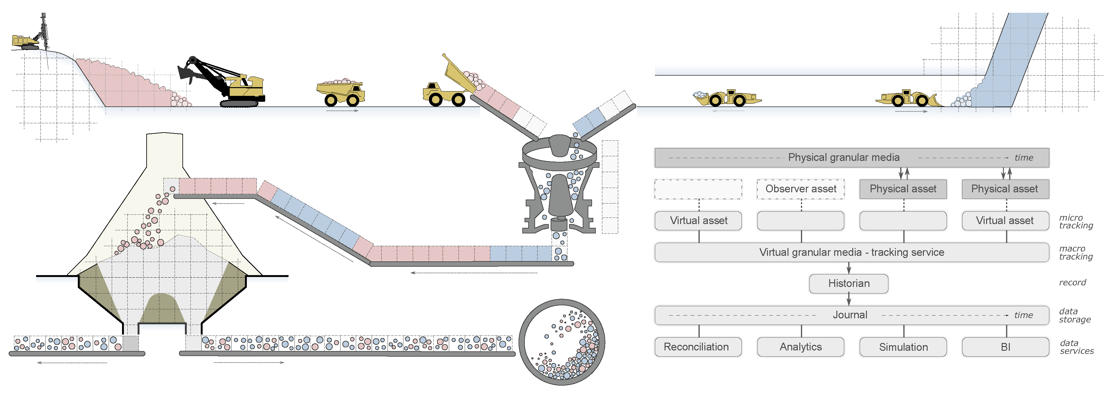
Illustration of a mine-to-mill process with particle-based material tracking. The chain of processes includes: drilling; blasting; load, haul and dump; conveying; crushing; sizing; storage and reclaim; and grinding; which then lead to a concentrator. The processes are carried out by physical assets that perform unit operations on the material. Connected virtual assets mirror the operations by transforming a distributed digital representation of the material. The architecture of the system of assets and services for tracking, data storage and analytics is illustrated in the lower right.
Figure 1.
Illustration of a mine-to-mill process with particle-based material tracking. The chain of processes includes: drilling; blasting; load, haul and dump; conveying; crushing; sizing; storage and reclaim; and grinding; which then lead to a concentrator. The processes are carried out by physical assets that perform unit operations on the material. Connected virtual assets mirror the operations by transforming a distributed digital representation of the material. The architecture of the system of assets and services for tracking, data storage and analytics is illustrated in the lower right.

Figure 2.
Illustration of micro- and macro-tracking. The sparse macro-tracking events include the appearance of fragmented material at the source (pink or blue) after blasting, haul truck asset dispatching and dumping (yellow), material entering later being discharged from a storage asset (green) and a conveyor asset (grey). The micro-tracking is the relatively high-frequency tracking of the material moving with or flowing inside an asset.

Figure 3.
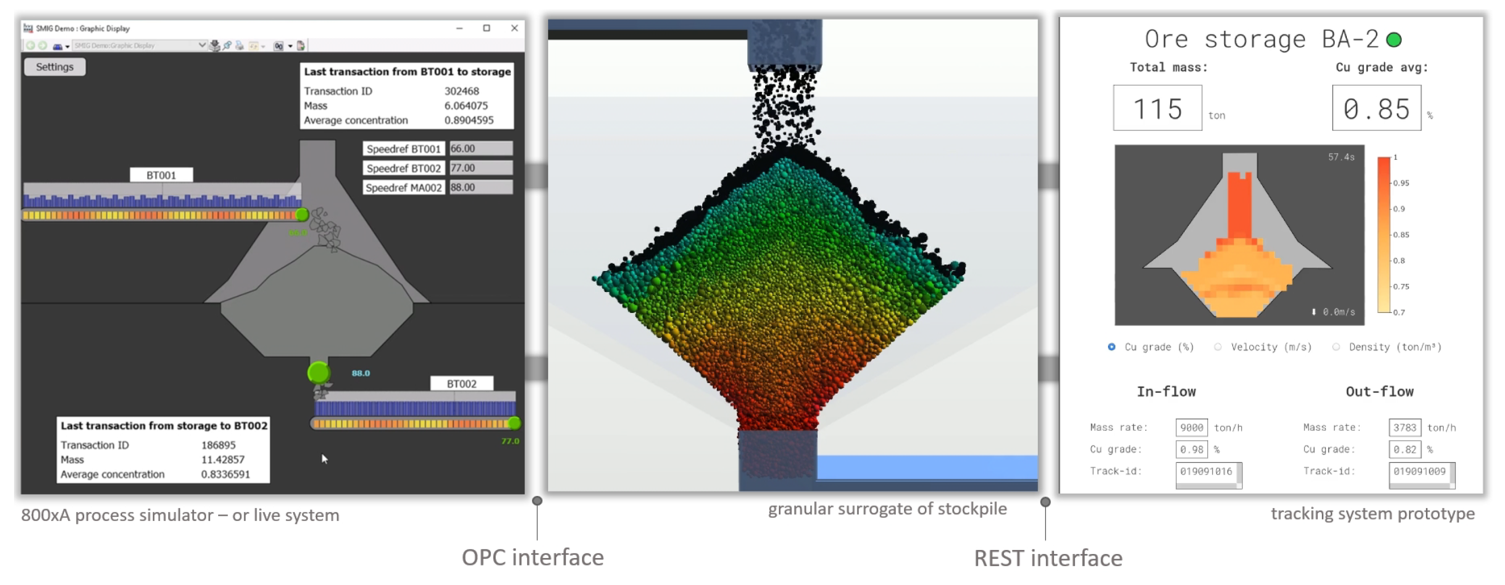
The integration test system includes two conveyor assets in an ABB 800xA simulator (left), a storage asset (centre) driven by a granular surrogate and a monitoring service (right) displaying macro-tracking data and virtual sensor data from the storage. The communication interfaces rely on OPC and REST, respectively. In the granular surrogate, black particles are dynamic, while the others are propagated using the reduced model and colour coded by residence time. A video is included as Supplementary Material Video S1.
Figure 3.
The integration test system includes two conveyor assets in an ABB 800xA simulator (left), a storage asset (centre) driven by a granular surrogate and a monitoring service (right) displaying macro-tracking data and virtual sensor data from the storage. The communication interfaces rely on OPC and REST, respectively. In the granular surrogate, black particles are dynamic, while the others are propagated using the reduced model and colour coded by residence time. A video is included as Supplementary Material Video S1.

Figure 4.
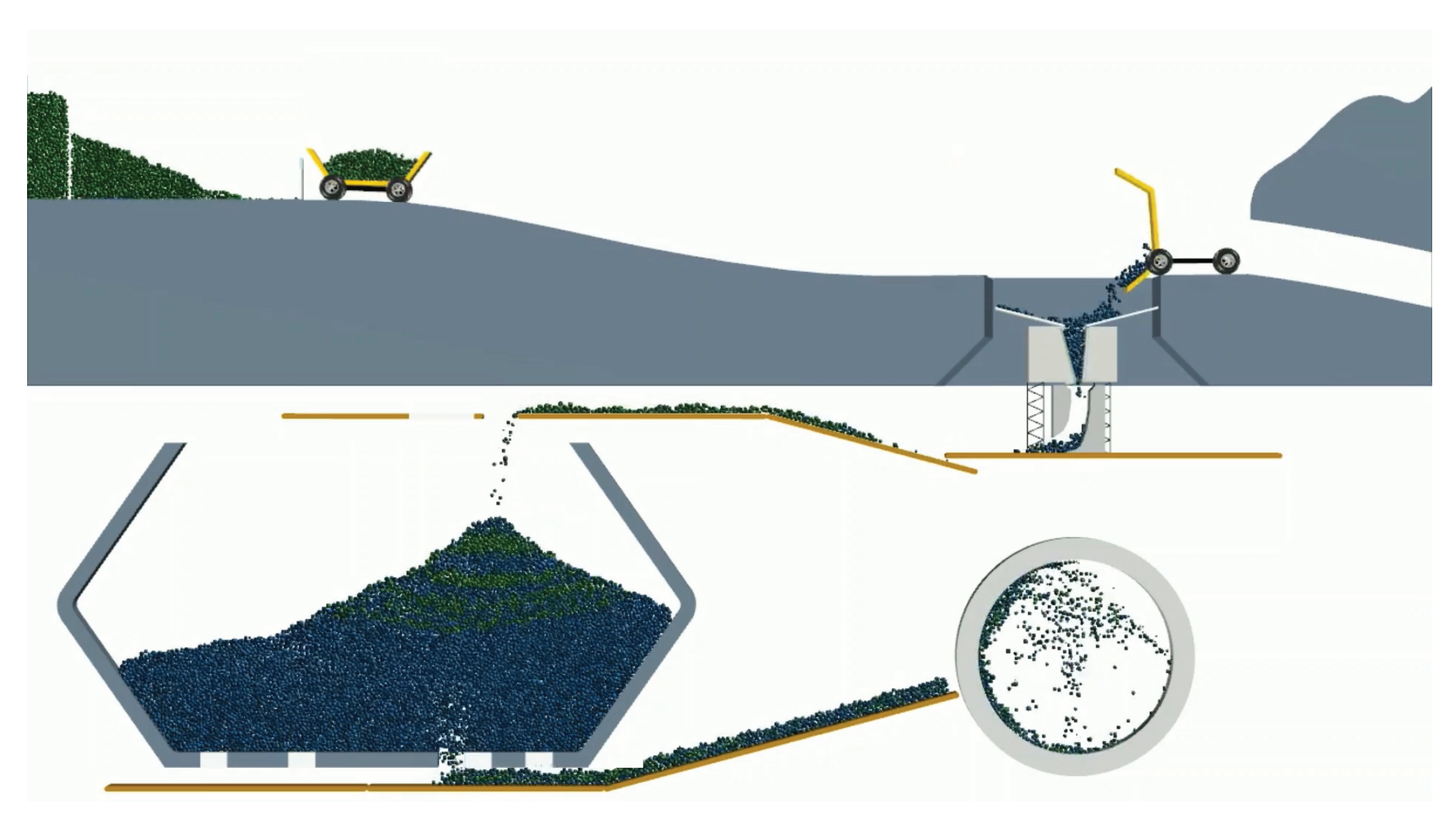
Image from the simulator with material hauled with trucks from two sources, dumped at a jaw crusher, conveyed to and from a storage and, finally, fed to a grinder. Green particles come from the left source and blue particles from the right source. A video is available as Supplementary Material Video S2.
Figure 4.
Image from the simulator with material hauled with trucks from two sources, dumped at a jaw crusher, conveyed to and from a storage and, finally, fed to a grinder. Green particles come from the left source and blue particles from the right source. A video is available as Supplementary Material Video S2.

Figure 5.
The cumulative particle size distribution (PSD) after blasting and after the crusher.

Figure 6.
The storage asset at two different pile states, pointy (a) and depleted (b). Blue and green particles have hardness values of 1 and 2, respectively.
Figure 6.
The storage asset at two different pile states, pointy (a) and depleted (b). Blue and green particles have hardness values of 1 and 2, respectively.

Figure 7.
The mill breakage model as a function of particle size and mineral hardness illustrated in terms of the impact energy distribution (a), specific breakage energy (b) and the breakage probability rate (c). The probability rate for exiting the mill is also included.
Figure 7.
The mill breakage model as a function of particle size and mineral hardness illustrated in terms of the impact energy distribution (a), specific breakage energy (b) and the breakage probability rate (c). The probability rate for exiting the mill is also included.

Figure 8.
The response in the crusher power draw (a) from a step change in the mineral hardness (b). Included are also 30 s moving averages, and the momentaneous mass in the crusher volume is also shown.
Figure 8.
The response in the crusher power draw (a) from a step change in the mineral hardness (b). Included are also 30 s moving averages, and the momentaneous mass in the crusher volume is also shown.

Figure 9.
The response in the mill power draw (a) from a step change in the ore hardness (b) after passing through the storage in Figure 6. The ore mass in the mill is also included and a 30 s moving average of the power draw and hardness. For reference, the case of constant hardness () is also included.

Figure 10.
The assumed hardness profile (blue) at the left source and the corresponding MWD signal (green) after introducing a 12.5 m measurement location error at the source.
Figure 10.
The assumed hardness profile (blue) at the left source and the corresponding MWD signal (green) after introducing a 12.5 m measurement location error at the source.

Figure 11.
Comparison between the observed crusher torque and the expected torque for different model parameters of the ansatz for the MWD–hardness relation. When the deviation is small (), the model is calibrated. In the presented period, four truck loads reach the crusher, two from the left source with harder ore and two from the right source.

Figure 12.
The true and predicted hardness given the MWD signal with the presence of a m tracking error. In addition to the best fit model (), a slightly erroneous fitted model () is included.
Figure 12.
The true and predicted hardness given the MWD signal with the presence of a m tracking error. In addition to the best fit model (), a slightly erroneous fitted model () is included.

Figure 13.
The spatial distribution of velocity (left), concentration (centre) and hardness (right) in the pile at a time instant. The material that will be discharged in the near future may be estimated from the funnel flow zone (left).
Figure 13.
The spatial distribution of velocity (left), concentration (centre) and hardness (right) in the pile at a time instant. The material that will be discharged in the near future may be estimated from the funnel flow zone (left).

Figure 14.
Evolution of the storage average properties over time (left) and the predicted feed for the next 30 s (right) given the funnel flow zone in Figure 13. A 2 s moving average is included (orange).
Figure 14.
Evolution of the storage average properties over time (left) and the predicted feed for the next 30 s (right) given the funnel flow zone in Figure 13. A 2 s moving average is included (orange).

Figure 15.
Time evolution of the bond ball mill work index (BWI) measured in the mill with material from both sources. The evolution of the backtracked (inverse) grindability at 10 individual blocks at the left source is also shown. The variations in power draw and hardness with a 55 s time period match the frequency of the truck hauling from the left source.

Figure 16.
The backtracked grindability at 10 individual blocks at the left source shown together with the hardness profile. As can be expected, these are inversely related.
Figure 16.
The backtracked grindability at 10 individual blocks at the left source shown together with the hardness profile. As can be expected, these are inversely related.

Publisher’s Note: MDPI stays neutral with regard to jurisdictional claims in published maps and institutional affiliations. |
© 2021 by the authors. Licensee MDPI, Basel, Switzerland. This article is an open access article distributed under the terms and conditions of the Creative Commons Attribution (CC BY) license (https://creativecommons.org/licenses/by/4.0/).
Share and Cite
MDPI and ACS Style
Servin, M.; Vesterlund, F.; Wallin, E. Digital Twins with Distributed Particle Simulation for Mine-to-Mill Material Tracking. Minerals 2021, 11, 524. https://0-doi-org.brum.beds.ac.uk/10.3390/min11050524
AMA Style
Servin M, Vesterlund F, Wallin E. Digital Twins with Distributed Particle Simulation for Mine-to-Mill Material Tracking. Minerals. 2021; 11(5):524. https://0-doi-org.brum.beds.ac.uk/10.3390/min11050524
Chicago/Turabian StyleServin, Martin, Folke Vesterlund, and Erik Wallin. 2021. "Digital Twins with Distributed Particle Simulation for Mine-to-Mill Material Tracking" Minerals 11, no. 5: 524. https://0-doi-org.brum.beds.ac.uk/10.3390/min11050524
Note that from the first issue of 2016, this journal uses article numbers instead of page numbers. See further details here.