First Demonstration of Recognition of Manganese Crust by Deep-Learning Networks with a Parametric Acoustic Probe

Abstract

The quantitative evaluations of mineral resources and delineation of promising areas in survey regions for future mining have attracted many researchers’ interest. Cobalt-Rich manganese crusts (Mn-crusts), as one of the three significant strategic submarine mineral resources, lack effective and low-cost detection devices for surveying since the challenging distribution requires a high vertical and horizontal resolution. To solve this problem, we have built an engineering prototype parametric acoustic probe named PPPAAP19. With the echo data acquired by the probe, the interpretation of the accurate thickness information and the seabed classification using the deep learning network-based method are realized. We introduce the acoustic dataset of the minerals collected from two sea trials. Firstly, the preprocessing method and data augment strategy used to form the dataset are described. Afterward, the performances of several baseline approaches are assessed on the dataset, and the experimental results show that they all achieve high accuracy for binary classification. We find that the end-to-end approach for binary classification based on a 1D Convolution Neural Network has a comprehensive advantage. Such a demonstration validates the possibility of binary classification for recognizing the ferromanganese crust only in an acoustic manner, which may significantly contribute to the efficiency of the survey.

1. Introduction

Cobalt-rich manganese crusts (Mn-crusts), together with polymetallic nodules and polymetallic sulfides, are considered the three most significant strategic submarine mineral resources. They grow over millions of years by precipitation from the ambient seawater and occur throughout the Pacific on seamounts, ridges, and plateaus [1,2,3]. In particular, there are large Mn-crust deposits in the north-western Pacific Ocean and spread over several hundreds of square kilometers [4]. Crusts mainly form at water depths of approximately 400 to 4000 m on the outer summit region and flanks of seamounts, with the thickest and most cobalt-rich crusts occurring at depths of about 800 to 2500 m, which may vary on a regional scale [3,5]. Gravity processes, sediment cover, submerged and emergent reefs, and currents control the distribution and thickness of crusts on seamounts [5]. They are rich in copper, cobalt, nickel, platinum, manganese, thallium, tellurium, and other metals [3]. In particular, they contain the metallic element of cobalt, which has many excellent properties and is necessary for the industry. For example, nowadays, it is widely used to increase chip performance and plays a decisive role in the artificial intelligence field [6]. Since the demand for minerals and metals is rising, people are paying more attention to the cobalt resources in the deep ocean [6]. Although exploiting the deep-sea mineral of Mn-crusts has great economic value, these resources in the Pacific have so far remained unexploited, which is mainly due to political uncertainties regarding ownership of the oceans and problems associated with mapping and exploring techniques in deep-sea water [6]. Considering this, the International Seabed Authority (ISA) has entered 15-year contracts to explore the three minerals in the deep seabed with twenty-two contractors, including the China Ocean Mineral Resources Research and Development Association (COMRA) [6]. For the deep-sea minerals of Mn-crusts, according to the regulations of ISA, they have the exclusive right to explore an initial area of 3000 km² from 27 July 2012, and only a 1000 km² area is to be reserved for future mining. Accordingly, they need to explore the most prospective regions with abundant Mn-crust minerals using various techniques.

The quantitative evaluations of mineral resources and delineation of promising areas in survey regions for future mining have attracted the interest of many researchers. International scientists are examining the problem from different angles to find a better method to identify areas that are rich in mineral resources on seamounts [7]. Generally, the assessment can be realized with two kinds of methods, i.e., direct and indirect measurements. The direct method generally means pointwise sampling from dredges or core drilling. Dredging surveys, for example, are often used to survey the thickness of Mn-crusts [8]. However, its main disadvantage is that samples recovered using this method are often damaged, and the method is biased toward loose rocks and edges that are more likely to be snagged [8]. As for core drilling and sampling from ROVs, although they are considered effective when obtaining the thickness and elemental composition of the sample, it is very time consuming to obtain samples, and the spatial resolutions achieved are limited to just a few samples every kilometer [8]. In contrast, indirect measurement is a remote and primary measurement in actual marine surveying that can improve precision mineral resource estimation and reduce the cost of the survey.

There are many optical or acoustic detection devices, such as camera and laser mapping systems, multi-beam systems, side-scan systems, sub-bottom profiles, and other acoustic equipment. Acoustic detection is frequently realized since high-quality acoustic backscatter data can allow us to estimate the geological distribution of the minerals.

The phenomena of reflection together with refraction and scattering will occur when the acoustic wave arrives at the interface with different medium impedance. As validated in [9], the geo-acoustic properties of polymetallic crusts are correlated to their chemical composition. Many researchers focus on the backscatter intensity with different submarine sediment types, including backscatter data collection, processing, and analysis [4]. The relationship of backscatter intensity with factors such as the hardness and roughness of the seafloor [10,11] and grain size with a given incident angle [12] are carefully depicted. Machida et al. [13] attempted to evaluate the potential of a dense field of ferromanganese (Fe-Mn) nodules discovered on a seamount approximately 300 km east of Minamitorishima Island as a resource for critical metals and showed that spherical nodules 5–10 cm in diameter almost fully cover the region of high acoustic reflectivity. Usui and Okamoto [14] correlated acoustic remote sensing data with the surface geology and decipher the regional-scale distribution of crusts in relation to large-scale mass wasting that took place in the early Miocene or before, showing that only about 40% of the apparent “acoustic outcrop” represents actual ferromanganese crust coverage. Nakamura et al. [15] used sub-bottom profiler data to obtain the acoustic characterization of pelagic sediments, which indicated a primary target for future mining. Machida et al. [16] integrated multiple datasets from different sounders and the observation periods to provide visualization and quantitative estimations to the distribution of ferromanganese deposits. Besides, acoustic seabed classification is realized utilizing acoustic backscatter data combined with information on the seabed sediments. For example, Yang et al. [5] employed the backscatter data of multi-beam EM122 to identify the distributions of manganese nodules (Mn-nodules) with different abundances, cobalt-rich crusts, pelagic calcareous and clay sediments, etc. They established the qualitative and quantitative relationship between backscatter and nodules, crusts, and different sediments at a large scale. Berthold et al. [17] proposed a model for the automatic sediment type classification with the side-scan sonar data. Ma et al. [18] employed a multiple-scale model to predict the distribution of the different sediment grain sizes, avoiding the arbitrary selection of the spatial scale for explanatory variables.

We should mention that compared with Mn-nodules, the survey requirements of Mn-crusts are rather different since Mn-nodules’ distribution can be determined from the surface appearance and shape alone, thus leading to the accurate estimation from traditional survey methods [8]. For Mn-nodules that can be found in basins between 3500 m and 6000 m depth [19,20,21,22], indirect methods such as shipboard multi-beam [23,24], photogrammetry, and side-scan surveys [25,26,27] from autonomous underwater vehicles (AUVs) and remotely operated vehicles (ROVs) have been applied [8]. However, it is challenging to obtain accurate estimates of Mn-crust distributions due to their extremely uneven distribution and thin geometrical features. From the technical perspective, accurately estimating the thickness and recognizing the target type enable us to infer the resources of Mn-crust precisely.

Thickness, water depth, slope, coverage, metal concentration, abundance, area for exploration, and area for future mining are emphasized as important factors in the evaluation of cobalt-rich crusts [7]. Of all the Mn-crusts features, the crust thickness has the largest variation coefficient and contributes much more to spatial changes in mineral resources [7]. Therefore, regarding the aim of our work, many efforts have been made to design a new kind of parametric sonar that is economic, efficient, and performs well and develop an effective algorithm to obtain one of the critical factors of accurate thickness information. Although the principle tightly connected to such sonar is that we can measure Mn-crust thickness as long as the Mn-crusts and their substrates have different acoustic impedances [6], which is the same as other traditional sonars, the detection scale is rather different. The high requirement of vertical and horizontal resolution is taken into consideration because of the Mn-crust’s challenging distribution. The first generation of such sonar tools is called Programmable Phased Parametric Array Acoustic Probe 2017 (PPPAAP17), which has a mass of about 60 kg and has a separate processing unit (height: 468 mm, diameter: 311 mm) and a transmit–receive array (height:109 mm, diameter: 292 mm). With it, we successfully carried out two sea trials in the China Ocean 41Bth voyage and China Ocean 51st voyage and obtained accurate thickness estimation results compared with those of the dredged samples. In 2019, based on the acoustic echo data acquired in the experiment, we have optimized the sonar to have a mass of about 20 kg and an integrated processing unit and transmit–receive array (height: 200 mm, diameter: 200 mm), which is named Programmable Phased Parametric Array Acoustic Probe 2019 (PPPAAP19).

As we have successfully obtained the thickness information using PPPAAP19, our goal is to identify the Mn-crust by analyzing the acoustic echo data acquired by the device at a small scale compared with other traditional sonars. In 2020, we carried out a preliminary experiment based on several physical materials with similar acoustic properties with a ferromanganese crust and the sediments to evaluate the effectiveness of the recognition algorithm [28]. Currently, other researchers have not published any related applications regarding recognizing a ferromanganese crust with parametric acoustic sonar.

Knowledge of the Mn-crust is an important research topic in marine geology, marine environment, geochemistry, and paleoceanography, as well as other research areas. In particular, we should emphasize the concepts of and differences between the Mn-crust and ferromanganese crusts (FC) before we introduce our method. Cobalt-rich manganese crusts (Mn-crust), which also could be abbreviated as CRC, are considered a specific FC that includes a high or moderate amount of cobalt. Although a reasonable assessment of the Mn-crust resource of some areas is very important, we cannot determine the cobalt-rich part (or area) from an entire region distributing FC since we cannot quantify the cobalt composition of the crust. Therefore, in the following paragraphs, the processing algorithm could be applied to the general detection of FC instead of only cobalt-rich minerals. In contrast, NonFC represents the sediment or bedrock with no manganese crusts on the surface.

Our goal of recognizing FC from other materials belongs to the research area of underwater acoustic recognition at a much finer scale. Some researchers have realized the volumetric measurements of Mn-crusts using high-frequency subsurface sonar and a 3-D visual mapping instrument mounted on these vehicles [29,30]. Compared with their visual mapping method, we achieve the identification with only a parametric probe. After acquiring the echo data, a good result can be obtained since the classification can benefit from the strong capability of the deep learning networks. In recent years, many promising machine-learning classification approaches and deep-learning classification approaches have been employed for underwater target detection applications, such as underwater acoustic target recognition [31], seafloor sediment classification [32], and source depth prediction [33]. Neilsen et al. applied convolutional neural networks (CNNs) to predict the seabed type, source depth and speed, and the closest point of approach [33]. Politikos et al. presented an object detection approach that automatically detects seafloor marine litter in a real-world environment using a Region-based CNN [34]. Zhu et al. [35] proposed a DNN model based on multiple features with different weights to predict sediments of three types and a shipwreck. Based on these outperforming results, the deep-learning methods based on different features are evaluated for the FC classification in this paper. Based on the echo data acquired by the active parametric sonar of PPPAAP19, we focus on validating the possibility of binary classification for recognizing FC in an acoustic manner only. In this paper, we will compare the performances of several baseline methods to determine the appropriate one to realize real-time binary recognition.

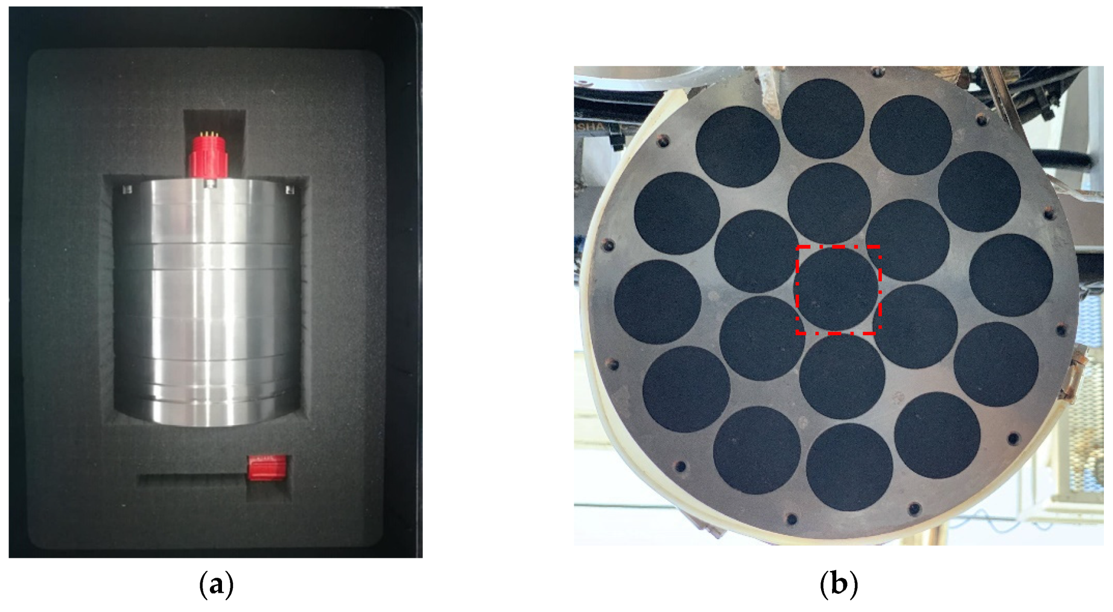
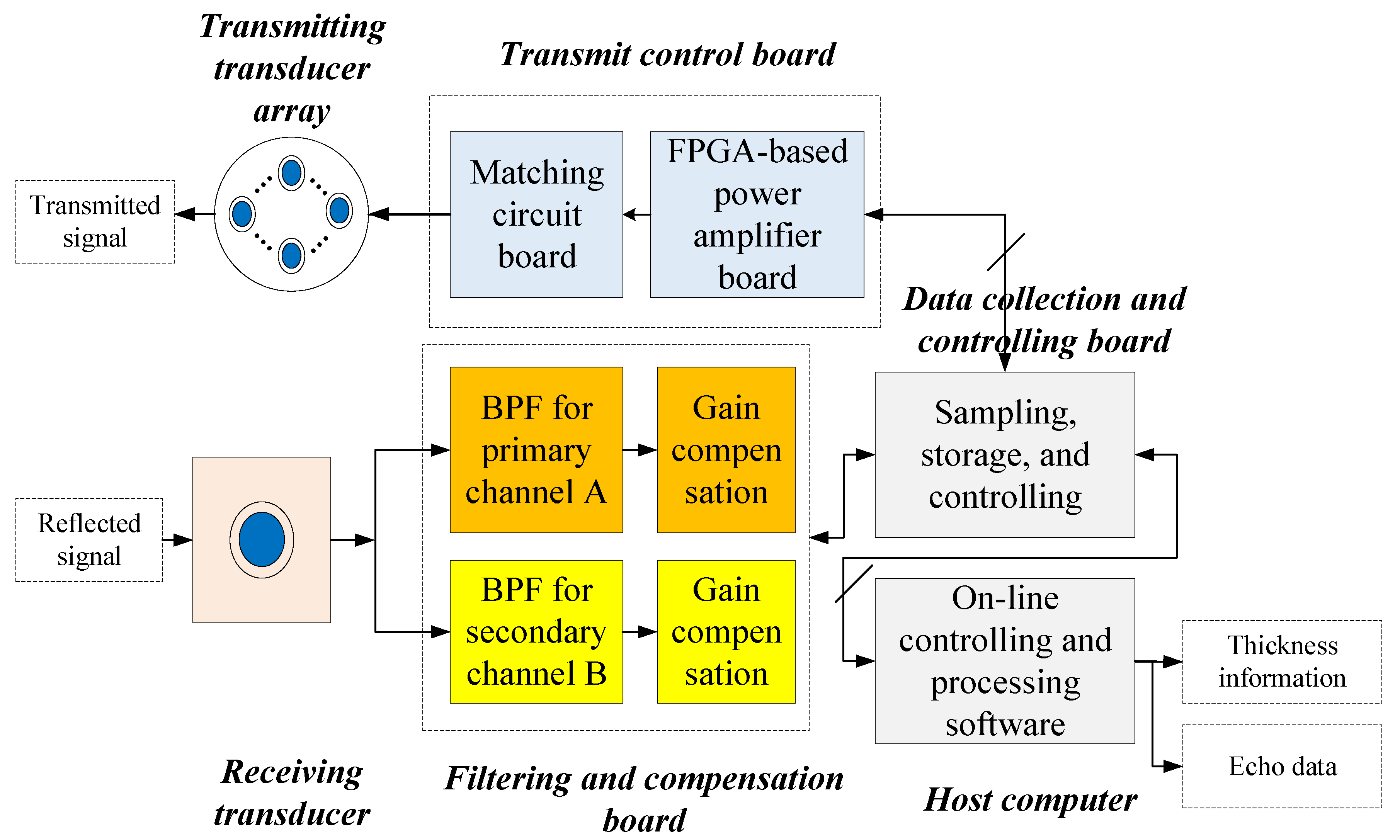
2. System Description

PPPAAP19 is designed to complete the task of remotely measuring the thickness of Mn-crusts that are within the range of 30 mm to 350 mm. Such a task requires the along-track and cross-track resolution to be high enough to detect the features between the Mn-crusts layers. Based on the parametric acoustic principle, the acoustic probe transmits a 1 MHz, high-frequency amplitude modulated signal to generate a narrow 100 kHz beam that penetrates the target [6]. PPPAAP19 is a sonar tool made of titanium alloy with a height of about 200 mm and a diameter of 200 mm, as shown in Figure 1a. The designed array is located at the bottom of the sonar tool with the receiving transducer marked with red and the other 18 transmitting transducers around it, as shown in Figure 1b. Compared with PPPAAP17, an elementary prototype [6], PPPAAP19 has better performance with reduced mass and volume.

As described in Figure 2, PPPAAP19 consists of one receiving transducer, two filtering and compensation boards, a transmitting array of 18 transducers, a transmit control board, and a data collection and controlling board. The transmitting parameters, such as the form of the transmitted signal, the independent control of each transducer, etc., can be set with the host computer and then transferred to PPPAAP19 [6]. The transmitting transducer array fires periodically while the receiving transducer receives the echo signal. The sampling rate of the primary signal and the secondary signal is 5 MHz and 2 MHz, respectively [6]. Afterward, the acoustic echo signal is filtered as the primary signal and secondary signal using two different Band Pass Filters (BPF), and the online controlling and processing software gives the real-time thickness estimation results with the signal-processing algorithm [6]. Meanwhile, the echo signal is recorded and used to recognize FC.

3. Binary Classification with Different Approaches

The motivation for developing a binary classifier of FC with the dual-channel signal based on deep learning networks is that the traditional feature-based classification approaches are limited by human design and are unsuitable for complex sea environments. We will compare different methods such as the 2D Convolutional Neural Networks with the feature of STFT (STFT+2D-CNN), Deep Neural Networks with the feature of FFT (FFT+DNN), and 1D Convolutional Neural Networks with the time-domain signal (Time-domain signal+1D-CNN). The flow of these binary classification methods consists of several steps, including dataset formation, feature extraction, and classifier design, as shown in Figure 3.

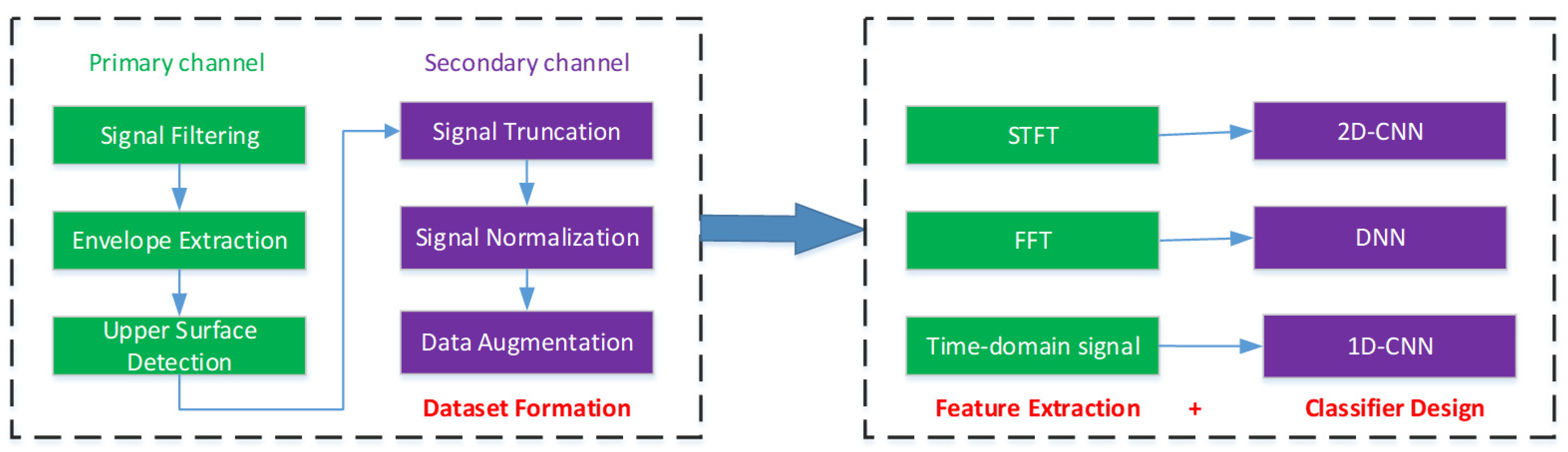
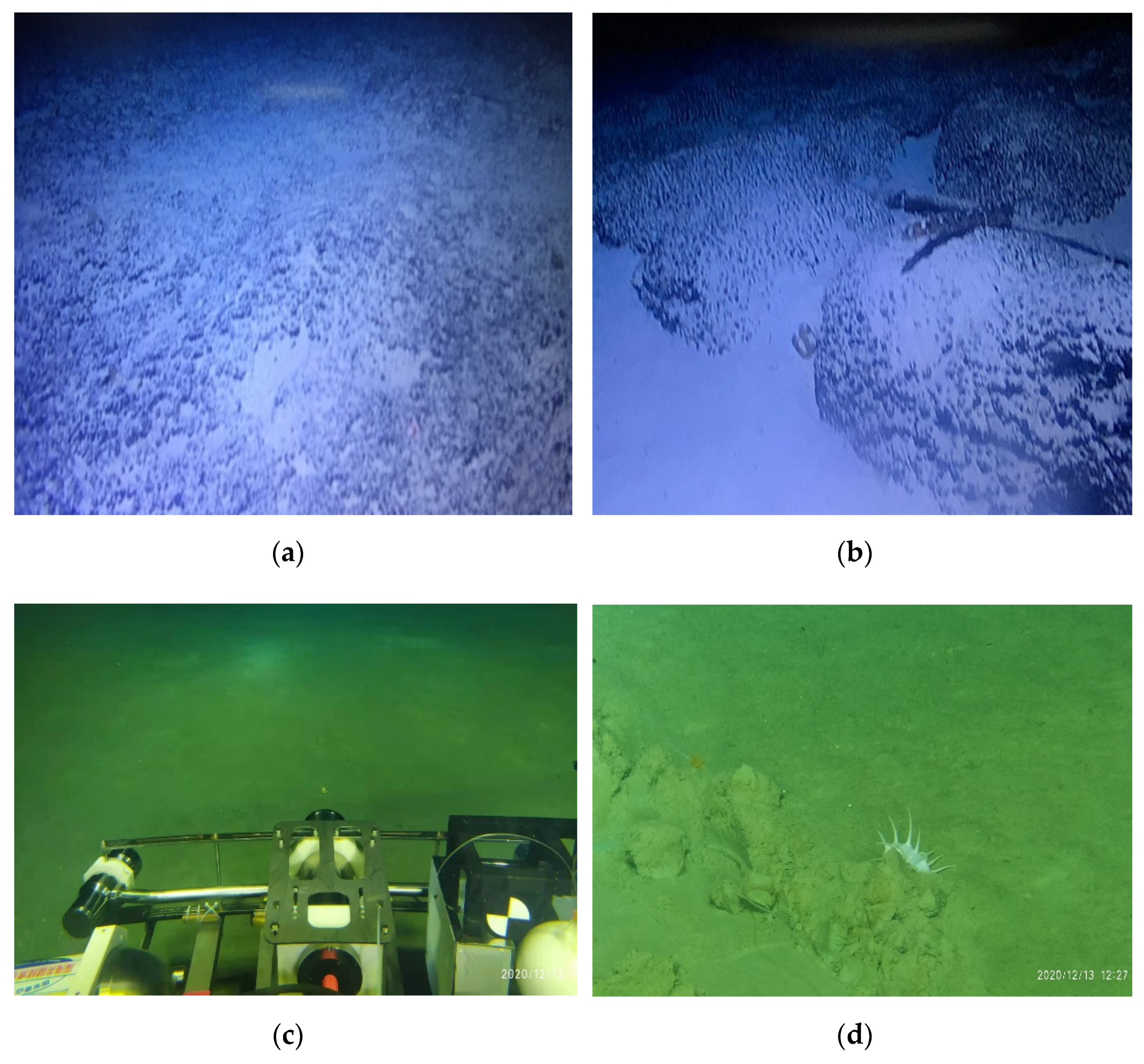
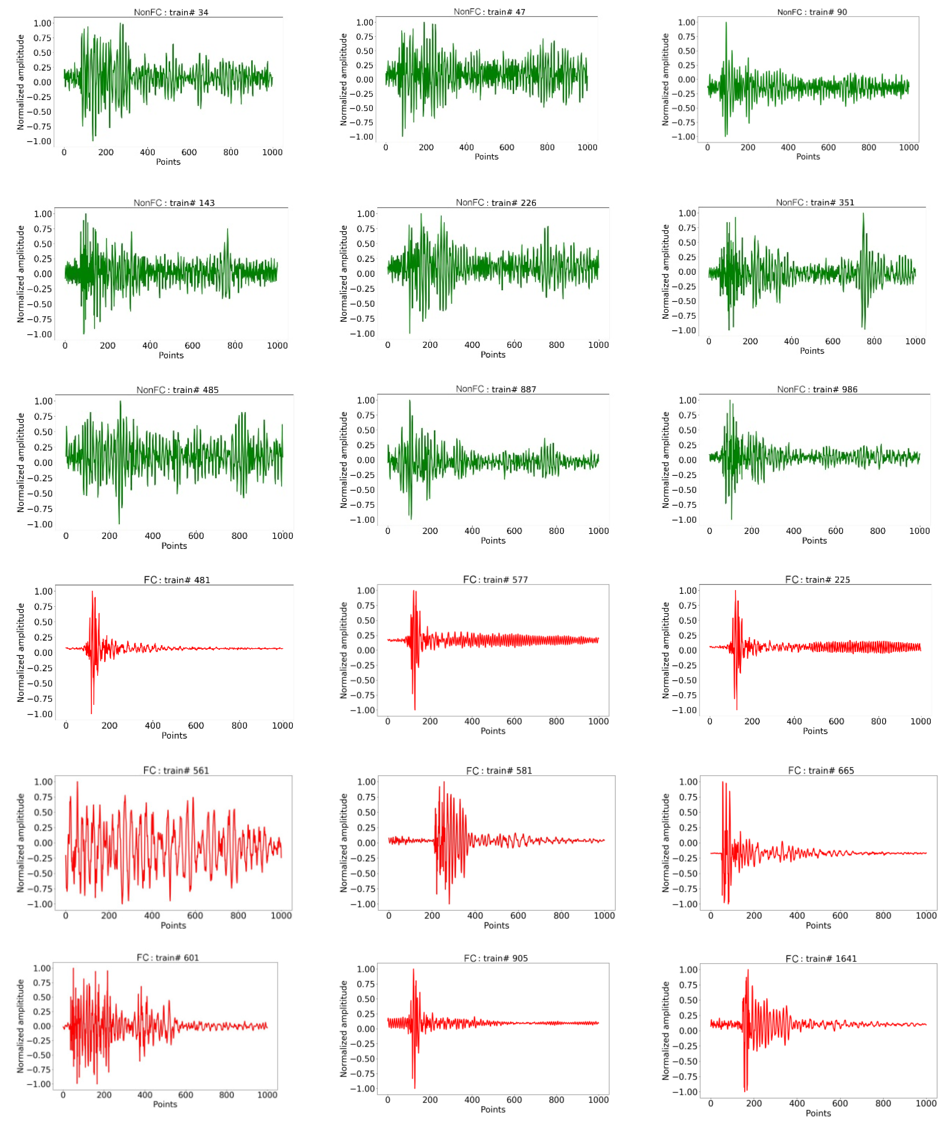
3.1. Dataset Formation

Let us first depict the idea of dataset formation. As the first step of preprocessing flow, automatic signal truncation is utterly essential. We could obtain the primary and secondary signals generated by the acoustic wave’s same propagating process within the seabed material for each record. However, since the recorded signal contains some interferences and blanket parts with a relatively long duration, we need to propose a method to extract the valuable part of the signal that contains only the necessary period that the acoustic wave propagates within the seabed material. As shown in Figure 3, signal filtering is the first step to filter the interference noise outside the bandwidth of the primary signal. After that, we extract the envelope of the primary signal with the Hilbert Transform. The reason behind it is that compared with the secondary signal, the peak position of the primary signal, which is regarded as the reflection that occurred at the upper surface, is more evident and precise due to its large Signal-to-Noise Ratio (SNR). Therefore, we find the peak time of the primary signal and convert it to the point of the peak time of the secondary signal according to their different sampling rate. Only a slice of the signal around the peak time is reserved, and the amplitude of the signal $s\left(t\right)$ can be normalized as,

$$x\left(t\right)=\frac{s\left(t\right)-\min \left(s\left(t\right)\right)}{\max \left(s\left(t\right)\right)-\min \left(s\left(t\right)\right)}$$

(1)

where $\max (\cdot )$ and $\min (\cdot )$ denote the maximum value and minimum value, respectively. Note that data normalization can accelerate the convergence speed of the network during training. Another important aspect relates to the proportion of the two classifications, which is unbalanced. Therefore, the signal with fewer samples needs to be augmented. The augmentation could be achieved by stretching the waveform in the time-domain, adding background noise, and adjusting audio pitch. We implement the augmentation by randomly adding Gaussian noise with different signal-to-noise ratios (SNR). Afterward, the new signal is filtered by a Butterworth filter with the same bandwidth as the preprocessed signal. Then, we can form the dataset of the secondary signal with the balanced types.

3.2. Description of Different Methods

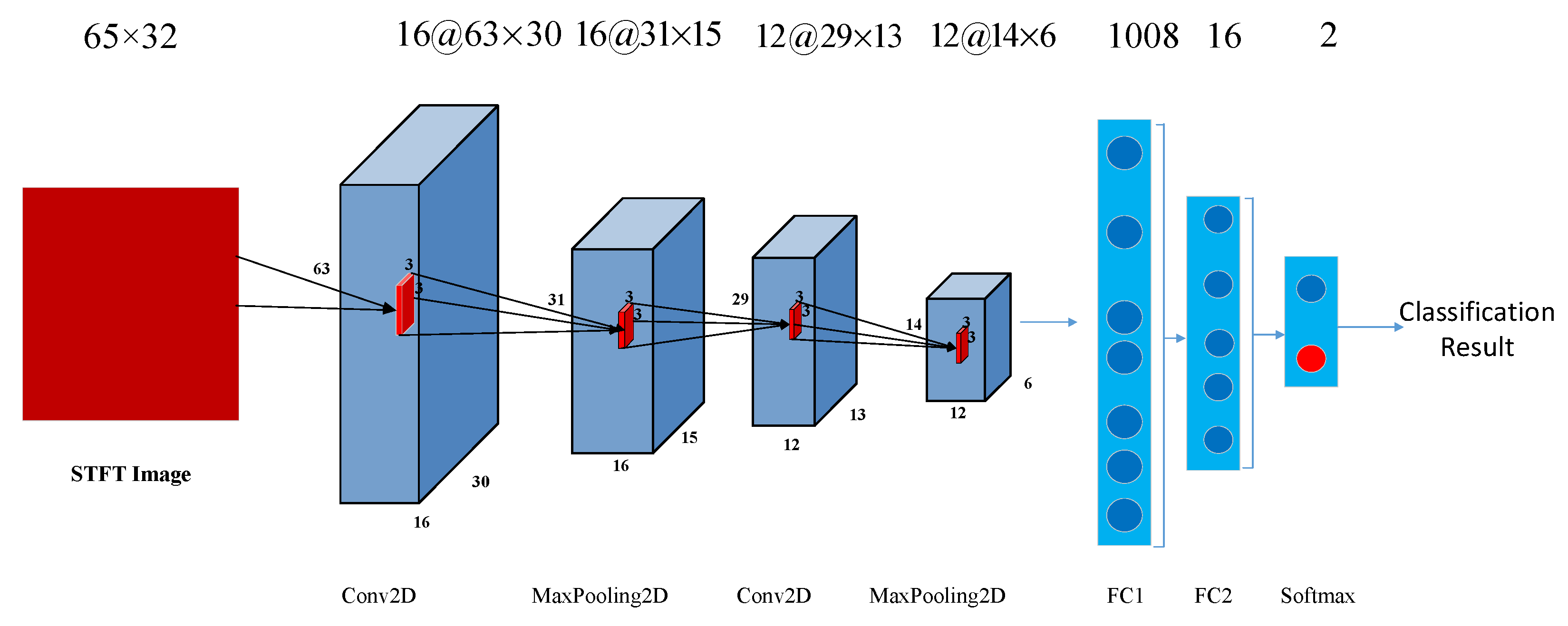
The architectures of different methods are depicted here. The number of convolutional layers plays a crucial role in detecting high-level concepts [36]. By comparing the proposed approaches, we aim to find an approach with better performance and the requirement of fewer computational resources. Considering that the echo signal is generated by a complex propagating process inside the minerals, we assume it has non-stationary characteristics, indicating that the frequency contents and time-domain characteristics of the signal change with time in the case of FC. Although the sediment is not rigorously homogeneous all around the survey area, the echo signal can be considered stationary when the acoustic signal goes through the non-ferromanganese crust (NonFC), like sediment, since the changes within the FC layers are much more relevant than those in the sediment’s characteristics. We focus on three baseline approaches, i.e., the features of STFT (short-term Fourier transform) with 2D-CNN, FFT (fast Fourier transform) with DNN, and the time-domain waveform with 1D-DNN.

3.2.1. STFT+2D-CNN

The feature of STFT is extracted from the secondary signal with an FFT length of 128, the Hanning window type, a window size of 128, and a hop length of 32, respectively. The feature size is 65 × 32, where 65 denotes the length of the vector of frequency amplitude and 32 denotes the number of frames. The STFT feature is fed to the CNN network with a simplified architecture, as shown in Figure 4. Aiming to realize the fast recognition function, we design the network architecture with a reduced computational burden. The number of training parameters is 18,078 for this network. The details are listed as follows:

• Stage 0: The input layer is an STFT image with a size of 65 × 32.
• Stage 1: The first stage consists of a convolutional layer of 16 filters with the rectangular shape of 3 × 3 and a stride of 1 × 1. We use a Rectified Linear Unit (ReLU) as the activation function and max pooling of 2 × 2 and a stride of 2 × 2.
• Stage 2: The second stage uses a convolutional layer of 12 filters with the rectangular shape of 3 × 3 and stride of 1 × 1. It is paddled with the method of valid paddling. We use a ReLU as the activation function. The max pooling of 2 × 2 and a stride of 2 × 2 is used. The dropout strategy with 0.5 is used in this layer.
• Stage 3: The stage contains the flatten layer with the number of hidden units of the first fully connected layer of 1008, followed by the connected layer with 16 hidden units and the dropout with 0.5. The binary output layer uses the cost function of softmax.
• Stage 4: This stage contains the flatten layer with 576 hidden units in the first fully connected layer, followed by the connected layer with 64 hidden units and the dropout with 0.5. The binary output layer uses the cost function of softmax.

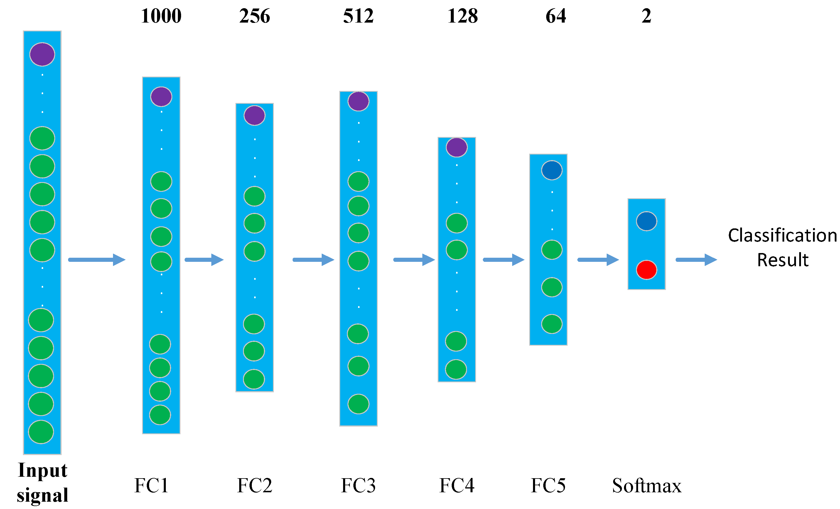
3.2.2. FFT+DNN

Considering the secondary signal has a length of 1000, we straightforwardly apply FFT to the waveform with the size of 1000. We take the amplitude vector in the frequency domain as the feature and insert it into the DNN network. Note that we do not use any concatenated features as the input of the model since we want to reduce the complexity to make real-time calculation possible. The number of training parameters is 461,890 for this network. As shown in Figure 5, the DNN model consists of an input layer and five hidden layers, and the number of neurons in each layer is set to be 1000, 256, 512, 128, and 64, respectively. We use ReLU as the activation function in all hidden layers. The dropout strategy with 0.5 is used in the first two hidden layers. The output layer takes softmax as the cost function.

3.2.3. Time-Domain Signal+1D-CNN

The network of 1D-CNN is similar to a regular neural network, but it takes a 1D signal waveform as the input of handcrafted features. Such input data are processed through several trainable convolutional layers to obtain a representative input form. The input signal given here is the preprocessed acoustic signal denoted as X. The convolutional structures can learn a set of parameters Θ and realize the prediction T, as shown in Equation (2):

$$T=F\left(X|\Theta \right)=f_L\left(...f_2\left(f_1\left(X|{\Theta }_1\right)|{\Theta }_2\right)|{\Theta }_L\right)$$

(2)

where L is the number of layers in the network.

We present a compact 1D CNN architecture with a reduced number of parameters, which reduces the computational burden to train such a network, as shown in Figure 6. The classifier has three convolutional layers interlaced with max-pooling layers and three fully connected layers. Considering that the valid duration of the preprocessed secondary signal is 2 μs with a sampling rate of 2 MHz, the model’s input size is 1000. As in the first convolutional layer, we design it with large receptive fields to obtain a more global view of the secondary signal since shorter filters cannot provide a general view of the spectral contents of the signal. After calculating all the parameters of the convolutional layers, we flatten the output of the last pooling layer and connect it to a fully connected layer. Since the amount of data for training is limited, we use a dropout of 0.5 for the two fully connected layers instead of deeper architectures to avoid significant over-fitting. The last fully connected layer has two neurons for binary classification. The ReLU activation function is used for all layers, except for the last fully connected layer with the activation function of softmax. Such a network can dispose of the extraction of complex handcraft features, and it is good enough to extract relevant low-level and high-level information from the secondary signal automatically. The number of training parameters is 87,346 for this network. The details of the simplified architecture are listed as follows:

• Stage 0: The input layer uses the time-domain signal with the size of 1000 as the input.
• Stage 1: The first stage consists of a convolutional layer of 16 filters with a rectangular shape of 64 and a stride of 2. We use a Rectified Linear Unit (ReLU) as the activation function and max pooling of 2 and a stride of 2.
• Stage 2: The second stage consists of a convolutional layer of 32 filters with a rectangular shape of 32 and a stride of 2. We use a ReLU as the activation function and max pooling of 2 and a stride of 2.
• Stage 3: This stage consists of a convolutional layer of 64 filters with a rectangular shape of 16 and a stride of 2. We use a ReLU as the activation function and max pooling of 2 and a stride of 2.
• Stage 4: This stage contains the flatten layer with 576 hidden units in the first fully connected layer, followed by the connected layer with 64 hidden units and dropout with 0.5. The binary output layer uses the cost function of softmax.

4. Experimental Configurations and Results

4.1. Experimental Configuration and Dataset Description

To fully evaluate the feasibility of the proposed method, the dataset is collected from two sea trials whose configurations are presented in Figure 7 with the setting parameters listed in

Table 1. The working parameters of PPPAAP19 for acquiring the dataset.

Parameter	Symbol	Value
Centroid frequency of the primary channel	$f_{0H}$	1 MHz
The bandwidth of the primary channel	$B{W}_H$	200 kHz
The sampling frequency of the primary channel	$f_{sH}$	5 MHz
The sampling frequency of the secondary channel	$f_{sL2}$	2 MHz
Lower/Higher cut-off frequency of BPF of the secondary channel	$f{l}_{L2}$$/f{h}_{L2}$	100 kHz/380 kHz
Lower/Higher cut-off frequency of BPF of the primary channel	$f{l}_{H2}/f{h}_{H2}$	900 kHz/1100 kHz

.

As shown in Figure 7a, the first acoustic dataset of the FC was collected from the experiments carried out on the China Ocean 55th voyage in the Western Pacific Ocean in Oct 2019. PPPAAPP19 was mounted on the mobile drilling rig. We employed the sit-on-bottom stationary measurements as the scheme of data acquirement. This way, the mobile drilling rig lands fixed at the mountain’s shoulder. PPPAAPP19 mounted on the rig was about 100 cm away from the seabed in the vertical direction, and data acquired at more than ten stations were recorded.

The second part of the acoustic dataset was acquired from the 2020 standardized sea trial in the South China Sea in December 2020. As shown in Figure 7b, PPPAAPP19 was mounted beneath the sample blanket of JIAOLONG HOV. The oceanauts drove the HOV at a relatively slow velocity, with PPPAAPP19 located approximately 10 m from the ground. Since our device could only record the data within 3 m using the configured parameters, information for certain heights is not available, as shown in Figure 8. Besides, the data acquired at the start of the transmitting time is also removed to avoid processing the signal with leakage energy caused by the transmitter.

We evaluate the performance of different models using the sea-trial dataset. The timestamp is recorded together with the acoustic data. As shown in Figure 9, the labeling process is based on the real-time visual observation from seafloor TV images simultaneously obtained during the sea trial. Figure 9a,b presents two different kinds of scenarios of the 2019 sea trial that contain FC and NonFC, while Figure 9c,d displays scenarios of the 2020 sea trial that contains NonFC from different perspectives.

The data acquired at more than 20 sites in a fixed mode in 2019 and one survey line in 2020 are used. Specifically, the acoustic data of FC and NonFC obtained in 2019 are simultaneously guaranteed by visual observation from seafloor TV images and pointwise sampled from core drilling, while the acoustic data of NonFC obtained in 2020 are guaranteed by oceanauts in real-time. As shown in Figure 10, different samples corresponding to the acoustic data are presented. Based on this information, we label the data for the supervised classification.

The augmented method increases noise from the SNR from 1 dB to 6 dB with the step of 1 dB. After augmentation, the total number of records is 50,888, whereby that of the ferromanganese crust (FC) is 33,920 and that of the Non-Ferromanganese Crust (NonFC) is 16,968. As shown in

Table 2. The number of FC/NonFC for training/validation and test processing.

Original	# FC	# NonFC	# Total	Percent
Train/	18,120	9544	27,664	75% (Train/val = 3:1)
Val	6040	3182	9222
Test	9760	4242	14,002	25%
Total	33,920	16,968	50,888	100%

“#”denotes “the number of”.

, 75% of the data are used as the training/validation set, and 25% are used as the test set. Among them, 75% of the training/validation set is used for training, and 25% is used for validation. The dataset partitioning of the training/validation set and the test set is strictly independent to guarantee no data leakage. It can be seen that the number of FC is about twice that of NonFC.

Nine of the waveforms of FC, colored green, and Nine of NonFC, colored red, are presented in Figure 11. We can see that several waveforms of NonFC have similar trends, as do those of FC. For example, the waveforms of NonFC #47, #143, #226, #351, and #485 have a similar structure since the last peaks appear at around the 750th point. Moreover, the waveforms of FC #481 and #905 also have a similar structure, since the narrow peaks appear at the very beginning of the upper surface and their energies quickly attenuate. A possible reason for this is that the detected targets may have similar acoustic characteristics, such as acoustic impedance and inner structure. However, there are some differences between intra-class data and some similarities for inter-class data, such as the waveforms of NonFC #90 and #351 and the waveforms of FC #581, #601, and #1641. We can understand such phenomena according to the pictures of the obtained samples, considering that the acoustic impedance and inner structure could vary, as shown in Figure 10. It is worth noting that the data are acquired with the same configuration, i.e., the BPF of the secondary channel of 100 kHz–380 kHz and the BPF of the primary channel of 900 kHz–1100 kHz.

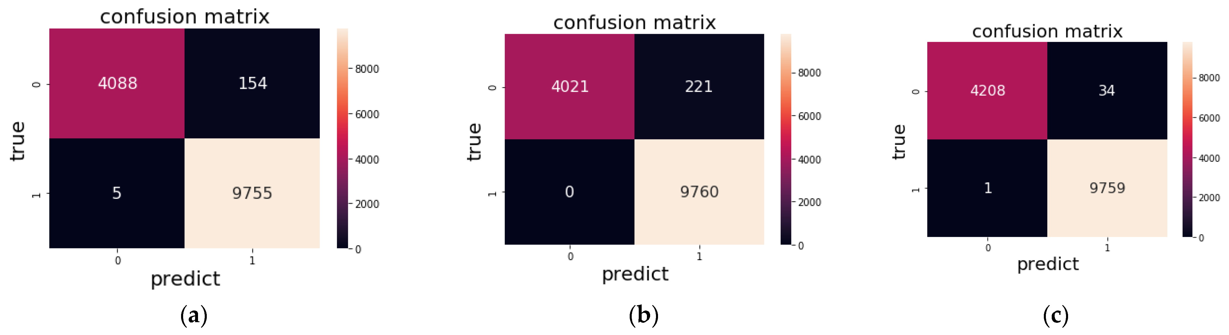
4.2. Result and Analysis

We use a computer with four GPUs of Nvidia GeForce RTX 2080Ti and Core i7-6900K CPU for training and testing. The deep learning framework of the model is implemented using Keras 2.2.4 with TensorFlow 1.12.0 as a backend. When training the model, the batch size and the maximum number of epochs are 64 and 100. We accelerate the training process with the early stopping strategy used to stop training if the validation loss is reduced by more than 0.00005 in 10 successive epochs. Besides, the adaptable learning rate strategy is adopted, where the initial value is 0.001 and the value is 60% of the former value every ten epochs. Note that we avoid overfitting by designing an adaptable learning rate.

The detailed results of the classification system for precision, recall, f1-score, and computational burden is given in

Table 3. Performance of different methods.

Method	Type	Precision	Recall	F1-Score	Support
STFT+2D-CNN (18,078)	FC	0.985	0.999	0.992	9760
	NonFC	0.998	0.966	0.982	4242
	weighted avg	0.989	0.989	0.989	14,002
		Precision	Recall	F1-Score	Support
FFT+DNN (461,890)	FC	0.978	1.000	0.989	9760
	NonFC	1.000	0.948	0.973	4242
	weighted avg	0.984	0.984	0.984	14,002
		Precision	Recall	F1-Score	Support
Time-domain + 1D-CNN (87,346)	FC	0.997	0.999	0.998	9760
	NonFC	0.999	0.992	0.996	4242
	weighted avg	0.998	0.998	0.997	14,002

. It is clear that the recognition rate of each class is higher than 0.90, and the weighted average precision, recall, or f1-score is higher than 0.98, where the support denotes the number of each test class. It is worth noting that parameters such as the number of filters, filter size, and the number of layers, and hyperparameters for training such as the batch size, the initial learning rate, and the patience in early stopping, are optimal choices according to the training and validation process in the experiment.

To better understand the performance of different methods, we present the confusion matrices of different methods, as shown in Figure 12. From the accuracy aspect, time-domain +1D-CNN can achieve the best performance, while STFT+2D-CNN is slightly worse. However, we can see that all these methods only misclassified several records, which do not have an apparent statistical difference in the aspect of accuracy. In other words, we can obtain high accuracy of the binary classification without a complex design of the deep learning networks. In contrast, from the perspective of computational burden, we can conclude that STFT+2D-CNN is assumed to be the most suitable network for real-time realization, while FFT+DNN is the worst network for binary classification. It is apparent that Time-domain+1D-CNN has the same order of the number of training parameters as STFT+2D-CNN. Nevertheless, if taking the computational cost of preprocessing into consideration, Time-domain+1D-CNN has an advantage over STFT+2D-CNN since it avoids the extra computation of STFT. In summary, Time-domain +1D-CNN is suitable for real-time realization with a high recognition rate and small computational burden.

5. Conclusions

We proposed a preprocessing method and data augment strategy to form the 2019 and 2020 sea trials dataset. The performances of several baseline approaches, i.e., STFT+2D-CNN, FFT+DNN, and Time-domain signal+1D-CNN, were assessed on the sea-trial dataset, and the experimental results showed that they all achieved excellent recognition accuracy for binary classification. However, considering the real-time processing requirement, we found that the end-to-end approach for binary classification based on 1D-CNN had a comprehensive advantage since it can directly receive the preprocessed acoustic signal as input to the classifier. Therefore, we have validated the possibility of binary classification for recognizing ferromanganese crust in an acoustic manner alone with the data obtained with a well-designed Parametric Acoustic Probe named PPPAAP19 and a deep learning-based algorithm. The proposed method provided good technical support for the future design of sonar systems. As for the performance of nodules in different concentrations on the seabed, this remains a focus for future research work.

References

1. Hein, J.R.; Koschinsky, A.; Bau, M.; Manheim, F.T.; Kang, J.; Roberts, L. Cobalt-rich ferromanganese crusts in the Pacific. Handb. Mar. Miner. Depos. 2000, 18, 239–273. [Google Scholar]
2. Clark, M.R.; Heydon, R.; Hein, J.R.; Petersen, S.; Rowden, A.; Smith, S.; Baker, E.; Beaudoin, Y. Deep Sea Minerals: Cobalt-Rich Ferromanganese Crusts, A Physical, Biological, Environmental, and Review; Baker, E., Beaudoin, Y., Eds.; Secretariat of the Pacific Community: Noumea, France, 2013. [Google Scholar]
3. Usui, A.; Nishi, K.; Sato, H.; Nakasato, Y.; Thornton, B.; Kashiwabara, T.; Tokumaru, A.; Sakaguchi, A.; Yamaoka, K.; Kato, S.; et al. Continuous growth of hydrogenetic ferromanganese crusts since 17 Myr ago on Takuyo-Daigo Seamount, NW Pacific, at water depths of 800–5500 m. Ore Geol. Rev. 2017, 87, 71–87. [Google Scholar] [CrossRef] [Green Version]
4. Usui, A.; Graham, I.J.; Ditchburn, R.G.; Zondervan, A.; Shibasaki, H.; Hishida, H. Growth history and formation environments of ferromanganese deposits on the Philippine Sea Plate, northwest Pacific Ocean. Island Arc 2007, 16, 420–430. [Google Scholar] [CrossRef]
5. Yang, Y.; He, G.; Ma, J.; Yu, Z.; Yao, H.; Deng, X.; Liu, F.; Wei, Z. Acoustic quantitative analysis of ferromanganese nodules and cobalt-rich crusts distribution areas using EM122 multibeam backscatter data from deep-sea basin to seamount in Western Pacific Ocean. Deep. Sea Res. Part I Oceanogr. Res. Pap. 2020, 161, 103281. [Google Scholar] [CrossRef]
6. Hong, F.; Feng, H.; Huang, M.; Wang, B.; Xia, J. China’s First Demonstration of Cobalt-rich Manganese Crust Thickness Measurement in the Western Pacific with a Parametric Acoustic Probe. Sensors 2019, 19, 4300. [Google Scholar] [CrossRef] [Green Version]
7. Du, D.; Ren, X.; Yan, S.; Shi, X.; Liu, Y.; He, G. An integrated method for the quantitative evaluation of mineral resources of cobalt-rich crusts on seamounts. Ore Geol. Rev. 2017, 84, 174–184. [Google Scholar] [CrossRef]
8. Neettiyath, U.; Thornton, B.; Sangekar, M.; Nishida, Y.; Ishii, K.; Bodenmann, A.; Sato, T.; Ura, T.; Asada, A. Deep-Sea Robotic Survey and Data Processing Methods for Regional-Scale Estimation of Manganese Crust Distribution. IEEE J. Ocean. Eng. 2020, 46, 102–114. [Google Scholar] [CrossRef]
9. Neto, A.A.; Da Costa, V.A.; Porto, C.P.F.M.; Garrido, T.C.V.; Hermand, J.-P. Relationship between geoacoustic properties and chemical content of submarine polymetallic crusts from offshore Brazil. Mar. Georesources Geotechnol. 2019, 38, 437–449. [Google Scholar] [CrossRef]
10. Anderson, J.T.; Holliday, V.; Kloser, R.; Reid, D.; Simard, Y. Acoustic seabed classification of marine physical and biological landscapes. ICES Coop. Res. Rep. 2007, 286. Available online: https://www.researchgate.net/profile/Andrzej-Orlowski/publication/263887329_Acoustic_seabed_classification_of_marine_physical_and_biological_landscapes/links/55c3579808aeca747d5e1b39/Acoustic-seabed-classification-of-marine-physical-and-biological-landscapes.pdf (accessed on 6 October 2021).
11. Michaels, W.L. Review of acoustic seabed classification systems. In Acoustic Seabed Classification of Marine Physical and Biological Landscapes; Anderson, J.T., Holliday, D.V., Kloser, R., Reid, D.G., Simard, Y., Eds.; ICES: Copenhagen, Denmark, 2007; Volume 286, pp. 94–115. Available online: https://www.researchgate.net/publication/280741003 (accessed on 6 October 2021).
12. Kloser, R. Seabed backscatter, data collection and quality overview. In Acoustic Seabed Classification of Marine Physical and Biological Landscapes; ICES Cooperative Research Report; Anderson, J.T., Ed.; ICES Cooperative: Copenhagen, Denmark, 2007; Volume 286, pp. 45–60. Available online: https://www.vliz.be/en/imis?module=ref&refid=114460 (accessed on 6 October 2021).
13. Machida, S.; Fujinaga, K.; Ishii, T.; Nakamura, K.; Hirano, N.; Kato, Y. Geology and geochemistry of ferromanganese nodules in the Japanese Exclusive Economic Zone around Minamitorishima Island. Geochem. J. 2016, 50, 539–555. [Google Scholar] [CrossRef] [Green Version]
14. Usui, A.; Okamoto, N. Geophysical and geological exploration of cobalt-rich ferromanganese crusts: An attempt of small-scale mapping on a Micronesian seamount. Mar. Georesour. Geotechnol. 2010, 28, 192–206. [Google Scholar] [CrossRef]
15. Nakamura, K.; Machida, S.; Okino, K.; Masaki, Y.; Iijima, K.; Suzuki, K.; Kato, Y. Acoustic characterization of pelagic sediments using sub-bottom profiler data: Implications for the distribution of REY-rich mud in the Minamitorishima EEZ, western Pacific. Geochem. J. 2016, 50, 605–619. [Google Scholar] [CrossRef] [Green Version]
16. Machida, S.; Sato, T.; Yasukawa, K.; Masaki, Y.; Iijima, K.; Suzuki, K.; Kato, Y. Visualisation method for the broad distribution of seafloor ferromanganese deposits. Mar. Georesour. Geotechnol. 2021, 39, 267–279. [Google Scholar] [CrossRef] [Green Version]
17. Berthold, T.; Leichter, A.; Rosenhahn, B.; Berkhahn, V.; Valerius, J. Seabed sediment classification of side-scan sonar data using convolutional neural networks. In Proceedings of the 2017 IEEE Symposium Series on Computational Intelligence (SSCI) 2017, Honolulu, HI, USA, 27 November–1 December 2017. [Google Scholar]
18. Ma, J.; Li, H.; Zhu, J.; Chen, B. Sound Velocity Estimation of Seabed Sediment Based on Parametric Array Sonar. Math. Probl. Eng. 2020, 2020, 9810215. [Google Scholar] [CrossRef]
19. Weydert, M.M.P. Measurements of the acoustic backscatter of manganese nodules. J. Acoust. Soc. Am. 1985, 78, 2115–2121. [Google Scholar] [CrossRef]
20. Weydert, M.M.P. Measurements of the acoustic backscatter of selected areas of the deep seafloor and some implications for the assessment of manganese nodule resources. J. Acoust. Soc. Am. 1990, 88, 350–366. [Google Scholar] [CrossRef]
21. Hein, J.R.; Mizell, K.; Koschinsky, A.; Conrad, T.A. Deep-ocean mineral deposits as a source of critical metals for high-and green-technology applications: Comparison with land-based resources. Ore Geol. Rev. 2013, 51, 1–14. [Google Scholar] [CrossRef]
22. Lusty, P.A.J.; Murton, B.J. Deep-ocean mineral deposits: Metal resources and windows into earth processes. Elements 2018, 14, 301–306. [Google Scholar] [CrossRef] [Green Version]
23. Moustier, C. Inference of manganese nodule coverage from Sea Beam acoustic backscattering data. Geophysics 1985, 50, 989–1001. [Google Scholar] [CrossRef]
24. Chakraborty, B.; Kodagali, V.; Baracho, J. Sea-floor classification using multibeam echo-sounding angular backscatter data: A real-time approach employing hybrid neural network architecture. IEEE J. Ocean. Eng. 2003, 28, 121–128. [Google Scholar] [CrossRef]
25. Weydert, M. Design of a system to assess manganese nodule resources acoustically. Ultrasonics 1991, 29, 150–158. [Google Scholar] [CrossRef]
26. Choening, T.; Jones, D.O.B.; Greinert, J. Compact-morphology-based polymetallic nodule delineation. Sci. Rep. 2017, 7, 13338–13349. [Google Scholar] [CrossRef] [PubMed]
27. Hari, V.N.; Kalyan, B.; Chitre, M.; Ganesan, V. Spatial modeling of deep-sea ferromanganese nodules with limited data using neural networks. IEEE J. Ocean. Eng. 2017, 43, 997–1014. [Google Scholar] [CrossRef]
28. Wang, B.; Hong, F.; Feng, H.; Huang, M.; Xia, J.; Liu, C. Evaluation of the recognition of Cobalt-Rich Manganese Crusts based on Deep Learning Networks with physical phantoms. In Global Oceans 2020, Singapore-U.S. Gulf Coast; IEEE: New York, NY, USA, 2020; pp. 1–5. [Google Scholar]
29. Thornton, B.; Asada, A.; Bodenmann, A.; Sangekar, M.; Ura, T. Instruments and methods for acoustic and visual survey of manganese crusts. IEEE J. Ocean. Eng. 2012, 38, 186–203. [Google Scholar] [CrossRef]
30. Neettiyath, U.; Sato, T.; Sangekar, M.; Bodenmann, A.; Thornton, B.; Ura, T.; Asada, A. identification of manganese crusts in 3D visual reconstructions to filter geo-registered acoustic sub-surface measurements. In OCEANS 2015-MTS/IEEE Washington; IEEE: New York, NY, USA, 2015; pp. 1–6. [Google Scholar]
31. Hong, F.; Liu, C.; Guo, L.; Chen, F.; Feng, H. Underwater Acoustic Target Recognition with a Residual Network and the Optimized Feature Extraction Method. Appl. Sci. 2021, 11, 1442. [Google Scholar] [CrossRef]
32. Ji, X.; Yang, B.; Tang, Q. Seabed sediment classification using multibeam backscatter data based on the selecting optimal random forest model. Appl. Acoust. 2020, 167, 107387. [Google Scholar] [CrossRef]
33. Neilsen, T.B.; Escobar-Amado, C.D.; Acree, M.C.; Hodgkiss, W.S.; van Komen, D.F.; Knobles, D.P.; Badiey, M.; Castro-Correa, J. Learning location and seabed type from a moving mid-frequency source. J. Acoust. Soc. Am. 2021, 149, 692. [Google Scholar] [CrossRef]
34. Miller, K.A.; Thompson, K.F.; Johnston, P.; Santillo, D. An overview of seabed mining including the current state of development, environmental impacts, and knowledge gaps. Front. Mar. Sci. 2018, 4, 418. [Google Scholar] [CrossRef]
35. Zhua, Z.; Cui, X.; Zhang, K.; Ai, B.; Shi, B.; Yang, F. DNN-based seabed classification using differently weighted MBES multi features. Mar. Geol. 2021, 438, 106519. [Google Scholar] [CrossRef]
36. Abdoli, S.; Cardinal, P.; Koerich, A. End-to-end environmental sound classification using a 1D convolutional neural network. Expert Syst. Appl. 2019, 136, 252–263. [Google Scholar] [CrossRef] [Green Version]
Figure 1. The photo of Programmable Phased Parametric Array Acoustic Probe 2019 (PPPAAP19): (a) Front view of PPPAAP19; (b) the designed array located at the bottom of PPPAAP19 with the receiving transducer marked with red and the other 18 transmitting transducers around it.
Minerals 12 00249 g001
Figure 2. System description of PPPAAP19 with the host computer.
Minerals 12 00249 g002
Figure 3. Binary classification with different approaches.
Minerals 12 00249 g003
Figure 4. Binary classification with the approach of STFT+2D-CNN.
Minerals 12 00249 g004
Figure 5. Binary classification with the approach of FFT+DNN.
Minerals 12 00249 g005
Figure 6. Binary classification with the approach of time-domain signal+1D-CNN.
Minerals 12 00249 g006
Figure 7. Experimental configurations to acquire the echo data: (a) PPPAAPP19 mounted on the mobile drilling rig in 2019; (b) PPPAAPP19 mounted on JIAOLONG HOV in 2020. The development of the device has a label that indicates it is supported by National key R&D Program.
Minerals 12 00249 g007aMinerals 12 00249 g007b
Figure 8. Estimated height away from the seabed in 2020 standardized sea trial.
Minerals 12 00249 g008
Figure 9. Pictures of (a,b) two different kinds of scenarios of the 2019 sea trial that contain FC and NonFC and (c,d) scenarios of the 2020 sea trial that contains NonFC from different perspectives.
Minerals 12 00249 g009
Figure 10. Samples of the survey area. (a) Several samples of FC and NonFC. (b) Other samples of FC and NonFC and the card indicates that they were obtained by Guangzhou Marine Geological Survey.
Minerals 12 00249 g010
Figure 11. Some of the waveforms of FC, colored green, and those of NonFC, colored red.
Minerals 12 00249 g011
Figure 12. Confusion matrices of different methods. (a) STFT+2D-CNN; (b) FFT+DNN; (c) Time-domain signal+1D-CNN.
Minerals 12 00249 g012