Modeling Interfacial Tension of N₂/CO₂ Mixture + n-Alkanes with Machine Learning Methods: Application to EOR in Conventional and Unconventional Reservoirs by Flue Gas Injection

Abstract

The combustion of fossil fuels from the input of oil refineries, power plants, and the venting or flaring of produced gases in oil fields leads to greenhouse gas emissions. Economic usage of greenhouse and flue gases in conventional and unconventional reservoirs would not only enhance the oil and gas recovery but also offers CO₂ sequestration. In this regard, the accurate estimation of the interfacial tension (IFT) between the injected gases and the crude oils is crucial for the successful execution of injection scenarios in enhanced oil recovery (EOR) operations. In this paper, the IFT between a CO₂/N₂ mixture and n-alkanes at different pressures and temperatures is investigated by utilizing machine learning (ML) methods. To this end, a data set containing 268 IFT data was gathered from the literature. Pressure, temperature, the carbon number of n-alkanes, and the mole fraction of N₂ were selected as the input parameters. Then, six well-known ML methods (radial basis function (RBF), the adaptive neuro-fuzzy inference system (ANFIS), the least square support vector machine (LSSVM), random forest (RF), multilayer perceptron (MLP), and extremely randomized tree (extra-tree)) were used along with four optimization methods (colliding bodies optimization (CBO), particle swarm optimization (PSO), the Levenberg–Marquardt (LM) algorithm, and coupled simulated annealing (CSA)) to model the IFT of the CO₂/N₂ mixture and n-alkanes. The RBF model predicted all the IFT values with exceptional precision with an average absolute relative error of 0.77%, and also outperformed all other models in this paper and available in the literature. Furthermore, it was found that the pressure and the carbon number of n-alkanes would show the highest influence on the IFT of the CO₂/N₂ and n-alkanes, based on sensitivity analysis. Finally, the utilized IFT database and the area of the RBF model applicability were investigated via the leverage method.

1. Introduction

To produce crude oil from a reservoir, three methods are available: primary, secondary, and tertiary or enhanced oil recovery (EOR). EOR is a way to produce reducible oil in the reservoir which is defined as a set of techniques and processes that increases the amount of oil recovery by employing energy and the injection of materials [1,2,3]. Improved oil recovery (IOR) and EOR are used to increase the recovery factor of remained oil in reservoirs. The main objective of EOR focuses on the immobile oil that is trapped because of the viscous forces and/or capillary. Thus, the reduction of the residual oil, improving the displacement efficiency (microscopic) as compared to ordinary water flooding, or increasing the volumetric sweep efficiency (macroscopic) are the main objectives of all EOR techniques. Herein, the reduction of interfacial tension (IFT) can help to increase EOR by removing the trapped oil. Moreover, it can increase the two-phase miscibility and improve oil recovery [2,3]. EOR is divided into several methods, such as gas injection, chemical EOR, thermal EOR, and other new technologies. In gas injection, different gases are injected into the reservoir, which consists of flue gases, hydrocarbons, air, N₂, CO₂, and a mixture of gases. The ability of CO₂ to interact with the reservoir fluid makes it attractive to use for this specific purpose. Another advantage of CO₂ injection is storing it underground, as CO₂ is a greenhouse gas. The cyclic injection ability and accessibility of N₂ in the air, as well as its low cost, makes it an attractive option for EOR operations. Hence, the mixture of N₂ and CO₂ could have the advantages of both gases when they are being used separately [4]. Flue gas, as the main emissions of industrial operations, contains mainly CO₂ and N₂ along with CO, SO₂, and water vapor. Studies have shown that non-CO₂ and CO₂ gases emitted as flue gas during fuel combustion, cement clinker production, etc., can be sequestered in depleted or mature hydrocarbon reservoirs, coal seams, and saline aquifers [5]. Moreover, raw flue gas injection into oil reservoirs can benefit us in two ways, both the incremental oil recovery due to special properties of CO₂/N₂ gases and the sequestration of these greenhouse gases into the reservoirs if the structural seals for trapping them is confirmed [6,7].

In relation to enhanced shale oil/gas recovery techniques by gas injection, depending on the fluids with special features considering the reservoir circumstances, injected gas can be CO₂, N₂, flue gas, and produced gases [8]. However, it has been shown that injecting gas into shale oil reservoirs, regardless of the type of injected gas, can recover significant oil, even if the injected gas is not completely miscible with the reservoir oil [9]. During oil recovery, significant produced gas associated with oil production is released into the air or flared that is hazardous to the environment and is considered a waste of energy. These produced gases can be utilized for recycled gas EOR in order to compensate for the oil production decline and reduce gas release or flaring [8,10]. CO₂ injection in shale reservoirs can enhance oil or natural gas recovery via multicontact miscible displacement, maintaining pressure, the desorption of methane, and molecular diffusion along with permanent sequestration within the small pores in an adsorbed state [8,11,12,13,14]. Additionally, due to the high minimum miscibility pressure, an immiscible displacement approach can help displace the oil by utilizing the injection of N₂ as an economical and environmentally friendly alternative. Furthermore, flue gases have been successfully injected in unconventional reservoirs, including gas hydrate and coalbed methane, and are regarded as a potential injection gas resource for shale reservoirs [8]. Gas hydrates, ice-like crystalline solids consisting of water and gas molecules, mainly methane that are trapped in permafrost regions and subsea sediments [15,16], can be decomposed if pressure and temperature are outside their hydrate stability zone, or the chemical equilibrium between the hydrate phase and the adjacent environment is disturbed [16]. Researchers have illustrated that flue gas injection into gas hydrate reservoirs, as a type of unconventional reservoir, is associated with the fast dissociation of the methane hydrate by shifting the methane hydrate stability zone. This affordable method has been considered a promising one that improves the feasibility of methane recovery from gas hydrate reservoirs and CO₂ sequestration in geological formations [15].

IFT plays a crucial role in all EOR processes, especially gas injection. IFT is strongly affected by the composition of the two phases, pressure, and temperature. This property can be measured by experimental techniques, such as pendent and springing drop methods, that are expensive and time-consuming. Thus, calculating the IFT via modeling is an alternative method that should be considered. The Parachor model, thermodynamic correlations, gradient theory, and corresponding state theory are among the most famous models for predicting the IFT, while Parachor has been used extensively in the petroleum industry. Nevertheless, this model also needs us to apply an equation of state (EOS), as well as flash calculations, which compromises its accuracy [17].

To overcome the above challenge, artificial intelligence (AI) methods that have been utilized in the petroleum industry for various purposes, including IFT estimation, can be an alternative solution. AI is an instinctive mechanism that performs different tasks such as observing, learning, and reasoning [18]. AI is an interdisciplinary science with multiple approaches. Some of the most important successful applications of AI are “classification”, “forecasting”, “control systems”, and “optimization and decision making” [19]. Machine learning (ML) is a branch of AI and computer science which focuses on the usage of data and algorithms to imitate the way that humans learn, thus gradually improving its accuracy. ML focuses on the computer program development that can change when exposed to new data. In addition, deep learning (DL) is a class of ML techniques that utilizes multilayered neural networks [20,21]. In the following section, some of the recent models in this area are briefly reviewed. It should be noted, as the dominant fluids that exist in the reservoir are oil and water, that the majority of ML models were developed to predict the IFT in oil−brine [22,23], water−hydrocarbon [24,25], brine−hydrocarbon [26,27,28], and CO₂−brine [29,30,31,32] systems. Ahmadi and Mahmoudi [33] predicted the gas–oil IFT with least squares support vector machines (LSSVM) as a well-known ML method. For the whole data set, their model yielded the coefficient of determination (R²) of 0.998. One small drawback of this model is the low data range. Ayatollahi et al. [34] modeled the IFT and minimum miscibility pressure (MMP) between normal-alkane and the injecting gas (CO₂) by LSSVM. The developed model could predict the IFT values with an average absolute percent relative error (AAPRE) of 4.7%. Moreover, pressure had the greatest influence on the IFT among the inputs. Hemmati-Sarapardeh and Mohagheghian [35] implemented the group method of data handling (GMDH) for modeling the IFT and MMP in paraffin–N₂ systems. GMDH is a family of inductive algorithms for computer-based mathematical modeling of multiparametric datasets. This model estimates the data satisfactorily, with AAPRE values of 3.91% and 3.81% in the testing and training subsets, respectively. Based on the relevancy factor, pressure plays an important role in the IFT modeling of paraffin–N₂ systems. Shang et al. [36] studied the IFT of the CO₂/N₂ mixture + paraffin. They also proposed an empirical correlation for predictions of IFT data with a mean absolute relative error of 4.47%. Ameli et al. [1] used three famous ML methods, including the radial basis function (RBF) and multilayer perceptron (MLP) neural networks along with LSSVM, for estimating the IFT in N₂/n-alkane systems. The MLP trained with the Levenberg–Marquardt algorithm obtained the most accurate predictions, with an AAPRE of 1.38%. The advantages of this research are the low error, acceptable data range, and a reliable database with just a few outliers. Zhang et al. [37] utilized the extreme gradient boosting tree method as a supervised branch of ML for estimating the IFT of gas/n-alkane. The model’s results (root mean square error (RMSE) and R²) were 0.15 mN/m and 0.99 for the train subset and 0.57 mN/m and 0.99 for the testing subset. They concluded that pressure and n-alkane’s molecular weight have the highest effect on the IFT. Rahul Gajbhiye [4] experimentally investigated the impact of CO₂/N₂ mixture composition on the IFT of crude oil and gas systems. The outcomes of this study confirmed that the IFT of the crude oil and CO₂/N₂ gas mixture increased with an increase in the fraction of N₂ and decreased with an increase in the fraction of CO₂. Mirzaie and Tatar [38] utilized EOS and gene expression programming (GEP) to model the IFT in binary mixtures of N₂, CH₄, and CO₂–alkanes. GEP is an evolutionary algorithm that creates computer programs or models that can be used to develop mathematical correlations. Conversely, the EOS model failed to present the IFT results for some experimental observations. For the GEP model in CH₄, CO₂, and N₂–alkanes systems, the R² values were 0.92, 0.94, and 0.91, respectively. Rezaei et al. [17] compared soft computing techniques, empirical correlations, and the Parachor model in estimating the IFT of CO₂–paraffin systems and concluded that the RBF neural network optimized by the imperialist competitive algorithm has the most reliable prediction. According to our information and the literature review, there is not any AI model to predict the IFT relationship between the CO₂/N₂ mixture and n-alkanes (as the main constitutes of crude oil) so far. Hence, this work attempts to fulfill this gap and present accurate ML models for predicting the IFT of the CO₂/N₂ mixture and n-alkanes. To do so, the IFT of the CO₂/N₂ mixture and n-alkanes is modeled by utilizing six well-known ML methods along with four optimization methods and a database containing 268 IFT data at varying pressures and temperatures. Moreover, sensitivity analysis is performed to determine the influence of the input parameters on the IFT of n-alkanes and the CO₂/N₂ mixture. Eventually, the applicability of the best-developed model is examined by the leverage approach.

2. Data Collection

A dataset with a broad range of data containing 268 IFT data points is collected from the literature [36,39]. The IFT database utilized for modeling in this research is presented in Table S1. Pressure, temperature, the carbon number of n-alkanes, and the mole fraction of N₂ are selected as input variables to the model. The output of the model is the IFT of the N₂/CO₂ mixture + n-alkanes. Statistical data of each column of inputs and target data are also presented in

Table 1. Statistical data of each column of inputs and target data.

IFT (mN/m)	N2 (Mole Fraction)	Carbon Number	Temperature (°C)	Pressure (MPa)
1.75	0.25	5	30	0.1	Minimum
22.93	1	17	120	40.16	Maximum
10.33	0.25	13	40	0.1	Mode
11.11	0.25	11	60	7.8	Median
11.71	0.43	11.28	67.99	8.78	Mean
0.3833	1.1845	0.0067	0.4725	1.7978	Skewness
−0.5802	−0.6015	−1.0395	−1.0451	4.6985	Kurtosis

. This statistical information demonstrated that the variation and distribution of model input parameters are broad enough to be able to develop a model for estimating the IFT of the N₂/CO₂ mixture + n-alkanes.

3. Methodology

AI has several great branches, known as neural networks, ML, and expert systems. ML is a subset of AI and provides computers the ability to learn without being explicitly programmed. As a simple definition, ML is any type of computer program that can “learn” by itself and where humans have no role during learning. DL is defined as a form of ML that can apply either supervised, unsupervised algorithms, or both. Artificial neural networks (ANNs) are a subset of ML and are at the heart of DL algorithms [40]. In the last decades, a wide range of engineering problems has been solved by inductive ML algorithms [23,24,41]. ANNs are suited towards tasks that include fuzzy or incomplete information, complex and ill-defined problems, and incomplete data sets, where they are usually decided on a visional basis. ANNs can be trained from real examples and are able to address nonlinear problems. Furthermore, they display robustness and fault tolerance. Classification, forecasting, and control systems are some of the most important successful applications of ANNs [19].

A general flowchart for the implemented algorithms for the development of the IFT models that were used in this work is shown in Figure 1.

3.1. Model Development

3.1.1. Multilayer Perceptron

MLP is an algorithm that is classified as a feed-forward ANN with several layers. The term MLP is usually applied for feed-forward ANNs and networks composed of several layers of perceptrons, loosely and strictly, respectively (with threshold activation). The first and the latest layer are contacted with inputs and outputs data (or targets) [42]. MLP includes at least three layers: input, hidden, and output layers. Each layer involves several nodes that are considered as neurons (their number depends on the number of input and output parameters) that utilize a nonlinear activation function only for the hidden layers and the output layer [43]. Training an ANN can be done by supervised, unsupervised, and semisupervised learning. MLP uses a supervised learning technique dubbed backpropagation. MLP is a good algorithm for data that is not linearly separable [1].

An MLP has some activation functions that map the weighted inputs to the output of each neuron. Commonly utilized activation functions are sigmoids, which are formulated below:

$$\mathrm{y} \left(\mathrm{vi}\right) = \tan \mathrm{h} \left(\mathrm{vi}\right)\mathrm{andy}\left(\mathrm{vi}\right) ={\left(1+{\mathrm{e}}^{-\mathrm{vi}}\right)}^{-1}$$

(1)

The hyperbolic tangent ranges from −1 to 1, while the logistic function with similar shape ranges from 0 to 1.

In the perceptron, when connection weights change, learning occurs after each piece of data is processed on the basis of error amount in the predicted values compared to the experimental data. In the present work, tansig (tangent hyperbolic) in the hidden layers and pureline (linear function) in the output layer were utilized as transfer functions. These transfer functions are the followings [1]:

Tansig transfer functions

$$f\left(x\right)=\frac{2}{1+exp \left(-2x\right)}-1$$

(2)

Pureline transfer functions

$$f\left(x\right)=x$$

(3)

Logsig transfer functions

$$Logsig \left(n\right) =1 / \left(1+exp \left(-n\right)\right)$$

(4)

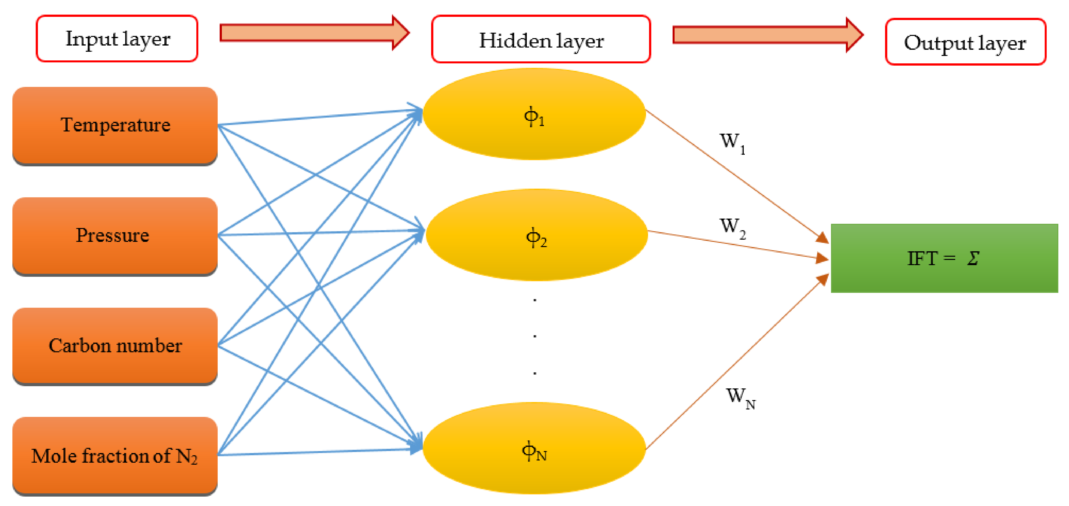
3.1.2. Radial Basis Function Neural Network

For mathematical modeling and physics problems, an RBF network [44] as a kind of ANN can be an attractive choice. The activation functions of RBF are radial basis functions [1]. To calculate the output, the linear combination of the RBFs of the inputs and neuron parameters are utilized. RBF networks usually include three layers: a linear output layer, an input layer, and a hidden layer with a nonlinear RBF activation function. A schematic of an RBF network is depicted in Figure 2. The input can be modeled as a vector of real numbers x ϵ Rⁿ, and the result of the network is a scalar function of the input vector, φ: R → Rⁿ, and is obtained by:

$$\phi \left(x\right)={{\displaystyle \sum }}_{i=1}^n{a}_i\rho \left(\left|\left|x-c_i\right|\right|\right)$$

(5)

where C_i shows the center vector for neuron i, a_i stands for the weight of the neuron in the linear output neuron, and N denotes the count of neurons in the hidden layer. Basically, all inputs are connected to every hidden neuron. The rule is usually taken to be the Euclidean distance (although the Mahalanobis distance performs better, generally) and RBF is established on the Gaussian method. The Gaussian radial basis function is as follows:

$$\rho \left(\left|\left|x-c_i\right|\right|\right) =\exp \left[-\beta {\left|\left|x-c_i\right|\right|}^2\right]$$

(6)

Gaussian basis functions search the center vector in the sense that:

$$\underset{\left|\left|x\right|\right| \to \infty }{\lim \mathsf{\rho }}\left(\left|\left|x-c_i\right|\right|\right) =0$$

(7)

The above parameters are determined for optimizing the fitness between φ and the experimental data.

Here we need to determine and calculate the central vector for each group of data, and where data accumulation is high, proportionally appropriate several central vectors for them. Supervised and unsupervised central vector selecting are two ways for optimizing RBF. Data centers can be specified utilizing k-means clustering, which is used for unsupervised sampling [1,25,29,43].

3.1.3. Least Squares Support Vector Machine

A modified type of SVM as a well-known ML method, known as LSSVM, was developed by Suykens and Vandewalle [45] in 1999. This version attempted to enhance the SVM convergence speed and reduce the complexity of the ordinary SVM. LSSVM is a tool for the classification of data, regression, and for predicting them. In the LSSVM algorithm, equality bounds are employed instead of inequality ones that are utilized in ordinary SVM [45,46]. The advantage of using equality constraints in LSSVM is that the learning process includes an arrangement of linear equations that can be solved iteratively [45,47]. Besides, LSSVM is a more acceptable method for problems with large ranges of data when the learning process time and precision are essential. LSSVM optimizes problems with the following formulas [45]:

$$minJ\left(w,e\right)=\frac{1}{2}{\left|\left|w\right|\right|}^2+\frac{1}{2}\mu {\displaystyle \sum }_{k=1}^N{e}_k{}^2$$

(8)

$$y_k=e_k+\left(w^t, g\left(x_k\right)\right)+b\hspace{1em}\mathrm{k}=1,2, \dots , \mathrm{n}$$

(9)

In the above equations, g(x) shows the mapping function, e_k represents error variables, µ ≥ 0 is regularization constant, b and w stand for bias terms and weight vectors, respectively, and superscript t is the transpose operator. Considering the linear constraint into the objective function leads to [48]:

$${\mathrm{L}}_{\mathrm{Lssvm}}=\frac{1}{2}{\left|\left|\mathrm{w}\right|\right|}^2+\frac{1}{2}\mathsf{\mu }{\displaystyle \sum }_{\mathrm{k}=1}^{\mathrm{N}}{\mathrm{e}}_{\mathrm{k}}{}^2-{\displaystyle \sum }_{\mathrm{k}=1}^{\mathrm{N}}{\mathsf{\beta }}_{\mathrm{k}}\left({\mathrm{e}}_{\mathrm{k}}+\left({\mathrm{w}}^{\mathrm{t}}, \mathrm{g}\left({\mathrm{x}}_{\mathrm{k}}\right)\right)+\mathrm{b}\right)$$

(10)

With Lagrangian multipliers β_k ∈ R. The following conditions consider the Lagrangian multipliers method for optimization:

$$\frac{\partial {\mathrm{L}}_{\mathrm{lssvm}}}{\partial \mathrm{b}}=0\to {\displaystyle \sum }_{\mathrm{i}=1}^{\mathrm{n}}{\mathsf{\beta }}_{\mathrm{k} }=0$$

(11)

$$\frac{\partial {\mathrm{L}}_{\mathrm{lssvm}}}{\partial \mathrm{w}}=0\to \mathrm{w}={{\displaystyle \sum }}_{\mathrm{i}=1}^{\mathrm{n}}{\mathsf{\beta }}_{\mathrm{k} }\mathrm{g}({\mathrm{x}}_{\mathrm{k}})$$

(12)

$$\frac{\partial {\mathrm{L}}_{\mathrm{lssvm}}}{\partial {\mathsf{\beta }}_{\mathrm{k} }}=0\to \left\{{\mathrm{w}}^{\mathrm{t}}, \mathrm{g}\left({\mathrm{x}}_{\mathrm{k}}\right)\right\}+\mathrm{b}+{\mathrm{e}}_{\mathrm{k} }-{\mathrm{y}}_{\mathrm{k} }=0)$$

(13)

$$\frac{\partial {\mathrm{L}}_{\mathrm{lssvm}}}{\partial {\mathrm{e}}_{\mathrm{k} }}=0\to {\mathsf{\beta }}_{\mathrm{k} }={\mathsf{\mu }\mathrm{e}}_{\mathrm{k} },\left(\mathrm{k}=1, \dots , \mathrm{n}\right)$$

(14)

If linear regression is assumed among dependent and independent parameters, the above equation in the LSSVM algorithm changes to [48]:

$$y=\sum {\beta }_k·x_k^t+b$$

(15)

Equation (12) is used for linear regression problems; Kernel function may be presented below for utilizing the Equation (12) in nonlinear regression problems:

$$y=\sum {\beta }_{k}K\left(x,x_k\right)+b$$

(16)

Here, K (x, x_k) presents the kernel function obtained from the inner product of vectors g(x), and g(x_k) in the feasible margin is defined as:

$$K\left(x,x_k\right)=g\left(x\right)·g{\left(x_k\right)}^t$$

(17)

Gaussian RBF kernel is a commonly used kernel which is expressed as [46]:

$$K\left(x,x_k\right)=exp\left(-\Vert x-x_k\Vert {}^2/2{\sigma }^2\right)$$

(18)

where σ² shows the squared bandwidth that is optimized during the training process by an external optimization method. The mean squared error (MSE) between the LSSVM calculated values and experimental data is calculated as below [49]:

$$\mathrm{MSE}=\frac{{{\displaystyle \sum }}_{\mathrm{i}=1}^{\mathrm{n}}({\mathrm{y}}_{\exp -}{\mathrm{y}}_{\mathrm{cal})}{}^2}{\mathrm{n}}$$

(19)

where y is the IFT and n stands for the count of objects in the training collection.

Suykens and Vandewalle [45] and Pelckmans et al. [50] developed the LSSVM algorithm that is employed in the current work to model the IFT values. Model parameters (μ and σ²) that are used for the convergence and controlling the model precision were optimized by the coupled simulated annealing (CSA) algorithm, which is applied during the learning process to enhance the model accuracy [1,5,6,9,10,19,20].

3.1.4. Adaptive Neuro-Fuzzy Inference System

Zadeh [51] was the first person who developed fuzzy logic (FL) in 1965. The detailed and precise information of a problem is important to model the process with the FL method. Inadequate information about the problem and differences in judgments is the main issue for an acceptable and reliable model. To solve this problem, using an ANN coupled with a fuzzy inference system is useful, and is called the ANFIS.

The ANFIS model employs certain if-then rules that are combined with several functions, known as membership functions (MFs), and called the fuzzy inference system (FIS). The FIS has two types, which include Takagi–Sugeno–Kang (TSK) and Mamdani. The ANFIS can be optimized with metaheuristic algorithms such as Conjugate of Hybrid and PSO methods (CHPSO) and PSO [25,27].

3.1.5. Extremely Randomized Tree (Extra-Tree)

The extremely randomized trees model was exhibited by Geurts et al. [52] in 2006 as a context of numerical input features. Extra-trees is an ensemble ML algorithm based on decision trees. Extra-trees are established on supervised learning problems, and considers numerical input variables and single target variables and is based on various collection of regression and classification problems. Extra-trees, like the random forest, builds an ensemble of the regression, or unpruned decision trees and separate nodes utilizing random subsets of features, to minimize over-fitting and overlearning. There are two main differences: it does not use bootstrap observations (whole learning sample) and the splitting of nodes on random splits of all observations. In summary: (1) It builds several trees without utilizing the bagging procedure, as the same input training is applied to train all trees; (2) It splits nodes on the basis of random splits. All variables are chosen randomly among the random features at every node.

Extra-trees are attractive due to their computational efficiency during learning, and they are fast particularly because of their extreme randomization [52].

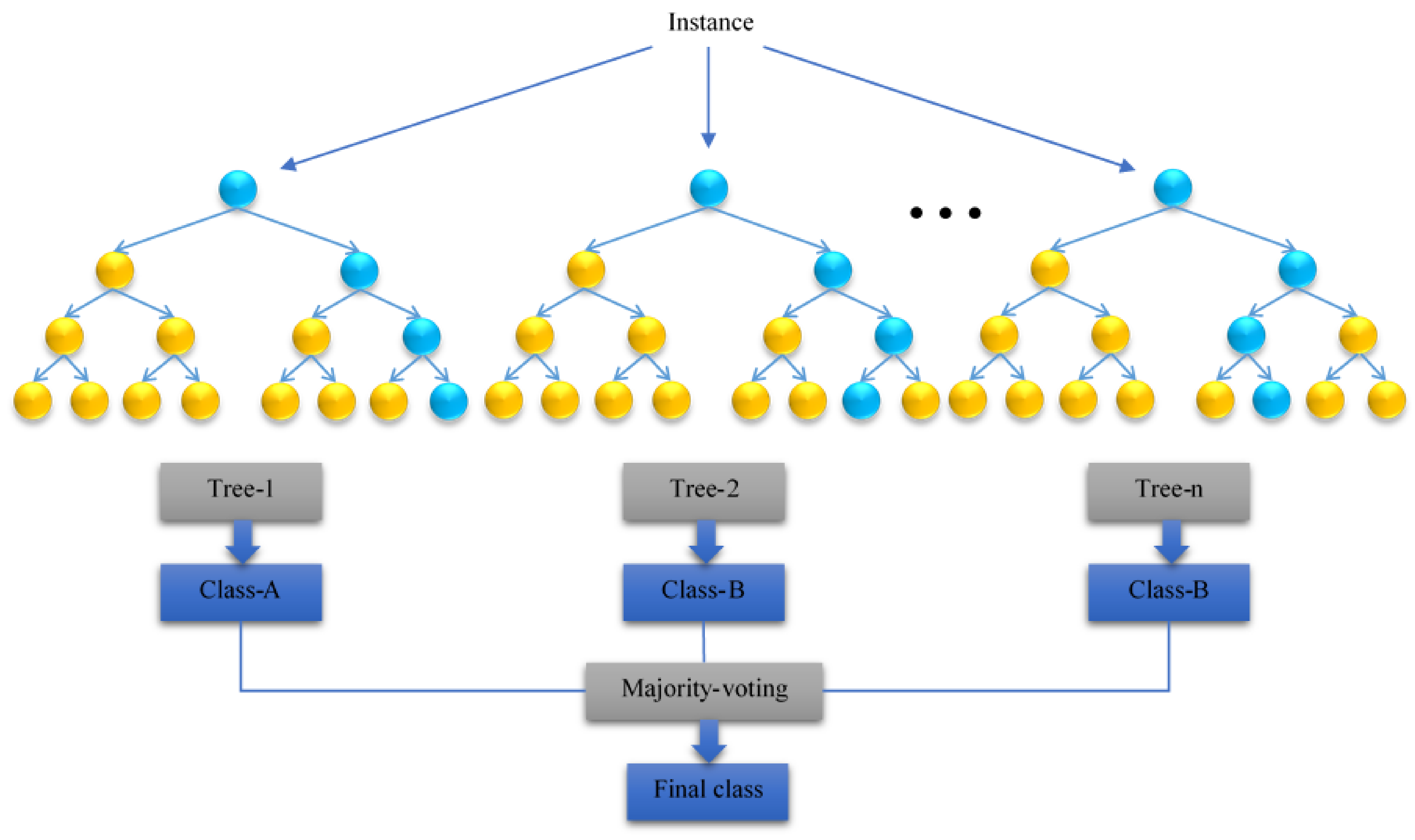
3.1.6. Random Forest

Random forest is a supervised ML algorithm that is utilized in regression and classification problems. This algorithm ensemble a number of trees and allows the trees vote for better parameters. This algorithm utilizes random selection and bagging combinations for the growth of each tree (without replacement) and is made from training dataset samples.

Amit and Geman [53], in 1997, used a large number of geometric features and a random selection search for best splitting at any node. Nature and dimensionality make up the tree structures. After the training data set is identified, the samples are randomly selected from the training data set, which creates a lot of trees. Then, they vote for the most important regression. This method is called random forest. The random forest is predicted by the average over i of the trees $\left\{h\left(x,i\right)\right\}$.

Regression random forest is defined as an ensemble learning method and makes a lot of regression tree models built from bootstrap samples of the training data [54]. Several regression tree estimators are combined to decrease the estimation error and improve the estimation precision. In this approach, the averaging of all the individual regression tree estimators is used for the estimated value. The free parameters of the method that can be optimized include the count of estimator variables randomly chosen at each node, the number of trees, the minimum leaf, the minimum count of observations in a regression tree’s terminal node, and the proportion of observations to sample in each regression tree [54,55]. The random forest procedure is illustrated in Figure 3.

3.2. Optimization Methods

3.2.1. Colliding Bodies Optimization (CBO)

CBO is a model that can be coupled with ANFIS. Kaveh and Mahdavi [56] established CBO as a novel metaheuristic search algorithm. It is based on colliding one object with another object while moving towards a minimum energy level. The concept of CBO is simple and does not depend on any internal parameter. Each colliding body (CB), Xi, owns a specific mass defined as:

$${\mathrm{M}}_{\mathrm{k}}=\frac{\frac{1}{\mathrm{fit}\left(\mathrm{k}\right) }}{{{\displaystyle \sum }}_{\mathrm{i}=1}^{\mathrm{n}}\frac{1}{\mathrm{fit}\left(\mathrm{i}\right)}}$$

(20)

where n denotes the count of colliding bodies and fit(i) is the objective function value of the ith CB. Each agent is modeled as a body with a velocity and specific mass. The end collision between pairs of objects finds the near-global or global solutions. For saving some of the best solutions, enhanced colliding bodies optimization (ECBO) utilizes memory and employs a mechanism to flee from local optima [56,57]. Figure 4 represents the flowchart of the ECBO algorithm. CBO uses a simple formulation to discover the maximum or minimum of functions and does not hinge on internal parameters.

3.2.2. Particle Swarm Optimization (PSO) Algorithm

Kennedy and Eberhart [58] developed this algorithm considering the natural swarming of insects and birds. This algorithm makes a population and selects random solutions, then, with updating the generation, the optimum solution is developed. Particles are defined as the solutions in the problem space and move towards finding the optimum answers. Each particle has position and velocity, and their positions are changed for getting well-fitness. Particles have two distinct data: (1) The best position for each particle (pbest) and (2) the global best position for the population (gbest) [59]. PSO is run and pbest and gbest are compared for avoiding local optima. The following equations, explain the updated position of the particles:

$${\nu }_i\left(t+1\right)=w·{\nu }_i\left(t\right)+c_1·ran{d}_1·(pbes{t}_i\left(t\right)-x_i\left(t\right))+c_2·ran{d}_2·(gbes{t}_i\left(t\right)-x_i\left(t\right))$$

(21)

$$x_i\left(t+1\right)=x_i\left(t\right)+{\nu }_i\left(t+1\right)(\mathrm{i}=1, \dots , \mathrm{N})$$

(22)

Here, υ is the velocity of the particle, w shows inertia weight and controls the previous velocities’ impact on new particles, N denotes the count of particles, x displays particle position, c₁ and c₂ are the learning factors and the effect of the social and cognitive components, and rand₁ and rand₂ are selected randomly [59,60,61]. The main goal of the PSO is to optimize the position of the particles according to the above equations.

3.2.3. Coupled Simulated Annealing (CSA)

CSA modifies simulated annealing for outcomes that are more precise without losing convergence speed. This modification achieves easier and better results. Besides, it accelerates the convergence of the problem. This technique is utilized for optimizing the tuning parameters of LSSVM, including γ and σ². Suykens and Vandewalle [62] displayed escaping from the local minimum for nonconvex problems as an outcome of coupling the local optimization.

3.2.4. Levenberg–Marquardt (LM) Algorithm

The MLP method uses the following algorithm and methods to improve the coefficients. The LM algorithm is one of the most practical algorithms used for optimizing the weights and biases of MLP models. Solving nonlinear least squares problems is done with this algorithm. More details about this algorithm are available in the literature [63,64].

4. Results and Discussion

4.1. Comparison of ML Models

The data were divided into two subsets, including training data (80% of the data) and testing data (20% of the data). Parameter setting in all models is done manually using a trial-and-error approach according to the amount of data. However, after setting the input parameters to start modeling, the model adjusts its internal parameters to achieve the best output in the shortest time. Effective input parameters are modified to match the output with the target data after each model is run. In this case, there are four inputs and one output, but the models have their own parameters that are adjusted based on the structure of their formation. For example, in order to create a fitting network in MLP, the number of hidden layers and the number of neurons in every hidden layer are determined by applying a trial-and-error approach. ANFIS relies on the number of repetitions and the population. LSSVM uses the tune LSSVM function to communicate with input data and calls the optimal regularization parameter and the optimal kernel parameter(s). RBF also regulates the maximum count of neurons and the coefficient spread. After modeling, the following results were found to be appropriate and lead to the best structure in each model. LM was used to optimize the MLP parameters (biases and weights). The best structure of the MLP was obtained as size = (20 12), which denotes a model with two hidden layers having 20 and 12 neurons. Likewise, the number of extra-trees in the ensemble was obtained at 40. The population in ANIFS–PSO and ANFIS–ECBO were 40 and 20, respectively. The best results of both algorithms were attained after 1000 and 2000 iterations, respectively. The number of input parameters is four for all algorithms. In the RBF algorithm, the maximum count of neurons was 100, and the spread coefficient was 2. Moreover, the random forest used 150 bags for tree bagging. The optimal regularization and optimal kernel parameters of the LSSVM are 962,599.26 and 3.554, respectively.

The validity and accuracy of a model is identified by the error between the output (y_cal) and target (y_exp) data. Several statistical criteria were employed to recognize these errors and to prove the validity of the developed models. These statistical criteria include [65]:

• Average percent relative error (APRE%):

  $$\mathrm{APRE}=\frac{1}{n} {\displaystyle \sum }_{i=1}^n\frac{\left(y_{exp}-y_{cal}\right)}{\left(y_{exp}\right)}\times 100$$

  (23)
• Average absolute percent relative error (AAPRE%):

  $$\mathrm{AAPRE}=\frac{1}{n} {\displaystyle \sum }_{i=1}^n\left|\frac{\left(y_{exp}-y_{cal}\right)}{\left(y_{exp}\right)}\times 100\right|$$

  (24)
• Root mean square error (RMSE):

  $$\mathrm{RMSE}=\sqrt{\frac{{{\displaystyle \sum }}_{i=1}^n(y_{exp-}{y}_{cal)}{}^2}{n}}$$

  (25)
• Standard errors (SD):

  $$\mathrm{SD}=\sqrt{\frac{{{\displaystyle \sum }}_{i=1}^n{\frac{(y_{exp-}{y}_{cal) }}{y_{exp}}}^2}{n-1}}$$

  (26)

According to the calculated statistical criteria of the models represented in

Table 2. Statistical parameters for the proposed models in this work.

R2	SD	APRE %	AAPRE %	RMSE		Statistical Factor
0.996	0.0263	−0.0100	1.9147	0.282	Train	ANFIS–PSO
0.989	0.0476	−0.3639	3.241	0.5458	Test
0.994	0.0982	−0.0814	2.182	0.3515	Total
0.988	0.0423	0.1674	3.206	0.4846	Train	ANFIS–ECBO
0.988	0.0597	2.0286	4.0881	0.5802	Test
0.988	0.1441	0.5424	3.3838	0.5053	Total
0.999	0.0065	−0.0001	0.389	0.0645	Train	MLP–LM
0.996	0.0256	0.2437	1.991	0.2837	Test
0.998	0.0429	0.0919	0.7868	0.154	Total
0.999	0.0101	−0.0110	0.7061	0.1102	Train	LSSVM–CSA
0.998	0.0146	0.1029	1.1449	0.1638	Test
0.999	0.0359	0.0119	0.7945	0.1229	Total
0.999	0.0098	−0.0090	0.6844	0.1017	Train	RBF
0.998	0.0152	0.3838	1.1479	0.1569	Test
0.999	0.0341	0.0701	0.7778	0.115	Total
0.999	0.0207	−0.2573	1.1612	0.1386	Train	Extra-tree
0.991	0.0527	−0.8242	3.5599	0.4361	Test
0.997	0.0759	−0.3716	1.6445	0.2317	Total
0.984	0.102	−1.7619	4.9478	0.755	Train	Random forest
0.965	0.0795	−1.7963	5.9719	0.619	Test
0.981	0.2183	−1.7689	5.1542	0.6487	Total

, RBF has shown the best results. As shown in Table 2, the RBF model has the least AAPRE (0.77%) and RMSE (0.11 mN·m⁻¹) compared to other models. Furthermore, LSSVM–CSA, MLP–LM, extra-tree, ANFIS–PSO, ANFIS–ECBO, and the random forest models have the best accuracy following the RBF model. The run time is another important parameter that affects selecting the best model in soft computing efforts. Figure 5 depicts the statistical results of the run time and the computational accuracy for the various methods, which reveals that the RBF is the best model in this study, having a minimum AAPRE (0.77%) and run time (36 s).

The following graphical diagrams were used to visually demonstrate the performance and accuracy of the models:

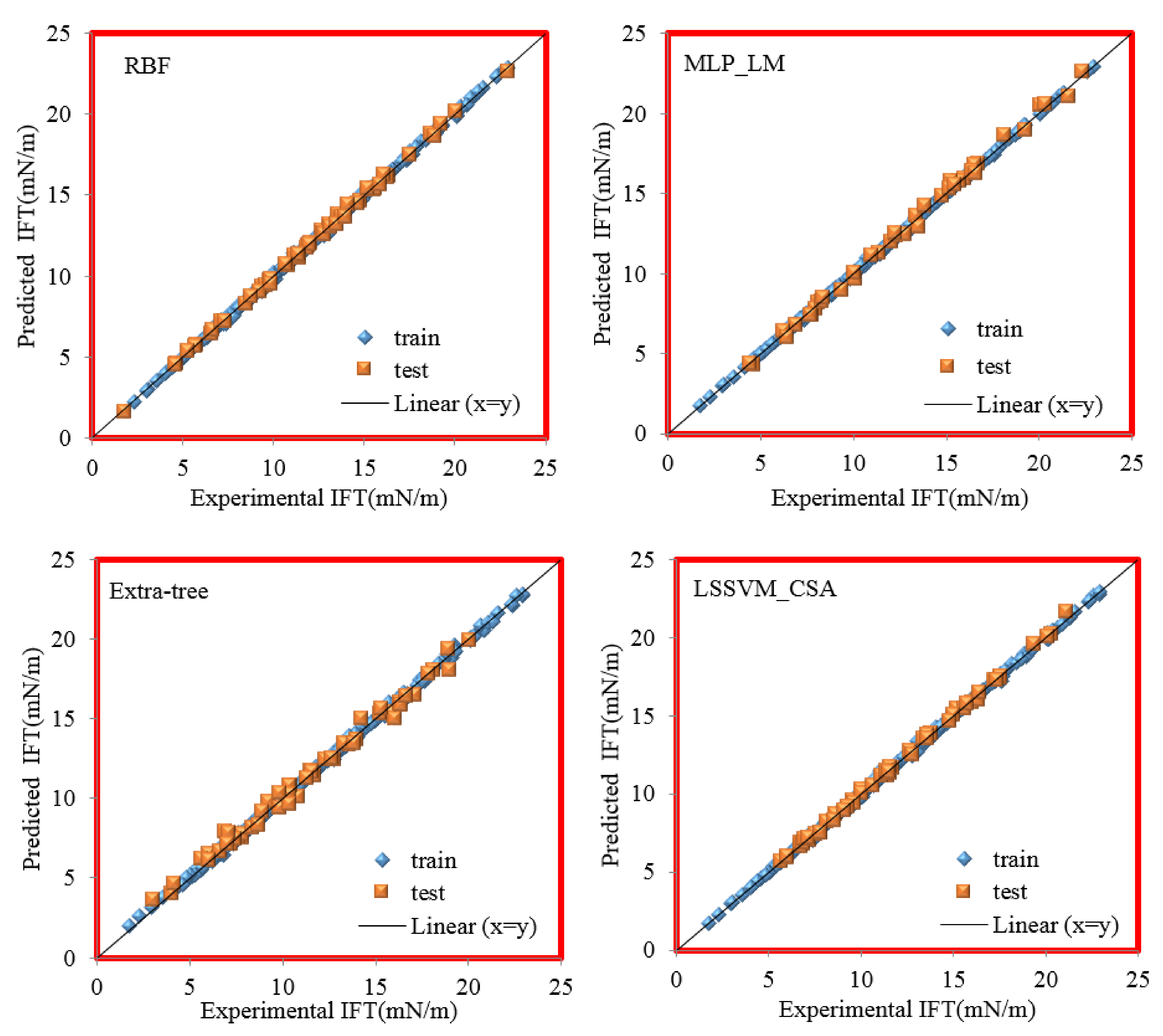
• Cross plot: In this graph, the estimated data by the models are plotted versus the laboratory data. Using this visual presentation, we can assess the deviation of the estimated data by the models from the actual data. The more data near the unit slope line, the greater the precision of the model in predicting the experimental data would be. Figure 6 displays the comparison between the output and target data by cross plots for all models. As can be seen, the data points are located near the unit slope line for the ML models, although the precision of the RBF, LSSVM–CSA, and MLP–LM models is higher for both testing and training sets.
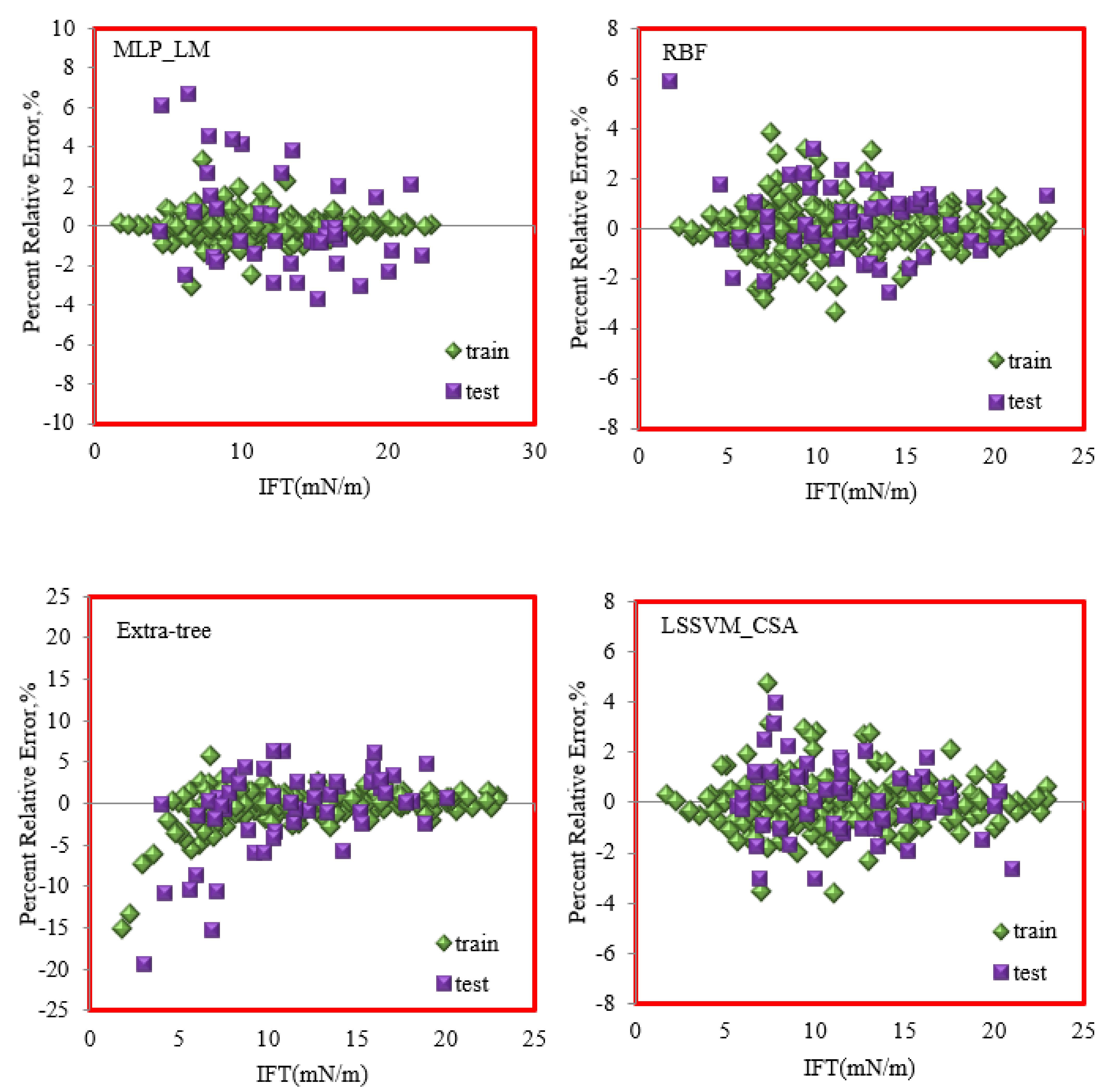
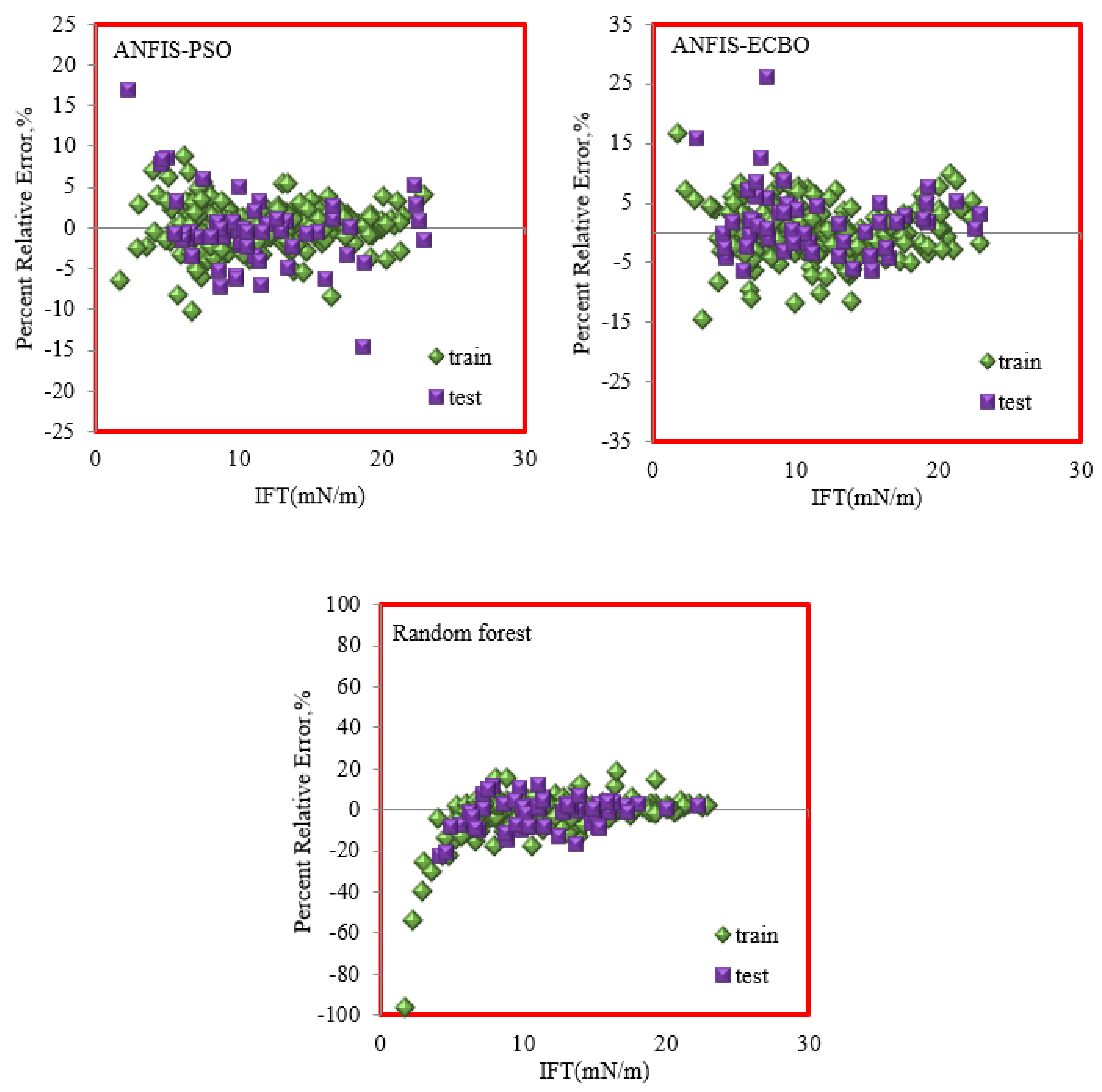
• Error distribution plot: This plot explains the percent relative error of each data point versus the real laboratory data or the independent parameters so to represent the error value or the possible error trend. If the error value is close to nil, it reveals that the estimated data and the laboratory data are close to each other, but the high scatter of the data around the zero-error line infers the poor performance of the model. Figure 7 depicts the error distribution plots for all proposed models in this work. Similarly, RBF and LSSVM–CSA are considered more precise models, having more data points with less error and a high concentration of data near the zero-error line.
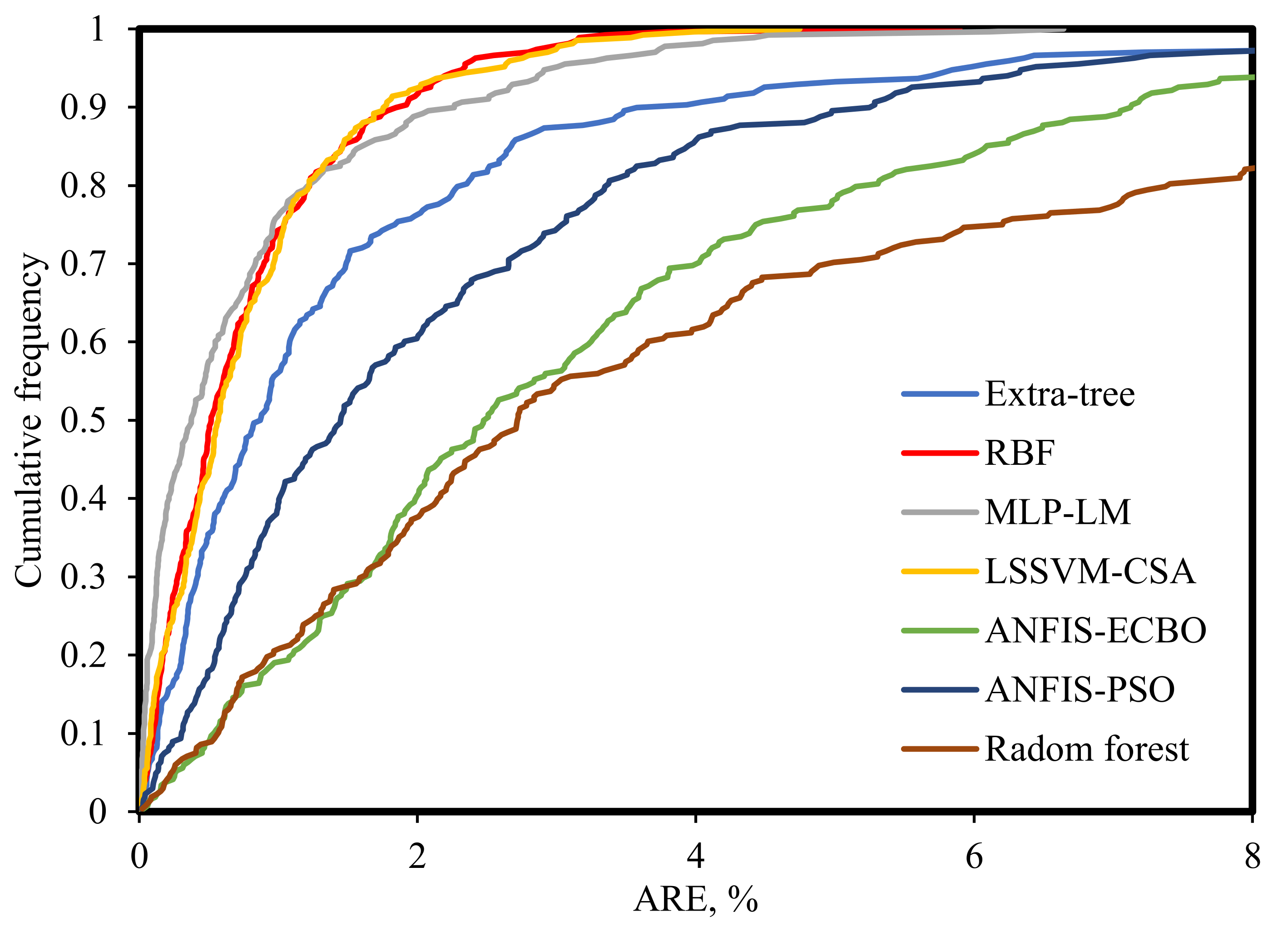
• Cumulative frequency plot: The error of each model in estimating any percentage of the data can be examined by plotting the cumulative frequency vs. the absolute relative error (ARE, %). Cumulative frequency graphs of all models are shown in Figure 8. The robustness of the RBF model is acceptable, since about 90% of the data have ARE lower than 1.8%. Moreover, the LSSVM–CSA and MLP–LM models have a high percentage of low-error data, which confirms the high reliability of these models along with the RBF model. The random forest and ANFIS–ECBO models display poorer performance compared to other ones.

Figure 9 depicts the AAPRE of the proposed models in this work and the empirical correlation of Shang et al. [36] in predicting the IFT of the N₂/CO₂ mixture + n-alkanes. All models proposed in this paper except the Random-forest model have a lower AAPRE than the proposed Shang et al. correlation. RBF, LSSVM–CSA, and MLP–LM models are more accurate than other models and correlation in estimating the IFT of the N₂/CO₂ mixture + n-alkanes.

After evaluating all proposed models, RBF was selected as the best model for estimating the IFT of the N₂/CO₂ mixture + n-alkanes. Hence, further analyses were performed with this model.

4.2. Trend Analysis

In the next step, the IFT of the N₂/CO₂ mixture + n-hexane [36] was estimated with the RBF model to assess the ability of this model in predicting the actual physical process of IFT changes at different pressures and temperatures. Figure 10 depicts the experimental IFT of N₂/CO₂ mixture + n-hexane and RBF model predictions. Based on the results, when pressure increased, the IFT decreased because pressure rising caused increasing forces on the fluid surface, which makes a minimum surface that is contacted with other fluid or solid surfaces. Increasing the temperature also has a decreasing effect on the IFT of the N₂/CO₂ mixture + n-hexane. Here, the RBF model correctly estimates the IFT of the N₂/CO₂ mixture + n-hexane at different operating conditions and demonstrates the superior ability to track the process of decreasing IFT with increasing pressure and temperature.

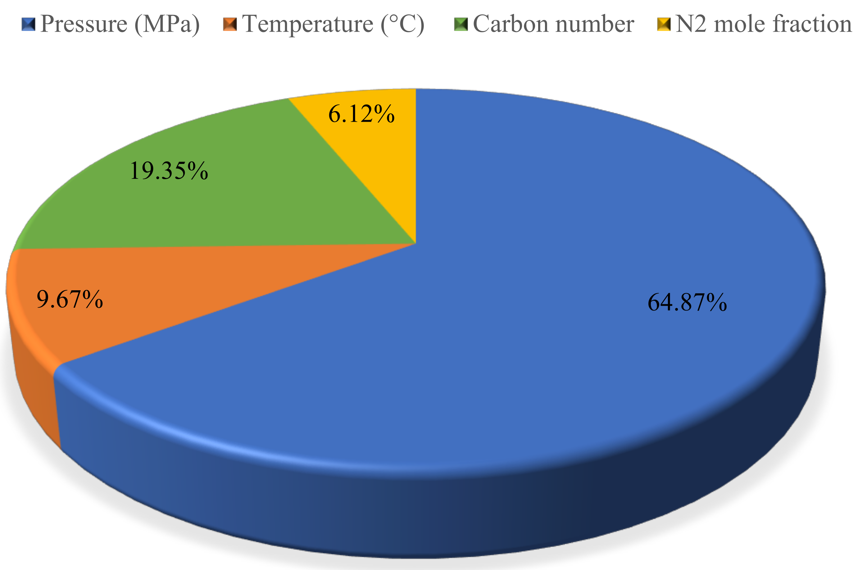
4.3. Sensitivity Analysis

In the next stage, the relevancy factor (r) is analyzed to assess the quantitative influence of inputs on the outcome of the RBF model. The higher r-value for an input variable indicates the higher impact of that parameter on the IFT of the N₂/CO₂ mixture + n-alkanes. The r-values for the input parameters that can be calculated using the equation below [66]:

$$r\left(in{p}_i,IFT\right)=\frac{{{\displaystyle \sum }}_{j=1}^n\left(in{p}_{i,j}-in{p}_{ave,i}\right)\left(IF{T}_j-IF{T}_{ave}\right)}{\sqrt{{{\displaystyle \sum }}_{j=1}^n{\left(in{p}_{i,j}-in{p}_{ave,i}\right)}^2{{\displaystyle \sum }}_{j=1}^n{\left(IF{T}_j-IF{T}_{ave}\right)}^2}}$$

(27)

where inp_ave,i and inp_i,j stand for the average value and the jth value of the ith input, respectively (i is pressure, temperature, the mole fraction of N₂, and the carbon number of n-alkanes). IFT_j stands for the jth value of the prognosticated IFTm and IFT_ave is the average of prognosticated IFT of the N₂/CO₂ mixture + n-alkanes. The effect of the input variables on the IFT of the N₂/CO₂ mixture + n-alkanes is presented in Figure 11 in percentages. As shown in this figure, pressure had the greatest influence on the IFT of the N₂/CO₂ mixture + n-alkanes, followed by carbon number of n-alkanes, the temperature, and the mole fraction of N₂.

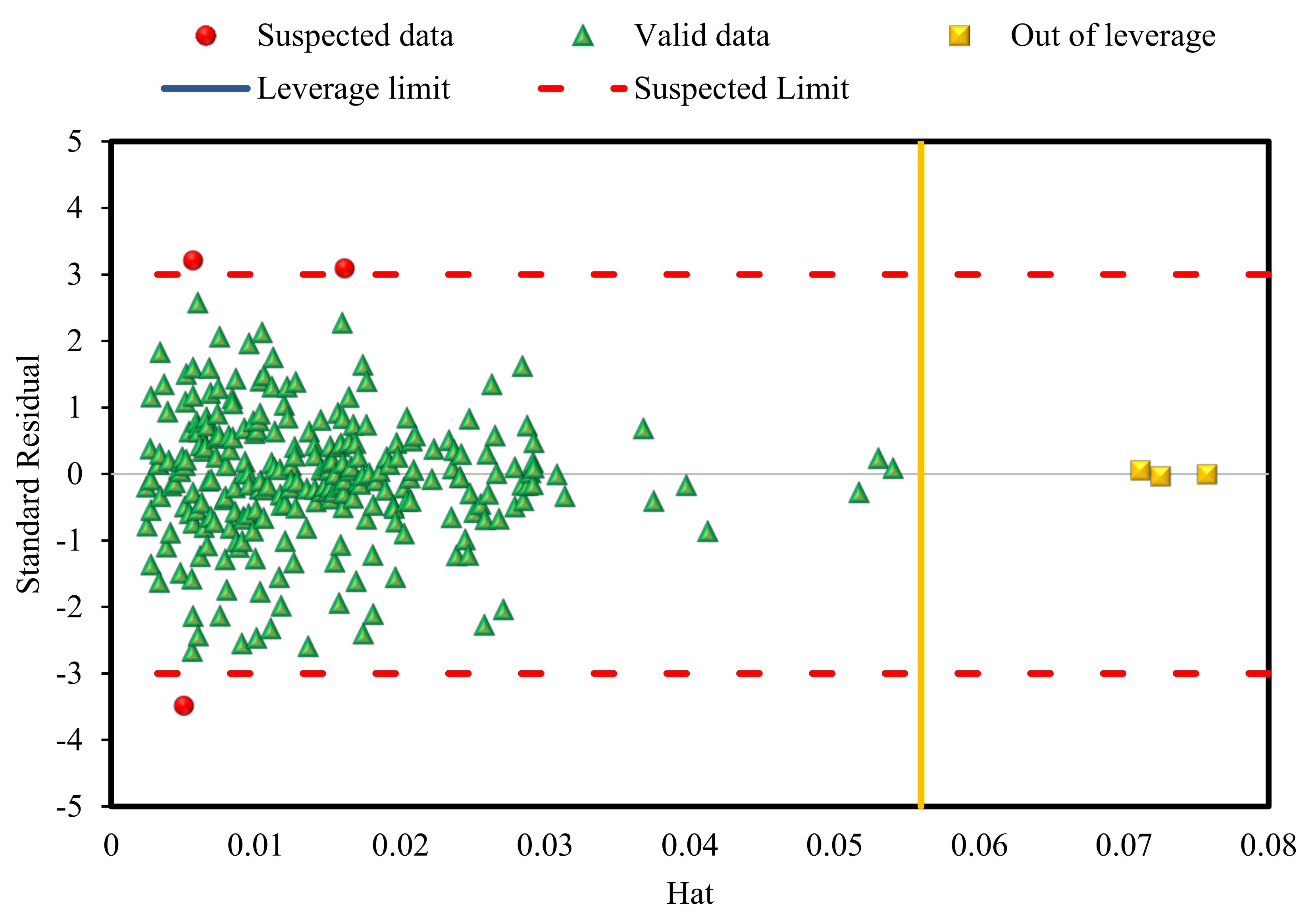
4.4. Model Reliability Assessment and Outlier Diagnostics

Utilizing the leverage approach [67,68,69] as a technique to determine the applicability area of a model and the probable outlier data can give a good view of the validity of the RBF model. In this method, the deviations of the output of the model from the real data are standardized residuals (R), and Hat matrix leverage values are computed. The usability area of the model is also determined graphically by plotting the William’s plot. Figure 12 depicts the obtained William’s plot for the RBF model, in which the Hat matrix leverage (H) values and critical leverage (H*) were distinguished. As can be seen in Figure 12, the majority of the data are located in the interval of −3 ≤ R ≤ 3 and 0 ≤ H ≤ H*. The points with lower values of R and H are more reliable [70,71]. Only six data points were recognized to be outside of the scope of the model applicability, which proves the high reliability of the RBF model for estimating the IFT of the N₂/CO₂ mixture + n-alkanes. The data points that are out of the scope of the model’s application are presented in

Table 3. Detected suspected data or outliers for the RBF model according to the leverage approach.

Reference	R	H	IFT,	IFT,	Pressure (MPa)	Temperature	N2 (Mole Fraction)	Carbon Number	No.
			Pred. (mN/m)	Exp. (mN/m)		(°C)
[36]	3.204	0.00571	11.4096	11.04	8.01	60	0.25	13	1
[36]	−3.4922	0.00509	12.6572	13.06	6.96	80	0.25	13	2
[36]	3.0862	0.01619	14.4079	14.05	5.97	40	0.25	15	3
[39]	−0.0127	0.0758	2.2784	2.28	40.16	40	1	6	4
[39]	−0.0398	0.0725	5.6152	5.62	40.1	40	1	8	5
[39]	0.04771	0.0711	8.0556	8.05	40.1	40	1	10	6

. Collectively, this study showed how using AI would enable us to predict the IFT of various gas mixtures in different pressures and temperatures so to ultimately make us independent from running expensive and time consuming experimental studies or to avoid the numerical methods that can be less precise.

5. Conclusions

In the current paper, the IFT of the CO₂/N₂ mixture and n-alkanes was modeled utilizing ML methods at different pressures and temperatures. A data set containing 268 IFT data was gathered from the literature. The pressure, temperature, carbon number, and the mole fraction of N₂ were selected as input parameters. Six well-known ML methods, RBF, LSSVM, ANFIS, MLP, random-forest, and extra-tree, were used along with four optimization techniques, CBO, the LM algorithm, PSO, and CSA, to model the IFT between the CO₂/N₂ mixture and n-alkanes. Based on the results the following conclusions are made:

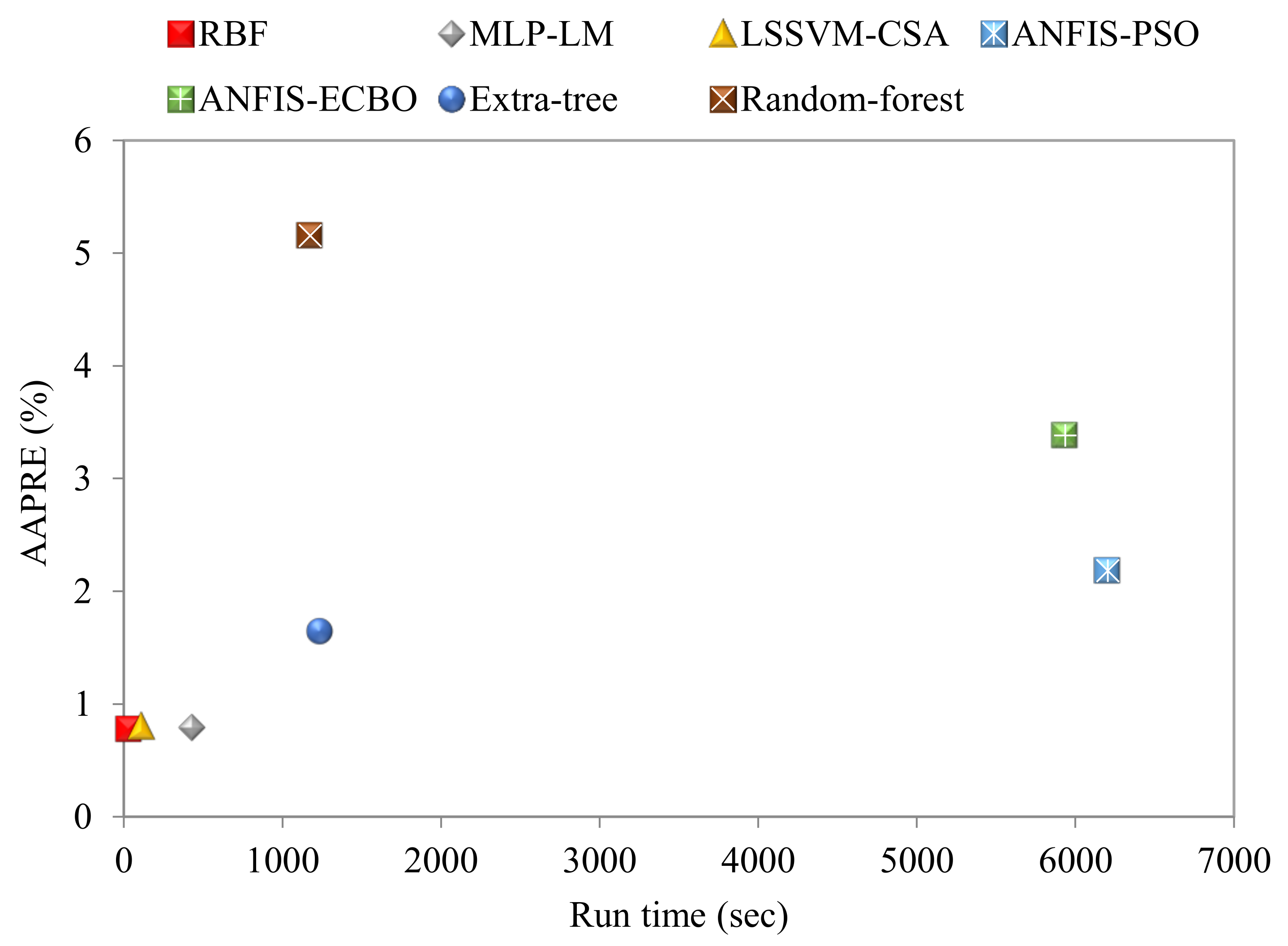
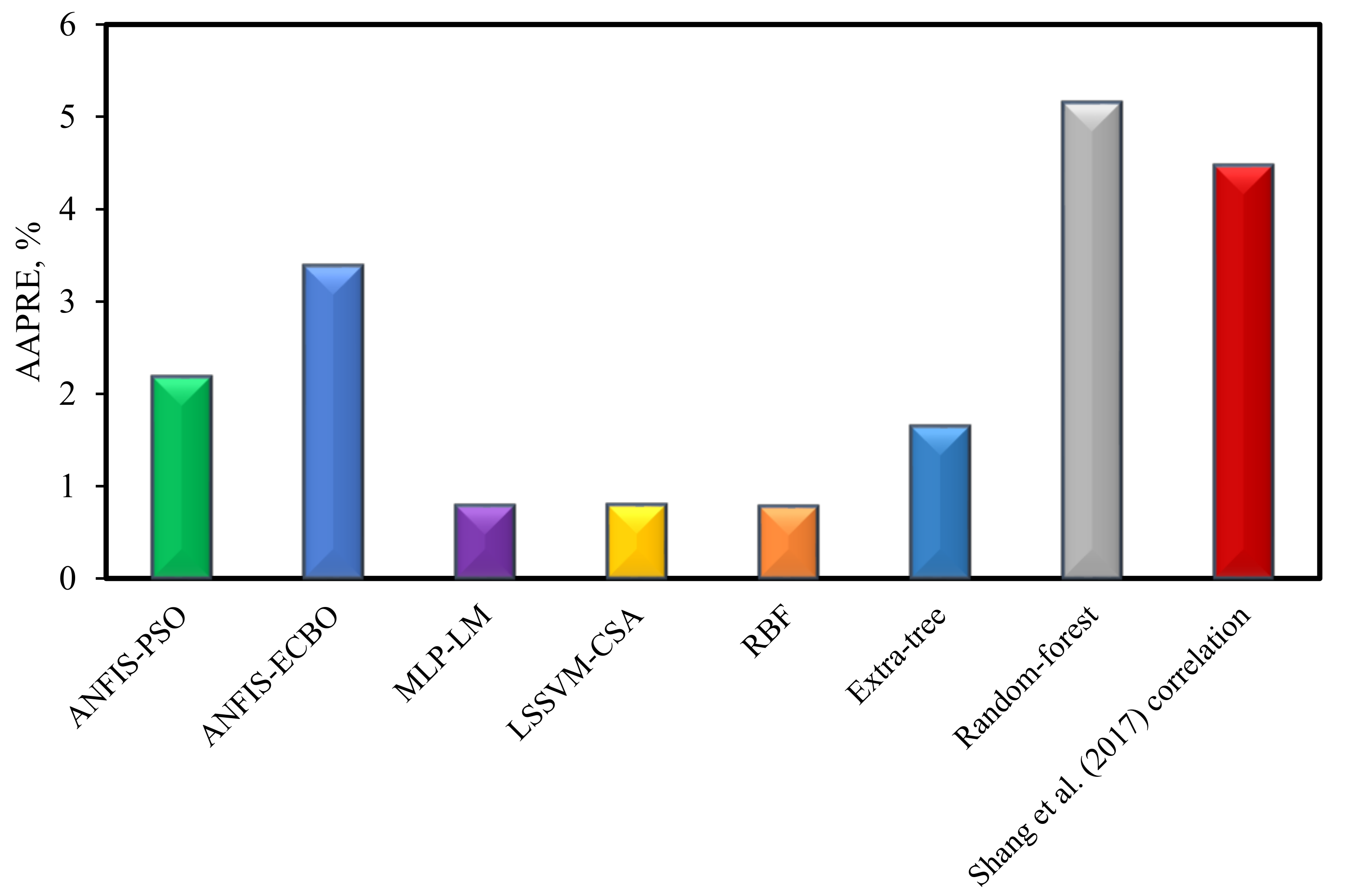
• The RBF model estimates all of the IFT data with superb accuracy, with an AAPRE of 0.77%, which outperformed all proposed models in this work and the literature. The RBF model successfully recognized the decreasing trend of IFT with increasing pressure and temperature.
• Moreover, LSSVM–CSA, MLP–LM, extra-tree, ANFIS–PSO, ANFIS–ECBO, and random-forest models followed the RBF model in terms of accuracy.
• According to the sensitivity analysis, pressure would have the greatest impact on the IFT of the N₂/CO₂ mixture + n-alkanes, followed by carbon number of n-alkanes, the temperature, and the mole fraction of N₂y. Pressure and temperature have a decreasing impact on the IFT of the N₂/CO₂ mixture + n-alkanes.
• Finally, based on the leverage approach, only six data points were recognized to be outside of the scope of the model applicability, which proves the high reliability of the RBF model for estimating the IFT of the N₂/CO₂ mixture + n-alkanes.

References

1. Ameli, F.; Hemmati-Sarapardeh, A.; Schaffie, M.; Husein, M.M.; Shamshirband, S. Modeling interfacial tension in N2/n-alkane systems using corresponding state theory: Application to gas injection processes. Fuel 2018, 222, 779–791. [Google Scholar] [CrossRef]
2. Bakyani, A.E.; Namdarpoor, A.; Sarvestani, A.N.; Daili, A.; Raji, B.; Esmaeilzadeh, F. A Simulation Approach for Screening of EOR Scenarios in Naturally Fractured Reservoirs. Int. J. Geosci. 2018, 9, 19–43. [Google Scholar] [CrossRef] [Green Version]
3. Al Adasani, A.; Bai, B. Analysis of EOR projects and updated screening criteria. J. Pet. Sci. Eng. 2011, 79, 10–24. [Google Scholar] [CrossRef]
4. Gajbhiye, R. Effect of CO2/N2 Mixture Composition on Interfacial Tension of Crude Oil. ACS Omega 2020, 5, 27944–27952. [Google Scholar] [CrossRef] [PubMed]
5. Bender, S. Co-Optimization of CO2 Sequestration and Enhanced Oil Recovery and Co-Optimization of CO2 Sequestration and Methane Recovery in Geopressured Aquifers. Ph.D. Thesis, The University of Texas at Austin, Austin, TX, USA, 2011. [Google Scholar]
6. Bender, S.; Akin, S. Flue gas injection for EOR and sequestration: Case study. J. Pet. Sci. Eng. 2017, 157, 1033–1045. [Google Scholar] [CrossRef]
7. Roefs, P.; Moretti, M.; Welkenhuysen, K.; Piessens, K.; Compernolle, T. CO2-enhanced oil recovery and CO2 capture and storage: An environmental economic trade-off analysis. J. Environ. Manag. 2019, 239, 167–177. [Google Scholar] [CrossRef]
8. Du, F.; Nojabaei, B. A Review of Gas Injection in Shale Reservoirs: Enhanced Oil/Gas Recovery Approaches and Greenhouse Gas Control. Energies 2019, 12, 2355. [Google Scholar] [CrossRef] [Green Version]
9. Hoffman, B.T. Comparison of Various Gases for Enhanced Recovery from Shale Oil Reservoirs. In Proceedings of the SPE Improved Oil Recovery Symposium, Tulsa, OK, USA, 14–18 April 2012. [Google Scholar]
10. Ratner, M.; Tiemann, M. An Overview of Unconventional Oil and Natural Gas: Resources and Federal Actions; Congressional Research Service: Washington, DC, USA, 2014.
11. Jin, L.; Hawthorne, S.; Sorensen, J.; Pekot, L.; Kurz, B.; Smith, S.; Heebink, L.; Bosshart, N.; Torres, J.; Dalkhaa, C.; et al. Extraction of oil from the Bakken shales with supercritical CO2. In Proceedings of the SPE/AAPG/SEG Unconventional Resources Technology Conference, Austin, TX, USA, 17–21 July 2017. [Google Scholar]
12. Fathi, E.; Akkutlu, I.Y. Multi-component gas transport and adsorption effects during CO2 injection and enhanced shale gas recovery. Int. J. Coal Geol. 2013, 123, 52–61. [Google Scholar] [CrossRef]
13. Yu, W.; Lashgari, H.R.; Wu, K.; Sepehrnoori, K. CO2 injection for enhanced oil recovery in Bakken tight oil reservoirs. Fuel 2015, 159, 354–363. [Google Scholar] [CrossRef]
14. Fathi, E.; Akkutlu, I.Y. Mass Transport of Adsorbed-Phase in Stochastic Porous Medium with Fluctuating Porosity Field and Nonlinear Gas Adsorption Kinetics. Transp. Porous Media 2011, 91, 5–33. [Google Scholar] [CrossRef]
15. Yang, J.; Okwananke, A.; Tohidi, B.; Chuvilin, E.; Maerle, K.; Istomin, V.; Bukhanov, B.; Cheremisin, A. Flue gas injection into gas hydrate reservoirs for methane recovery and carbon dioxide sequestration. Energy Convers. Manag. 2017, 136, 431–438. [Google Scholar] [CrossRef]
16. Sloan, E.D., Jr.; Koh, C.A. Clathrate Hydrates of Natural Gases; CRC Press: Boca Raton, FL, USA, 2007. [Google Scholar]
17. Rezaei, F.; Rezaei, A.; Jafari, S.; Hemmati-Sarapardeh, A.; Mohammadi, A.H.; Zendehboudi, S. On the Evaluation of Interfacial Tension (IFT) of CO2–Paraffin System for Enhanced Oil Recovery Process: Comparison of Empirical Correlations, Soft Computing Approaches, and Parachor Model. Energies 2021, 14, 3045. [Google Scholar] [CrossRef]
18. Ghosh, A.; Chakraborty, D.; Law, A. Artificial intelligence in Internet of things. CAAI Trans. Intell. Technol. 2018, 3, 208–218. [Google Scholar] [CrossRef]
19. Kalogirou, S. Applications of artificial neural-networks for energy systems. Appl. Energy 2000, 67, 17–35. [Google Scholar] [CrossRef]
20. Ongsulee, P. Artificial intelligence, machine learning and deep learning. In Proceedings of the 15th International Conference on ICT and Knowledge Engineering (ICT&KE), Bangkok, Thailand, 22–24 November 2017; pp. 1–6. [Google Scholar]
21. Janiesch, C.; Zschech, P.; Heinrich, K. Machine learning and deep learning. Electron. Mark. 2021, 31, 685–695. [Google Scholar] [CrossRef]
22. Barati-Harooni, A.; Soleymanzadeh, A.; Tatar, A.; Najafi-Marghmaleki, A.; Samadi, S.-J.; Yari, A.; Roushani, B.; Mohammadi, A.H. Experimental and modeling studies on the effects of temperature, pressure and brine salinity on interfacial tension in live oil-brine systems. J. Mol. Liq. 2016, 219, 985–993. [Google Scholar] [CrossRef]
23. Amar, M.N.; Shateri, M.; Hemmati-Sarapardeh, A.; Alamatsaz, A. Modeling oil-brine interfacial tension at high pressure and high salinity conditions. J. Pet. Sci. Eng. 2019, 183, 106413. [Google Scholar] [CrossRef]
24. Meybodi, M.K.; Shokrollahi, A.; Safari, H.; Lee, M.; Bahadori, A. A computational intelligence scheme for prediction of interfacial tension between pure hydrocarbons and water. Chem. Eng. Res. Des. 2015, 95, 79–92. [Google Scholar] [CrossRef]
25. Najafi-Marghmaleki, A.; Tatar, A.; Barati-Harooni, A.; Mohebbi, A.; Kalantari-Meybodi, M.; Mohammadi, A.H. On the prediction of interfacial tension (IFT) for water-hydrocarbon gas system. J. Mol. Liq. 2016, 224, 976–990. [Google Scholar] [CrossRef]
26. Emami Baghdadi, M.H.; Darvish, H.; Rezaei, H.; Savadinezhad, M. Applying LSSVM algorithm as a novel and accurate method for estimation of interfacial tension of brine and hydrocarbons. Pet. Sci. Technol. 2018, 36, 1170–1174. [Google Scholar] [CrossRef]
27. Darvish, H.; Rahmani, S.; Sadeghi, A.M.; Baghdadi, M.H.E. The ANFIS-PSO strategy as a novel method to predict interfacial tension of hydrocarbons and brine. Pet. Sci. Technol. 2018, 36, 654–659. [Google Scholar] [CrossRef]
28. Mehrjoo, H.; Riazi, M.; Amar, M.N.; Hemmati-Sarapardeh, A. Modeling interfacial tension of methane-brine systems at high pressure and high salinity conditions. J. Taiwan Inst. Chem. Eng. 2020, 114, 125–141. [Google Scholar] [CrossRef]
29. Niroomand-Toomaj, E.; Etemadi, A.; Shokrollahi, A. Radial basis function modeling approach to prognosticate the interfacial tension CO2/Aquifer Brine. J. Mol. Liq. 2017, 238, 540–544. [Google Scholar] [CrossRef]
30. Kamari, A.; Pournik, M.; Rostami, A.; Amirlatifi, A.; Mohammadi, A.H. Characterizing the CO2-brine interfacial tension (IFT) using robust modeling approaches: A comparative study. J. Mol. Liq. 2017, 246, 32–38. [Google Scholar] [CrossRef]
31. Liu, X.; Mutailipu, M.; Zhao, J.; Liu, Y. Comparative Analysis of Four Neural Network Models on the Estimation of CO2–Brine Interfacial Tension. ACS Omega 2021, 6, 4282–4288. [Google Scholar] [CrossRef] [PubMed]
32. Amar, M.N. Towards improved genetic programming based-correlations for predicting the interfacial tension of the systems pure/impure CO2-brine. J. Taiwan Inst. Chem. Eng. 2021, 127, 186–196. [Google Scholar] [CrossRef]
33. Ahmadi, M.A.; Mahmoudi, B. Development of robust model to estimate gas–oil interfacial tension using least square support vector machine: Experimental and modeling study. J. Supercrit. Fluids 2016, 107, 122–128. [Google Scholar] [CrossRef]
34. Ayatollahi, S.; Hemmati-Sarapardeh, A.; Roham, M.; Hajirezaie, S. A rigorous approach for determining interfacial tension and minimum miscibility pressure in paraffin-CO2 systems: Application to gas injection processes. J. Taiwan Inst. Chem. Eng. 2016, 63, 107–115. [Google Scholar] [CrossRef]
35. Hemmati-Sarapardeh, A.; Mohagheghian, E. Modeling interfacial tension and minimum miscibility pressure in paraffin-nitrogen systems: Application to gas injection processes. Fuel 2017, 205, 80–89. [Google Scholar] [CrossRef]
36. Shang, Q.; Xia, S.; Cui, G.; Tang, B.; Ma, P. Measurement and correlation of the interfacial tension for paraffin + CO2 and (CO2 +N2) mixture gas at elevated temperatures and pressures. Fluid Phase Equilib. 2017, 439, 18–23. [Google Scholar] [CrossRef]
37. Zhang, J.; Sun, Y.; Shang, L.; Feng, Q.; Gong, L.; Wu, K. A unified intelligent model for estimating the (gas + n-alkane) interfacial tension based on the eXtreme gradient boosting (XGBoost) trees. Fuel 2020, 282, 118783. [Google Scholar] [CrossRef]
38. Mirzaie, M.; Tatar, A. Modeling of interfacial tension in binary mixtures of CH4, CO2, and N2-alkanes using gene expression programming and equation of state. J. Mol. Liq. 2020, 320, 114454. [Google Scholar] [CrossRef]
39. Jianhua, T.; Satherley, J.; Schiffrin, D. Density and intefacial tension of nitrogen-hydrocarbon systems at elevated pressures. Chin. J. Chem. Eng. 1993, 1, 223–231. [Google Scholar]
40. Wehle, H.-D. Machine Learning, Deep Learning and AI: What’s the Difference. Data Scientist Innovation Day. 2017, pp. 2–5. Available online: https://www.researchgate.net/publication/318900216_Machine_Learning_Deep_Learning_and_AI_What%27s_the_Difference (accessed on 30 August 2021).
41. Mohammadi, M.-R.; Hadavimoghaddam, F.; Atashrouz, S.; Abedi, A.A.; Hemmati-Sarapardeh, A.; Mohaddespour, A. Modeling hydrogen solubility in alcohols using machine learning models and equations of state. J. Mol. Liq. 2021, 346, 117807. [Google Scholar] [CrossRef]
42. Hastie, T.; Tibshirani, R.; Friedman, J. The Elements of Statistical Learning: Data Mining, Inference, and Prediction; Springer Science & Business Media: Berlin/Heidelberg, Germany, 2009. [Google Scholar]
43. Ameli, F.; Hemmati-Sarapardeh, A.; Tatar, A.; Zanganeh, A.; Ayatollahi, S. Modeling interfacial tension of normal alkane-supercritical CO2 systems: Application to gas injection processes. Fuel 2019, 253, 1436–1445. [Google Scholar] [CrossRef]
44. Broomhead, D.; Lowe, D. Multivariable functional interpolation and adaptive networks. Complex Syst. 1988, 2, 321–355. [Google Scholar]
45. Suykens, J.A.K.; Vandewalle, J. Least Squares Support Vector Machine Classifiers. Neural Process. Lett. 1999, 9, 293–300. [Google Scholar] [CrossRef]
46. Wang, H.; Hu, D. Comparison of SVM and LS-SVM for regression. In Proceedings of the 2005 International Conference on Neural Networks and Brain, Beijing, China, 13–15 October 2005; pp. 279–283. [Google Scholar]
47. Gharagheizi, F.; Eslamimanesh, A.; Farjood, F.; Mohammadi, A.H.; Richon, D. Solubility Parameters of Nonelectrolyte Organic Compounds: Determination Using Quantitative Structure–Property Relationship Strategy. Ind. Eng. Chem. Res. 2011, 50, 11382–11395. [Google Scholar] [CrossRef]
48. Rafiee-Taghanaki, S.; Arabloo, M.; Chamkalani, A.; Amani, M.; Zargari, M.H.; Adelzadeh, M.R. Implementation of SVM framework to estimate PVT properties of reservoir oil. Fluid Phase Equilib. 2013, 346, 25–32. [Google Scholar] [CrossRef]
49. Bahadori, A.; Vuthaluru, H.B. A novel correlation for estimation of hydrate forming condition of natural gases. J. Nat. Gas Chem. 2009, 18, 453–457. [Google Scholar] [CrossRef]
50. Pelckmans, K.; Suykens, J.A.; Van Gestel, T.; De Brabanter, J.; Lukas, L.; Hamers, B.; De Moor, B.; Vandewalle, J. LS-SVMlab: A Matlab/c Toolbox for Least Squares Support Vector Machines; ESAT: Leuven, Belgium, 2002; Volume 142, pp. 1–2. [Google Scholar]
51. Zadeh, L.A. Information and control. Fuzzy Sets 1965, 8, 338–353. [Google Scholar]
52. Geurts, P.; Ernst, D.; Wehenkel, L. Extremely randomized trees. Mach. Learn. 2006, 63, 3–42. [Google Scholar] [CrossRef] [Green Version]
53. Amit, Y.; Geman, D. Shape Quantization and Recognition with Randomized Trees. Neural Comput. 1997, 9, 1545–1588. [Google Scholar] [CrossRef] [Green Version]
54. Breiman, L. Random forests. Mach. Learn. 2001, 45, 5–32. [Google Scholar] [CrossRef] [Green Version]
55. Fouedjio, F. Exact Conditioning of Regression Random Forest for Spatial Prediction. Artif. Intell. Geosci. 2020, 1, 11–23. [Google Scholar] [CrossRef]
56. Kaveh, A.; Mahdavi, V. Colliding bodies optimization: A novel meta-heuristic method. Comput. Struct. 2014, 139, 18–27. [Google Scholar] [CrossRef]
57. Kaveh, A.; Ilchi Ghazaan, M. Computer codes for colliding bodies optimization and its enhanced version. Iran Univ. Sci. Technol. 2014, 4, 321–339. [Google Scholar]
58. Kennedy, J.; Eberhart, R. Particle swarm optimization. In Proceedings of the ICNN’95—International Conference on Neural Networks, Perth, WA, Australia, 27 November–1 December 1995; pp. 1942–1948. [Google Scholar]
59. Kuo, R.; Hong, S.; Huang, Y. Integration of particle swarm optimization-based fuzzy neural network and artificial neural network for supplier selection. Appl. Math. Model. 2010, 34, 3976–3990. [Google Scholar] [CrossRef]
60. Kıran, M.S.; Özceylan, E.; Gündüz, M.; Paksoy, T. A novel hybrid approach based on Particle Swarm Optimization and Ant Colony Algorithm to forecast energy demand of Turkey. Energy Convers. Manag. 2012, 53, 75–83. [Google Scholar] [CrossRef]
61. Karkevandi-Talkhooncheh, A.; Hajirezaie, S.; Hemmati-Sarapardeh, A.; Husein, M.M.; Karan, K.; Sharifi, M. Application of adaptive neuro fuzzy interface system optimized with evolutionary algorithms for modeling CO2-crude oil minimum miscibility pressure. Fuel 2017, 205, 34–45. [Google Scholar] [CrossRef]
62. Suykens, J.; Vandewalle, J.; De Moor, B. Intelligence and cooperative search by coupled local minimizers. Int. J. Bifurc. Chaos 2001, 11, 2133–2144. [Google Scholar] [CrossRef]
63. Hagan, M.T.; Menhaj, M.B. Training feedforward networks with the Marquardt algorithm. IEEE Trans. Neural Netw. 1994, 5, 989–993. [Google Scholar] [CrossRef] [PubMed]
64. Hemmati-Sarapardeh, A.; Varamesh, A.; Husein, M.M.; Karan, K. On the evaluation of the viscosity of nanofluid systems: Modeling and data assessment. Renew. Sustain. Energy Rev. 2018, 81, 313–329. [Google Scholar] [CrossRef]
65. Mohammadi, M.-R.; Hadavimoghaddam, F.; Pourmahdi, M.; Atashrouz, S.; Munir, M.T.; Hemmati-Sarapardeh, A.; Mosavi, A.H.; Mohaddespour, A. Modeling hydrogen solubility in hydrocarbons using extreme gradient boosting and equations of state. Sci. Rep. 2021, 11, 17911. [Google Scholar] [CrossRef] [PubMed]
66. Mohammadi, M.-R.; Hadavimoghaddam, F.; Atashrouz, S.; Hemmati-Sarapardeh, A.; Abedi, A.; Mohaddespour, A. Application of robust machine learning methods to modeling hydrogen solubility in hydrocarbon fuels. Int. J. Hydrogen Energy 2021, 47, 320–338. [Google Scholar] [CrossRef]
67. Leroy, A.M.; Rousseeuw, P.J. Robust Regression and Outlier Detection; Wiley: New York, NY, USA, 1987. [Google Scholar]
68. Goodall, C.R. 13 Computation using the QR decomposition. Comput. Sci. 1993, 9, 467–508. [Google Scholar] [CrossRef]
69. Gramatica, P. Principles of QSAR models validation: Internal and external. QSAR Comb. Sci. 2007, 26, 694–701. [Google Scholar] [CrossRef]
70. Mohammadi, M.-R.; Hemmati-Sarapardeh, A.; Schaffie, M.; Husein, M.M.; Ranjbar, M. Application of cascade forward neural network and group method of data handling to modeling crude oil pyrolysis during thermal enhanced oil recovery. J. Pet. Sci. Eng. 2021, 205, 108836. [Google Scholar] [CrossRef]
71. Mohammadi, M.-R.; Hemmati-Sarapardeh, A.; Schaffie, M.; Husein, M.M.; Karimian, M.; Ranjbar, M. On the evaluation of crude oil oxidation during thermogravimetry by generalised regression neural network and gene expression programming: Application to thermal enhanced oil recovery. Combust. Theory Model. 2021, 25, 1268–1295. [Google Scholar] [CrossRef]
Figure 1. A schematic flowchart of the applied algorithms for the development of IFT models.
Minerals 12 00252 g001
Figure 2. Schematic of a RBF network.
Minerals 12 00252 g002
Figure 3. Flowchart of the random forest and decision tree algorithms.
Minerals 12 00252 g003
Figure 4. Flowchart of the ECBO algorithm.
Minerals 12 00252 g004
Figure 5. The run time and computational accuracy for various methods.
Minerals 12 00252 g005
Figure 6. Cross plots of all proposed models.
Minerals 12 00252 g006aMinerals 12 00252 g006b
Figure 7. Error distribution graphs of the implemented models (percent relative error vs. experimental IFT data).
Minerals 12 00252 g007aMinerals 12 00252 g007b
Figure 8. Cumulative frequency against ARE for all of the models.
Minerals 12 00252 g008
Figure 9. Comparing AAPRE for all available models and correlations for estimating the IFT of N2/CO2 mixture + n-alkanes.
Minerals 12 00252 g009
Figure 10. The experimental values and RBF predictions for the IFT of N2/CO2 mixture + n-hexane.
Minerals 12 00252 g010
Figure 11. Importance assessment of input parameters on IFT of N2/CO2 mixture + n-alkanes.
Minerals 12 00252 g011
Figure 12. Identification of RBF model usability scope and doubtful data using William’s plot.
Minerals 12 00252 g012