Article

Spectral Angle Mapping and AI Methods Applied in Automatic Identification of Placer Deposit Magnetite Using Multispectral Camera Mounted on UAV †

1
Department of Geosciences, Geotechnology and Materials Engineering for Resources, Graduate School of International Resource Sciences, Akita University, Akita 010-8502, Japan
2
Faculty of International Resource Sciences, Technical Division, Akita University, Akita 010-8502, Japan
3
Department of Geology, University of Botswana, Private Bag UB 0022, Gaborone, Botswana
4
Department of Earth and Environmental Science, Botswana International University of Science and Technology, Private Bag 16, Palapye, Botswana
5
Faculty of Engineering, Division of Sustainable Resources Engineering, Hokkaido University, Hokkaido 060-8628, Japan
*
Author to whom correspondence should be addressed.
This article is an expanded version this conference paper: Sinaice, B.B.; Takanohashi, Y.; Owada, N.; Utsuki, S.; Hyongdoo, J.; Bagai, Z.; Shemang, E.; Kawamura, Y. Automatic magnetite identification at Placer deposit using multi-spectral camera mounted on UAV and machine learning. In Proceedings of the 5th International Future Mining Conference 2021—AusIMM 2021, Online, 6–10 December 2021; pp. 33–42; ISBN 978-1-922395-02-3.
Submission received: 21 January 2022 / Revised: 15 February 2022 / Accepted: 18 February 2022 / Published: 20 February 2022

Abstract

:
The use of drones in mining environments is one way in which data pertaining to the state of a site in various industries can be remotely collected. This paper proposes a combined system that employs a 6-bands multispectral image capturing camera mounted on an Unmanned Aerial Vehicle (UAV) drone, Spectral Angle Mapping (SAM), as well as Artificial Intelligence (AI). Depth possessing multispectral data were captured at different flight elevations. This was in an attempt to find the best elevation where remote identification of magnetite iron sands via the UAV drone specialized in collecting spectral information at a minimum accuracy of +/− 16 nm was possible. Data were analyzed via SAM to deduce the cosine similarity thresholds at each elevation. Using these thresholds, AI algorithms specialized in classifying imagery data were trained and tested to find the best performing model at classifying magnetite iron sand. Considering the post flight logs, the spatial area coverage of 338 m2, a global classification accuracy of 99.7%, as well the per-class precision of 99.4%, the 20 m flight elevation outputs presented the best performance ratios overall. Thus, the positive outputs of this study suggest viability in a variety of mining and mineral engineering practices.

1. Introduction

Safety, cost efficiency and overall system optimization via artificially intelligent (AI) machine learning (ML) as well as deep learning (DL) algorithms are goals set by modern day industries that invest heavily in output maximization [1]. To improve safety and ore tracking abilities, the mining industry has been no stranger to this trend as the introduction of machines such as automated haul trucks and conveyer belts has been seen [1,2]. Another common occurrence is 3D laser scanning of mines in order to evaluate the current state of a mine, which in turn enables better planning for the future [1,2,3,4]. In terms of rocks and minerals, the application of hyperspectral imaging in their classification based on their spectral characteristics has received positive feedback [5,6,7,8,9].
Even with its positive benefits, the employment of hyperspectral imaging has not been without imperfections. These include the time [9], monetary [8] and computational requirements necessary to process this large data [5]. Given these demands, it is difficult to perform rapid field spectral imaging as it takes time and sophisticated computational resources to acquire and process the hundreds of spectral bands. Part of this reason being, the need to process multitudes of redundant bands which do not necessarily improve the overall subject classification capabilities [7,10]. Coupled with the weight constraint, it is even more challenging to employ this technology in aerial investigations of a site at considerable spatial areas and resolutions [9].
On the other hand, research has shown that the application of a few specialized multispectral imaging bands in the classification rocks and minerals, offers similar, high subject resolving powers [11]. Specialized multispectral bands whose dimensionality has been reduced from hyperspectral imaging eliminate the said hyperspectral imaging disadvantages [12], for this reason, this study employs a 6-bands DJI Phantom 4 (P4) multispectral drone.
Studies aimed at employing unmanned automated vehicles (UAVs) such as drones to identify certain rocks or minerals in mines are important as they offer a plethora of advantages [13,14]. Despite this, it is difficult to perform a thorough mine site rock or mineral assessment via a visible light camera mounted drone. This is due to the fact that such cameras do not collect the intrinsic characteristics of rocks and minerals beyond the visible light spectrum [6,15].
Mohajane et al. [4] applied a method which incorporated remote collection of vegetation data in order to identify certain vegetation species via a multispectral camera mounted UAV drone. This study modifies and improves on this methodology, hence, a novel method by which rocks and/or minerals can be identified in rapid, large scale areas with detailed field assessments was born. This proposed method combines multispectral UAV drone technology with Spectral Angle Mapping (SAM), ML and DL algorithms to automatically identify magnetite iron sands. Potential advantage of this proposed system are;
The UAV possesses multiple spectral sensors which all capture information pertaining to a scene at the same time; this results in reduced exposure times for each image, which in turn ensures one captures cleaner images without blur, and less heating of the sensors.
Since the UAV drone spectral sensor comes pre-set with a low number of spectral dimensionalities to process, applying SAM becomes an advantage as it does not require the UAV to be specialized in magnetite identification. SAM takes advantage of the pre-existing spectral bands by assessing the difference between a reference subject’s (magnetite) spectral characteristics with those similar or different to it in an image scene [16,17].
AI algorithms such as ML and DL possess great spectral image classification power [18,19], allowing one to resolve qualitative as well as quantitative data in an objective and understandable manner, making it highly eligible in multiple industry applications.
This study’s integrated system has the potential to enhance numerous aspects of the mining chain, hence the motivation for this study. The main objective of this study is to evaluate an effective approach for the automatic identification of magnetite iron sands. For this purpose, investigations on the feasibility of a multispectral camera mounted UAV drone will be discussed. Positive results of this study, assessed via SAM and AI models, will aid in ascertaining feasibility for field applications.

The Study Area

Kamaiso, the study area, is located along the west coast of Yamagata prefecture bounded to the west by the Japan Sea. This site is a magnetite iron sand placer deposit which is said to have resulted from volcanic activity by Mt. Chokai, an event estimated to have taken place 600,000 years ago [20]. It makes sense to explore the possibility of mining easily accessible placer deposits such as those in Kamaiso, especially with the worldwide decline in ore grades [21]. These potential resources present an opportunity to maximize profit margins depending on the amounts present. Deposits located at coastal areas are rather difficult to quantify due to their close proximity with the sea. Air borne methods such as the employment of UAV drones present an unconventional way of exploring and quantifying target resources within this area effectively [22]. A map showing a 30 m × 90 m area from which experiments were conducted in an attempt to apply UAV drone technology in identifying magnetite iron sands is shown in Figure 1.

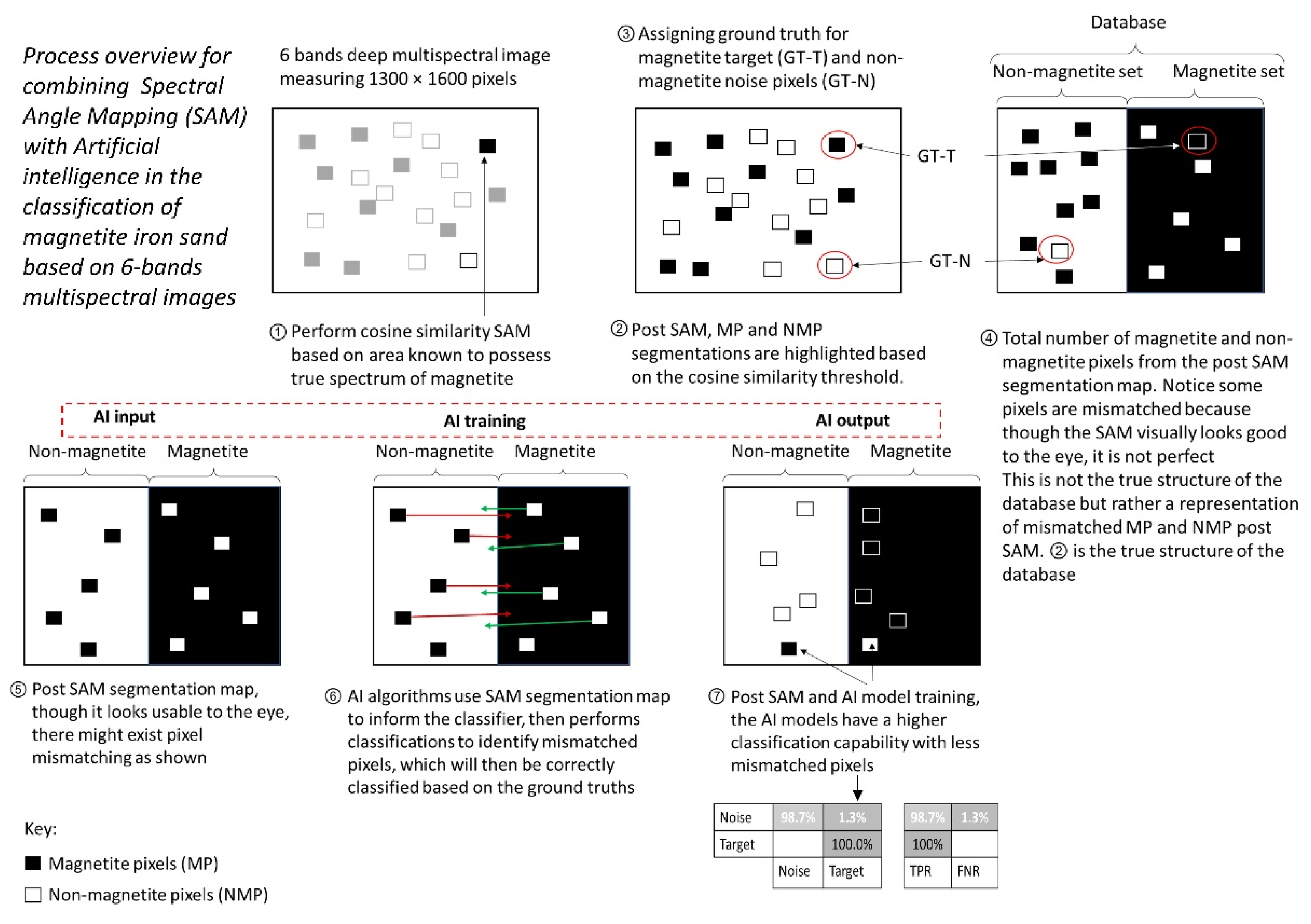
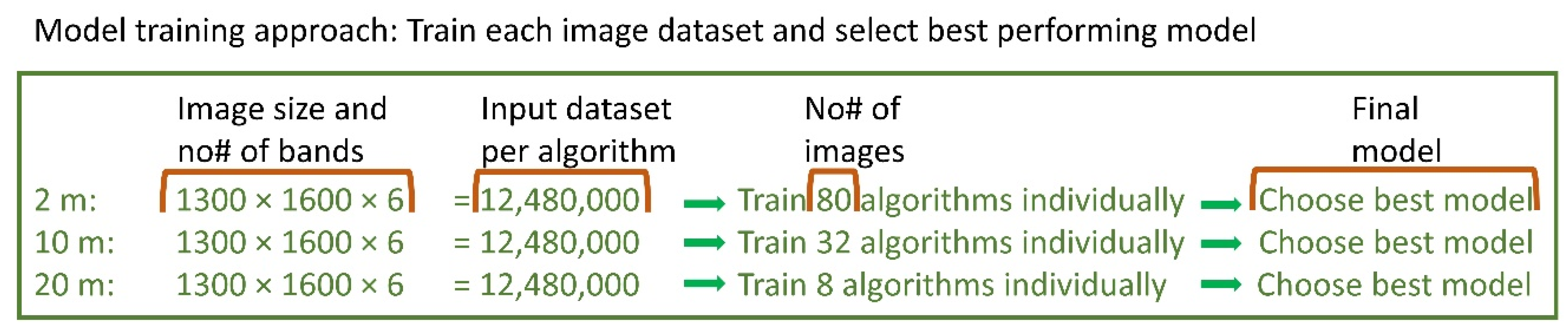
2. Methodological Strategies for SAM and AI Integration

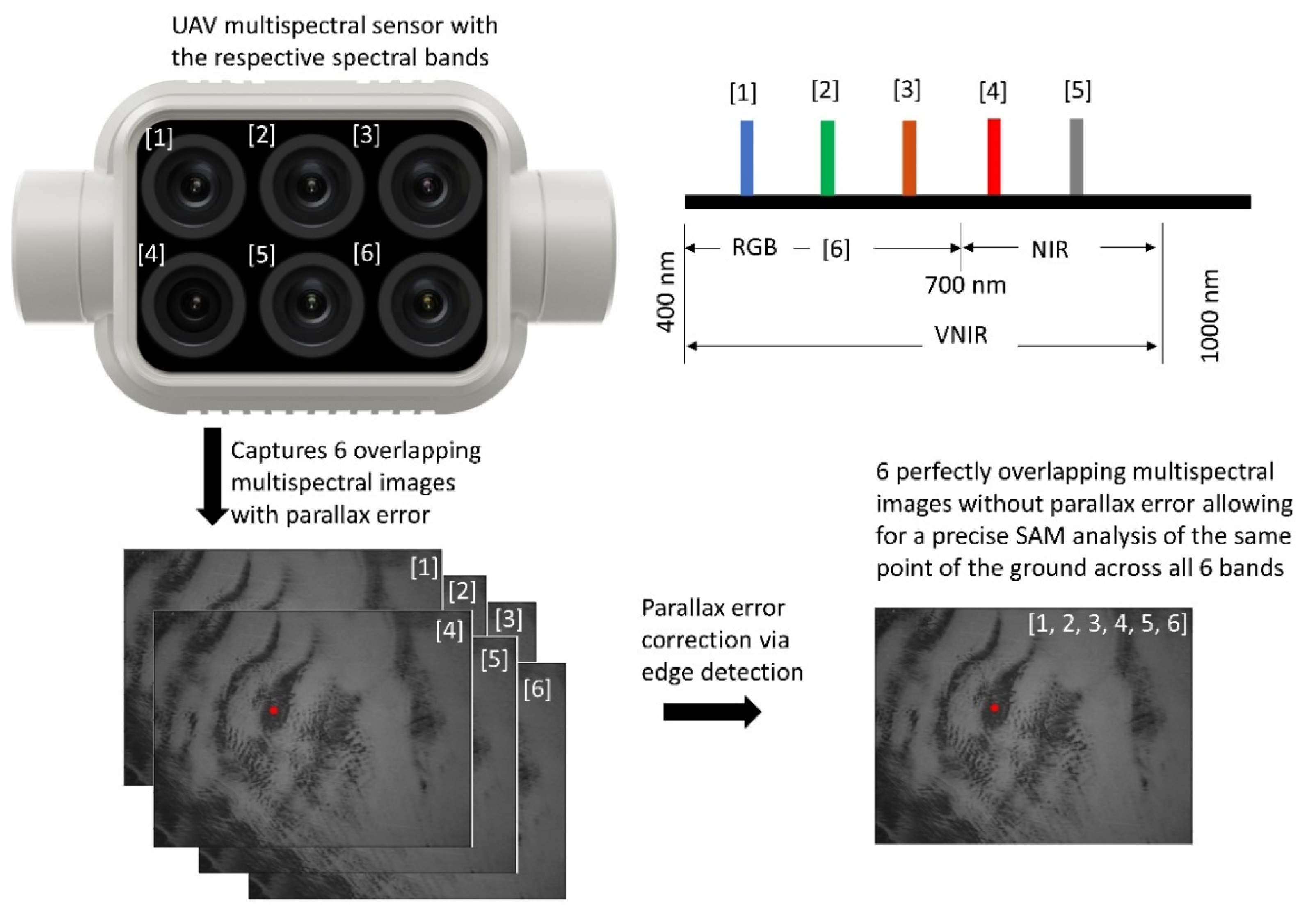
2.1. Combination of UAV Drone Technology with Multispectral Imaging

Air borne drone technology has evolved over the years, with recent developments catering for specialized industrial applications. The protection of human life, as sites can be assessed from a remote area, is one of the major advantages of UAV drone technology [3,22]. In addition, camera-mounted drones aid in real time assessments of sites via visual feed. This footage can be in the form of real, false or pre-processed colours which are meant to represent a certain occurrence understood by the operator [4].
It is supposed that hyperspectral imaging is perhaps one of the best methods by which rocks and minerals can be inferred through their spectral characteristics [5]. However, van de Meer et al. [7] have been able to achieve high classification accuracy outputs in similar rock identification problems via multispectral imaging. Motivated by the demonstrated multispectral capabilities this paper employs a DJI P4 Multispectral camera mounted UAV drone (manufactured by Da-Jiang Innovations, Shenzhen, China) released in September 2019 (Figure 2). To achieve centimeter-level position accuracy, the drone has a real time kinematics (RTK) module attached to it. In addition, the six cameras are 1/2.9-inch (complementary metal oxide semiconductor) CMOS sensors, all at 2 megapixels with a global shutter, on a 3-axis stabilized gimbal to ensure accurate multispectral image capturing at spatial resolutions as high as 0.1 cm/pixel. The spectral sensor specifications are as follows: Blue: 450 nm ± 16 nm, Green: 560 nm ± 16 nm, Red: 650 nm ± 16 nm, Red Edge: 730 nm ± 16 nm, Near Infrared: 840 nm ± 26 nm, which are all captured as TIFF image files. The drone moreover boasts a 62.7° field of view, a net weight of 468 g and an RBG camera which facilitates the extraction of magnetite iron sand spectral information in the visible light spectral range of 400–700 nm as a JPG image. These attributes subsequently make the system effective in a wide range of electromagnetic spectra within the visible-near-infrared range (VNIR) with a total of 6 multispectral bands.
The UAV drone flight elevation plan was set to 3 different variations so as to explore the effect of ground resolution, proximity to the subject, and the ease of flying. From examining these attributes, it would be easier to find the optimal elevation from where magnetite iron sand identification can be performed effectively. The 3 UAV flight elevations measured from the camera sensor to the subject were 2 m, 10 m and 20 m. The drone was moreover programmed such that the aerial multispectral imaging procedure is automatically performed at intervals that ensured an equal amount of area (30 m × 90 m) was captured by the end of each flight mission. In principle, this meant that more multispectral images were to be captured at 2 m with a smaller spatial area per image, followed by 10 m, and the least number of images being captured at 20 m with a relatively larger spatial area. The drone was flown over the 30 m × 90 m area in order to pre-program the flight plan. This flight setting procedure ensures the drone flies within the desired area, direction and elevation before allowing it to perform all these maneuvers autonomously without human intervention.

2.2. Parallax Error Correction

Since there is a small distance between the 6 spectral sensors of the drone, parallax error always needs to be corrected for. This ensures that all sensors are aimed at the same image scene depending on the UAV flight height. At low altitudes, the parallax error is significantly higher relative to higher flight altitudes [23]. There are several methods such as Hough transform and least-squares techniques amongst others which can be applied to perform this task aimed at interpolating the images into perfectly overlapping images [23,24]. However, according to Laurence [24], the edge detection method performs well as it takes into account the individual pixels within each of the 6 multispectral images to be overlapped. It calculates the centers of gravity, and automatically nullifies the differences in position, thereby creating a perfect overlay of images, hence the application of this method in this study [24].
It should be noted however, that in order to assume a perfect overlay, each of the 6 images loses a small part of their edges. The lower the UAV elevation, the more data are lost relative to higher flight elevations. The data loss depends on the distance from the drone sensor to the subject, as well as the distance between sensors within the drone, and so, parallax error always needs to be corrected. Though a small percentage of data is lost per image during parallax correction, this is not the case when considering the study area as a whole. The reason for this is that the UAV flight missions were set up such that each captured image slightly overlaps those around it. This, in principle, ensures zero data loss within the 30 m × 90 m study area, with only the image regions outside the study area experiencing data loss.

2.3. A Scrutiny of SAM Analysis

Based on a number of vegetation criteria, Mohajane et al. [4] have employed several indexes in an attempt to perform rapid field vegetation classification. These included the intensity of certain vegetation colours and moisture content via SAM. Zhang and Li [8] have used the same principle in employing SAM as an index to classify lithology. Weyermann et al. [11] define SAM as a physically based spectral classification that uses an n-dimensional angle to match pixels to reference spectra (Figure 3). The algorithm determines the spectral similarity between spectra by deducing the angle between them, treating them as vectors in a space with dimensionality equal to the number of bands [17], which in this study is 6 bands. This technique, when used on calibrated reflectance data as done in this study, is relatively insensitive to illumination and albedo effects [16]. For this reason, SAM is highly applicable in multitudes of real life field observations, hence the motivation to employ this technique in this study. In short, SAM compares the angle between the endmember spectrum vector and each pixel vector in the n-dimensional space. Narrow angles represent closer matches to the reference spectrum [8]. Pixel data further away from the specified maximum angle threshold in radians are not classified as the reference spectrum of what is sought after, which in this study is magnetite iron sand. Figure 3 illustrates the principle of SAM analysis via cosine similarity.
The drone is linked to a tablet held by the operator on the ground, it receives captured data allowing for on-site SAM analysis, aiding in the identification of magnetite iron sands. Though best performed in the field, this operation can be performed in laboratory analytics. To perform SAM, each captured multispectral image is imported into a SAM operation algorithm such as python. Thereafter, the user pinpoints the area of significance, which in this case was any area within the multispectral image scene known to be occupied by magnetite iron sand. Lastly, the algorithm performs a cosine similarity calculation for every pixel in each image scene to determine whether or not there are similarities between the reference and subsequent subjects [11]. To determine the cosine similarity threshold, Equation (1) is used.
a = cos 1 ( t   ×   t 0 t   ×   t 0 )
where a is the threshold for variables related to the reference, t0 is the reference spectrum, and t is the subject’s true spectrum.
Having successfully stacked the 6 bands TIFF and JPG qualitative images, as well as performing SAM analysis, the images are then converted to csv format. This data conversion provides quantitative values pertaining to magnetite iron sand, and non-magnetite beach sand spectral characteristics, across the 6 multispectral bands. This data structure is useful in training AI algorithms.

2.4. Benefits of Employing AI Methods in Magnetite Identification

In order to determine regions of an image where magnetite iron sands exist post SAM analysis, ML and DL models are an upheld method by which this task can be performed quantitatively [15]. This step involves pre-processing the data before training the AI algorithms. Pre-processing is important as it cleans the data and makes it easier for the algorithms to interpret it; for this study, the pre-processing step involved the extraction of the SAM segmentation maps per image. This simply means magnetite and non-magnetite post SAM spectral variables, given their cosine similarity thresholds, are assigned labels so as to take advantage of supervised AI algorithms. Hence, this process is referred to as image segmentation, and is simply defined as the labelling of each pixel in an image scene [15]. Pixels within and outside the threshold are assigned magnetite and non-magnetite labels, respectively.
Since SAM is mostly a visual interpretation, ground truthing is needed in order to employ AI algorithms. For this reason, the SAM segmentation map is extracted together with two ground truths for magnetite and non-magnetite pixels. Ground truths are image pixels known to be 100% occupied by magnetite and non-magnetite pixels per image. Since each image is 6 bands deep, the result is a total of 12 ground truths. Ground truth for magnetite is defined as the target, whereas non-magnetite ground truth is defined as noise.
Labelled datasets guide and allow algorithms to take advantage of both the global and local structures of the data, which in turn results in quicker and more direct classifications [10]. This in essence means that for each image, the csv file contains labelled pixels for both magnetite iron sands (together with target ground truth), as well as non-magnetite beach sand (together with noise ground truth). Using this data as input, the algorithms are subsequently trained and outputs pertaining to the classification capabilities of the models in deducing magnetite iron sands and non-magnetite beach sand are presented.

2.4.1. How Machine Learning Algorithms Operate

DL is a subset of ML in the broader subject of AI [10]. Though these algorithms are useful in multitudes of data-related tasks such as the classification problem being investigated in this study, they differ in several ways. In order to infer the top performing model at each UAV flight height, both ML and DL AI algorithms are trained.
ML algorithms are mathematical engines of AI, which means these algorithms attribute their classification abilities to perceived mathematical relationships present within the data [19]. In simple terms, ML algorithms try to fit the data within a particular pattern, which can be described using mathematical functions. Since these algorithms are relatively easy to employ, several ML algorithms were trained with regard to the ground truths for target and noise pixel variables. These algorithms were Decision Trees (often abbreviated as Trees) and Ensemble algorithms.
Decision Tree algorithms were employed as they are non-parametric supervised learning methods, used for classification where the goal is to make predictions by learning simple piecewise constant approximation decision rules from data features [25]. Therefore, deeper decision rules are referred to as fine, whereas shallow and less complex decision rules are referred to as course.
In addition to Trees, Ensemble algorithms were employed in the form of Bagged Trees, Subspace K-nearest neighbour (KNN) and Random Undersampling (RUS) Boosted Tress. Bagging is essentially an approach to layering different algorithms [26]. The Subspace KNN on the other hand relies on a stochastic process that randomly selects a number of components of the given feature vector such that when a test sample is compared to a reference, only the selected features have nonzero variables [26]. Lastly, the RUS Boosted Tress model is very useful in alleviating the problem of class balancing when some classes of training data have far fewer observations than others [27]. The RUS Boosted Tress models are fit and added to the ensemble sequentially such that each subsequent model increasingly attempts to correct misclassified predictions of the preceding model [26,27]. These algorithms were employed as they are able to substantially improve prediction performance of learning algorithms in the presence of non-informative features in data. For this reason, Ensemble algorithms are generally referred to as a combination of multiple classifiers.
In summary, both Trees and Ensemble algorithms are highly useful in performing binary and multi-class classifications; consequently, these algorithms were thought of as best fitting for the data structure and research question posed by this study. Post training, the top performing models were examined in terms of classification performances demonstrated at each of the 3 flight elevations based on post SAM and ground truthing procedures.

2.4.2. How Deep Learning Algorithms Operate

DL algorithms, are far more sophisticated in their architecture compared to ML algorithms [10]. They are complex and multilayered, and are built to allow data to pass through information processing layers (like a human brain neurons) in highly connected ways; the result is a non-linear transformation of data which cannot be described by a mathematical function [10,18,19]. It does however take a large amount of data compared to ML to train DL algorithms in order to attain high accuracy output models [19]. For this study, a one dimensional (1D) Convolution Neural Network (CNN) is employed. This type of CNN was applied as it is known to be highly capable in classifying imagery and waveform data [6], which coincides with the data structure presented in this study.

3. Experimental and Analytical Results

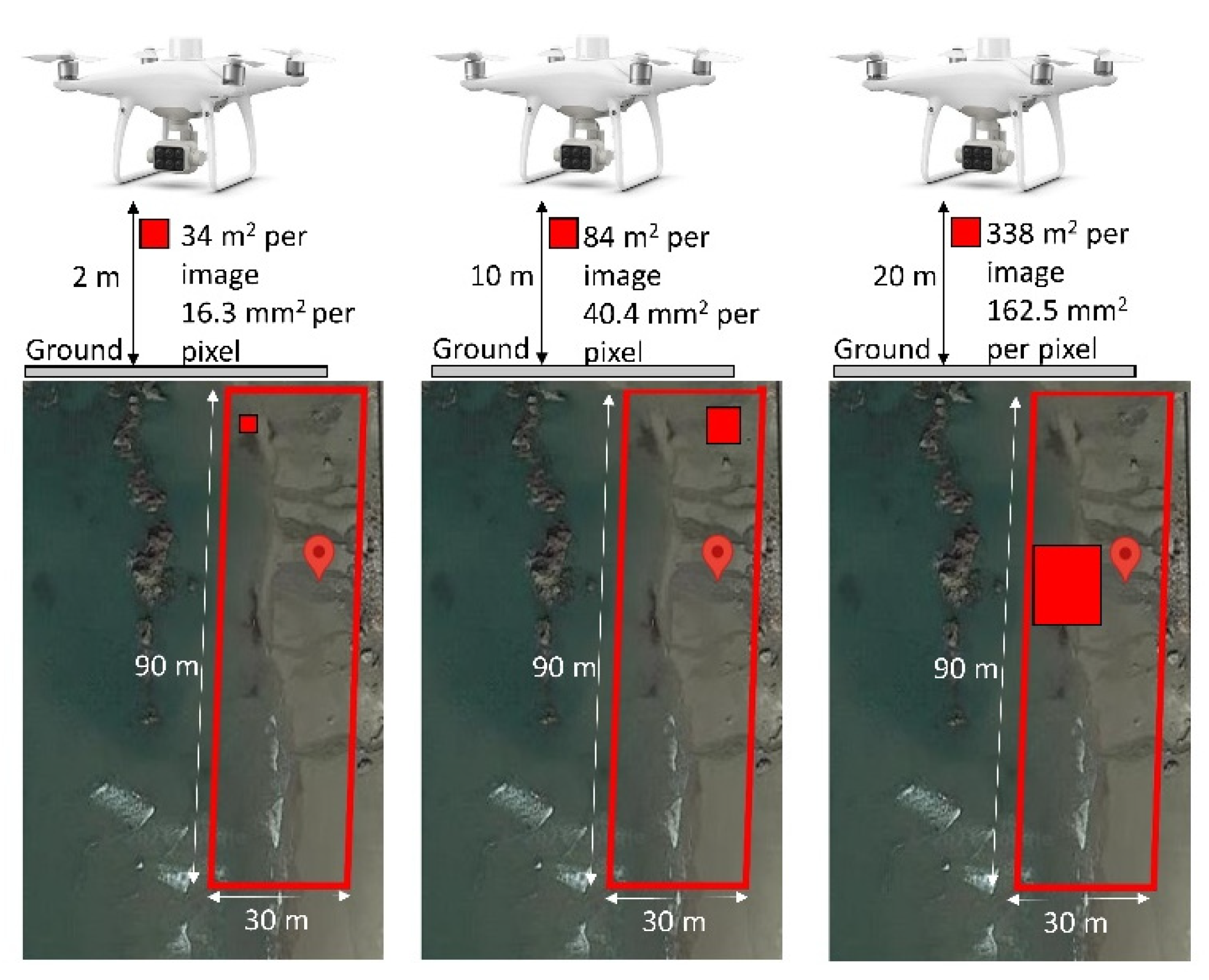
3.1. UAV Drone Field Analytics

From the flight history logs at the different UAV flight elevations, 80, 32 and 8 multispectral images at 2 m, 10 m and 20 m, respectively were captured (Table 1). The number of images is governed by the flight heights, as well as the 62.7° UAV field of view. From the number of images captured, the spatial resolution at each elevation can thus be resolved as shown in Figure 4. Given that each spectral image measures 1300 pixels × 1600 pixels, at 2 m, 10 m and 20 m, the spatial resolutions were 34 m2, 84 m2 and 338 m2, respectively, each multiplied to cover the 2700 m2 study area. Hence, it can be said that the higher the flight elevation, the lower the spatial resolution, the opposite being true at lower flight elevations.
Moreover, based on Figure 4 and Table 1 post flight logs, it has been demonstrated that greater flight elevations allow for a wider area to be captured at a given time. This disregards the need to operate the UAV drone at close proximities to the subject where larger spatial coverage is required. This is a great advantage as it saves time, uses less power, and requires less computational resources to process the numerous multispectral images. Though Table 1 demonstrates the implications of flying at the three different elevations, it does not communicate outputs pertaining to the actual identification of magnetite. This is a task meant for the SAM analysis and AI.

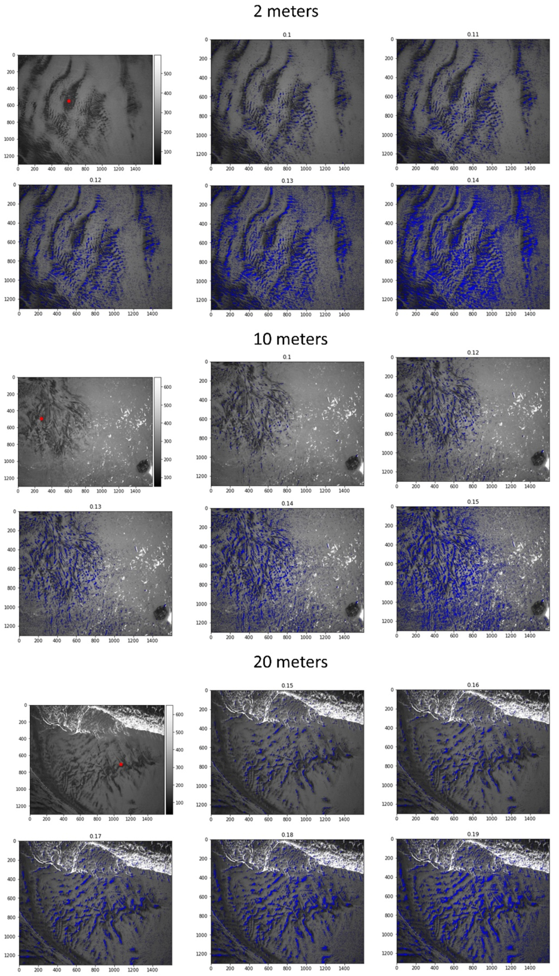
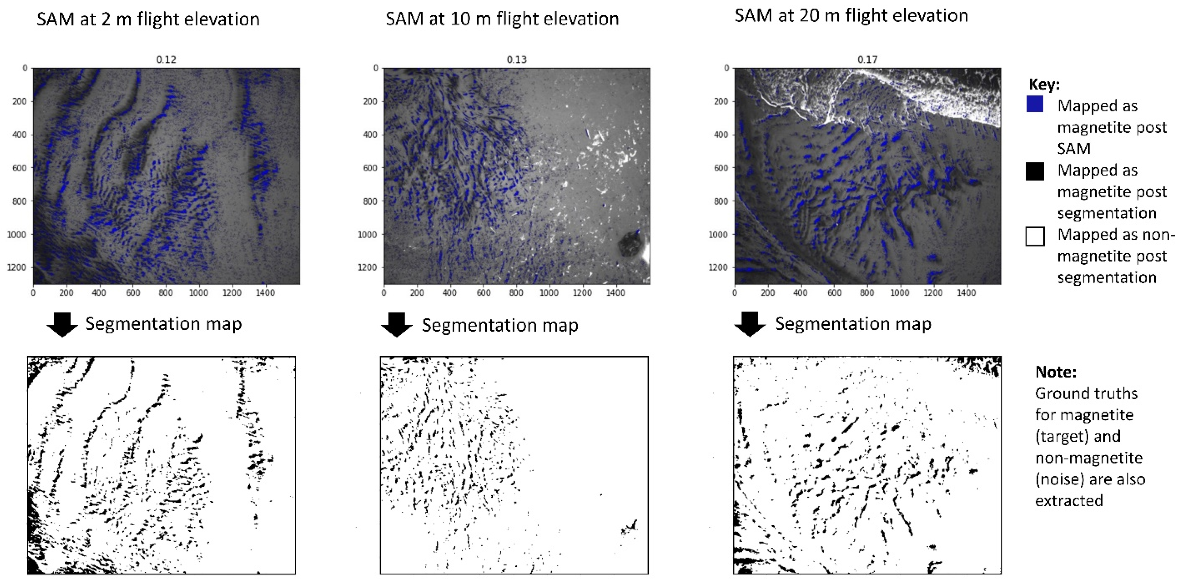
3.2. SAM Analysis Outputs

From the three UAV flight elevations, multispectral images were analyzed and the results show that by varying the reference cosine similarity threshold values, a precise mapping of the area can be attained. By altering their threshold values, Shafri et al. [17] too were able to attain better subject separation. It is clear to see that the SAM analysis performed well across all the three UAV flight elevations from visual analysis of Figure 5. When the threshold value is small, the mask too becomes small, resulting in less of the targeted magnetite iron sands being identified. This in turn means none of the non-magnetite pixels become misidentified. However, where the threshold is larger, more magnetite iron sand pixels are identified. As a result, non-magnetite pixels too are likely to be misidentified as magnetite. This means that one has to manually adjust the threshold such that the mask flawlessly covers the magnetite pixels only.
Based on Figure 5, the best SAM cosine similarity threshold values from visual interpretation were found to be 0.12, 0.13 and 0.17 for 2 m, 10 m and 20 m UAV flight elevations, respectively. From these results, it can hence be said that distance from the sensor to the subject affects the nature of the SAM analysis masks, given that SAM values required alteration for each flight elevation. In summary, at lower UAV drone altitudes, a lower threshold was necessary to identify magnetite iron sands, whereas the opposite was correct at higher UAV drone altitudes. Parallax error was accounted for as previously described in Section 2.2 due to the multispectral sensors being located on different positions on the multispectral camera (Figure 2). This in turn results in a perfect overlay of all six multispectral images at each UAV flight elevation.
Additionally, with larger threshold values, more noise is introduced [16]. This noise is usually caused by mini-ripples and shadows. The SAM analysis is tricked by these ripples into assuming there is resemblance in image pixel characteristics between the actual reference subject and those expressed by ripples and shadows [16]. Even though a visual interpretation of the SAM mask maps seems somewhat instinctive, it can still be argued that this method provides valuable information pertaining to the location of a specific subject such as the magnetite iron sands. There is a plethora of applications within the mining industry where application of this UAV drone coupled with SAM analysis has the potential to be employed. Examples include resource exploration, resource mapping, resource estimation, mine site monitoring, and ore processing amongst others, where quick and accurate separation of rocks and/or minerals is frequently undertaken.

3.3. Application of AI Methods in Magnetite Spectral Classification Post SAM

AI algorithms are a trusted technique by which human error can be eliminated in an objective analysis of data [15], this in turn removes subjectivity pertaining to the visual interpretation of SAM segmentation maps. For each segmentation map, pixels within the 0.12, 0.13 and 0.17 cosine similarity thresholds for the 2 m, 10 m and 20 m flight elevations, respectively, are labelled as magnetite. The rest of the pixel data that are outside the thresholds for each flight elevation are labelled as non-magnetite.
Figure 6 and Figure 7 are representations of how the segmentation maps were extracted via SAM (shown as binarized images for easy visualization), hence creating the labelled segmentation maps across six spectral bands. Thereafter, regions within each image known to be occupied by magnetite iron sand and non-magnetite beach sand are pinpointed so as to act as target and noise ground truths, respectively (Figure 7).
Using the quantitative labelled segmentation maps as demonstrated in Figure 6 and Figure 7, input datasets containing within them magnetite and non-magnetite six bands deep ground truths are ready to be employed in the training and testing of supervised ML and DL algorithms. The output variables are predicted or classified from the training database [10]. This means that algorithms use the ground truths and labelled segmentation maps to try and learn some patterns in the data during training, so as to implement these learnt patterns to the testing dataset [19]. This therefore provides results in relation to the learnt patterns (Figure 7).
At 2 m flight elevation, the total dataset size was 998,400,000, derived from the product of image sizes (1300 × 1600), the number of multispectral bands (6), and the number of captured images (80). At 10 m flight elevation, the total dataset size was 399,360,000, derived from the product of image sizes (1300 × 1600), the number of multispectral bands (6), and the number of captured images (32). Lastly, at 20 m flight elevation, the total dataset size was 99,840,000, derived from the product of image sizes (1300 × 1600), the number of multispectral bands (6), and the number of captured images (8).
These dataset sizes were, however, too large to run using the computational resources employed in this study (32 GB memory, Intel i7-8750H CPU @ 2.2 GHz processor, NVIDIA GeForce GTX 1060 graphics, Windows 10, 64 bits operating system). To counter this, Figure 8 demonstrates our AI training approach. At 2 m flight elevation, the input dataset size used to train each algorithm was 12,480,000, derived from the product of image sizes (1300 × 1600), and the number of multispectral bands (6). Since 80 of such datasets exist, 80 algorithms were trained, and the best performing model from the rest was chosen as the most viable. The same approach was applied at 10 m and 20 m flight elevations, the difference being the number of times (32 times and 8 times, respectively) training was performed, this number corresponding to the number of images captured. With this approach, all image datasets can still participate in the training of the various algorithms, the training times are quicker, and it requires less computational resources.

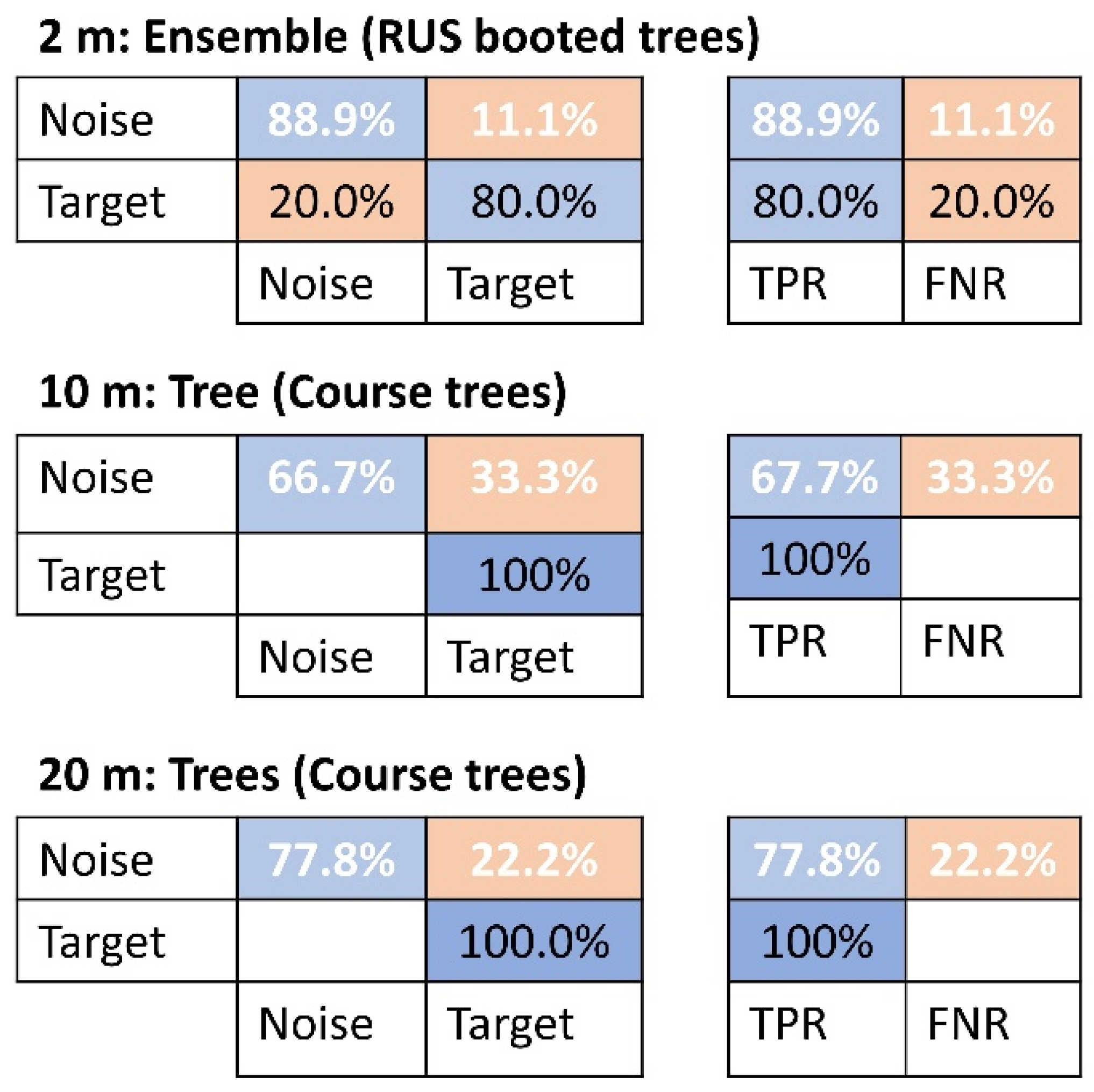
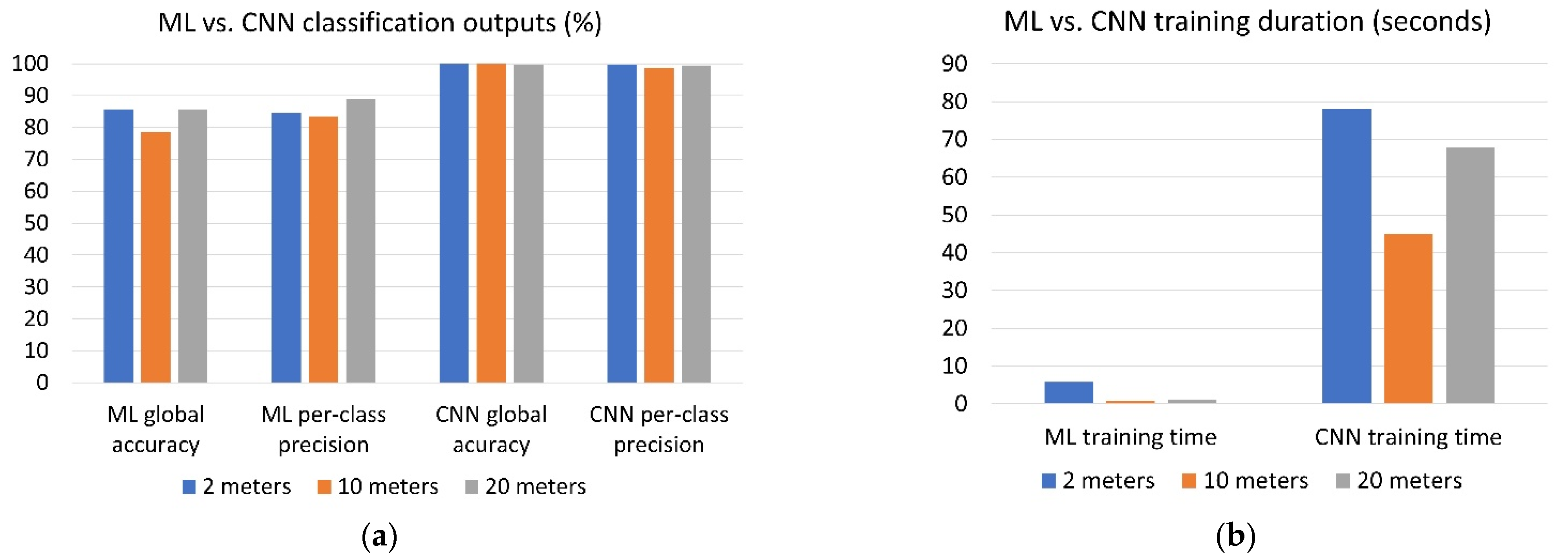
3.3.1. Classification via Machine Learning Models

The input dataset sizes for training and testing variables for each of the ML algorithms stood at 12,480,000 (from Figure 8) for each of the three flight elevation heights. Moreover, a 5-fold-cross-validation was used at all times in order to ensure that every observation (2,496,000 × 5) from the original dataset (12,480,000) has the chance of appearing in training and test sets. Therefore, this method generally results in a less biased model compared to other validation methods [10].
By using the MATLAB R2020b (manufactured by MathWorks, Natick, MA, USA) classification learner Machine Learning toolbox, multiple ML algorithms were evaluated. Classification performances were presented in terms of global accuracy, average per-class precision, and time taken to train the algorithm. These features are said to be amongst the most significant classification evaluation criteria [15]. These outputs, except time taken to train the models, moreover govern industrial applicability, and the overall viability of a model in solving tasks at hand [6]. A compilation of the top three performing ML models for the three multispectral UAV drone flight elevations post SAM and ground truthing are shown in Table 2. The differences in classification capabilities based on flight elevations are demonstrated quantitatively. Global accuracy is defined as the validation accuracy acquired post model training. Average per-class precision refers to the discrete magnetite iron sands (target) and the non-magnetite sands (noise) classification score averages in testing the models. Lastly, training time refers to time taken to train the models to classify the datasets based on the existence or absence of magnetite iron sand. These performance variables are important in comparing the different ML as well as DL models given their intended application.
At 2 m UAV flight elevation, Table 2 results dictate that the best performing model was Ensemble (RUS Boosted Trees). This model acquired a global accuracy of 85.7%, per-class precision of 84.5%, and a training time of 5.8 s. At 10 m UAV flight elevation, the Tree (Course-tree) model performed the best. This model acquired a global accuracy of 78.7%, per-class precision of 83.4%, and a training time of 1 s. Lastly, 20 m UAV flight elevation, the Tree (Course-tree) model performed the best. This model acquired the best outputs in terms of a global accuracy of 85.7%, per-class precision of 88.9%, and a training time of 1 s.
The differences in accuracies acquired and elapsed times when training the ML models for the three UAV flight elevations can, moreover, be appreciated based on the results compiled in Table 2. The reason being, this confirms the initial hypothesis which stated that with the proposed automatic magnetite iron sand identification system, rapid run times and good accuracies are potentially attainable. This is, of course, without compromise to the intrinsic differences in the multispectral characteristics of magnetite iron sands and the surrounding non-magnetite beach sand.
Figure 9 presents two performance metrics used to further assess the viability of the best performing ML models for the three UAV flight elevations. The first is True Positive Rates (TPR), this refers to the probability that an actual positive will test positive (Equation (2)). The second is False Negative Rates (FNR), which are defined as the probability that a true positive will be misclassified by the test (Equation (3)). These two variables are highly viable in assessing the capability of the ML as well as DL models in classifying magnetite iron sands. At 2 m, the ML model has an 80% TPR, which may not seem satisfactory considering that target data should ideally have a 100% target return. This means that 20% of the target pixels were misclassified as noise, suggesting that the model at 2 m did not perform well at discerning magnetite iron sand pixels from the rest of the non-target pixels. In essence, this means that operating and collecting data at this elevation may not be the best practice. At 10 m, the target has a 100% TPR, signifying that the target pixels were correctly classified; this moreover suggests that the target output did not include any noise. At 20 m UAV flight elevation, the same assessment can be made, suggesting that these flight elevations are the most viable out of the three. At 20 m however, the model has a higher noise TRP of 77.8% compared to the 67.7% at 10 m. Consequently, this suggests that the Tree (Course–tree) model at 20 m performed better at discerning the targeted magnetite iron sand data compared to the other two UAV flight elevation model outputs.
One more assessment that can be drawn from the Figure 9 confusion matrix is the average per-class precisions of 84.5%, 83.4% and 88.9% at 2 m, 10 m and 20 m flight elevations, respectively; at 20 m, the model continues to perform better. It can thus be said that the best classification ML model for this magnetite iron sands identification problem is Tree (Course tress) at 20 m.
True Positive Rates (TPR):
TPR = 100 ( TP TP   +   FN )
False Negative Rates (FNR):
FNR = 100 ( FN TP   +   FN )
where FN is false negatives and TP is true positives.

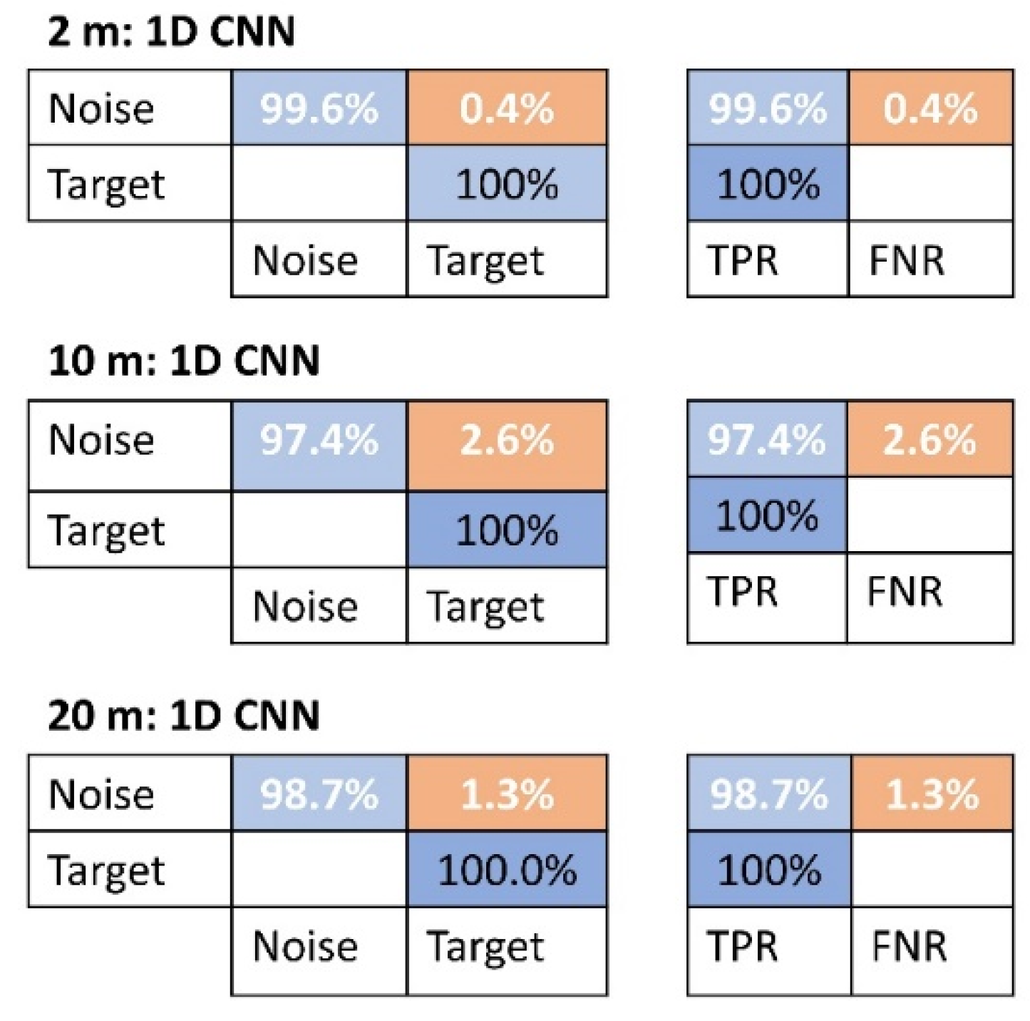
3.3.2. Classification via Deep Learning CNN

A convolution applies a filter over the multispectral data per band. Unlike with visual imagery data with height and width, the filters in a one dimensional CNN exhibit a 1D (spectral intensity) architecture instead of 2D as with normal visual images, hence the motivation to employ this type of CNN in this study as the datasets contain 6-bands deep spectral intensity data that require a 1D data processing method.
The input dataset sizes for training and testing variables for each of the algorithms stood at 12,480,000 (from Figure 8) for each of the three flight elevations prior to obtaining the highest performing model. However, to train the 1D CNN, the spectral data were pre-processed in the following ratios: 70% (9,736,000) designated to training, 15% (1,872,000) validation and the remaining 15% (1,872,000) to testing. Moreover, all models were trained with Adam optimizer, which is said to have a best accuracy in enhancing CNN abilities in classification [19]. A learning rate of 0.001, a batch size of 128, and 25 epochs were also employed. As with ML, the 1D CNN training processes were conducted using the MATLAB 2020b deep learning toolbox with model selection at each flight elevation governed by global accuracy, average per class precision, and time taken to train each 1D CNN algorithm.
At 2 m, 10 m and 20 m flight elevations, 80, 32 and 8 algorithms were trained and one model from the multitudes of trained models was selected. The same procedure was performed in training the ML models. Table 3 is a compilation of the best performing models at each of the three flight elevations. Results from the DL 1D CNN models in Table 3 show that the global accuracies as well as the average per-class precisions have an average of 99.8% and 99.3%, respectively. Moreover, based on global accuracy, the 1D CNN performs the same at 2 m and 10 m at 99.9%, followed by 20 m at 99.7%. However, the trend changes in considering the average per-class precisions where the best performing model is the 1 D CNN at 2 m (99.8%), followed by 20 m (99.4%) and 10 m (98.7%). Lastly, at 2 m, the 1D CNN takes a longer time to train (78 s) compared to the 1D CNNs at 10 m (45 s) and 20 m (68 s); this could suggest that the longer the training time, the higher the average per-class precision for this DL classification problem.
To further assess the viability of the best performing 1D CNN models for the three flight elevations, Figure 10 presents TPR and FNR performance metrics (Equations (2) and (3)). At 2 m, 10 m and 20 m, the 1D CNN models have a 100% TPR for magnetite iron sand (target). This suggests that the models are highly capable of deducing magnetite iron sands from the combination of magnetite iron sands (target) and non-magnetite beach sand (noise). On the other hand, the 1D CNN models attained a 99.6%, 97.4% and 98.7% TPR for non-magnetite beach sand (noise) at 2 m, 10 m and 20 m, respectively, which is considerably high. This suggests that the models are all highly effective at separating magnetite iron sand spectra from non-magnetite beach sand spectra from within the multispectral image scenes.

4. Discussion

In a study by Gholami et al. [28], they applied independent component analysis (ICA) in remote sensing data processing based on satellite data to map an area and attained good results. However, differences between their method and ours are as follows; with the ICA method, they reduced the dimensionality of spectral bands from six bands to two bands. However, researchers mention that higher dimensionalities are relatively superior in deducing materials as they retain the original data structure [5,6,7,8,9]. Hence, our study applied SAM, which retains the full six bands data structure. In addition, our methodology employs a UAV drone, which allows for collection of variables, as well as higher spatial resolution data. For example, at 2 m flight elevation, our spatial resolution is 0.4 cm/pixel, as opposed to their fixed satellite resolution of 30 m/pixel. Considering our 30 m × 90 m study area, their spatial resolution is rather inadequate. Lastly, we employ supervised DL 1D CNN classification algorithms which are known to be state of the art in imagery data classification problems. As pointed out by Sharma and Sharma [10], supervised learning algorithms are superior to unsupervised ML methods such as ICA, especially in cases where the output variables (magnetite or non-magnetite) are known, as is the case in this study.
Based on this study’s findings, it was realised that the SAM cosine similarity thresholds require slight adjustments relevant for each UAV flight elevation. With increase in elevation from 2 m, 10 m to 20 m, these thresholds vary from 0.12, 0.13 to 0.17, respectively. Though these SAM cosine similarities vary, the ability of the SAM in differentiating the targeted magnetite iron sand from non-magnetite beach sand remains relatively unchanged from visual analysis. This is demonstrated by the masks at each flight elevation which seem to flawlessly overlap the sought after magnetite iron sands (Figure 5), as well as the high ground truths-supported AI classification capabilities. With respect to the UAV drone post flight logs and the typical size of surface mines, it would be in the best interest of engineers to perform mineral identification practices at higher elevations such as 20 m. The reason being, the UAV is not as challenged in terms of power consumption, elapsed capturing time, number of images to capture, and area coverage, as at lower elevations (Table 1).
Figure 11 is a summarized comparison between the ML and DL CNN model classification capabilities as well as the length of time required to train each model. Based on global accuracies, the CNN models perform better than the ML models across all three flight elevations. With ML, the attained global accuracies were 85.7%, 78.6% and 85.7% at 2 m, 10 m and 20 m flight elevations, whilst with the CNN, attained global accuracies were 99.9%, 99.9%, 99.7%, respectively. A look into the attained per-class precisions shows that with the ML models, 84.5%, 83.4%, and 89. A total of 9% classification capabilities were attained at 2 m, 10 m and 20 m flight elevations. These model classification capabilities are different from the 99.8%, 98.7% and 99.4% attained via the CNN at 2 m, 10 m and 20 m, respectively. Therefore, it can be said that based on the global accuracies as well as the per-class precisions (Figure 11a), model capabilities show that the 1D CNNs employed in this study are far superior in classifying the magnetite iron sands, and non-magnetite beach sands, to the ML models.
From Figure 11b, one is able to appreciate the differences in times required to train the AI models. With ML models, training times are shorter (5.8, 0.9 and 1.0 s at 2 m, 10 m and 20 m, respectively) compared to those of the CNN models (78, 45 and 68 s at 2 m, 10 m and 20 m, respectively). Though the ML model training times seem relatively more efficient, the time taken to train a model is not what governs its industrial applicability. Training duration merely communicates the time it took to turn an algorithm into a model via training.
Lastly, considering the UAV flight logs, as well as the AI model outputs in this study, one can come to the conclusion that the most effective UAV flight elevation is 20 m. At 20 m, one has a larger spatial area coverage, which eliminated the need to capture multitudes of images. Matching these variables with the attained AI model classifications, shows that the best classifier at this UAV flight elevation in identifying magnetite iron sands is the 1D CNN.

5. Conclusions

This study proposed the employment of a 6-bands multispectral UAV drone-mounted camera in the automatic identification of magnetite iron sands at a placer deposit. As an initial step, the UAV drone was flown at three different flight elevations of 2 m, 10 m, and 20 m so as to find the optimum magnetite iron sand identification flight elevation. From the flight time, power consumption and number of spectral images capturing flight logs, 20 m flight elevation was the most viable. This study went on to examine the SAM analysis maps at these three flight elevations. It was found that the SAM cosine similarities could indeed identify the magnetite iron sand target areas at 2 m, 10 m and 20 m at 0.12, 0.13 and 0.17 cosine similarity threshold values, respectively, from the 6 bands multispectral images.
Using the respective cosine similarity thresholds per flight elevation, the paper continued to address the viability of coupling SAM analysis segmentation maps as well as ground truths, with different AI models. It was found that the proposed coupled system did indeed yield industry viable outputs across all flight heights. However, considering all outputs of this study, it was found that the best overall performance ratios were demonstrated at 20 m flight elevation. At this elevation, the UAV drone was able to capture 6-bands multispectral images with a spatial resolution of 338 m2. Furthermore, using the 6-bands multispectral imagery data, a 1D CNN DL model with a global accuracy of 99.7% and a per-class precision of 99.4% was found to be the overall best AI model.
System capabilities with the potential for applicability in the mining industry/sphere have been demonstrated by this study. Said applications include rock and mineral exploration from a remote location; mapping of mine sites via UAV drone technology; the ability to classify rocks and minerals based on their cosine similarities (SAM analysis) to a reference spectrum; the ability to take advantage of multispectral imaging from an elevation and distance of one’s choosing, and lastly, the flexibility of applying objective AI models in the classification of rocks and minerals (as demonstrated with magnetite).

Author Contributions

Conceptualisation, B.B.S. and Y.K.; Data curation, H.T.; Formal analysis, H.I.; Funding acquisition, Y.K. and T.A.; Investigation, B.B.S.; Methodology, B.B.S.; Resources, H.I.; Software, N.O.; Supervision, Y.K.; Validation, Z.B. and E.S.; Visualisation, H.I. and H.T.; Writing—original draft, B.B.S.; Writing—review & editing, Z.B., E.S., T.A. and Y.K. All authors have read and agreed to the published version of the manuscript.

Funding

This work was supported by the Cooperative Research Project Program of the Penta-Ocean Construction Co., Ltd.

Data Availability Statement

Not applicable.

Acknowledgments

‘Inter-University Exchange Project: An Innovative Program for Development of Core Human Resources for Smart Mining to Lead Sustainable Resource Development in Southern Africa’. Part of this work was carried out under the Cooperative Research Project Program of the Penta-Ocean Construction Co., Ltd. JSPS ‘Establishment of Research and Education Hub on Smart Mining for Sustainable Resource Development in Southern African Countries’ (JPJSCCB2018005).

Conflicts of Interest

The authors declare no conflict of interest.

Appendix A

The procedure for coupling SAM with AI algorithms is as follows; At Figure 7 ①, a region within an image that is known to possess magnetite iron sands is pinpointed and used as a reference from which SAM is performed. As Figure 6 and Figure 7 ② show, though a SAM may seem satisfactory from visual observations, it is rarely, if ever, 100% perfect. To overcome this, Figure 7 ③ shows how ground truth pixels are extracted from post SAM segmentation maps. Ground truths are the pixels known to be 100% occupied by magnetite (target) and non-magnetite (noise) pixels. When two (magnetite and non-magnetite) ground truth pixels are extracted from the 6-bands deep spectral images, we end up having a total of 12 ground truths (6 for each material).
By the end of the segmentation (Figure 7 ②), we end up with a given total number of magnetite and non-magnetite pixels per segmented image across 6 spectral bands as shown in Figure 7 ④. Hence, Figure 7 ④ is not the true structure of the image datasets but rather a sum of all pixels thought to be magnetite and non-magnetite post SAM.
Thereafter, the segmentation maps are inserted into AI algorithms together with their target and noise ground truths (Figure 7 ⑤). The AI algorithms then attempt to classify the whole image scene containing the segmentation map based on the pre-defined ground truths for magnetite and non-magnetite pixels. From Figure 7 ⑥, we see the algorithms identifying and reclassifying pixels which may not have been correctly classified/mapped by the SAM in Figure 7 ②. At the end of the AI classification procedure (Figure 7 ⑦), we see that the AI models have better/improved classification capabilities. Though not perfect either as shown by the confusion matrix, the classification capabilities are significantly more viable than pre-AI. In short, the post SAM segmentation maps as well as the ground truths help guide, inform and speed up the decision making process of the supervised AI algorithms in classifying magnetite iron sand and non-magnetite sands.

References

  1. Sinaice, B.B.; Takanohashi, Y.; Owada, N.; Utsuki, S.; Hyongdoo, J.; Bagai, Z.; Shemang, E.; Kawamura, Y. Automatic magnetite identification at Placer deposit using multi-spectral camera mounted on UAV and machine learning. In Proceedings of the 5th International Future Mining Conference 2021—AusIMM 2021, Online, 6–8 December 2021; pp. 33–42, ISBN 978-1-922395-02-3. [Google Scholar]
  2. Gaffey, C.; Bhardwaj, A. Applications of Unmanned Aerial Vehicles in Cryosphere: Latest Advances and Prospects. Remote Sens. 2020, 12, 948. [Google Scholar] [CrossRef] [Green Version]
  3. Erbe, H.-H.; Udd, J.E.; Sasiadek, J.Z. Mining Automation. IFAC Proc. Vol. 2004, 37, 299–304. [Google Scholar] [CrossRef]
  4. Mohajane, M.; Essahlaoui, A.; Oudija, F.; El Hafyani, M.; Cláudia Teodoro, A. Mapping Forest Species in the Central Middle Atlas of Morocco (Azrou Forest) through Remote Sensing Techniques. IJGI 2017, 6, 275. [Google Scholar] [CrossRef] [Green Version]
  5. Fox, N.; Parbhakar-Fox, A.; Moltzen, J.; Feig, S.; Goemann, K.; Huntington, J. Applications of Hyperspectral Mineralogy for Geoenvironmental Characterisation. Miner. Eng. 2017, 107, 63–77. [Google Scholar] [CrossRef]
  6. Sinaice, B.B.; Kawamura, Y.; Kim, J.; Okada, N.; Kitahara, I.; Jang, H. Application of Deep Learning Approaches in Igneous Rock Hyperspectral Imaging. In Proceedings of the 28th International Symposium on Mine Planning and Equipment Selection—MPES 2019; Springer Series in Geomechanics and Geoengineering; Topal, E., Ed.; Springer International Publishing: Cham, Switzerland, 2020; pp. 228–235. [Google Scholar] [CrossRef]
  7. van der Meer, F.D.; van der Werff, H.M.A.; van Ruitenbeek, F.J.A.; Hecker, C.A.; Bakker, W.H.; Noomen, M.F.; van der Meijde, M.; Carranza, E.J.M.; de Smeth, J.B.; Woldai, T. Multi- and Hyperspectral Geologic Remote Sensing: A Review. Int. J. Appl. Earth Obs. Geoinf. 2012, 14, 112–128. [Google Scholar] [CrossRef]
  8. Zhang, X.; Li, P. Lithological Mapping from Hyperspectral Data by Improved Use of Spectral Angle Mapper. Int. J. Appl. Earth Obs. Geoinf. 2014, 31, 95–109. [Google Scholar] [CrossRef]
  9. Ganesh, U.K.; Kannan, S.T. Creation of Hyper Spectral Library and Lithological Discrimination of Granite Rocks Using SVCHR -1024: Lab Based Approach. J. Hyperspectral Remote Sens. 2017, 7, 168–177. [Google Scholar]
  10. Sharma, N.; Sharma, R.; Jindal, N. Machine Learning and Deep Learning Applications-A Vision. Glob. Transit. Proc. 2021, 2, 24–28. [Google Scholar] [CrossRef]
  11. Weyermann, J.; Schläpfer, D.; Hueni, A.; Kneubühler, M.; Schaepman, M. Spectral Angle Mapper (SAM) for Anisotropy Class Indexing in Imaging Spectrometry Data. In Proceedings of the Imaging Spectrometry XIV, San Diego, CA, USA, 17 August 2009; p. 74570B. [Google Scholar] [CrossRef] [Green Version]
  12. Hu, H.; Feng, D.-Z.; Chen, Q.-Y. A Novel Dimensionality Reduction Method: Similarity Order Preserving Discriminant Analysis. Signal Process. 2021, 182, 107933. [Google Scholar] [CrossRef]
  13. Rauhala, A.; Tuomela, A.; Davids, C.; Rossi, P. UAV Remote Sensing Surveillance of a Mine Tailings Impoundment in Sub-Arctic Conditions. Remote Sens. 2017, 9, 1318. [Google Scholar] [CrossRef] [Green Version]
  14. Martelet, G.; Gloaguen, E.; Døssing, A.; Lima Simoes da Silva, E.; Linde, J.; Rasmussen, T.M. Airborne/UAV Multisensor Surveys Enhance the Geological Mapping and 3D Model of a Pseudo-Skarn Deposit in Ploumanac’h, French Brittany. Minerals 2021, 11, 1259. [Google Scholar] [CrossRef]
  15. Saha, D.; Annamalai, M. Machine Learning Techniques for Analysis of Hyperspectral Images to Determine Quality of Food Products: A Review. Curr. Res. Food Sci. 2021, 4, 28–44. [Google Scholar] [CrossRef] [PubMed]
  16. Girouard, G.; Bannari, A.; Harti, A.E.; Desrochers, A. Validated Spectral Angle Mapper Algorithm for Geological Mapping: Comparative Study between Quickbird and Landsat-TM. 6. 2014. Available online: https://www.researchgate.net/publication/228799788_Validated_spectral_angle_mapper_algorithm_for_geological_mapping_comparative_study_between_QuickBird_and_Landsat-TM (accessed on 4 July 2021).
  17. Shafri, H.Z.M.; Suhaili, A.; Mansor, S. The Performance of Maximum Likelihood, Spectral Angle Mapper, Neural Network and Decision Tree Classifiers in Hyperspectral Image Analysis. J. Comput. Sci. 2007, 3, 419–423. [Google Scholar] [CrossRef] [Green Version]
  18. den Hartog, D.; Harlaar, J.; Smit, G. The Stumblemeter: Design and Validation of a System That Detects and Classifies Stumbles during Gait. Sensors 2021, 21, 6636. [Google Scholar] [CrossRef] [PubMed]
  19. Chauhan, D.; Anyanwu, E.; Goes, J.; Besser, S.A.; Anand, S.; Madduri, R.; Getty, N.; Kelle, S.; Kawaji, K.; Mor-Avi, V.; et al. Comparison of Machine Learning and Deep Learning for View Identification from Cardiac Magnetic Resonance Images. Clin. Imaging 2022, 82, 121–126. [Google Scholar] [CrossRef] [PubMed]
  20. Kobayashi, S.; Ikuta, K.; Sugimoto, R.; Honda, H.; Yamada, M.; Tominaga, O.; Shoji, J.; Taniguchi, M. Estimation of submarine groundwater discharge and its impact on the nutrient environment at Kamaiso beach, Yamagata, Japan. Nippon. Suisan Gakkaishi 2019, 85, 30–39. [Google Scholar] [CrossRef] [Green Version]
  21. Nguyen, H.H.; Carter, A.; Hoang, L.V.; Vu, S.T. Provenance, Routing and Weathering History of Heavy Minerals from Coastal Placer Deposits of Southern Vietnam. Sediment. Geol. 2018, 373, 228–238. [Google Scholar] [CrossRef] [Green Version]
  22. Beretta, F.; Rodrigues, A.L.; Peroni, R.L.; Costa, J.F.C.L. Automated Lithological Classification Using UAV and Machine Learning on an Open Cast Mine. Appl. Earth Sci. 2019, 128, 79–88. [Google Scholar] [CrossRef]
  23. Ono, M. Parallax Error Correction Techniques by Image Matching for ASTER/SWIR Band-to-Band Registration. In Proceedings of the Platforms and System, Rome, Italy, 9 January 1995; pp. 18–27. [Google Scholar] [CrossRef]
  24. Laurence, S.J. On Tracking the Motion of Rigid Bodies through Edge Detection and Least-Squares Fitting. Exp. Fluids 2012, 52, 387–401. [Google Scholar] [CrossRef] [Green Version]
  25. Singh Kushwah, J.; Kumar, A.; Patel, S.; Soni, R.; Gawande, A.; Gupta, S. Comparative Study of Regressor and Classifier with Decision Tree Using Modern Tools. Mater. Today Proc. 2021, S2214785321076574. [Google Scholar] [CrossRef]
  26. Mohammadi, M.; Rezaei, J. Ensemble Ranking: Aggregation of Rankings Produced by Different Multi-Criteria Decision-Making Methods. Omega 2020, 96, 102254. [Google Scholar] [CrossRef]
  27. Haixiang, G.; Yijing, L.; Shang, J.; Mingyun, G.; Yuanyue, H.; Bing, G. Learning from Class-Imbalanced Data: Review of Methods and Applications. Expert Syst. Appl. 2017, 73, 220–239. [Google Scholar] [CrossRef]
  28. Gholami, R.; Moradzadeh, A.; Yousefi, M. Assessing the Performance of Independent Component Analysis in Remote Sensing Data Processing. J. Indian Soc. Remote Sens. 2012, 40, 577–588. [Google Scholar] [CrossRef]
Figure 1. Study area map showing Kamaiso magnetite iron sand placer deposits. Red polygon denotes the 30 m by 90 m study area within which the UAV drone shown was flown. Map acquired from: Google maps (2021).
Minerals 12 00268 g001
Figure 2. The 6-bands multispectral sensor with a 62.7° field of view; (1) Blue: 450 nm ± 16 nm, (2) Green: 560 nm ± 16 nm, (3) Red: 650 nm ± 16 nm, (4) Red Edge: 730 nm ± 16 nm, (5) Near Infrared: 840 nm ± 26 nm and (6) RGB camera: 400–700 nm represent the multispectral sensor capabilities. Images captured are corrected for parallax error via an edge detection method. The red point is the reference area from which magnetite iron sands are known to exist.
Minerals 12 00268 g002
Figure 3. Schematic diagram showing the principle of spectral angle mapping via cosine similarity. Reference spectrum is the sought after target. Angle a is the cosine similarity threshold between a reference and a true spectrum.
Minerals 12 00268 g003
Figure 4. Illustration of the difference spatial resolutions of each image, attained from capturing multispectral images at 2 m, 10 m, and 20 m flight elevations.
Minerals 12 00268 g004
Figure 5. SAM analysis at 2 m, 10 m and 20 m UAV drone elevations at different reference spectral thresholds. The red points represent the user-selected reference point known to be magnetite (pre-SAM), whilst the blue overlay represent areas within the threshold limit thought to be magnetite (post SAM cosine similarity). The best threshold cosine similarities are 0.12, 0.13 and 0.17 at 2 m, 10 m and 20 m, respectively. The x and y axis represent the size of each captured multispectral image. The bar on the right of each first image represents the variation in spectral intensities present in each captured image. Reprinted with permission from ref. [1]. 2021 AusIMM [1] (p. 38).
Minerals 12 00268 g005
Figure 6. Extraction of 6-bands deep segmentation maps (binazized for easier visual representation) used to create a magnetite iron sand database. Noise refers to non-magnetite pixels. Segmentation maps at each UAV flight elevation are based on the 0.12, 0.13 and 0.17 cosine similarity thresholds at 2 m, 10 m and 20 m. This process is summarized in step ② of Figure 7, as well as Appendix A.
Minerals 12 00268 g006
Figure 7. Proposed process overview with emphasis on how data extracted from spectral angle mapping cosine similarities is segmented, assigned ground truths, and used in training artificially intelligent algorithms in the classification of magnetite iron sand. Appendix A has extended explanations on this procedure.
Minerals 12 00268 g007
Figure 8. Input dataset sizes used to train the machine learning and deep learning algorithms as well as selection of the best performing model at each UAV flight elevation.
Minerals 12 00268 g008
Figure 9. Machine learning confusion matrices from Ensemble (RUS Boosted Trees) at 2 m UAV drone elevation, Tree (Course-tree) at 10 m UAV drone elevation, and Tree (Course-tree) at 20 m UAV drone. Reprinted with permission from ref. [1]. 2021 AusIMM [1] (p. 40).
Minerals 12 00268 g009
Figure 10. Deep learning one dimensional convolution neural network confusion matrices at 2 m, 10 m and 20 m UAV drone elevation.
Minerals 12 00268 g010
Figure 11. Best performing machine learning vs. deep learning classification models based on 0.12, 0.13 and 0.17 SAM cosine similarity thresholds at 2 m, 10 m and 20 m, respectively: (a) Comparisons based on global accuracy and pre-class precision; (b) Comparisons based on model training durations.
Minerals 12 00268 g011
Table 1. Multispectral UAV drone post flight records from investigations carried out at three different flight elevations. Reprinted with permission from ref. [1]. 2021 AusIMM [1] (p. 37).
UAV Drone Flight Elevation Number of Images CapturedFlight Time (Minutes:
Seconds)
Spatial Area Coverage
(m2)
Battery Power Consumed during Mission (%)
2 m8021: 323469
10 m328: 238429
20 m82: 083387
Table 2. Top 3 machine learning classification model comparisons at 2 m, 10 m and 20 m UAV flight elevations based on 0.12, 0.13 and 0.17 SAM cosine similarity thresholds, respectively. Reprinted with permission from ref. [1]. 2021 AusIMM [1] (p. 40).
UAV Drone Flight ElevationMachine Learning ModelGlobal Accuracy (%)Average Per-Class Precision (%)Training Time
(Seconds)
2 mEnsemble (Bagged Trees)78.683.48.4
Ensemble (Subspace KNN)71.477.88.1
Ensemble (RUS Boosted Trees)85.784.55.8
10 mTree (Fine-tree)78.683.41.5
Tree (Medium-tree)78.683.41.0
Tree (Course-tree)78.683.40.9
20 mTree (Fine-tree)85.788.91.9
Tree (Medium-tree)85.788.91.2
Tree (Course-tree)85.788.91.0
Table 3. Deep learning one dimensional convolution neural network classification model comparisons at 2 m, 10 m and 20 m UAV flight elevations based 0.12, 0.13 and 0.17 SAM cosine similarity thresholds, respectively.
Flight HeightGlobal Accuracy (%)Average Per-Class Precision (%)Training Time
(Seconds)
2 m99.9%99.8%78
10 m99.9%98.7%45
20 m99.7%99.4%68
Publisher’s Note: MDPI stays neutral with regard to jurisdictional claims in published maps and institutional affiliations.

