1. Introduction
The traveling salesman problem (TSP) is one of the most well-known combinational optimization problems studied in the operation research literature. It consists of determining a tour that starts and ends at a given base node after visiting a set of nodes exactly once while minimizing the total distance [
1]. Solving the TSP problem is crucial because it belongs to the class of non-polynomial (NP)-complete. In this class of problems, no polynomial–time algorithm has been discovered. If someone finds an efficient TSP algorithm, it can be extended to other NP-complete class issues. Unfortunately, to date, no one has been able to do it. The TSP is divided into two categories, symmetric and asymmetric, based on the distance between any two nodes. In asymmetric TSP (ATSP), the distance from one node to another is different from the inverse distance, and in symmetric TSP (STSP), this distance is the same. As previously mentioned, the TSP consists of determining a minimum-distance circuit passing through each vertex once and only once. Such a circuit is known as a tour or Hamiltonian circuit (or cycle) [
2].
A large number of exact algorithms have been proposed to solve the TSP problem. In addition to exact algorithms, some heuristic algorithms are used to provide high-quality solutions, but not necessarily optimal. The importance of identifying effective heuristics to solve large-scale TSP problems prompted the ‘8th DIMACS Implementation Challenge, organized by Johnson et al. [
3] and solely dedicated to TSP algorithms [
4]. Lin and Kernighan’s heuristic algorithm appears so far to be the most effective in terms of solution quality, particularly with the variant proposed by Helsgaun (2000) [
5]. Potvin (1996) [
6] proposed a genetic algorithm to the TSP, and Aarts et al. (1988) [
7] analyzed the TSP problem with the simulated annealing algorithm [
8]. All of the traveling salesman problems have a similar structure by one difference. The basic model is as follows:
subject to Equation (2)
In this formulation, Equation (1) is the objective function that minimizes the total distance and is distance or weight of arc (i,j), Equations (2) and (3) are the assignment constraint, which ensures that each node is visited and left exactly once, and Equations (4) and (5) indicate that is a binary variable and equals to 1 if arc (i,j) participates in the tours.
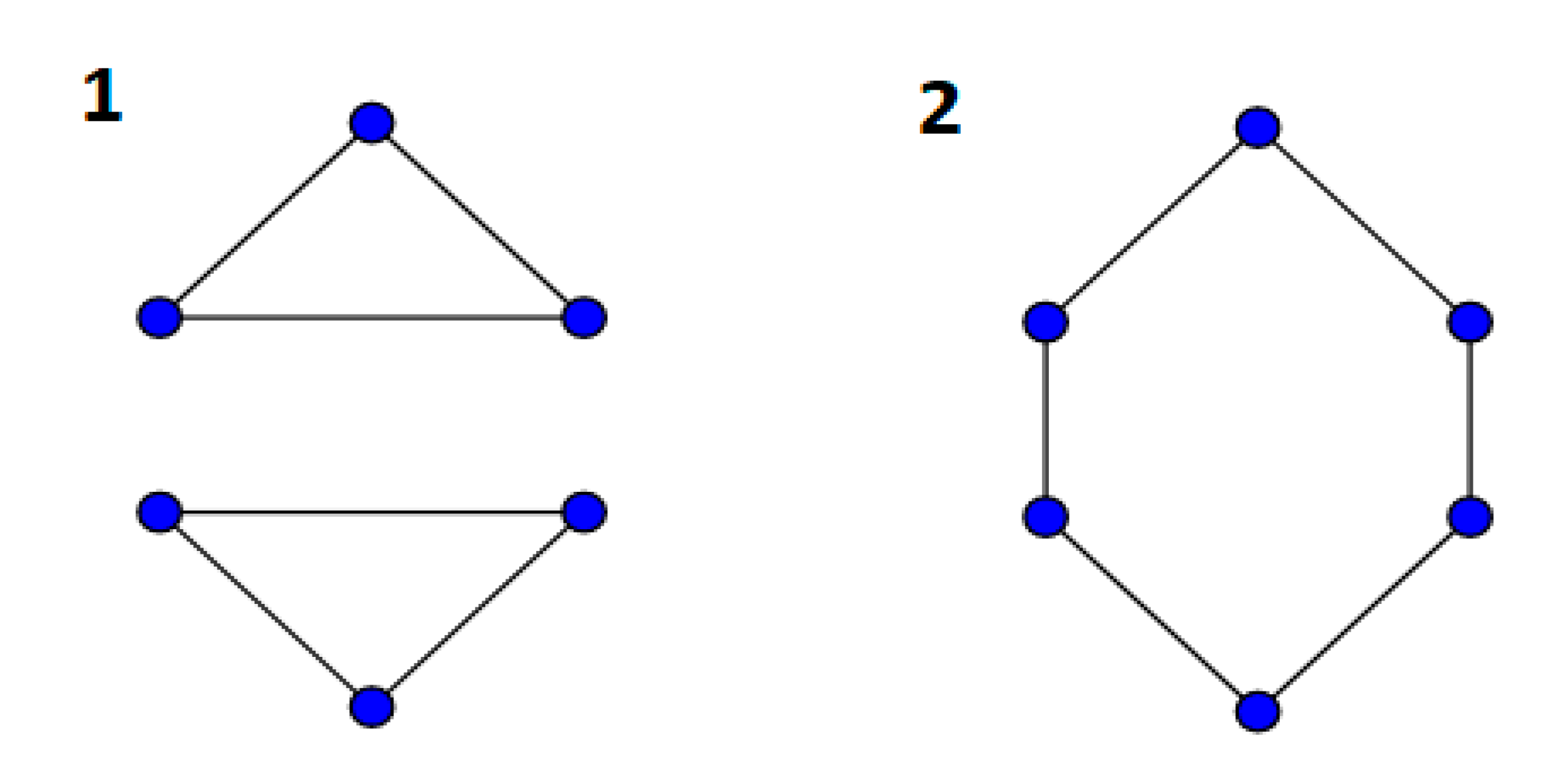
The basic model that is mentioned above is not complete because it does not support the Hamiltonian circuit. Suppose there are six nodes and a traveler wants to visit all of them, he can do this in the two ways shown in
Figure 1:
In the above graphs (1 and 2), all of the nodes are visited, but in (1), we do not have a Hamiltonian circuit. This figure indicates that the basic formulation is not complete and should use a constraint that omits graph (1). For that, researchers add a constraint to the basic formulation for eliminating these sub-tours. Researchers have proposed many constraints for sub-tour breaking, but it is not clear which one is better. Therefore, in this research, an attempt has been made to compare the three methods most used in articles. This study used a multi-criteria decision-making method for the evaluation and comparison of these three constraints. Since the purpose of the research is to survey the three formulations, it is proposed to use the simultaneous evaluation of criteria and alternatives (SECA) method for decision making and ranking. One of this method’s properties is that it does not need experts’ opinions for weighting criteria. The SECA method can compute weights of criteria by mathematical methods.
2. Description of Three Sub-Tour Elimination Constraints (SECs)
2.1. The Danzig–Fulkerson–Johnson (DFJ) Formulation
Danzig, Fulkerson, and Johnson proposed the first integer linear programming (ILP) formulation in 1954 as an SEC [
9]. The DFJ constraints are
In each subset Q, sub-tours are prevented, ensuring that the number of arcs selected in Q is smaller than the number of Q nodes [
10].
yij is a binary variable and is equal to 1 when the nodes of
i,
j are visited. Q is a set of vertices whose cardinalities are between 3 and
n − 1 because two nodes cannot take a tour, and the minimum number for making a tour is 3.
2.2. The Miller–Tucker–Zemlin (MTZ) Formulation
The earliest known extended formulation of the TSP was proposed by Miller in 1960 [
11]. It was initially proposed for a vehicle routing problem (VRP), where each route’s number of vertices is limited [
12]. The VRP can be simply defined as the problem of designing least-cost delivery routes from a depot to a set of geographically scattered customers, subject to side constraints. This problem is central to distribution management and must be routinely solved by carriers. In practice, several variants of the problem exist because of the diversity of operating rules and constraints encountered in real-life applications [
13]. The capacitated vehicle routing problem (CVRP) is one of the variants of the VRP. The CVRP consists, in its basic version, of designing a set of minimum cost-routes for several identical vehicles having a fixed capacity to serve a set of customers with known demands [
14]. The MTZ constraints are
In this formulation
and
are integer variables that define the order of vertices visited on a tour.
yij is a binary variable and is equal to 1 when the nodes of
i,
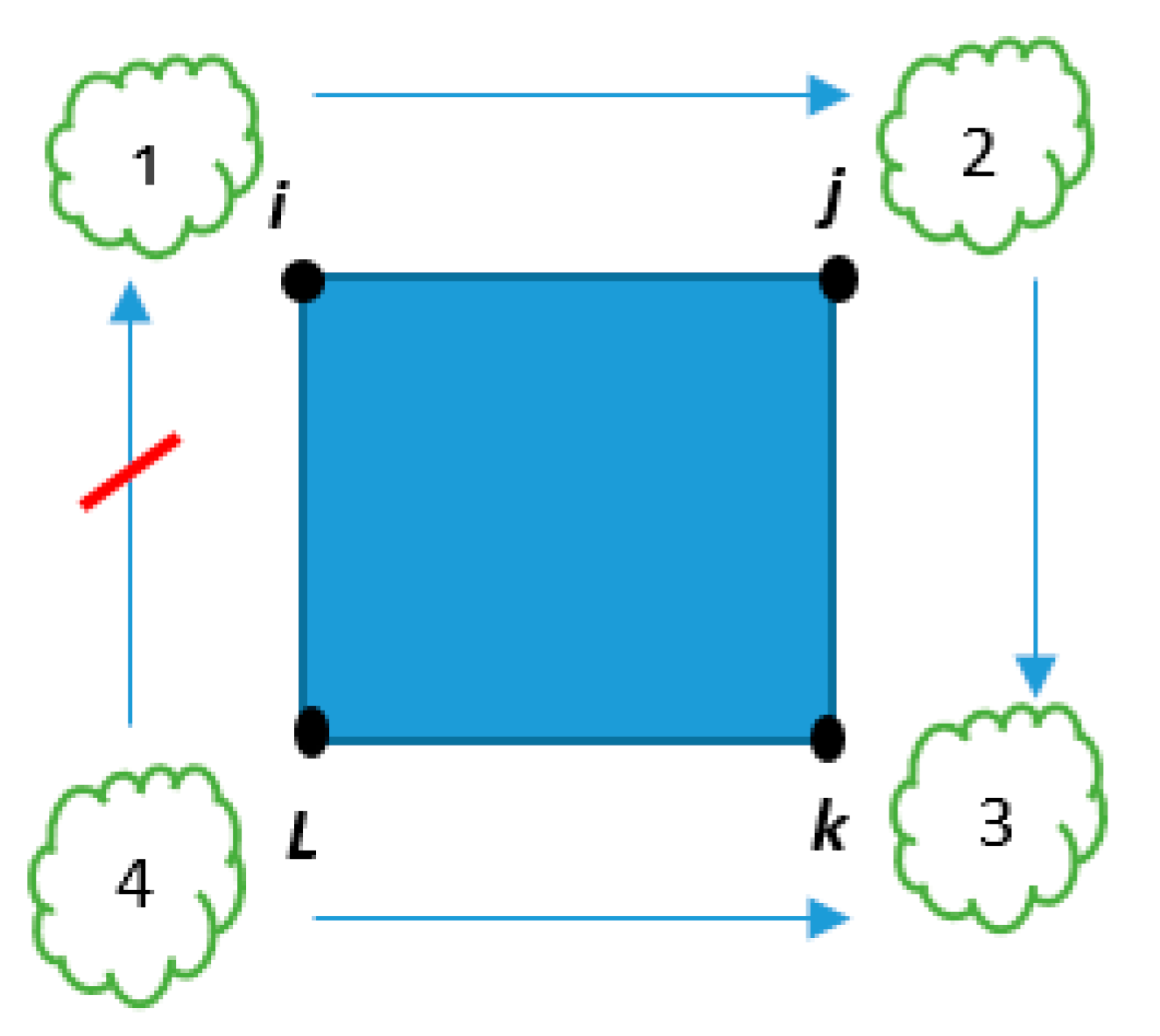
j are visited. Constraint acts on the basis of node labeling. This means each node receives a number label, and these numbers should be sequential.
Figure 2 shows that each number is greater than the previous one except in the last one (1 is not greater than 4). This simple rule helps prevent the TSP from making arc
i,
l and eliminate taking a tour.
2.3. The Gavish–Graves (GG) Formulation
A large class of extended ATSP formulations is known as commodity flow formulations, where the additional variables represent commodity flows through the arcs and satisfy additional flow conservation constraints. These models belong to three classes: single-commodity flow (SCF), two-commodity flow (TCF), and multi-commodity flow (MCF) formulations. The earliest SCF formulation is due to Gavish and Graves. The additional continuous non-negative variables
zij describe a single commodity’s flow vertex 1 from every other vertex [
12]. The GG [
15] formulation for a single commodity problem that has sub-tour elimination constraints in it is
In this formulation, z is a positive variable. yij is a binary variable and is equal to 1 when the nodes of i,j are visited. Constraint (7) ensures that the flow variable (Zij) exists between nodes with one unit following. Constraint (8) assures that a flow is possible when the nodes are connected (yij = 1).
3. Research Gap
As indicated, there are many SECs of the TSP formulation in literature. Researchers prefer using one of them based on their previous experiences. Consequently, if someone enters this field, they do not know which one is more related to their work. Sometimes new researchers use one method that is not proper for their research. For example, when the number of nodes increases, using the DFJ method is not suitable because it is an exponential growth of constraints that make it complicated for the software to achieve a result. Nevertheless, some researchers use the DFJ method in problems with a high number of nodes. However, there has been no research attending to all aspects or details. Some researchers select SECs just for their lower constraints or variables. Others work on the relaxation to get better answers, which are nearer to the optimum. So far, researchers have not considered all related criteria that impact the selection of SECs. This study attempted to cover the criteria that have the most impact on the selection of SECs. Consider someone who wants to use SECs for sub-tour elimination. He faces DFJ and realizes that DFJ gets an answer nearer to an optimum value, but it has many constraints and needs more time for running, and for the exponential growth of constraints, it needs a more powerful computer. With these properties of DFJ, is its selection suitable or not? The MTZ method gets results comparable to an optimum value, but it generates integer variables and incredibly increases the problem’s complexity. The GG method does not get a result near the optimum value, but it has fewer constraints than DFJ and has no integer variable. With these properties, which one of them is better than the others?
Accordingly, it was decided to convey three SECs used more than others in research and determine which of them is better and related to our work.
4. Methodology
The core of operations research is the development of approaches for optimal decision making. A prominent class of such problems is multi-criteria decision making (MCDM) [
16]. There are many MCDM methods in the literature. These approaches are classified according to the type of data (deterministic, stochastic, and fuzzy) and to the number of decision-makers (single, group). In the decision-making process, usually three steps are followed for numerical analysis of alternatives:
- (1)
Specifying the relevant criteria and alternatives
- (2)
Assigning numerical measures to the criteria under the impact of alternatives
- (3)
Ranking each alternative
According to these steps, various methods have been proposed. In continuation, some prevalent MCDM methods introduced recently are explained.
The best–worst method (BWM) was proposed by Rezaee (2015). In this method, decision-makers first determine some decision criteria and then identify the best (most desirable) and the worst (least desirable). These criteria (best and worst) are compared to other criteria (pairwise comparison). A maximin problem is then formulated and solved to determine the weights of different criteria [
17].
With the aid of some aggregation strategies, Yazdani et al. (2018) introduced a new method, which is a combined compromise decision-making algorithm [
18]. They called it CoCoSo, which is an abbreviation of combined compromise solution. This method is used to compromise normalization, which was proposed by Zeleny (1973) [
19]. The CoCoSo weight of alternatives is determined by three equations achieved by the aggregated multiplication rule.
Stevic et al. (2019) proposed a new method: measurement alternatives and ranking according to compromise solution (MARCOS). This method is based on defining the relationship between alternatives and reference values (ideal and anti-ideal alternatives). Based on the defined relationships, the utility functions of alternatives are determined and compromise ranking is made in relation to ideal and anti-ideal solutions. Decision preferences are defined on the basis of utility functions. Utility functions represent the position of an alternative concerning an ideal and anti-ideal solution. The best alternative is the one that is closest to the ideal and at the same time furthest from the anti-ideal reference point [
20].
This study uses the SECA method for decision making and ranking [
21]. One of the reasons for selecting this method is that experts, like most other methods, do not need to allocate weights of criteria. This study compares three mathematical constraints and does not need expert opinion for scoring the criteria. It recommends two reference points (the standard deviation and correlation) and then minimizes the deviation of criteria weights from the reference point. The score of each alternative and the weight of each criterion are determined with software. The SECA model is multi-objective non-linear programming, which uses some techniques for optimization, and the formulation is equal to
subject to
where
denotes the performance value of
i-th alternative on
j criterion and
wj is the weight of each unknown criterion. Moreover,
, each vector elements’ standard deviation
, shows the degree of conflict between
j-th criterion and other criteria. In addition,
, a small positive parameter, is equal to 10
−3 as a lower bound for criteria weights. The coefficient
β is used for minimizing deviation from reference points. In the source paper, it is mentioned that when the values of
β are greater than 3 (
), the performance of alternatives is more stable. Therefore,
β is taken to be 3 in this study.
Si shows the overall performance score of each alternative.
The SECA method also is used in the evaluation of sustainable manufacturing strategies. In this decision model, SECA is combined with a weighted aggregated sum product assessment (WASPAS) [
22].
5. Selection of Related Criteria by Reviewing Articles
Defining related criteria is the essence of using the MCDM methods. The MCDM methods indeed evaluate multiple conflicting criteria, but this does not mean that the criteria are not related to the issue. So, selecting proper criteria is an essential step in decision making. There are two ways to choose criteria. One way is to review some articles and convey on them to select the right criteria. The other way is to consult with experts and use what they opt for. This study used both methods for selecting related criteria. Further research that deals with this issue was undertaken, and a summary is provided in the following content.
ATSP formulations are shown in
Table 1, and the order of their variables and constraints will be determined like this [
12]:
To complete their comparative study, they tested the LP relaxation of these models. The result of this comparison shows that DFJ is better than GG, and GG is better than MTZ, which means the result of LP relaxation of the DFJ model is closer to the optimal value. Their results are similar to Wong’s research [
23].
Orman and Williams classified models into four groups: conventional (C), sequential (S), flow-based (F), and time-staged (T) [
24]. They extracted the following information:
- (1)
DFJ is located in the C group, and the combination of the base model with this sub-tour elimination has constraints and n(n − 1) 0–1 variables, because the exponential number of constraints cannot solve this practically.
- (2)
MTZ is located in the S group, and the combination of the base model with this sub-tour elimination has constraints, n(n − 1) 0–1 variables, and (n − 1) continuous variables.
- (3)
GG is located in the F1 group, and the combination of the base model with this sub-tour elimination has n(n + 2) constraints, n(n − 1) 0–1 variables, and n(n − 1) continues variables.
- (4)
To demonstrate the relative strengths of LP relaxations of these SECs, they provide the following results (
Table 2) for 10 cities’ TSP.
Benhida and Mir [
25] compared DFJ and MTZ sub-tour elimination and declared that the DFJ formulation of the TSP contains
n(
n − 1) variables and
constraints. MTZ contains (
n − 1)(
n + 1) variables and
constraints. To compare this method, they randomly generated 10 complete graphs from 10 to 950 nodes. These nodes were randomly taken between 0 and 99 coordinates. The distances between the nodes are Euclidean distances (d), and they calculated the relaxation value (R) by relaxing the integrality constraints. They reported the results in a table and showed the R values of DFJ and MTZ for 10 to 950 nodes. This final result of the research was that the DFJ relaxation value is better than the MTZ relaxation value, and MTZ is charming because it is easy to implement but gives a low continuous relaxation.
By reviewing the above articles and consulting with experts, six criteria that have a significant impact on the selection of SECs are chosen and listed below:
- (1)
Number of constraints: when this criterion increases, the time to solve increases, too.
- (2)
Number of variables: these criteria affect the solution time.
- (3)
Relaxation value: whatever is closer to an optimum value is better.
- (4)
Number of nodes: it affects solution time and SEC performance.
- (5)
Type of variable: integer variables increase the complexity of a problem.
- (6)
Time in second: the time to find a solution is a significant issue in selecting a method.
6. Computational Results
After defining related criteria, the three sub-tour elimination constraints should be evaluated. In this evaluation, the number of nodes is considered constant in each step of comparison. Optimization software is needed to assess these SECs. This study uses CPLEX 12.8 for coding these three sub-tour eliminations (codes attached in
Appendix A). In this code, we calculated the optimal answer for different nodes with a random distance (rand (10) + rand (200)), and we reported the results in
Table 3. When the number of nodes increases, the difficulty of a problem also increases. In mathematical optimization, relaxation is a modeling strategy. Solving problems by a relaxation variable provided useful information about the original problem. DFJ relaxation gets the best answer from others because it has one type of variable (binary). MTZ gets the worst solution for its two types of variables (integer and binary).
For relaxation in CPLEX, we changed the type of variable to float+ and added a constraint (0 ≤ yij ≤ 1).
7. Using the SECA Method for Ranking Computational Results
With the information in
Table 4, which is achieved by comparing the criteria, it is possible to use the MCDM method. As mentioned before, among the decision-making methods, SECA is selected in this research. Now, in this section, we implement the stages of this method. At first, like other MCDM methods, define a decision matrix for a problem and normalize it. In the decision matrix,
xij denotes the performance value of alternatives (
i) on each criterion column (
j). Use linear normalization for normalizing. In this, the criteria are divided into two sets, beneficial and non-beneficial. Linear normalization formulation is
After normalization, this formulation should be used to calculate the degree of conflict between the criteria.
rjl is the correlation between
j and
l vectors.
After calculating the standard deviation of the elements of each vector (
), we normalize
and
by these formulations:
In our problem, there are three alternatives and five criteria. The score of the nodes should be calculated for the ranking of alternatives. It should be considered that it is not possible to use
xij = 0 in the SECA model. For this reason, the cells that are zero are converted to 1. One may ask why it is allowed to substitute 0 with 1 in the decision matrix. As mentioned above, the minimum amount of
x in SECA method is 1 and cannot use a smaller number. The significant number of nodes (100 and 500) in which there are no criteria values less than 1 are calculated to confirm this research result. In the table given below, gap is the difference between the optimal and the relaxed value, and the less the value, the better and beneficial it is. An example of the decision matrix is used to show the case of Node = 15 in
Table 4.
After implementing the stages for calculating σ and π (the steps are provided in
Appendix B), each alternative’s computing score should be calculated using optimization software. This work used LINGO 11 software for coding the SECA optimization model (exist in
Appendix C). We got the following results for each node (
Table 5). Their ranking is shown in
Table 6.
By looking at the ranking table, we understand that GG is the best method between the three SEC formulations. For testing, the SECA method’s scoring used the website
www.mcdm.app (accessed on 25 December 2020), which has a powerful calculation engine and covers many MCDM methodologies. As seen, the GG method has some features that lead it to the first place. One reason making it better from the MTZ method is the type of variables. GG has no integer variable that increases the complexity of a problem. When the number of nodes increases, the DFJ method’s constraints extend exponentially, and an optimum computing value is more challenging for a computer. As we see in the above tables, when the number of nodes is more significant than 19, typically, personal computers will not be able to compute an optimum value for DFJ and to report the result, because estimating this large volume of calculations, personal computers run out of random access memory (RAM). RAM is short-term storage that holds programs and processes running on a computer. Behinda and Mir calculated the DFJ method for many cities, which is in contrast to the paper’s result. This may occur for several reasons; for example, they might use powerful computers with high RAM (they do not refer to the system’s information). This study uses a usual computer (the system used for this research had an 8 GB RAM and a CPU with seven cores). One of the reasons may be due to the ATSP, because in this type of problem, the route between two cities is different from the return route, and this issue increased the complexity of the solution. Using parallel computing or changing the amount of rand can get an answer for many cities. For these reasons, the codes used in this study are attached in the
Appendix C for readers.
Applegate et al. [
26] decided to solve various TSP instances and constructed a library named TSPLIB. They used DFJ sub-tour elimination. The size of cities ranged from 17 to 85,900. For the largest, of 85,900 nodes, they used 96 workstations for a total of 139 years of CPU time [
8].
8. Conclusions
One of the usual problems for a researcher in using TSP formulation is to select the best sub-tour elimination constraint. As everyone may know, many SEC formulations are presented, but it is not specified which of them is most suited to our work. So, they should be compared to each other to determine which of them is superior. This study analyzes three SECs of the TSP formulation (DFJ, MTZ, and GG), which are used more than others in research. For comparison using MCDM methods, some criteria needed to be introduced. By reviewing research papers, five criteria were concluded: the number of constraints, the number of variables, type of variables, time of solving, and the differences between optimum and relaxed value, and that was the main research gap of the study. These SEC formulations are non-linear. When the number of nodes rises, solving problems with non-linear variables is hard. For this reason, these variables are turned into linear variables, because linear problems are solved quickly. This conversion is named LP relaxation. Therefore, the lower value of the gap is more suitable because the relaxation value is closer to its optimum value. It should be mentioned that the relaxation value gets a lower bound of a problem. Whenever this lower bound is more comparable to an optimum value, the result reaches the optimum by fewer iterations in the optimization software.
This research aimed to analyze the three sub-tour elimination formulations of the ATSP by an MCDM method. This study used the simultaneous evaluation of criteria and alternatives (SECA) method for multiple decision making and ranking the alternatives. The computation of this method shows that GG SEC is better than others. Comparison between DFJ and MTZ does not show a distinct difference, but as shown, the DFJ SEC’s computing is time-consuming because, as the number of nodes increases, the constraints grow exponentially. This particular reason drives us to use MTZ SEC in the ATSP problem, especially when the number of nodes increases.
If we look at
Table 4, we may ask why GG is better than MTZ, while MTZ has fewer variables and constraints and takes less time to solve. To answer this question, it is better said, as mentioned before, that MTZ has a charming face. One of the criteria considered in this study is the type of variables. MTZ generates integer variables, and as we know, these variables increase the complexity of solving. The real traveling salesman problem could not reach the exact answer in polynomial time because this is an NP_hard problem.
Thus, researchers used heuristic methods to obtain an upper bound and relaxation to earn a lower bound for these problems. They know the answer is in this interval. Relaxation of the MTZ constraint should get two types of variables, binary and integer. Most of the times, the relaxation variable is not an integer, and other methods should be used to convert it into an integer, but GG does not have this problem because it has binary and positive variables and gets a relaxation value that is closer to the optimum value. Therefore, the type of variable is a crucial criterion and significantly affects the ranking of alternatives. So, the main reason for this ranking is this criterion. Covering all aspects, this study proposes that GG is the best sub-tour elimination.
Author Contributions
Conceptualization, R.B. and S.H.Z.; methodology, R.B.; software, S.H.Z.; validation, S.H.Z. and R.B.; formal analysis, S.H.Z. and S.M.J.M.A.-e-h.; investigation, R.B.; data curation, R.B.; writing—original draft preparation, R.B. and S.H.Z.; writing—review and editing, R.B. and S.H.Z.; supervision, S.H.Z. and S.M.J.M.A.-e-h.; project administration, S.H.Z.; funding acquisition, S.H.Z. All authors have read and agreed to the published version of the manuscript.
Funding
There is no external fund for this study.
Acknowledgments
The authors acknowledge, with thanks, Danesh Tabatabaee, the master’s student of the Department of Industrial Management Systems and Engineering, Amirkabir University of Technology, for help in software coding.
Conflicts of Interest
There is no conflict of interest.
Appendix A
CPLEX code:| DFJ: |
| //define number of nodes |
| int nbnode=10; // define parameter |
| range nodes=1..nbnode; // define index |
| |
| //c is the distance between nodes |
| float c[i in nodes][j in nodes]=rand(10)+rand(200); |
| |
| //in this section define set and subset |
| range ss = 1..ftoi(round(2^nbnode)); |
| {int} sub [s in ss] = {i | i in 1..nbnode: (s div ftoi(2^(i-1))) mod 2 == 1}; |
| |
| //model |
| dvar boolean y[nodes][nodes]; // y is decision variable |
| which |
| is binary. |
| minimize sum(i,j in nodes)c[i][j]*y[i][j]; //objective function |
| subject |
| to{ //constraints |
| forall (j in nodes) sum(i in nodes)y[i][j]==1; |
| forall (i in nodes) sum(j in nodes)y[i][j]==1; |
| forall (s in ss: 2<card(sub[s])<nbnode) sum(i, j in sub[s]) y[i][j] <= card(sub[s])-1; |
| |
| } |
| MTZ: |
| //define number of nodes |
| int nbnode=10; // define parameter |
| range nodes=1..nbnode; // define index |
| |
| //c is the distance between nodes |
| float c[i in nodes][j in nodes]=rand(10)+rand(200); |
| |
| //model |
| dvar boolean y[nodes][nodes]; //y is binary variable |
| dvar int+ u[nodes]; // u is integer variable |
| |
| minimize sum(i,j in nodes)c[i][j]*x[i][j]; //objective function |
| subject |
| to{ //constraints |
| forall (j in nodes) sum(i in nodes)y[i][j]==1; |
| forall (i in nodes) sum(j in nodes)y[i][j]==1; |
| forall (i,j in nodes: j!=1) u[i]-u[j]+nbnode*y[i][j]<=nbnode-1; |
| } |
| GG: |
| //define number of nodes |
| int nbnode=10; // define parameter |
| range nodes=1..nbnode; // define index |
| |
| //c is the distance between nodes |
| float c[i in nodes][j in nodes]=rand(10)+rand(200); |
| |
| |
| //model |
| dvar boolean y[nodes][nodes]; //y is binary variable |
| dvar float+ z[nodes][nodes]; //z is positive variable |
| |
| minimize sum(i,j in nodes)c[i][j]*y[i][j]; //objective function |
| subject |
| to{ //constraints |
| forall (j in nodes) sum(i in nodes)y[i][j]==1; |
| forall (i in nodes) sum(j in nodes)y[i][j]==1; |
| forall (i in nodes: i>=2 ) sum(j in nodes)z[i][j]-sum(j in nodes: j!=1)z[j][i]==1; |
| forall (i,j in nodes: i!=1) z[i][j]<=(nbnode-1)*y[i][j]; |
| |
| } |
Appendix B
Table A1.
Normalized decision matrix.
Table A1.
Normalized decision matrix.
| Normalize | Constraint | Variable | Type | Time | Gap |
|---|
| DFJ | 0.007375 | 1 | 1 | 0.166667 | 1 |
| MTZ | 1 | 0.9375 | 0.0625 | 1 | 0.061463 |
| GG | 0.948819 | 0.517241 | 1 | 1 | 0.699301 |
Table A2.
Standard deviation of criteria.
Table A2.
Standard deviation of criteria.
| STD | 0.456343 | 0.214367 | 0.441942 | 0.392837 | 0.39131 |
|---|
| STD-N | 0.240598 | 0.113021 | 0.233006 | 0.207116 | 0.206311 |
Table A3.
Correlation of criteria.
Table A3.
Correlation of criteria.
| rij | Constraint | Variable | Type | Time | Gap |
|---|
| Constraint | 1 | −0.5622 | −0.53913 | 0.998951 | −0.77613 |
| Variable | −0.56225 | 1 | −0.39336 | −0.59953 | −0.08508 |
| Type | −0.53913 | −0.3933 | 1 | −0.5 | 0.949517 |
| Time | 0.998951 | −0.5995 | −0.5 | 1 | −0.74644 |
| Gap | −0.77613 | −0.0850 | 0.949517 | −0.74644 | 1 |
Table A4.
Calculate π = (1 − rij).
Table A4.
Calculate π = (1 − rij).
| 1 − rij | Constraint | Variable | Type | Time | Gap | Sum Each Row | Πn |
|---|
| Constraint | 0 | 1.562251 | 1.539128 | 0.001049 | 1.77613 | 4.878559 | 0.199069 |
| Variable | 1.56225 | 0 | 1.393365 | 1.599526 | 1.085082 | 5.640223 | 0.230148 |
| Type | 1.53913 | 1.39336 | 0 | 1.5 | 0.050483 | 4.482973 | 0.182927 |
| Time | 0.001049 | 1.59953 | 1.5 | 0 | 1.746444 | 4.847023 | 0.197782 |
| Gap | 1.77613 | 1.08508 | 0.050483 | 1.74644 | 0 | 4.658133 | 0.190074 |
Table A5.
Ranking of alternatives by score.
Table A5.
Ranking of alternatives by score.
| | SCORE | Ranking |
|---|
| DFJ | 0.6233 | 2 |
| MTZ | 0.6233 | 2 |
| GG | 0.8356 | 1 |
Appendix C
| Code of SECA in LINGO 11 for node=15: |
| MODEL: |
| |
| SETS: |
| AL/1..3/:S; #AL is alternatives and s is score |
| CR/1..5/: W,zig,p; # CR is criteria |
| LINK (AL, CR): X; # X denoted the performance value of |
| alternatives on each criterion column |
| ENDSETS |
| |
| #read data from excel file |
| DATA: |
| B=3; #B is beta in the SECA method |
| #zig is the normalization of standard deviation |
| #p is the normalization of sum (1- correlation) of each row |
| X, zig, p=@OLE(‘C:\MATRIX.XLSX’,‘DECISION’,‘SIG’,‘PI’); |
| ENDDATA |
| |
| @FOR (AL (I): |
| s(I)=@SUM (CR(J):W(J)*X(I,J)); |
| LA <=S (I); |
| ); |
| @FOR(CR (J): |
| W (J) <=1; |
| W (J) >=0.001; # W shouldn’t be zero |
| ); |
| |
| @sum(CR(J):W(J))=1; |
| |
| LB=@SUM (CR (J):((W (J)- zig (J))^2 )); |
| |
| LC=@SUM(CR(J):((W (J)- p (J))^2 )); |
| |
| Z=LA-(B*(LB+LC)); #x2003; #objective function |
| |
| @FREE(Z); #x2003; # Z is free variable |
| |
| MAX=Z; |
| |
| END |
References
- Campuzano, G.; Obreque, C.; Aguayo, M. Accelerating the Miller–Tucker–Zemlin model for the asymmetric traveling salesman problem. Expert Syst. Appl. 2020, 148, 113–229. [Google Scholar] [CrossRef]
- Laporte, G. The Traveling Salesman Problem: An overview of exact and approximate algorithms. Eur. J. Oper. Res. 1992, 59, 231–247. [Google Scholar] [CrossRef]
- Johnson, D.; McGeoch, L.; Glover, F.; Rego, C. The Traveling Salesman Problem. In 8th DIMACS Implementation Challenge; DIMACS Center, Rutgers University: Piscataway, NJ, USA, 2000; Available online: http://dimacs.rutgers.edu/archive/Challenges/TSP/about.html (accessed on 25 December 2020).
- Rego, C.; Gamboa, D.; Glover, F.; Osterman, C. Traveling salesman problem heuristics: Leading methods, implementations and latest advances. Eur. J. Oper. Res. 2011, 211, 427–441. [Google Scholar] [CrossRef]
- Helsgun, K. An effective implementation of the Lin–Kernighan traveling salesman heuristic. Eur. J. Oper. Res. 2000, 126, 106–130. [Google Scholar] [CrossRef] [Green Version]
- Potvin, J. Genetic algorithms for the traveling salesman problem. Ann. Oper. Res. 1996, 63, 339–370. [Google Scholar] [CrossRef]
- Aarts, E.; Korst, J.; Laarhoven, P. A quantitative analysis of the simulated annealing algorithm: A case study for the traveling salesman problem. J. Stats. Phys. 1988, 50, 189–206. [Google Scholar] [CrossRef]
- Hoffman, K.; Padberg, M.; Rinaldi, G. Traveling Salesman Problem; Kluwer Academic Publishers: Boston, MA, USA, 2001. [Google Scholar] [CrossRef]
- Dantzig, G.; Fulkerson, J.; Johnson, S. Solution of a Large-Scale Traveling-Salesman Problem. Oper. Res. Soc. Am. 1954, 2, 393–410. [Google Scholar] [CrossRef]
- Taccari, L. Integer programming formulations for the elementary shortest path problem. Eur. J. Oper. Res. 2016, 252, 122–130. [Google Scholar] [CrossRef]
- Miller, C.; Tucker, A.; Zemlin, R. Integer programming formulations and travelling salesman problems. J. Assoc. Comput. Mach. 1960, 07, 326–329. [Google Scholar] [CrossRef]
- Öncan, T.; Altınel, I.; Laporte, G. A comparative analysis of several asymmetric traveling salesman problem formulations. Comput. Oper. Res. 2009, 36, 637–654. [Google Scholar] [CrossRef]
- Laporte, G. Fifty Years of Vehicle Routing. Transp. Sci. 2009, 43, 408–416. [Google Scholar] [CrossRef]
- Faiz, S.; Krichen, S.; Inoubli, W. A DSS based on GIS and Tabu search for solving the CVRP: The Tunisian case. Egypt. J. Remote Sens. Space Sci. 2014, 17, 105–110. [Google Scholar] [CrossRef] [Green Version]
- Gavish, B.; Graves, S. The Travelling Salesman Problem and Related Problems; Massachusetts Institute of Technology, Operations Research Center: Cambridge, MA, USA, 1978; p. 78. [Google Scholar]
- Triantaphyllou, E.; Shu, B.; Sanchez, S.; Ray, T. Multi-Criteria Decision Making: An Operations Research Approach. In Encyclopedia of Electrical and Electronics Engineering; John Wiley & Sons: New York, NY, USA, 1998; pp. 175–186. [Google Scholar]
- Rezaei, J. Best-worst multi-criteria decision-making method. Omega 2015, 53, 49–57. [Google Scholar] [CrossRef]
- Yazdani, M.; Zarate, P.; Zavadskas, E.; Turskis, Z. A Combined Compromise Solution (CoCoSo) method for multi-criteria decision-making problems. Manag. Decis 2018, 57. [Google Scholar] [CrossRef]
- Zeleny, M. Compromise programming. In Multiple Criteria Decision Making; Cocchrane, J.L., Zeleny, M., Eds.; University of South Carolina Press: Columbia, SC, USA, 1973; pp. 262–301. [Google Scholar]
- Stević, Z.; Pamučar, D.; Puška, A.; Chatterjee, P. Sustainable supplier selection in healthcare industries using a new MCDM method: Measurement Alternatives and Ranking according to COmpromise Solution (MARCOS). Comput. Ind. Eng. 2019, 140, 106–231. [Google Scholar] [CrossRef]
- Keshavarz-Ghorabaee, M.; Amiri, M.; Zavadskas, E.; Antucheviciene, J. Simultaneous Evaluation of Criteria and Alternatives (SECA) for Multi-Criteria Decision-Making. Informatica 2018, 29, 265–280. [Google Scholar] [CrossRef] [Green Version]
- Keshavarz-Ghorabaee, M.; Govindan, K.; Amiri, M.; Zavadskas, E.; Antuchevičienė, J. An integrated type-2 fuzzy decision model based on WASPAS and SECA for evaluation of sustainable manufacturing strategies. J. Environ. Eng. Landsc. Manag. 2019, 27, 187–200. [Google Scholar] [CrossRef]
- Wong, R. Integer programming formulations of the traveling salesman problem. In IEEE Conference on Circuits and Computers; IEEE Press: Piscataway, NJ, USA, 1980; pp. 149–152. [Google Scholar]
- Orman, A.; Williams, H. A Survey of Different Integer Programming Formulations of the Travelling Salesman Problem. In Optimisation, Econometric and Financial Analysis; Springer: Berlin/Heidelberg, Germany, 2005; pp. 91–104. [Google Scholar]
- Benhida, S.; Mir, A. Generating subtour elimination constraints for the Traveling Salesman Problem. IOSR J. Eng. (IOSRJEN) 2018, 8, 17–21. [Google Scholar]
- Applegate, D.; Bixby, R.; Chvátal, V.; Cook, W. Finding Cuts in the TSP (A Preliminary Report) DIMACS Technical Report 95-05; Rutgers University: New Brunswick, NJ, USA, 1995. [Google Scholar]
| Publisher’s Note: MDPI stays neutral with regard to jurisdictional claims in published maps and institutional affiliations. |
© 2021 by the authors. Licensee MDPI, Basel, Switzerland. This article is an open access article distributed under the terms and conditions of the Creative Commons Attribution (CC BY) license (http://creativecommons.org/licenses/by/4.0/).


