
A New Inverted Topp-Leone Distribution: Applications to the COVID-19 Mortality Rate in Two Different Countries


Abstract
:1. Introduction
2. MKITL Distribution
3. All Statistical Properties of the Proposed Distribution of MKITL
3.1. Linear Representation for the MKITL Distribution
3.2. Quantile for the MKITL Distribution
3.3. Moments for the MKITL Distribution
4. Methods of Estimation for the Distribution Parameters
4.1. Maximum Likelihood Estimators
4.2. Least Squares and Weighted Least Squares Methods
4.3. Maxzimum Product of Spacings Method
4.4. Cramr-von-Mises Method
4.5. Anderson-Darling Method
5. Simulation Results
Concluded Observation on the Simulation Results
- When , and as the value of increases the MSE of the two parameters increases in most cases, while the mean values of both parameters tends to the initial values.
- For a fixed value of , and , by increasing the sample size, the mean values of the parameters tend to the initial values, and MSE decreases.
- In most cases, the MPS was the best method for estimating the parameter referring to the mean values of the parameters and MSE as in Table 1, Table 2 and Table 3, while the AD was the best efficient method for estimating the parameters referring to the mean values of the parameters and MSE in Table 3 when .
- All estimators perform very well and provides very small MSE and the mean value of estimates for all estimators tend to the initial value of the parameters.
- The differences between all estimators values are very small, referring to the MSE values and the mean value of the parameters.
6. Application of Real Data Analysis
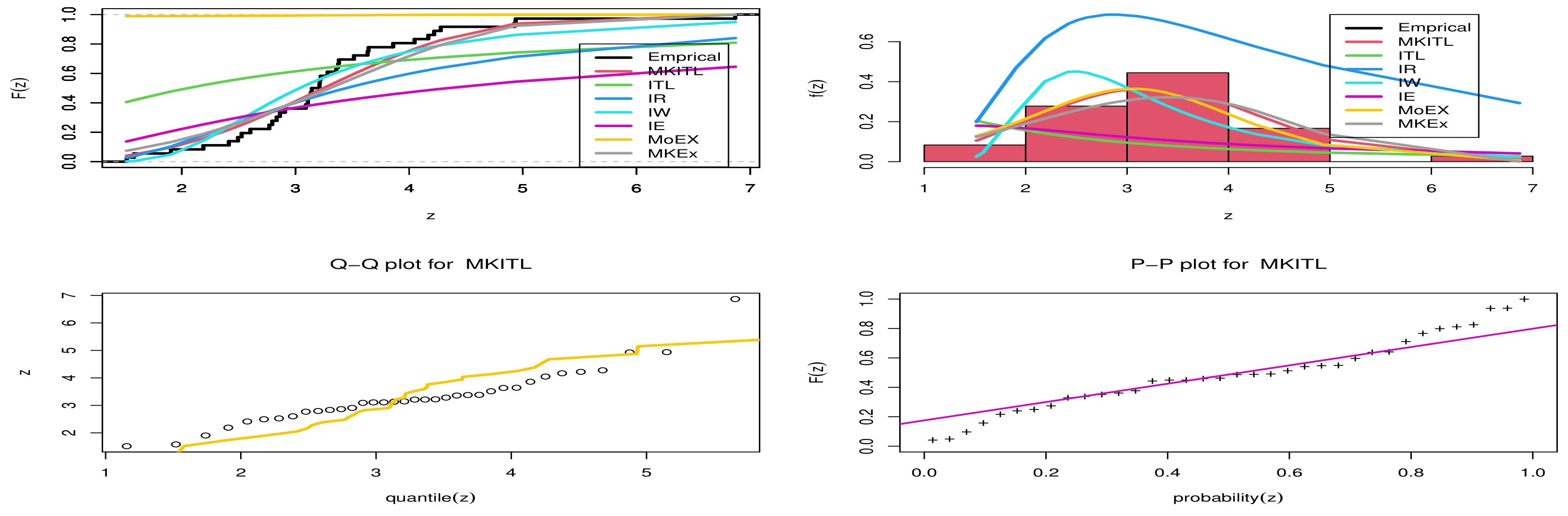
6.1. Application 1
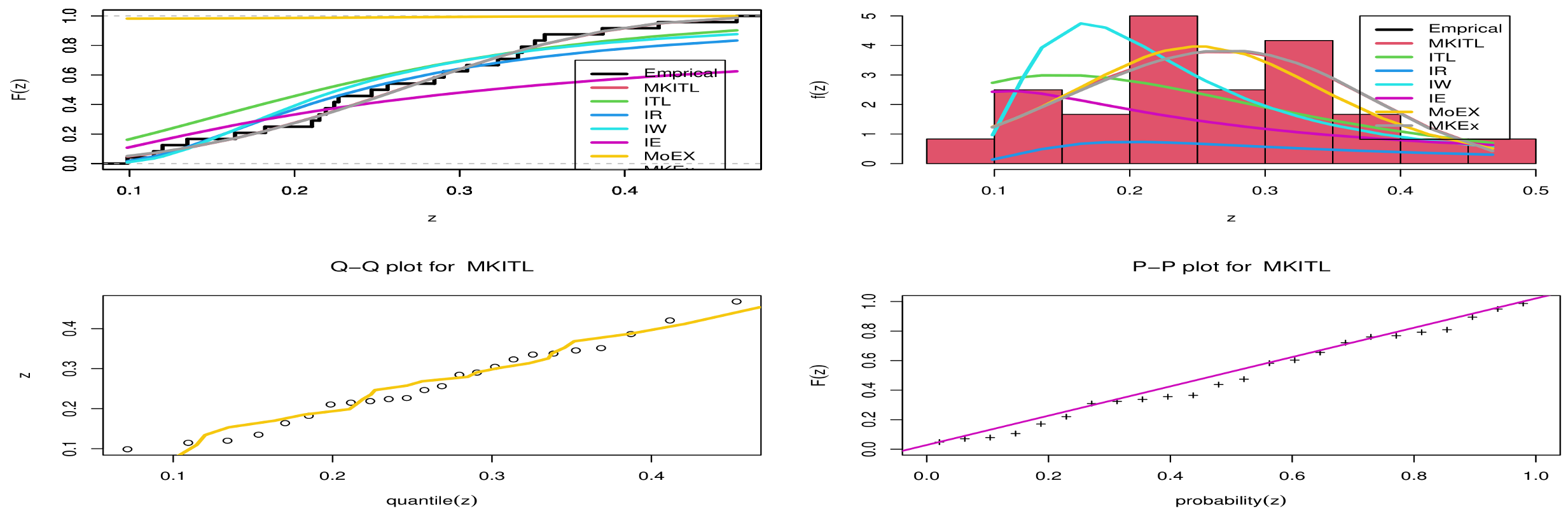
6.2. Application 2
6.3. Concluding Remarks on the Two Application
- Referring to data set one we can see that MKITL provides the highest P-value, and the lowest W*, A* and lowest KS distance.
- From Figure 3 , we can deduce that MKITL was the best model for fitting the first data set.
- Referring to data set two, we can see that MKITL provides the highest P-value, and the lowest A*, W* and KS distance.
- From Figure 4, we can deduce that MKITL was the best model for fitting the second data set.
- Referring to Table 4 we can see that IE, IR, ITL and MOEx distribution provides poor fitting for the first data set.
- Referring to Table 5 we can see that IE, MOEx distribution provides poor fitting for the second data set.
- We can conclude that from both applications that the MKITL distribution provides the best fitting among all its competitive distributions, which gives it superiority in fitting this kind of mortality rate for COVID-19 data.
7. Summary
Author Contributions
Funding
Conflicts of Interest
References
- Anake, T.A.; Oguntunde, P.E.; Odetunmibi, O.A. On a fractional beta- distribution. Int. J. Math. Comput. 2015, 26, 26–34. [Google Scholar]
- Abd AL-Fattah, A.M.; El-Helbawy, A.A.; Al-Dayian, G.R. Inverted Kumaraswamy Distribution: Properties and Estimation. Pak. J. Stat. 2017, 33, 37–61. [Google Scholar]
- Barco, K.V.P.; Mazucheli, J.; Janeiro, V. The inverse power Lindley distribution. Commun. Stat.-Simul. Comput. 2017, 46, 6308–6323. [Google Scholar] [CrossRef]
- Hassan, A.S.; Abd-Allah, M. On the inverse power Lomax distribution. Ann. Data Sci. 2019, 6, 259–278. [Google Scholar] [CrossRef]
- Muhammed, H.Z. On the inverted Topp Leone distribution. Int. J. Reliab. Appl. 2019, 20, 17–28. [Google Scholar]
- Chesneau, C.; Tomy, L.; Gillariose, J.; Jamal, F. The inverted modified Lindley distribution. J. Stat. Theory Pract. 2020, 14, 1–17. [Google Scholar] [CrossRef]
- Usman, R.M.; ul Haq, M.A. The Marshall-Olkin extended inverted Kumaraswamy distribution: Theory and applications. J. King Saud Univ.-Sci. 2020, 32, 356–365. [Google Scholar] [CrossRef]
- Eferhonore, E.E.; Thomas, J.; Zelibe, S.C. Theoretical Analysis of the Weibull Alpha Power Inverted Exponential Distribution: Properties and Applications. Gazi Univ. J. Sci. 2020, 33, 265–277. [Google Scholar]
- Kumar, S. Monitoring Novel Corona Virus (COVID-19) Infections in India by Cluster Analysis. Ann. Data Sci. 2020, 7, 417–425. [Google Scholar] [CrossRef]
- Khakharia, A.; Shah, V.; Jain, S.; Shah, J.; Tiwari, A.; Daphal, P.; Mehendale, N. Outbreak Prediction of COVID-19 for Dense and Populated Countries Using Machine Learning. Ann. Data Sci. 2020, 8, 1–19. [Google Scholar] [CrossRef]
- Wang, Y.z.J. A call for caution in extrapolating chest CT sensitivity for COVID-19 derived from hospital data to patients among general population. Quant. Imaging Med. Surg. 2020, 10, 798. [Google Scholar] [CrossRef]
- Lalmuanawma, S.; Hussain, J.; Chhakchhuak, L. Applications of machine learning and artificial intelligence for Covid-19 (SARS-CoV-2) pandemic: A review. Chaos Solitons Fractals 2020, 139, 110059. [Google Scholar] [CrossRef] [PubMed]
- Bullock, J.; Pham, K.H.; Lam, C.S.N.; Luengo-Oroz, M. Mapping the landscape of artificial intelligence applications against COVID-19. arXiv 2020, arXiv:2003.11336. [Google Scholar]
- Hassan, A.S.; Elgarhy, M.; Ragab, R. Statistical Properties and Estimation of Inverted Topp-Leone Distribution. J. Stat. Appl. Probab. 2020. forthcoming. [Google Scholar]
- Kumar, C.S.; Dharmaja, S.H.S. The exponentiated reduced Kies distribution: Properties and applications. Commun. Stat.-Theory Methods 2017, 46, 8778–8790. [Google Scholar] [CrossRef]
- Dey, S.; Nassar, M.; Kumar, D. Moments and estimation of reduced Kies distribution based on progressive type-II right censored order statistics. Hacet. J. Math. Stat. 2019, 48, 332–350. [Google Scholar] [CrossRef] [Green Version]
- Al-Babtain, A.A.; Shakhatreh, M.K.; Nassar, M.; Afify, A.Z. A New Modified Kies Family: Properties, Estimation Under Complete and type-II Censored Samples, and Engineering Applications. Mathematics 2020, 8, 1345. [Google Scholar] [CrossRef]
- Muhammed, H.Z.; Almetwally, E.M. Bayesian and Non-Bayesian Estimation for the Bivariate Inverse Weibull Distribution Under Progressive Type-II Censoring. Ann. Data Sci. 2020. [Google Scholar] [CrossRef]
- Almetwally, E.M.; Muhammed, H.Z. On a bivariate Fréchet distribution. J. Stat Appl Probab. 2020, 9, 1–21. [Google Scholar]
- El-Morshedy, M.; Alhussain, Z.A.; Atta, D.; Almetwally, E.M.; Eliwa, M.S. Bivariate Burr X generator of distributions: Properties and estimation methods with applications to complete and type-II censored samples. Mathematics. 2020, 8, 264. [Google Scholar] [CrossRef] [Green Version]
- Kim, J.M.; Ju, H.; Jung, Y. Copula Approach for Developing a Biomarker Panel for Prediction of Dengue Hemorrhagic Fever. Ann. Data Sci. 2020, 7, 697–712. [Google Scholar] [CrossRef]
- Almetwally, E.M.; Almongy, H.M.; Rastogi, M.K.; Ibrahim, M. Maximum Product Spacing Estimation of Weibull Distribution Under Adaptive Type-II Progressive Censoring Schemes. Ann. Data Sci. 2020, 7, 257–279. [Google Scholar] [CrossRef]
- Aslam, M.; Yousaf, R.; Ali, S. Bayesian Estimation of Transmuted Pareto Distribution for Complete and Censored Data. Ann. Data Sci. 2020, 7, 663–695. [Google Scholar] [CrossRef]
- Cheng, R.C.H.; Amin, N.A.K. Estimating parameters in continuous univariate distributions with a shifted origin. J. R. Stat. Soc. Ser. B (Methodol.) 1983, 45, 394–403. [Google Scholar] [CrossRef]
- Singh, R.K.; Singh, S.K.; Singh, U. Maximum product spacings method for the estimation of parameters of generalized inverted exponential distribution under Progressive Type II Censoring. J. Stat. Manag. Syst. 2016, 19, 219–245. [Google Scholar]
- Almetwally, E.M.; Almongy, H.M. Maximum product spacing and Bayesian method for parameter estimation for generalized power Weibull distribution under censoring scheme. J. Data Sci. 2019, 17, 407–444. [Google Scholar]
- Basu, S.; Singh, S.K.; Singh, U. Estimation of Inverse Lindley Distribution Using Product of Spacings Function for Hybrid Censored Data. Methodol. Comput. Appl. Probab. 2019, 21, 1377–1394. [Google Scholar] [CrossRef]
- Almetwally, E.M.; Almongy, H.M.; ElSherpieny, E.A. Adaptive type-II progressive censoring schemes based on maximum product spacing with application of generalized Rayleigh distribution. J. Data Sci. 2019, 17, 802–831. [Google Scholar]
- El-Sherpieny, E.S.A.; Almetwally, E.M.; Muhammed, H.Z. Progressive Type-II hybrid censored schemes based on maximum product spacing with application to Power Lomax distribution. Phys. A Stat. Mech. Its Appl. 2020, 553, 124251. [Google Scholar] [CrossRef]
- Alshenawy, R.; Al-Alwan, A.; Almetwally, E.M.; Afify, A.Z.; Almongy, H.M. Progressive Type-II Censoring Schemes of Extended Odd Weibull Exponential Distribution with Applications in Medicine and Engineering. Mathematics 2020, 8, 1679. [Google Scholar] [CrossRef]
- Alshenawy, R.; Sabry, M.A.; Almetwally, E.M.; Almongy, H.M. Product Spacing of Stress–Strength under Progressive Hybrid Censored for Exponentiated-Gumbel Distribution. Comput. Mater. Contin. 2021, 66, 2973–2995. [Google Scholar] [CrossRef]
- Luceno, A. Fitting the generalized Pareto distribution to data using maximum goodness of fit estimators. Comput. Stat. Data Anal. 2006, 51, 904–917. [Google Scholar] [CrossRef]
- Marshall, A.W.; Olkin, I. A new method for adding a parameter to a family of distributions with application to the exponential and Weibull families. Biometrika 1997, 84, 641–652. [Google Scholar] [CrossRef]
- Ahmad, A.; Ahmad, S.P.; Ahmed, A. Transmuted Inverse Rayleigh distribution: A generalization of the Inverse Rayleigh distribution. Math. Theory Model. 2014, 4, 90–98. [Google Scholar]


| MLE | LS | MPS | WLS | CVM | AD | |||||||||
|---|---|---|---|---|---|---|---|---|---|---|---|---|---|---|
| Mean | MSE | Mean | MSE | Mean | MSE | Mean | MSE | Mean | MSE | Mean | MSE | |||
| 0.6 | 25 | 0.5693 | 0.0167 | 0.6021 | 0.0180 | 0.5692 | 0.0131 | 0.6075 | 0.0164 | 0.6376 | 0.0223 | 0.6120 | 0.0152 | |
| 0.6114 | 0.0208 | 0.6191 | 0.0280 | 0.6113 | 0.0189 | 0.6194 | 0.0252 | 0.6331 | 0.0310 | 0.6196 | 0.0226 | |||
| 70 | 0.5839 | 0.0047 | 0.6024 | 0.0057 | 0.5839 | 0.0044 | 0.6055 | 0.0049 | 0.6145 | 0.0062 | 0.6058 | 0.0048 | ||
| 0.5990 | 0.0065 | 0.6046 | 0.0083 | 0.5990 | 0.0062 | 0.6046 | 0.0073 | 0.6091 | 0.0086 | 0.6050 | 0.0072 | |||
| 150 | 0.5892 | 0.0022 | 0.6008 | 0.0029 | 0.5891 | 0.0021 | 0.6028 | 0.0024 | 0.6064 | 0.0030 | 0.6023 | 0.0024 | ||
| 0.5988 | 0.0028 | 0.6022 | 0.0038 | 0.5987 | 0.0028 | 0.6027 | 0.0034 | 0.6043 | 0.0039 | 0.6026 | 0.0033 | |||
| 1.7 | 25 | 0.5777 | 0.0175 | 0.6178 | 0.0203 | 0.5779 | 0.0125 | 0.6227 | 0.0188 | 0.6542 | 0.0260 | 0.6248 | 0.0170 | |
| 1.7236 | 0.1568 | 1.7546 | 0.2115 | 1.7229 | 0.1391 | 1.7522 | 0.1883 | 1.7938 | 0.2350 | 1.7525 | 0.1714 | |||
| 70 | 0.5809 | 0.0051 | 0.6027 | 0.0062 | 0.5809 | 0.0048 | 0.6064 | 0.0056 | 0.6149 | 0.0068 | 0.6050 | 0.0052 | ||
| 1.7125 | 0.0550 | 1.7287 | 0.0781 | 1.7130 | 0.0514 | 1.7294 | 0.0678 | 1.7418 | 0.0813 | 1.7276 | 0.0646 | |||
| 150 | 0.5897 | 0.0022 | 0.6012 | 0.0027 | 0.5897 | 0.0022 | 0.6031 | 0.0024 | 0.6067 | 0.0028 | 0.6028 | 0.0023 | ||
| 1.7102 | 0.0226 | 1.7238 | 0.0304 | 1.7102 | 0.0215 | 1.7239 | 0.0265 | 1.7298 | 0.0311 | 1.7240 | 0.0264 | |||
| 3 | 25 | 0.5731 | 0.0180 | 0.6062 | 0.0196 | 0.5731 | 0.0135 | 0.6108 | 0.0180 | 0.6424 | 0.0245 | 0.6164 | 0.0168 | |
| 3.0467 | 0.4346 | 3.1018 | 0.6014 | 3.0466 | 0.3497 | 3.1171 | 0.6154 | 3.1728 | 0.6821 | 3.1198 | 0.5300 | |||
| 70 | 0.5811 | 0.0048 | 0.5982 | 0.0061 | 0.5811 | 0.0045 | 0.6018 | 0.0053 | 0.6102 | 0.0066 | 0.6018 | 0.0051 | ||
| 3.0047 | 0.1554 | 3.0384 | 0.2108 | 3.0047 | 0.1346 | 3.0384 | 0.1850 | 3.0616 | 0.2194 | 3.0396 | 0.1788 | |||
| 150 | 0.5924 | 0.0022 | 0.6016 | 0.0029 | 0.5923 | 0.0021 | 0.6045 | 0.0025 | 0.6072 | 0.0030 | 0.6040 | 0.0024 | ||
| 2.9988 | 0.0687 | 3.0243 | 0.0892 | 2.9989 | 0.0650 | 3.0249 | 0.0783 | 3.0348 | 0.0909 | 3.0238 | 0.0771 | |||
| MLE | LS | MPS | WLS | CVM | AD | |||||||||
|---|---|---|---|---|---|---|---|---|---|---|---|---|---|---|
| Mean | MSE | Mean | MSE | Mean | MSE | Mean | MSE | Mean | MSE | Mean | MSE | |||
| 0.6 | 25 | 1.5856 | 0.0862 | 1.6591 | 0.0890 | 1.5859 | 0.0791 | 1.6831 | 0.0833 | 1.7591 | 0.1119 | 1.7054 | 0.0786 | |
| 0.6037 | 0.0029 | 0.6047 | 0.0032 | 0.6036 | 0.0028 | 0.6059 | 0.0030 | 0.6094 | 0.0034 | 0.6072 | 0.0030 | |||
| 70 | 1.6483 | 0.0328 | 1.6898 | 0.0338 | 1.6482 | 0.0306 | 1.7088 | 0.0330 | 1.7220 | 0.0351 | 1.7100 | 0.0320 | ||
| 0.6004 | 0.0010 | 0.6012 | 0.0012 | 0.6003 | 0.0010 | 0.6017 | 0.0011 | 0.6028 | 0.0012 | 0.6019 | 0.0011 | |||
| 150 | 1.6706 | 0.0146 | 1.7023 | 0.0182 | 1.6706 | 0.0144 | 1.7098 | 0.0154 | 1.7185 | 0.0189 | 1.7101 | 0.0158 | ||
| 0.5998 | 0.0005 | 0.6005 | 0.0006 | 0.5998 | 0.0005 | 0.6007 | 0.0005 | 0.6012 | 0.0006 | 0.6008 | 0.0005 | |||
| 1.7 | 25 | 1.6116 | 0.1145 | 1.7011 | 0.1276 | 1.6117 | 0.0896 | 1.7188 | 0.1152 | 1.8055 | 0.1582 | 1.7370 | 0.1032 | |
| 1.7086 | 0.0237 | 1.7105 | 0.0252 | 1.7086 | 0.0227 | 1.7139 | 0.0240 | 1.7238 | 0.0266 | 1.7173 | 0.0239 | |||
| 70 | 1.6371 | 0.0307 | 1.6867 | 0.0385 | 1.6373 | 0.0308 | 1.7001 | 0.0337 | 1.7221 | 0.0407 | 1.7017 | 0.0324 | ||
| 1.7028 | 0.0075 | 1.7042 | 0.0086 | 1.7027 | 0.0074 | 1.7058 | 0.0080 | 1.7089 | 0.0088 | 1.7067 | 0.0080 | |||
| 150 | 1.6671 | 0.0140 | 1.7032 | 0.0195 | 1.6670 | 0.0140 | 1.7092 | 0.0161 | 1.7198 | 0.0204 | 1.7083 | 0.0156 | ||
| 1.7003 | 0.0035 | 1.7019 | 0.0040 | 1.7002 | 0.0034 | 1.7026 | 0.0038 | 1.7040 | 0.0041 | 1.7028 | 0.0037 | |||
| 3 | 25 | 1.6110 | 0.1158 | 1.7090 | 0.1431 | 1.6113 | 0.0897 | 1.7256 | 0.1267 | 1.8146 | 0.1798 | 1.7391 | 0.1109 | |
| 2.9987 | 0.0649 | 3.0010 | 0.0731 | 2.9985 | 0.0623 | 3.0065 | 0.0690 | 3.0247 | 0.0766 | 3.0119 | 0.0677 | |||
| 70 | 1.6407 | 0.0306 | 1.7040 | 0.0445 | 1.6407 | 0.0301 | 1.7128 | 0.0364 | 1.7400 | 0.0485 | 1.7116 | 0.0338 | ||
| 3.0027 | 0.0264 | 3.0074 | 0.0300 | 3.0025 | 0.0259 | 3.0099 | 0.0282 | 3.0156 | 0.0306 | 3.0104 | 0.0280 | |||
| 150 | 1.6627 | 0.0137 | 1.6982 | 0.0187 | 1.6628 | 0.0142 | 1.7040 | 0.0159 | 1.7147 | 0.0194 | 1.7033 | 0.0152 | ||
| 3.0005 | 0.0118 | 3.0028 | 0.0130 | 3.0003 | 0.0117 | 3.0040 | 0.0122 | 3.0066 | 0.0131 | 3.0042 | 0.0122 | |||
| MLE | LS | MPS | WLS | CVM | AD | |||||||||
|---|---|---|---|---|---|---|---|---|---|---|---|---|---|---|
| Mean | MSE | Mean | MSE | Mean | MSE | Mean | MSE | Mean | MSE | Mean | MSE | |||
| 0.6 | 25 | 2.8337 | 0.1408 | 2.8969 | 0.1058 | 2.8339 | 0.1606 | 2.9309 | 0.0985 | 2.9607 | 0.0714 | 2.9618 | 0.0585 | |
| 0.5988 | 0.0009 | 0.5991 | 0.0011 | 0.5988 | 0.0009 | 0.5999 | 0.0010 | 0.6010 | 0.0011 | 0.6005 | 0.0010 | |||
| 70 | 2.9155 | 0.0496 | 2.9782 | 0.0295 | 2.9156 | 0.0506 | 2.9962 | 0.0259 | 3.0149 | 0.0344 | 2.9865 | 0.0424 | ||
| 0.5982 | 0.0003 | 0.5991 | 0.0004 | 0.5982 | 0.0003 | 0.5994 | 0.0003 | 0.5999 | 0.0004 | 0.5996 | 0.0003 | |||
| 150 | 2.9443 | 0.0275 | 2.9853 | 0.0082 | 2.9440 | 0.0238 | 3.0012 | 0.0129 | 2.9954 | 0.0083 | 2.9949 | 0.0090 | ||
| 0.5994 | 0.0001 | 0.6001 | 0.0002 | 0.5994 | 0.0001 | 0.6002 | 0.0002 | 0.6004 | 0.0002 | 0.6003 | 0.0002 | |||
| 1.7 | 25 | 2.8113 | 0.3529 | 2.9196 | 0.2694 | 2.8113 | 0.2987 | 2.9733 | 0.2791 | 3.0759 | 0.2844 | 3.0107 | 0.2637 | |
| 1.7034 | 0.0080 | 1.7038 | 0.0085 | 1.7034 | 0.0077 | 1.7057 | 0.0081 | 1.7113 | 0.0088 | 1.7085 | 0.0080 | |||
| 70 | 2.8962 | 0.0967 | 2.9926 | 0.1139 | 2.8966 | 0.0970 | 3.0082 | 0.0987 | 3.0529 | 0.1203 | 3.0167 | 0.1010 | ||
| 1.7005 | 0.0027 | 1.7022 | 0.0030 | 1.7005 | 0.0027 | 1.7028 | 0.0029 | 1.7048 | 0.0031 | 1.7032 | 0.0028 | |||
| 150 | 2.9470 | 0.0445 | 2.9955 | 0.0457 | 2.9468 | 0.0435 | 3.0217 | 0.0452 | 3.0213 | 0.0454 | 3.0175 | 0.0429 | ||
| 1.6974 | 0.0013 | 1.6970 | 0.0014 | 1.6974 | 0.0013 | 1.6981 | 0.0013 | 1.6981 | 0.0014 | 1.6982 | 0.0013 | |||
| 3 | 25 | 2.8351 | 0.3245 | 2.9918 | 0.3290 | 2.8347 | 0.2596 | 3.0273 | 0.3148 | 3.1730 | 0.4019 | 3.0626 | 0.2887 | |
| 2.9931 | 0.0229 | 2.9967 | 0.0251 | 2.9933 | 0.0224 | 2.9996 | 0.0239 | 3.0099 | 0.0258 | 3.0031 | 0.0236 | |||
| 70 | 2.9073 | 0.0946 | 3.0050 | 0.1201 | 2.9072 | 0.0896 | 3.0279 | 0.1075 | 3.0684 | 0.1303 | 3.0275 | 0.1001 | ||
| 3.0017 | 0.0079 | 3.0027 | 0.0086 | 3.0018 | 0.0078 | 3.0045 | 0.0081 | 3.0074 | 0.0088 | 3.0051 | 0.0080 | |||
| 150 | 2.9351 | 0.0390 | 2.9925 | 0.0530 | 2.9349 | 0.0405 | 3.0076 | 0.0447 | 3.0218 | 0.0546 | 3.0055 | 0.0435 | ||
| 2.9967 | 0.0040 | 2.9981 | 0.0044 | 2.9968 | 0.0040 | 2.9991 | 0.0041 | 3.0003 | 0.0044 | 2.9990 | 0.0041 | |||
| KS | p-Value | W * | A * | ||||
|---|---|---|---|---|---|---|---|
| MKITL | MLE | 3.3555 | 0.7286 | 0.1454 | 0.4323 | 0.1087 | 0.6473 |
| SE | 0.4046 | 0.0275 | |||||
| MKEx | MLE | 2.2855 | 0.1864 | 0.1695 | 0.2523 | 0.2299 | 1.3306 |
| SE | 0.2705 | 0.0103 | |||||
| IW | MLE | 3.1691 | 23.4053 | 0.1737 | 0.2274 | 0.2548 | 1.5284 |
| SE | 0.3656 | 8.1037 | |||||
| IR | MLE | 8.2339 | 0.2790 | 0.0074 | 0.1770 | 1.0691 | |
| SE | 1.3723 | ||||||
| IE | MLE | 3.0078 | 0.4284 | 0.0000 | 0.1289 | 0.7751 | |
| SE | 0.5013 | ||||||
| ITL | MLE | 1.1523 | 0.4390 | 0.0000 | 0.1505 | 0.8600 | |
| SE | 0.1920 | ||||||
| MOEx | MLE | 83.0836 | 1.4411 | 0.9890 | 0.0000 | 0.3894 | 2.2258 |
| SE | 39.1521 | 0.1530 |
| KS | p-Value | W* | A* | ||||
|---|---|---|---|---|---|---|---|
| MKITL | MLE | 1.3599 | 12.7931 | 0.0936 | 0.9715 | 0.0244 | 0.1762 |
| SE | 0.2319 | 1.4051 | |||||
| MKEX | MLE | 2.1755 | 2.3241 | 0.0956 | 0.9658 | 0.0254 | 0.1831 |
| SE | 0.3598 | 0.1636 | |||||
| ITL | MLE | 21.7398 | 0.2371 | 0.1136 | 0.0403 | 0.2776 | |
| SE | 4.4376 | ||||||
| IR | MLE | 0.0399 | 0.1666 | 0.4685 | 0.1541 | 0.9476 | |
| SE | 0.0081 | ||||||
| IW | MLE | 2.3035 | 0.0229 | 0.1869 | 0.3292 | 0.1698 | 1.0330 |
| SE | 0.3350 | 0.0149 | |||||
| IE | MLE | 0.2200 | 0.3752 | 0.0015 | 0.1052 | 0.6731 | |
| SE | 0.0449 | ||||||
| MOEX | MLE | 50.8938 | 15.5659 | 0.9817 | 0.0000 | 0.1196 | 0.7700 |
| SE | 36.2538 | 2.5549 |
Publisher’s Note: MDPI stays neutral with regard to jurisdictional claims in published maps and institutional affiliations. |
© 2021 by the authors. Licensee MDPI, Basel, Switzerland. This article is an open access article distributed under the terms and conditions of the Creative Commons Attribution (CC BY) license (http://creativecommons.org/licenses/by/4.0/).
Share and Cite
Almetwally, E.M.; Alharbi, R.; Alnagar, D.; Hafez, E.H. A New Inverted Topp-Leone Distribution: Applications to the COVID-19 Mortality Rate in Two Different Countries. Axioms 2021, 10, 25. https://0-doi-org.brum.beds.ac.uk/10.3390/axioms10010025
Almetwally EM, Alharbi R, Alnagar D, Hafez EH. A New Inverted Topp-Leone Distribution: Applications to the COVID-19 Mortality Rate in Two Different Countries. Axioms. 2021; 10(1):25. https://0-doi-org.brum.beds.ac.uk/10.3390/axioms10010025
Chicago/Turabian StyleAlmetwally, Ehab M., Randa Alharbi, Dalia Alnagar, and Eslam Hossam Hafez. 2021. "A New Inverted Topp-Leone Distribution: Applications to the COVID-19 Mortality Rate in Two Different Countries" Axioms 10, no. 1: 25. https://0-doi-org.brum.beds.ac.uk/10.3390/axioms10010025