We will illustrate Theorem 1 with two examples. We will use these two examples to construct models in economics and ecology.
4.1. Examples
Example 1: Let us choose
,
, so that
Let us define the maps
by
Let us denote
and
. Let us endow
with the absolute value metrics
. Let us consider the sets
,
. Let us define the multivalued maps
and
by
and
We will check that F and G satisfy Theorem 1.
It is easy to see that for any the sets and are non empty and closed subsets of X or Y, respectively.
From
and
we get that
and
. Then
for any
and any
.
From and it follows that and for .
There are four cases:
(I) and ; (II) and ; (III) and ; (IV) and .
We will need the inequalities:
and
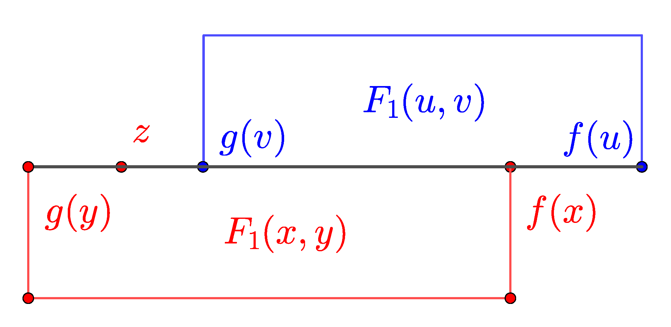
Case (I). We will illustrate this case with a figure for easier reading (
Figure 1). The other three cases are similar.
Case (II). In this case
and we get
Case (III). In this case
and we get
Case (IV). This case is very similar to case I) and we get
Therefore by combining the four Cases (I) to (IV) we get
By similar calculations we can get that
Thus there holds the inequality
A particular case can be obtained if
,
,
,
,
and
. We get
,
,
,
and
Example 2. Let us consider the space
. Let us choose
,
for
, so that
and
Let us define the maps
for
by
where
and
.
Let us denote
and
for
. Let us endow
with the metrics
,
. Let us consider the sets
,
for
and let
,
. Let us define the multivalued maps
and
by
and
We will check that the pair satisfies Theorem 1.
Let us choose
and
. By definition
It is easy to see that
, where
be the rectangular with vertices
,
,
,
and
be the rectangular with vertices
,
,
,
and
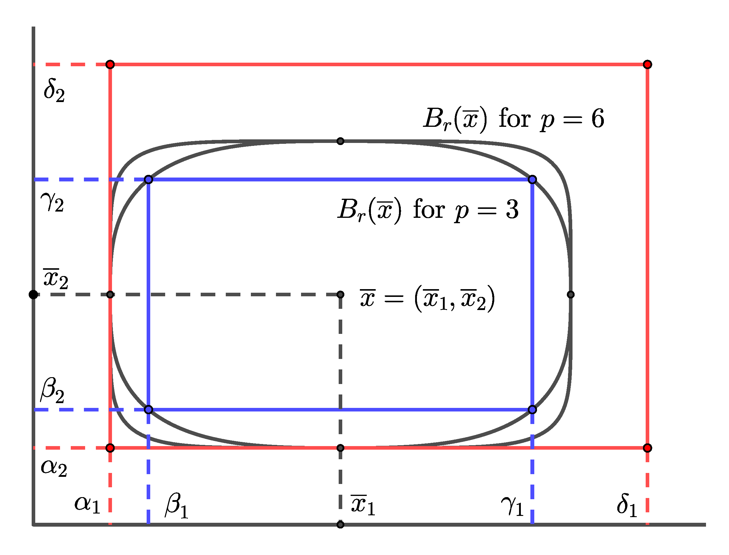
(
Figure 2) is an ellipse for
.
Indeed, let
. Then
. Thereafter it holds for
and consequently we can write the inequalities
From it follows that and from it follows that and therefore holds for any and .
We observe that there hold and . Therefore we will need to calculate and .
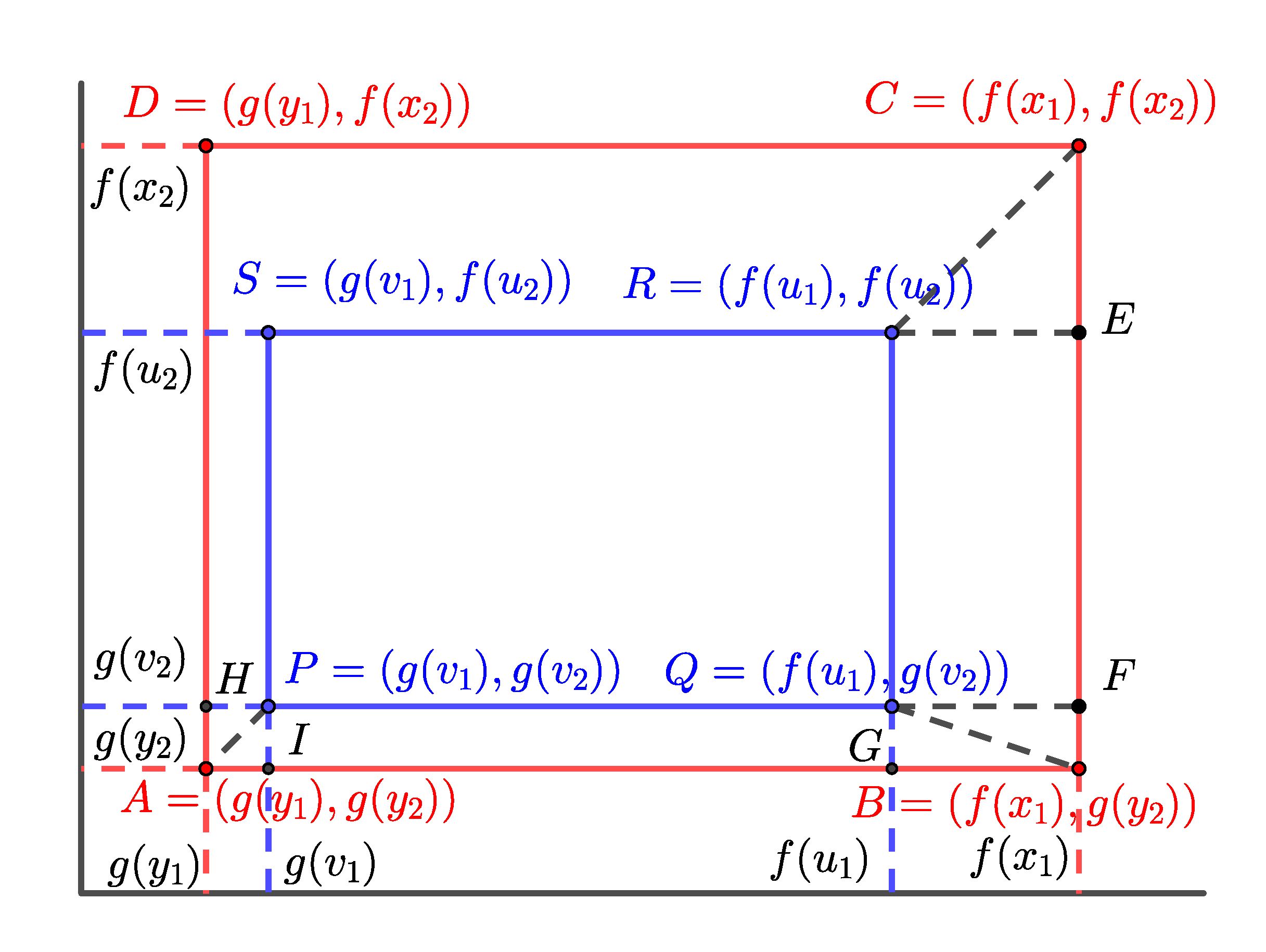
The set is a rectangular with vertexes , , and . There are several possible cases: , or and or with all the possible combinations of .
Let us first consider the case:
and
. It is easy to observe that
(
Figure 3), where
We will need the inequalities:
where
and
and
For the estimation of
and
let us denote (
Figure 3)
By similar observation we can prove that
Consequently
, where
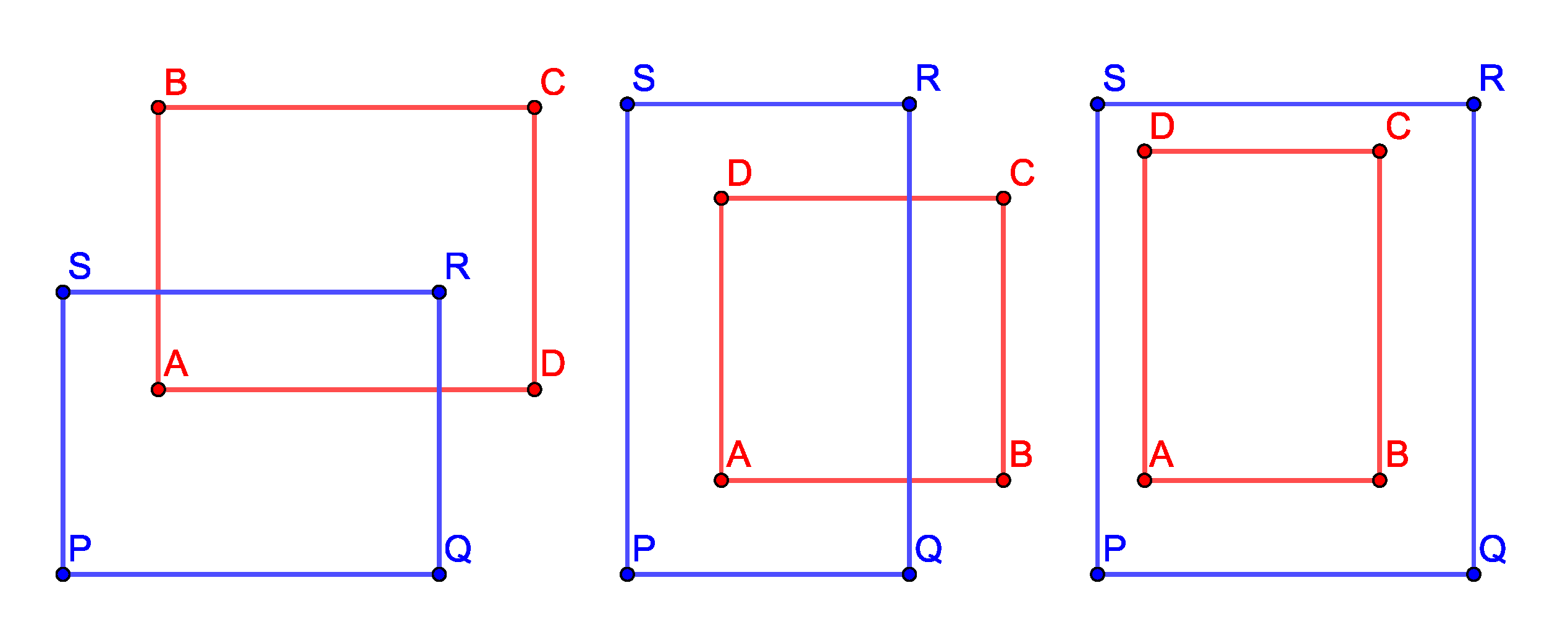
Let us denote the two rectangles
and
by
and
, respectively. We have just investigated the case
. All the other cases are variants of
Figure 4 and we can get that
By similar calculations for the multivalued map
G we get
where
and thus
4.2. Examples for the Existence of an Equilibrium in Oligopoly (Duopoly) Markets
The theory of oligopoly (duopoly) markets was initiated in [
21]. Following [
22,
23] we present the main features of an oligopoly model in economics. The oligopoly is a market structure in the presence of imperfect competition in which a limited number of large companies control the production and sale of a predominant part of the product in a particular sector of the economy. It is believed that oligopolies are the result of the trend in the economy towards concentration of capital and labor. The oligopoly is characterized by product differentiation; high barriers preventing the emergence of new “players”; limited access to information; non-price competition through advertising and other marketing activities, as well as price control. In the oligopolistic structure, large companies determine the behavior of competitors and take it into account when developing their strategy, which can be rivalry, even “trade wars” in terms of production volume, sales, and prices; the strategic interaction results in agreements (through secret or open collusion or without collusion) in order to guarantee stability and ensure high profits. They contribute to raising economic and organizational barriers, making it difficult for new “players” to emerge. This is the nature of the large initial capital costs for entering the business and achieving minimum effective production and sales capacity in view of economies of scale and resilience against competitors, the development of own research and development for product innovation, industrial and trade secrets. Oligopolistic market structures arise and are imposed by three key points (1) the concentration of assets; (2) inter-firm agreements; and (3) fencing off activities in order to gain market power, restrict competition, and generate large profits.
The distinctive feature of the oligopoly is that in determining individual supply and market price, companies are interdependent. The change in the market behavior of each of them can lead to a change in market conditions and possibly cause a change in the behavior of other companies.
The equilibrium quantity and price in the oligopoly will depend on the number of firms on the market, the information available, the strategy chosen by competitors and whether the firms in the market act independently of each other or in concert. The latter factor is the basis for two types of oligopolistic equilibrium-coherent and inconsistent, which differ significantly in end results and economic efficiency.
The classic model of uncoordinated oligopolistic behavior is the Cournot duopoly model, which considers the problem of the interdependence of firms in the market. The duopoly is a market structure in which two companies, protected from the emergence of other sellers, act as the only producers of standardized products that have no close substitutes, in which there are only two sellers of a particular product that are not interconnected by monopolistic agreement for prices market for selling products and quotas. The participants in the model try to maximize their payoff functions and , respectively, where be the inverse of the demand function and and be the cost functions of the two players. By maximizing its payoff functions, the players get their response functions and , respectively.
The company equilibrium would become market if the supply of one company is equal to the supply of the other company, so that none of the companies is motivated to change their positions condition for market equilibrium. This condition is present if each of the companies produces one third of the total market supply under conditions of perfect competition and both companies sell at a specific market price, which is one third of the market price. Taking into account the strategic considerations of the companies, their behavior will depend on the decisions of their competitors.
Cournot’s theory is based on competition and the fact that buyers announce prices and sellers adjust their products to those prices. Each company evaluates the product search function and then sets the quantity that will be sold, assuming that the competitor’s output remains constant.
Deeper research on the oligopoly market can be found in [
22,
23,
24,
25].
Cournot’s classical model deals with a maximization of the payoff functions of each of the players. A different approach is presented in [
18], where attention is paid to the response functions of the players. The benefits of this approach are commented on in [
18]. We will just say that as far as the players do not have a perfect knowledge of the market they react in some sense by not maximizing their payoff function, but rather by choosing a strategy based on their production and their rival’s production levels. The solution of the maximization of the payoff function is actually the coupled fixed points
, such that
and
.
Focusing on response functions allows us to put Cournot and Bertand’s models together. Indeed let the first company reaction be and the second one , where and . Here x and y denote the output quantity and are the prices set by players. In this, companies can compete in terms of both price and quantity.
A disadvantage of the presented model is that players do not choose a fixed production of a fixed price. Actually, the response of each player is any quality from a set of possible productions or a price from possible prices. Therefore we will consider the response functions and be multivalued maps and a market equilibrium will be the pair , such that and .
Now we can restate Theorem 1 in terms of oligopoly.
Theorem 2. Let us assume that two companies are offering products that are perfect substitutes. The first one can produce qualities from the set X and the second firm can produce qualities from the set Y, where X and Y be nonempty subsets of a partially ordered complete metric space and . Consider and to be the response function of players one and two, respectively. Let F and G satisfy all the conditions in Theorem 1.
Then there exists at least one market equilibrium point , which is a coupled fixed point for the ordered pair of response functions .
Example 3: Let us consider in Example 1 two firms, producing one commodity, which is a perfect substitute. Let us put
,
,
,
and
in Example 1. We may consider the interval
as the set of the total production. Let the first firm be a smaller one and its production set is
and the second one be a larger firm with a production set
. Let
and
. Then for any initial start
in the market the first firm chooses a production from the set
and the second firm from the set
and
where
. From
it follows that the pair of response functions satisfies Theorem 2 and consequently there exists an equilibrium pair of productions
, such that
and
.
Example 4. Let us consider a model of a duopoly with two players, producing one good, which is a complete substitute, and let they compete on qualities and prices simultaneously. Let us choose in Example 2, , , , , , , , , , , , , . Let us consider the sets , for and let , and the multivalued maps and from Example 2, which are the response functions of the two players, respectively, where the first coordinates are the response on the qualities and the second coordinate is the response on the price. Let us endow with the metrics , from Example 2.
From the inequality it follows that we can apply Theorem 2. Consequently there exists an equilibrium pair of productions and prices , such that and . The actual values of , , and are smaller.


 ,
, 


